On approximating copulas by finite mixtures

Abstract.

Copulas are now frequently used to construct or estimate multivariate distributions because of their ability to take into account the multivariate dependence of the different variables while separately specifying marginal distributions. Copula based multivariate models can often also be more parsimonious than fitting a flexible multivariate model, such as a mixture of normals model, directly to the data.

However, to be effective, it is imperative that the family of copula models considered is sufficiently flexible. Although finite mixtures of copulas have been used to construct flexible families of copulas, their approximation properties are not well understood and we show that natural candidates such as mixtures of elliptical copulas and mixtures of Archimedean copulas cannot approximate a general copula arbitrarily well. Our article develops fundamental tools for approximating a general copula arbitrarily well by a copulas based on finite mixtures. We show the asymptotic properties as well as illustrate the advantages of our methodology empirically on a financial data set and on some artificial data.

Keywords: Archimedean copula; Elliptical copula; Finite mixtures; Mixtures of copulas; Nonparametric estimation.

1. Introduction

The purpose of this paper is to establish a new methodology for the non-parametric estimation of copulas through the use of sieves based on finite mixture models. As good approximation properties of finite mixtures are an indispensable prerequisite for their use in non-parametric estimation, the paper mainly focuses on establishing a mathematical theory for proving approximation properties of those mixtures. Those properties are not only of mathematical interest in their own right, but they also bring the whole machinery of mixture modeling to bear down on the problem of estimating copulas non-parametrically or to a lesser extent modeling them in an optimal way by combining flexibility with parsimony.

Our article provides some foundational tools for using finite mixture models to non-parametrically estimate a target copula function $C$, having density $c$, by asking under what conditions can we find a positive integer $R$, cumulative distribution functions $G_{1},\dots,G_{R}$, and positive probabilities $\pi_{1},\dots,\pi_{R}$ satisfying $\pi_{1}+\cdots+\pi_{R}=1$ to approximate $C$ by $G:=\pi_{1}G_{1}+\cdots+\pi_{R}G_{R}$ for a given precision. Or, alternatively, under what conditions can we find probability density functions $g_{1},\dots,g_{R}$, to approximate the density $c$ by $g:=\pi_{1}g_{1}+\cdots+\pi_{R}g_{R}$ for a given precision. Our main result uses this framework to propose a copula family based on a finite mixture that can approximate any copula arbitrarily well. The summary at the end of the paper further discusses the statistical application of these results.

Our article also shows that neither mixtures of Archimedean copulas nor mixtures of elliptical copulas can in general approximate a copula density arbitrarily well. Even though they are natural candidate families that have been extensively used to approximate an arbitrary copula, the literature contains no mathematical results on how good their approximation properties are.

The methodology introduced in this paper is not only of interest when it comes to approximating copulas, but it is also useful for approximating arbitrary distributions. Indeed, using a copula-based approach for approximating multivariate distributions involves approximating each of the marginals separately while also approximating the underlying implied joint distribution. Such an approach for approximating multivariate distributions is attractive for two reasons. First, we can directly control the properties of the approximating marginal distributions rather than just deducing their properties from the approximation of the joint. For example, consider approximating a high dimensional multivariate model by a flexible factor based model such as a mixture of factor analyzers; see, for example, Chapter 8 of McLachlan and Peel, (2000). It is then difficult to ensure that the implied marginal distributions will be consistent with an approach that approximates the marginal distributions directly. A second attractive property of copulas is that a copula based multivariate approximation can often be much more parsimonious than approximating the multivariate distribution directly. For example, consider a bivariate distribution with independent marginals each of which is a 6 component mixture of normals. Then approximating this distribution by a bivariate mixture of normals will require a 36 component mixture, while a copula based approach will fit a 6 component mixture to each of the marginals and then a standard normal for the underlying Gaussian copula. Section 2.4 illustrates the same issue on a more complex example. However, it is imperative when using a copula based approach to approximate multivariate distributions that the family of approximating copulas is sufficiently flexible. The reason is that the copula is formed by transforming each of the marginals to a uniform distribution, which can potentially make the underlying distribution of the copula quite complex. Tran et al., (2014) show empirically that this can happen, for example, when the original multivariate distribution is heavy tailed or multimodal.

We now briefly review the literature on nonparametric estimation of copulas. The foundation of non-parametric estimation is based on estimating the copula cumulative distribution function (CDF) using empirical copulas and studying the asymptotic weak convergence properties of the empirical copula process. See, for example, Fermanian et al., (2004) and Segers, (2012). Among density estimators, Bernstein copulas constitute a prominent example; see Sancetta and Satchell, (2004) and Sancetta, (2007), or Burda and Prokhorov, (2014) for a Bayesian approach. Currently, Bernstein copulas do not scale well with the dimension of the multivariate distribution and applications have been restricted to small dimensions as the number of parameters increases exponentially with dimension. Some other approaches are based on kernels (Omelka et al.,, 2009) and wavelets (Genest et al.,, 2009). There are very few papers that explicitly address the question of estimating copulas non-parametrically through the use of mixtures. Wu et al., (2014) and Wu et al., (2015) present a Bayesian non-parametric approach. Wu et al., (2014) take Gaussian copulas as the mixture components. Wu et al., (2015) take multivariate skew normal copulas as the mixture components. However, neither paper presents approximation results.

Our approach has several advantages compared to competing approaches in the literature on dense subfamilies for approximating copulas; see, for example, Chapter 4 in Durante and Sempi, (2015) for a excellent review. First, because our approach is mixture based, we can use the vast statistical and computational literature on estimating mixtures. Furthermore, compared to some more tractable approximating dense families like Bernstein copulas, our approach is more parsimonious in certain cases because the number of “effective parameters” that require estimation grows quadratically in the number of dimensions instead of exponentially. Finally, our approach is attractive because it automatically yields an easily computable valid copula for the approximation.

The rest of the paper is organized as follows. Section 2 presents our fundamental approximation results and constructs a family of mixture models that can approximate any copula arbitrarily well. Section 2.4 uses a simple example to illustrate our approximation approach. Section 3 introduces a concentration inequality useful for illustrating the asymptotic properties of the mixture family. Sections 4 and 5 respectively characterize Archimedean and elliptical copulas and discuss their approximation properties. Section 6 applies our approximation approach to a financial data set that was previously analyzed in the literature. We show that our approach provides a better fit and is more parsimonious than that obtained by a mixture of Gaussian copulas. There are two technical appendices. Appendix A contains all the proofs. Appendix B shows how to sample from the specific copula we use for the illustration in Section 2.4. Section 7 concludes by discussing future theoretical and computational work based on our results.

2. Approximation properties of some mixtures of general distributions on the unit hypercube

We first consider approximating some distributions on the unit interval $(0,1)$, and then consider the case of classes of copulas on $(0,1)^{M}$. The reason for starting with the unit interval is that we can introduce our methodology and some main ideas in a simpler setting before focusing on our main objective, which is the approximation of copulas and copula densities.

There is an extensive literature on approximating arbitrary distributions by finite mixtures. See Zeevi and Meir, (1997), Dalal and Hall, (1983) or Lijoi, (2003). We will use the elements of the theory of approximation by universal series (see Bacharoglou, (2010) and Koumandos et al., (2010)) to obtain our approximations.

We begin by stating an adaptation of a theorem from Bacharoglou, (2010) that is essential for deriving our main results. The theorem is based on the theory of Universal series in $\bigcap_{p>1}\ell^{p}$ and yields approximations in $\|\cdot\|$ over certain subsets of $\mathbb{R}^{M}$ for bounded continuous functions or functions with bounded support. Here $\ell^{p}$ stands for the traditional $p$-power summable sequence spaces and $\|\cdot\|$ means either the $L_{1}$ or the $L_{\infty}$ norm, or their sum. That norm is used in the statement of Theorem 1. Otherwise, if the result concerns a specific norm, then we will denote it by either$\|\cdot\|_{1}$ or $\|\cdot\|_{\infty}$ if necessary. Also, let $\mathbb{N}$ be the set of positive integers and let $\mathbb{Q}$ be the set of rational numbers.

Theorem 1.

Let

$$\mathcal{A}^{+}=\left\{\alpha=(\alpha_{n})_{n\in\mathbb{N}},\alpha_{n}>0,\,\,\,\text{for every}\leavevmode\nobreak\ n,\alpha\in\bigcap_{p>1}\ell^{p}\right\},$$

and let the sequence $(\phi_{n})_{n}$ be formed by enumerating $\phi_{\frac{1}{k}}(\boldsymbol{x}-\boldsymbol{\mu})$, where $k\in\mathbb{N}$, $\boldsymbol{\mu}\in\mathbb{Q}^{M}$ (some enumeration of it) and $\phi_{s}(\boldsymbol{x}-\boldsymbol{\mu})$ is the density of a multivariate normal distribution with mean vector $\boldsymbol{\mu}$ and covariance matrix $s\boldsymbol{I}_{M}$. Let $f$ be some density that has either compact support on $\mathbb{R}^{M}$ or that is bounded and continuous.

Then, there exists an $\alpha\in\mathcal{A^{+}}$ and a sequence $(R_{n})_{n}$ of integers such that for all $\varepsilon>0$, there exists an $n(\varepsilon)$ such that for all integers $n>n(\varepsilon)$, the following holds

$$\left\|f-\frac{1}{\sum_{j=1}^{R_{n}}\alpha_{j}}\sum_{j=1}^{R_{n}}\alpha_{j}\phi_{j}\right\|<\varepsilon.$$

2.1. Approximation on the unit interval

Let $F$ be the cumulative distribution function of an absolutely continuous random variable $X$. If one applies the transformation $F$ to $X$, then it immediately follows by a simple calculation that the transformed random variable $F(X)$ is uniform on $(0,1)$,

$$\Pr[F(X)\leqslant t] =\Pr[X\leqslant F^{-1}(t)]$$

$$=F\circ F^{-1}(t)=t.$$

If one applies a different transformation (say using a different distribution function $H$), then we obtain that the distribution of the transformed random variable $H(X)$ is

$$\Pr[H(X)\leqslant t] = F\circ H^{-1}(t).$$

If $H$ is the distribution of an absolutely continuous random variable, then $H(X)$ is an absolutely continuous random variable on $(0,1)$, but is not uniform in general. Theorem 2 exploits such simple constructions by using them as building blocks for finite mixture distributions. In particular, the theorem exploits distributions of the form $F\circ H^{-1}(t)$ in order to approximate densities (or distributions) on $(0,1)$.

Theorem 2.

Let $g$ be an unknown continuous density function with compact support in $(0,1)$. Let $h$ be some arbitrary bounded and absolutely continuous density function with its support being the whole real line and let $H$ be its corresponding CDF. Let $\phi_{\mu,\sigma}$ be a normal density with mean $\mu$ and standard deviation $\sigma$. Then, for every $\varepsilon>0$, there exist an $R\in\mathbb{N}$, $(\pi_{1},\ldots,\pi_{R})\in\Delta_{R}$ (the $R$-simplex), $\mu_{1},\ldots,\mu_{R}\in\mathbb{R}$ and $\sigma_{1},\ldots,\sigma_{R}\in(0,\infty)$ such that

$$\left\|g-\sum_{r=1}^{R}\pi_{r}\frac{\phi_{\mu_{r},\sigma_{r}}\circ H^{-1}}{h\circ H^{-1}}\right\|<\varepsilon,$$

where $\|\cdot\|$ is either the $L_{1}$ or $L_{\infty}$ norm.

Even though the theorem is stated for the approximation of a density $g$, it can be used with no additional difficulty to approximate an arbitrary continuous cumulative distribution, say $G$. This is a particularly important point, as the results of this paper can be used to approximate either the distribution of a random variable, or, with some extra assumptions, the density of that random variable. The next section extends theorem 2 to the multivariate setting and shows how to approximate a copula and its density.

2.2. Approximation of copulas

Theorem 3 applies the same reasoning as the approximation result on unit intervals to get an approximation result for copulas in terms of distributions on $(0,1)^{M}$. Let $H$ be the CDF of an $M\times 1$ random vector, with marginal distribution functions $H_{1},\dots,H_{M}$ and define $\mathfrak{F}_{H}:\mathbb{R}^{M}\rightarrow(0,1)^{M}$ as $\mathfrak{F}_{H}(\boldsymbol{x}):=\left(H_{1}(x_{1}),\dots,H_{M}(x_{M})\right)$ We similarly define $\mathfrak{F}_{H}^{-1}:(0,1)^{M}\rightarrow\mathbb{R}^{M}$ as $\mathfrak{F}^{-1}_{H}(\boldsymbol{u}):=\left(H_{1}^{-1}(u_{1}),\dots,H_{M}^{-1}(u_{M})\right)$ where the marginal inverses are appropriately defined.

Theorem 3.

Let $C$ be some arbitrary $M$-dimensional absolutely continuous copula with density $c$. Let $H$ be the CDF of an $M\times 1$ random vector, with marginal CDF’s $H_{1},\dots,H_{M}$ that are absolutely continuous with non-compact support on $\mathbb{R}$. Let $h,h_{1},\dots,h_{M}$ be the corresponding densities, which we assume are bounded. Then, for any $\varepsilon>0$, there exist $R>0$, $\pi_{1},\ldots,\pi_{R}\in\Delta_{R}$, $\sigma_{1},\ldots,\sigma_{r}\in(0,\infty)$ and $\boldsymbol{\mu}_{1},\ldots,\boldsymbol{\mu}_{r}\in\mathbb{R}^{M}$ such that

$$\left\|c-q_{R}(\boldsymbol{u})\right\|_{1}<\varepsilon,$$

where

$$q_{R}(\boldsymbol{u}):=\sum_{r=1}^{R}\pi_{r}\frac{\phi_{\boldsymbol{\mu}_{r},\sigma_{r}I_{M}}\circ\mathfrak{F}_{H}^{-1}}{\prod_{i=1}^{M}h_{i}\circ H_{i}^{-1}}(\boldsymbol{u}),$$

$\phi_{\boldsymbol{\mu},\sigma\boldsymbol{I}_{M}}$ is the density of an $M\times 1$ normal vector with mean $\boldsymbol{\mu}$ and covariance matrix $\sigma\boldsymbol{I}_{M}$, and $\|\cdot\|_{1}$ is the $L_{1}$ norm. If $c$ is also continuous, then the result also holds for the $L_{\infty}$ norm.

Notice that $q_{R}$ is a mixture of distributions on the unit cube whose marginals are

$$q_{R,i}:=\sum_{r=1}^{R}\pi_{r}\frac{\phi_{\mu_{i,r},\sigma_{r}}\circ H^{-1}_{i}}{h_{i}\circ H_{i}^{-1}},\quad i=1,\dots,M.$$

Although $q_{R}$ is not a copula density, it can be shown that it is the density of a random variable whose marginals are arbitrarily close to being uniformly distributed and that, furthermore, the copula of density $q_{R}$ is arbitrarily close itself to $c$.

Note 1.

Given the arbitrariness of $H$, the corollary applies even in the simple setting where $H$ is just the CDF of an i.i.d. vector with standard normal marginals.

Note 2.

Theorem 3 provides an approximation result for the density using the $L_{1}$ norm and can be strengthened to the $L_{\infty}$ norm under stricter conditions. One must, however, observe that it directly applies to the copula distribution $C$ with no extra assumptions.

That is, suppose that $C$ is some arbitrary $M$-dimensional absolutely continuous copula distribution function and let $H$ be as in Theorem 3. Then, for any $\varepsilon>0$, there exist $R>0$, $\pi_{1},\ldots,\pi_{R}\in\Delta_{R}$, $\sigma_{1},\ldots,\sigma_{r}\in(0,\infty)$ and $\boldsymbol{\mu}_{1},\ldots,\boldsymbol{\mu}_{r}\in\mathbb{R}^{M}$ such that

$$\left\|C-q_{R}(\boldsymbol{u})\right\|<\varepsilon,$$

where

$$q_{R}(\boldsymbol{u}):=\sum_{r=1}^{R}\pi_{r}\frac{\phi_{\boldsymbol{\mu}_{r},\sigma_{r}I_{M}}\circ\mathfrak{F}_{H}^{-1}}{\prod_{i=1}^{M}h_{i}\circ H_{i}^{-1}}(\boldsymbol{u}),$$

$\phi_{\boldsymbol{\mu},\sigma\boldsymbol{I}_{M}}$ is the density of an $M\times 1$ normal vector with mean $\boldsymbol{\mu}$ and covariance matrix $\sigma\boldsymbol{I}_{M}$, and $\|\cdot\|$ is either the $L_{1}$ norm or $L_{\infty}$ norm.

Obviously, $R$ and the different probability, location and scale parameters in the approximating mixture are not, in general, the same as in Theorem 3.

The next corollary shows that the marginals of $q_{R}$ can be made arbitrarily close to uniform. Let $Q_{R}$ be the CDF of $q_{R}$ with marginals $Q_{R,i},i=1,\dots,M$.

Corollary 1.

Suppose that the conditions in Theorem 4 hold. Then, for any $\varepsilon>0$, there exist $R>0$, $\pi_{1},\ldots,\pi_{R}\in\Delta_{R}$, $\sigma_{1},\ldots,\sigma_{r}\in(0,\infty)$ and $\boldsymbol{\mu}_{1},\ldots,\boldsymbol{\mu}_{r}\in\mathbb{R}^{M}$ such that $\|q_{R,i}-\boldsymbol{1}_{(0,1)}\|<\varepsilon$, for $i=1,\dots,M$ for both the $L_{1}$ and $L_{\infty}$ norms.

Let $G$ be the cdf of a $M\times 1$ random vector with density $g$ and marginals $G_{1},\dots,G_{M}$. Suppose that $\boldsymbol{X}\sim G$. We call the distribution of $\mathfrak{F}_{G}(\boldsymbol{X})$ the copula of $G$, which we write as $C_{G}$.

Let $F$ be the CDF of a $M\times 1$ random vector with marginals $F_{1},\dots,F_{M}$. If at least one of the marginals $F_{i}$ does not coincide with a marginal $G_{i}$, then $\mathfrak{F}_{F}(\boldsymbol{X})$ is a distribution on $(0,1)^{M}$, but it is not a copula. However, corollary 2 shows that if $\boldsymbol{X}\sim G$, then the copula of $\mathfrak{F}_{F}(\boldsymbol{X})$ is the copula of $G$.

Corollary 2.

If $\boldsymbol{X}\sim G$, then the copula of $\mathfrak{F}_{F}(\boldsymbol{X})$ is $C_{G}$, which is the copula of $G$.

Theorem 4.

Let $C$ be some arbitrary $M$-dimensional absolutely continuous copula with density $c$ and let $f$ be an approximation of $c$ as in theorem 3. Then the copula of $f$ is also an approximation of $c$ in the $L_{1}$ norm.

2.3. Universal approximation of multivariate distributions

Given that the approximating mixtures

$$\sum_{r=1}^{R}\pi_{r}\frac{\phi_{\mu_{r},\sigma_{r}\boldsymbol{I}_{M}}\circ\mathfrak{F}_{H}^{-1}}{\prod_{i=1}^{M}h_{i}\circ H_{i}^{-1}}$$

can be transformed using $\mathfrak{F}_{H}^{-1}$ into normal mixtures, all the machinery that exists for estimating finite normal mixtures (for example Frühwirth-Schnatter, (2006)) or infinite normal mixtures (see Kalli et al., (2011) or  Ishwaran and James, (2001)) can be readily used from a Bayesian perspective to obtain universal approximations to multivariate distributions.

The next section provides a simple simulated illustration of how such an approximation is implemented.

2.4. Simple illustration of the universal approximation properties

We now give a detailed example that illustrates how to apply our methodology and shows that a copula based multivariate approximation can be much more parsimonious than that obtained by directly fitting a mixture of normals.

Consider the two-dimensional random vector $(X,Y)$ having joint distribution

$$f(x,y)=f_{X}(x)f_{Y}(y)c(F_{X}(x),F_{Y}(y)),$$

where each marginal is a mixture of univariate normal random variables,

$$f_{X}(x) =f_{Y}(x)=\sum_{r=1}^{R}\pi_{r}\phi_{\mu_{r},\sigma_{r}}(x)$$

and the copula is

(1) $$C(u,v) =u^{1-\alpha}v^{1-\beta}[u^{-\theta\alpha}+v^{-\theta\beta}-1]^{-\frac{1}{\theta}},$$

where $\alpha,\beta\in(0,1)$ and $\theta>0$

We chose the following settings and parameter values: $f_{X}=f_{Y}$, $R=6$, $\mu_{1:6}=\{-9,-5.4,-1.8,1.8,5.4,9\}$ and $\sigma_{r}=1/\sqrt{10}$, $\pi_{r}=1/R$, $\alpha=3/4$, $\beta=1/2$ and $\theta=20$.

We chose this example as it demonstrates the versatility and power of our method because it is difficult to estimate the density $f(x,y)$ with the usual estimators. First, it is very difficult to approximate the copula (1) using either mixtures of Archimedean copulas or mixtures of elliptical copulas because it is neither radially symmetric nor exchangeable (see Sections 4 and 5). This can also be checked directly from Figure 1, which shows a draw of 1000 points from the copula (1). Second, it is difficult to approximate the joint distribution of $X$ and $Y$ directly using mixtures of bivariate normals as we chose the marginal distributions so that a mixture of bivariate normal densities would require up to 36 components; see Figure 1 for a plot of $n=1000$ points from $f(x,y)$. Using our approach, a six-component mixture of normals is enough to approximate each margin and, as we show empirically, a three-component mixture of normals is sufficient to approximate the copula. See Table 1 for marginal likelihood estimates for 2 to 5 components for the mixture in our approach and figure 1 for an MCMC draw from that mixture.

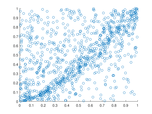
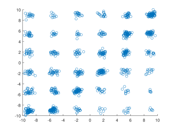
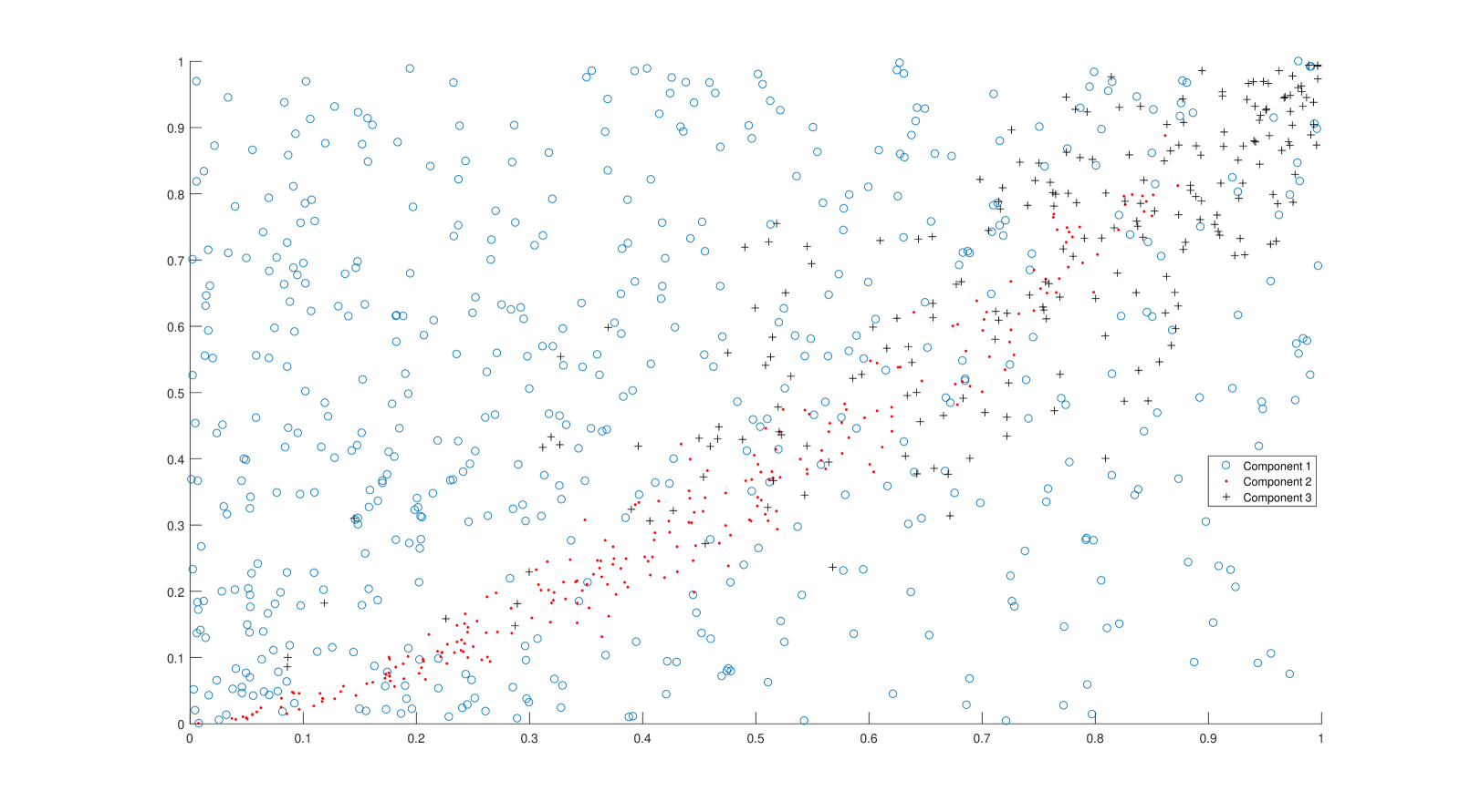
Figure 1. top left panel: An example of a draw from the non-exchangeable copula; top right panel: Original data; bottom left panel: An MCMC draw of the mixture indicators. Each of the components is labelled with a different color

$R$	2	3	4	5
Marg. Lik.	$-2613.1$	$-2609$	$-2623.8$	$-2637.6$

Table 1. Marginal likelihood estimates for different models computed using bridge sampling.

We carried out the above analysis as follows.

1. Draw a random sample $(x_{i},y_{i})$ for $i=1,\ldots,n=1000$, from the above model. Appendix B shows how to draw from the copula (1).

2. Estimate the marginal distributions using the empirical distribution functions $F_{X,n}$ and $F_{Y,n}$. Compute $z_{i}=\Phi^{-1}\circ F_{X,n}(x_{i})$ and $w_{i}=\Phi^{-1}\circ F_{Y,n}(y_{i})$ for $i=1,\ldots,n$, where $\Phi$ is the CDF of the standard normal distribution.

3. Approximate the joint distribution of $(z_{i},w_{i})$ using a mixture of multivariate normals.

4. Apply $\Phi$ to recover the copula approximation.

Step 3 can be carried out using any standard approach for estimating mixtures of multivariate normals, and we applied textbook techniques from Frühwirth-Schnatter, (2006).

We adopt a Bayesian paradigm, but a similar procedure can be carried out using a more classical approach. We repeated the model fitting for models with a different number of components and chose the model with the highest marginal likelihood. Independent multivariate normal and inverse Wishart priors are placed on the parameters of the mixture components as described in Subsection 6.3.2 in Frühwirth-Schnatter, (2006). We then ran the MCMC algorithm 6.2 from Frühwirth-Schnatter, (2006) for each model and its marginal likelihood was computed by bridge sampling. All the MCMC computations were carried out using the bayesf_version_2.0 Matlab package by Frühwirth-Schnatter, (2006).

The marginal likelihood estimates in Table 1 were obtained by estimating the copula density model

$$\sum_{r=1}^{R}\pi_{r}\frac{\phi_{\boldsymbol{\mu}_{r},\sigma_{r}I_{M}}\circ\mathfrak{F}_{H}^{-1}}{\prod_{i=1}^{M}h_{i}\circ H_{i}^{-1}},$$

specified by $H_{1},\ldots,H_{M}$ standard normal distribution functions. This is valid because we use the same estimates of the marginals of $x$ and $y$ for all the fitted mixture models.

3. Asymptotic Properties

We use the framework of Massart, (2007) to illustrate some of the asymptotic properties of estimators based on the mixtures constructed by our approach. We will first characterize the bracketing entropy numbers of the family of approximating mixtures by building on the results by Maugis and Michel, (2011), then we will use those entropy numbers to apply Massart’s framework and derive a non-asymptotic concentration inequality that will show contraction rates of Hellinger distance. Coupled with the approximation results from the previous section, the concentration inequality can be used to derive consistency of our estimators.

We will start by deriving results regarding the complexity of the family of mixture approximation. For that purpose, we will introduce some new notations. Denote by $\mathcal{F}$ the family of components of the mixture approximations, that is

$$\mathcal{F}=\left\{\frac{\phi_{\boldsymbol{\mu},\boldsymbol{\Sigma}}\circ\mathfrak{F}_{H}^{-1}}{\prod_{i=1}^{M}h_{i}\circ H_{i}^{-1}};\boldsymbol{\mu}\in[-a,a]^{M},\boldsymbol{\Sigma}=\text{diag}(\sigma_{1}^{2},...,\sigma_{M}^{2}),\sigma_{1}^{2},...,\sigma_{M}^{2}\in[\lambda_{m},\lambda_{M}]\right\}$$

where $a>0$ and $\lambda_{M}>\lambda_{m}>0$. Notice, that we choose here to use diagonal matrices instead of scaled identity matrices for the covariance matrices of the components. The following results do not change by replacing $\Sigma$ with $\sigma I_{M}$.

Further, denote by $\mathcal{S}_{R}$ the family of mixtures with components in $\mathcal{F}$, that is

$$\mathcal{S}_{R}=\left\{\sum_{r=1}^{R}\pi_{r}f_{r};f_{r}\in\mathcal{F},(p_{1},...,p_{r},...,p_{R})\in\mathcal{P}_{R-1}\right\}$$

where $\mathcal{P}_{R-1}$ is the $(R-1)$-dimensional simplex, and where $f_{r}$ obviously are densities of the form $\frac{\phi_{\boldsymbol{\mu}_{r},\Sigma_{r}}\circ\mathfrak{F}_{H}^{-1}}{\prod_{i=1}^{M}h_{i}\circ H_{i}^{-1}}$.

We are interested in characterizing the complexity of the family $\mathcal{S}_{R}$ through bracketing entropy in order to derive further asymptotic properties.

If one defines the Hellinger distance by $d_{H}$ and let $\varepsilon>0$, then the bracketing entropy $\mathcal{H}_{[]}(\varepsilon,\mathcal{S}_{R},d_{H})$ is the logarithm of $\varepsilon$-bracketing covering number $\mathcal{N}_{[]}(\varepsilon,\mathcal{S}_{R},d_{H})$ with respect to $d_{H}$ defined as the minimum number of brackets $[c_{l},c_{u}]$ covering $\mathcal{S}_{R}$, that is, given $\varepsilon$, there exists $N=\mathcal{N}_{[]}(\varepsilon,\mathcal{S}_{R},d_{H})$ different functions $c_{l1},...,c_{lN}$ and $c_{u1},...,c_{uN}$ such that $d_{H}(c_{lj},c_{uj})<\varepsilon$ for every $j=1,...,N$ and furthermore, for every $c\in\mathcal{S}_{R}$, there exists $j$ such that $c_{lj}<=c<=c_{uj}$. See e.g. Van der Vaart et al., (1996) or Kosorok, (2008) for further details.

Proposition 1.

For any $\varepsilon\in(0,1]$, and given the constant $K=\frac{5}{8}\left(1-2^{-\frac{1}{4}}\right)$, then

$$\mathcal{N}_{[]}(\varepsilon,\mathcal{F},d_{H})\leq 2^{\frac{11M}{2}}M^{2M}\left(a\frac{\lambda_{M}}{\lambda_{m}}\sqrt{\frac{1}{c\lambda_{m}}}\right){}^{M}\left(\frac{1}{\varepsilon}\right)^{2M},$$

which directly implies the $\varepsilon$-bracketing entropy $\mathcal{H}_{[]}(\varepsilon,\mathcal{S}_{R},d_{H})$ can be bounded above by the sum of a constant $K=K(R,M,a,\lambda_{m},\lambda_{M})$ and a term involving $\log(1/\varepsilon)$, that is

$$\mathcal{H}_{[]}(\varepsilon,\mathcal{S}_{R},d_{H})\leq K+R(2M+1)\log\left(\frac{1}{\varepsilon}\right)$$

In this section, we show the results under the setting of known margins. Assume we have an i.i.d. sample $(\boldsymbol{u}_{1},\ldots,\boldsymbol{u}_{n})$ from a copula that has no singular component, and that has density $c_{0}$ with respect to Lebesgue’s measure and where $\boldsymbol{u}_{i}\in\mathbb{R}^{M}$ for $i=1,\ldots,n$. Let

$$\text{KL}(c_{0},c)=\int\log\left(\frac{c_{0}(x)}{c(x)}\right)c(x)\mathrm{d}x,$$

be the Kullback-Leibler divergence between the the true copula $c_{0}$ and copula $c$. Indexing models in $\mathcal{S}_{R}$ by the number of components in the mixture $R$ and the dimension $M$, we are interested in estimators $\hat{c}$ minimizing the penalized contrast function

$$\text{crit}(R,M)=\gamma_{n}(c)+\text{pen}(R)$$

with respect to $c$ where $\gamma_{n}(c)=-\frac{1}{n}\sum_{i=1}^{N}\log(c(\boldsymbol{u}_{i}))$, and where $\text{pen}(R,M)$ is a penalty function depending on $R$ and $M$. Optimizing over $c\in\mathcal{S}_{R}$ and using Massart, (2007) theorem 7.11 as illustrated in Maugis and Michel, (2011) theorem 1.1, we can prove the following result.

Theorem 5.

Given two absolute constants $K_{1}$ and $K_{2}$, given the constant $K=K(M,a,\lambda_{m},\lambda_{M})$ and given the penalty function satisfying the inequality

$$\text{pen}(R)\geq K_{1}\frac{R(2M+1)}{n}\left(1+2K^{2}+\log\left(\frac{1}{1\wedge\frac{R(2M+1)}{n}K^{2}}\right)\right),$$

there exists a model given by $\hat{R}$ that minimizes

$$\text{crit}(R)=\gamma_{n}(\hat{c}_{\hat{R}})+\text{pen}(R)$$

and the estimator $\hat{c}_{\hat{R}}$ satisfies the inequality

$$E\left[d^{2}_{H}(c_{0},\hat{c}_{\hat{R}})\right]<K_{2}\left[\inf_{R}(\text{KL}(c_{0},\mathcal{S}_{R})+\text{pen}(R))+\frac{1}{n}\right]$$

where $\text{KL}(c_{0},\mathcal{S}_{R})=\inf_{c\in\mathcal{S}_{R}}\text{KL}(c_{0},c)$.

The theorem can be specialized to hold over a compact set that is a proper subset of $[0,1]^{M}$ in case $c_{0}$ is unbounded.

4. Mixtures of Archimedean copulas

Section 4.1 summarizes some properties of Archimedean copulas and their mixtures. These properties are used in section 4.2 to derive some approximation properties of mixtures of Archimedean copulas.

4.1. Characterization of Archimedean copulas

Let $G$ be an Archimedean copula, that is a copula of the form

(2) $$G({\boldsymbol{u}})=\varphi\left(\sum_{m=1}^{M}\varphi^{-1}(u_{m})\right),\quad\text{where}\quad{\boldsymbol{u}}=(u_{1},\dots,u_{M}),$$

and $\varphi$ is a completely monotone function. The stochastic representation of an Archimedean copula asserts that if a vector of uniform random variables $\boldsymbol{U}=(U_{1},\ldots,U_{M})$ is distributed according to some Archimedean copula distribution, then there exists a random variable $D$ with positive support such that

(3) $$\varphi(t)=E(e^{-Dt})$$

and such that $U_{1},\ldots,,U_{M}$ are conditionally independent given $D$. See for instance Hofert, (2011) for more details about sampling Archimedean copulas and for additional references.

This means that given either the functional form in equation (2) or the stochastic representation in equation (3) based on $D$, the distribution of $U_{1},\ldots,U_{M}$ is exchangeable. That is, given any permutation $\sigma$ of the set $\{1,\ldots,M\}$, the distributions of $U_{1},\ldots,U_{M}$ and $U_{\sigma(1)},\ldots,U_{\sigma(M)}$ are identical.

If $G_{1},\ldots,G_{R}$ are Archimedean copulas, then $G(\boldsymbol{u}):=\pi_{1}G_{1}(\boldsymbol{u})+\cdots+\pi_{R}G_{R}(\boldsymbol{u})$ is a mixture of Archimedean copulas, and it is immediate that it is exchangeable.

For additional details about the construction of Archimedean copulas, see for instance McNeil and Nešlehová, (2009), Hofert, (2011), Mai and Scherer, (2012) or Joe, (2014).

4.2. Approximation properties of a mixture of Archimedean copulas.

Proposition 2 shows that a mixture of Archimedean copulas $G$ is incapable of approximating arbitrarily well any copula $C$ that is not exchangeable. To construct an example, we need to find a copula that is not exchangeable. Given that $G$ is exchangeable, we need to find points in $(0,1)^{M}$ that are separated by $C$, but not by $G$.

There are many non-exchangeable copulas. For instance, a typical Gaussian copula in three dimensions or more is non-exchangeable. Even in 2 dimensions, Durante, (2009) constructs several bivariate copulas that are non-exchangeable.

Proposition 2.

Let $c$ be the copula density of some non-exchangeable random vector. Then there exists an $\varepsilon>0$ such that for all $R\in\mathbb{N}$, every $\pi=(\pi_{1},\ldots,\pi_{R})$ in the $R$-simplex and every possible set of Archimedean copula densities $g_{1},\ldots,g_{R}$,

$$\left\|c-\sum_{r=1}^{R}\pi_{r}g_{r}\right\|\geqslant\varepsilon>0,$$

for the $L_{\infty}$ norm. If $c$ is also continuous, then the result also holds for the $L_{1}$ norm.

In proposition 2 and below, we define the $L_{\infty}$ norm for $f:(0,1)^{M}\rightarrow\mathbb{R}$ as $\|f\|:=\sup_{\boldsymbol{u}\in(0,1)^{M}}|f(u)|$.

5. Mixtures of Elliptical copulas

An elliptical copula is the copula of a random vector that has an elliptical distribution. Section 5.1 describes some of the properties of elliptical copulas and section 5.2 derives some of their approximation properties.

5.1. Characterization of elliptical copulas

Definition of an elliptical copula

An elliptical copula is the copula of a vector random variable $\boldsymbol{X}$ that is elliptically distributed. The $M$-dimensional random vector $\boldsymbol{X}$ is called elliptically distributed with location $\boldsymbol{\mu}\in\mathbb{R}^{M}$ and scale matrix $\boldsymbol{\Sigma}$, where $\boldsymbol{\Sigma}$ is a symmetric and positive semi-definite matrix, if

$$\boldsymbol{X}\mathop{=}\limits^{d}\boldsymbol{\mu}+\boldsymbol{A}^{\prime}\boldsymbol{Y},$$

where $\boldsymbol{Y}$ is some spherically distributed random vector and $\boldsymbol{\Sigma}=\boldsymbol{A}^{\prime}\boldsymbol{A}$. $\bf\Sigma$ also admits the variance-correlation decomposition

$$\boldsymbol{\Sigma}=\boldsymbol{SRS},$$

where $\boldsymbol{R}$ is a correlation matrix and $\boldsymbol{S}$ is a diagonal matrix having standard deviations on the main diagonal.

Example: Gaussian copula

The simplest example of an elliptical distribution is the multivariate normal, $\boldsymbol{X}\sim\mathcal{N}(\boldsymbol{\mu},\boldsymbol{\Sigma})$. In this case the $L_{2}$ norm of $\boldsymbol{Y}$ is distributed as a chi-squared with $M$ degrees of freedom.

Let $F$ be the cdf of an $M\times 1$ random vector, with marginal cdf’s $F_{1},\dots,F_{M}$. We define $\mathfrak{F}_{F}:\mathbb{R}^{M}\rightarrow(0,1)^{M}$ as $\mathfrak{F}_{F}(\boldsymbol{x}):=\left(F_{1}(x_{1}),\dots,F_{M}(x_{M})\right)$ In particular, if $F_{X}(\boldsymbol{x})$ is the CDF of $\boldsymbol{X}\sim\mathcal{N}(\boldsymbol{\mu},\boldsymbol{\Sigma})$, then $\mathfrak{F}_{F_{X}}$ is distributed as a Gaussian copula with correlation matrix $\boldsymbol{R}$.

We now show that the distribution of $\mathfrak{F}_{F_{X}}$ is invariant under linear transformations, where, without loss of generality, we assume that $\boldsymbol{\Sigma}$ is positive definite. Let $f_{X}(\boldsymbol{x})$ be the density function of $\boldsymbol{X}$. Then, the characteristic function of $\mathfrak{F}_{F_{X}}$ is

$$\mathfrak{M}(\boldsymbol{t}) = \int_{\mathbb{R}^{M}}{\rm e}^{i\langle\mathfrak{F}_{F_{X}},\boldsymbol{t}\rangle}f_{X}(\boldsymbol{x})\mathrm{d}\boldsymbol{x}$$

$$= \int_{\mathbb{R}^{M}}{\rm e}^{i\langle\mathfrak{F}_{F_{Z}},\boldsymbol{t}\rangle}f_{Z}(\boldsymbol{z})\mathrm{d}\boldsymbol{z}$$

by the change of variable $\boldsymbol{x}=\boldsymbol{Sz}+\boldsymbol{\mu}$. Clearly, only the correlation matrix $\boldsymbol{R}$ is identified, but not the location and scale parameters $\boldsymbol{\mu}$ and $\boldsymbol{S}$.

Remark 1.

We note that the identification properties derived above for a Gaussian copula extend immediately to any elliptical copula.

5.2. Approximation properties of mixtures of elliptical copulas

Mixtures of elliptical copulas cannot always approximate an arbitrary copula $C$. The key concept we will use to construct a counterexample of why the approximation breaks down is that of radial symmetry.

Definition of radial symmetry

Let $\boldsymbol{1}_{M}$ be the vector of ones in the unit $M$-cube. A copula $G$ is said to be radially symmetric if given any $\boldsymbol{u}\in(0,1)^{M}$, then $G(\boldsymbol{u})=G(\boldsymbol{1}_{M}-\boldsymbol{u})$.

If a copula $C$ is not radially symmetric, then it cannot be approximated by a mixture of radially symmetric copulas because any such mixture would also be radially symmetric and thus cannot separate points on $(0,1)^{M}$ that are separated by $C$.

Proposition 3 shows that any elliptical copula is radially symmetric and hence so is a mixture of elliptical copulas.

Proposition 3.

1. If $G$ is an elliptical copula, then $G$ is radially symmetric.

2. Suppose that $G=\pi_{1}G_{1,\boldsymbol{R}_{1}}+\cdots+\pi_{R}G_{1,\boldsymbol{R}_{R}}$ is a mixture of radially symmetric copulas. Then, $G$ is radially symmetric.

Remark 2.

It is interesting to note that radial symmetry fails in the case of a finite mixture of elliptical distributions because when each component of the mixture is radially symmetric around a different point $\boldsymbol{\mu}_{r}\in\mathbb{R}^{M}$, then the radial symmetry fails overall unless the following equalities hold $\boldsymbol{\mu}_{1}=\boldsymbol{\mu}_{2}=\cdots=\boldsymbol{\mu}_{R}=\boldsymbol{\mu}$ for some $\boldsymbol{\mu}\in\mathbb{R}^{M}$.

Proposition 4 shows that a mixture of Gaussian copulas is incapable of approximating an arbitrary copula $C$. All we need for a counterexample is a copula that is not radially symmetric.

Proposition 4.

Let $c$ be the copula density of a random vector that is not radially symmetric. Then there exists $\varepsilon>0$ such that for all $R\in\mathbb{N}$, every $\pi=(\pi_{1},\ldots,\pi_{R})$ in the $R$-simplex and every possible set of elliptical densities $g_{1},\ldots,g_{R}$,

$$\left\|c-\sum_{r=1}^{R}\pi_{r}g_{r}\right\|\geqslant\varepsilon>0,$$

for the $L_{\infty}$ norm. If $c$ is continuous, then the result also holds for the $L_{1}$ norm.

6. Empirical illustration: Application to the dependence between large financial firms

We follow Section 4 of Oh and Patton, (2013) using the same data and fit our flexible approximation to a copula that models the dependence between seven large financial institutions (Bank of America, Citigroup, Bank of New York, Goldman Sachs, J.P. Morgan, Wells Fargo and Morgan Stanley) over the period 2000-12-25 to 2011-01-05 with a total of 2521 observations. We show that our approach provides a better fit and is more parsimonious.

Let $r_{i,t},i=1,\dots,7$, be the return for the $i$th firm at time $t$, and $r_{m,t}$ the return on the S&P 500 index at time $t$. Oh and Patton, (2013) fit the following model to the data using simulated method of moments estimation.

$$r_{i,t} =\phi_{0,i}+\phi_{1,i}r_{i,t-1}+\phi_{2,i}r_{m,t-1}+\varepsilon_{i,t},\quad\varepsilon_{i,t}=\sigma_{i,t}\eta_{i,t}$$

$$\sigma_{i,t}^{2} =\omega_{i}+\beta_{i}\sigma_{i,t-1}^{2}+\alpha_{1,i}\varepsilon_{i,t-1}^{2}+\gamma_{1,i}\varepsilon_{i,t-1}^{2}\mathbbm{1}(\varepsilon_{i,t-1}\leqslant 0)$$

$$+\alpha_{2,i}\varepsilon_{m,t-1}^{2}+\gamma_{2,i}\varepsilon_{m,t-1}^{2}\mathbbm{1}(\varepsilon_{m,t-1}\leqslant 0)$$

$$r_{m,t} =\phi_{0m}+\phi_{1m}r_{m,t-1}+\varepsilon_{m,t},\varepsilon_{m,t}=\sigma_{m,t}\eta_{m,t}$$

$$\sigma_{m,t}^{2} =\omega_{m}+\beta_{m}\sigma_{m,t-1}^{2}+\alpha_{1,i}\varepsilon_{m,t-1}^{2}+\gamma_{m}\varepsilon_{m,t-1}^{2}\mathbbm{1}(\varepsilon_{m,t-1}\leqslant 0)$$

where $i=1,\ldots,7$, $t=1,\ldots,2521$ and where $\eta_{i,t}\sim\mathcal{N}(0,1)$. Oh and Patton, (2013) then estimate the $\eta_{i,t}$ and fit a Gaussian copula to $\widehat{\eta}_{t}=(\widehat{\eta}_{1t},\dots,\widehat{\eta}_{7t})^{{\it{\tiny T}}}$ to study the joint dependence of the stock returns.

Let $u_{i,t}=\Phi(\eta_{i,t})$, where $\Phi$ is the cumulative distribution function of a standard normal (alternatively let $v_{i,t}=F_{T}(\eta_{i,t})$, where $F_{T}$ is the empirical distribution function). We then fitted two kinds of models to $\boldsymbol{u}$ (or $\boldsymbol{v})$

1. Mixture I. A mixture of Gaussian copulas $\sum_{r=1}^{R}\pi_{r}c(\cdot,\boldsymbol{C}_{r})$, where the $\boldsymbol{C}_{r}$ are correlation matrices.

   The number of parameters in this model is $R\frac{M(M-1)}{2}+R-1$ where $M=7$.

2. Mixture II. A mixture of normals to $\Phi^{-1}(v_{i,t})$ and then recover the copula.

   The number of parameters in this model is $R\frac{M(M+3)}{2}+R-1-2M$. The $-2M$ term arises in the last expression occurs because when in fitting a copula, $M$ means and $M$ variances are not determined.

We note that Mixture I with $R=1$ is the Oh and Patton, (2013) approach.

Table 2. BIC values for the mixture of Gaussian copula and approximating mixture for estimating the distribution of $\eta_{t}$ flexibly.

# components	Mixture of Gaussian copulas	Approximating mixture
1	36374	36374
2	$-12912$	$-17146$
3	$-12786$	$-16930$
4	$-12660$	$-16714$

Table 2 reports the BIC values for each of the 4 models for each of Mixture I and Mixture 2. The table shows that a Gaussian copula provides an inadequate fit and the mixture of $R=2$ Gaussian copulas provides the best fit if we use a mixture of Gaussian copulas. The table also shows that the best approximating mixture has two components (BIC of $-17146$) and provides a far better fit than the best mixture of Gaussian copulas (BIC of $-12912$). If we take all models as equally likely, and use $\exp(-\frac{1}{2}BIC)$ as an estimate of the marginal likelihood of each model under flat priors, then the ratio of the posterior probability of the best approximating model to the Gaussian copula models is $\exp(26670)$ and the ratio of the best approximating model to the best approximation by a mixture of Gaussian copulas is $\exp(2117)$.

7. Conclusion

Our article provides fundamental tools for approximating any copula arbitrarily well and uses these to propose a practical family of mixtures to provide such an approximation. We can then use this approximation to construct a practical copula-based approach for approximating any multivariate distribution arbitrarily well. Such a copula approach for universally approximating multivariate distributions is attractive as it allows us to control the degree of approximation of the marginal distributions as well as providing a flexible way of approximating the joint dependence. Furthermore, the approach is easy to implement and satisfies good asymptotic properties. Thus, our approach can provide an attractive alternative to approximating multivariate distributions by a mixture of normals. We also study the approximation properties of mixtures of Gaussian copulas or mixtures of Archimedean copulas and show that neither family of mixtures can approximate a general copula arbitrarily well.

Furthermore, the universal approximation results proved in this paper are theoretical and of a probabilistic/analytic nature, and thus are essential for further statistical analysis of the problem. In fact, they constitute standard density results (like showing that a continuous function under certain assumptions can be approximated by polynomials and splines) that are a cornerstone for all sieve-based non-parametric estimation techniques and are a pre-requisite for further analysis. This means that they bring the whole machinery of mixture modeling to bear on the problem of non-parametric estimation of copulas. Given that the results show it is legitimate to use our mixture based model under certain conditions to approximate copulas, then the standard mixture machinery can then be legitimately used to estimate that model and hence the copula. In particular, if one wants to use nonparametric copula estimation using sieves built from mixtures, or Dirichlet process mixtures in a Bayesian setting, then the results are both a pre-requisite and foundational. See, for example, the way sieves are constructed in say Shen, (1997) or Chen, (2007).

Appendix A Proofs

Theorem 1.

The proof follows from Bacharoglou, (2010). See in that paper theorem 2.4 for the compact support approximation case, corollary 2.5(2) for the $L_{1}$ approximation case, and corollary 2.5(3) for the $L_{\infty}$ approximation case. ∎

Theorem 2 .

We first prove the theorem for the $L_{1}$ norm. Let $U$ be a random variable with density $g$. Applying the transformation $X=H^{-1}(U)$ yields an absolutely continuous random variable with support on the whole real line with density $f=h\cdot(g\circ H^{-1})$. Furthermore, $f$ is clearly both continuous and bounded. We can apply theorem 1 to get the following approximation property.

For every $\varepsilon>0$, there exists a sequence $(\alpha_{n})_{n\in\mathbb{N}}$ in $\mathcal{A}^{+}$ and an integer $R$ such that in the enumeration $(\phi_{n})_{n}$ specified by $\phi_{\mu,\frac{1}{k}}(x)$, where $k\in\mathbb{N}$, $\mu\in\mathbb{Q}$, the convex combination

$$\sum_{r=1}^{R}\pi_{r}\phi_{r},\quad\text{with}\quad\pi_{r}:=\frac{\alpha_{r}}{\sum_{r^{\prime}=1}^{R}\alpha_{r^{\prime}}},$$

is arbitrarily close to $f$. Denoting the normalized weights by $\pi_{r}$ and the normal densities parameters in the enumeration by $\mu_{1},\ldots,\mu_{R},\sigma_{1},\ldots,\sigma_{R}$ yields the required result.

$$\left\|f-\sum_{r=1}^{R}\pi_{r}\phi_{\mu_{r},\sigma_{r}}\right\|<\varepsilon.$$

Finally, applying the transformation $H$ yields

$$\varepsilon >\left\|f-\sum_{r=1}^{R}\pi_{r}\phi_{\mu_{r},\sigma_{r}}\right\|_{1}$$

$$=\int_{-\infty}^{\infty}\left|f(x)-\sum_{r=1}^{R}\pi_{r}\phi_{\mu_{r},\sigma_{r}}(x)\right|\mathrm{d}x$$

$$=\int_{0}^{1}\left|\frac{f\circ H^{-1}}{h\circ H^{-1}}(u)-\sum_{r=1}^{R}\pi_{r}\frac{\phi_{\mu_{r},\sigma_{r}}\circ H^{-1}}{h\circ H^{-1}}(u)\right|\mathrm{d}u$$

$$=\int_{0}^{1}\left|g(u)-\sum_{r=1}^{R}\pi_{r}\frac{\phi_{\mu_{r},\sigma_{r}}\circ H^{-1}}{h\circ H^{-1}}(u)\right|\mathrm{d}u$$

$$=\left\|g-\sum_{r=1}^{R}\pi_{r}\frac{\phi_{\mu_{r},\sigma_{r}}\circ H^{-1}}{h\circ H^{-1}}\right\|.$$

We now consider the $L_{\infty}$ case. Suppose the result does not hold for this case. Then, there exists an $\varepsilon>0$, such that for any $R\in\mathbb{N}$, $(\pi_{1},\ldots,\pi_{R})\in\Delta_{R}$ (the $R$-simplex), $\mu_{1},\ldots,\mu_{R}\in\mathbb{R}$ and $\sigma_{1},\ldots,\sigma_{R}\in(0,\infty)$ such that

$$\left\|g-\sum_{r=1}^{R}\pi_{r}\phi_{\mu_{r},\sigma_{r}}\circ H^{-1}\right\|_{\infty}\geq\varepsilon.$$

This implies that the result of theorem does not hold for the $L_{1}$ norm as $g(\cdot)$ is continuous, providing a contradiction. ∎

Theorem 3 .

We prove the theorem for the $L_{1}$ norm. The proof for the $L_{\infty}$ norm is similar to that in the proof of theorem 2. Applying the inverse transformation $\mathfrak{F}_{H}^{-1}:[0,1]^{M}\rightarrow\mathbb{R}^{M}$ yields an $\mathbb{R}^{M}$ random vector with density

$$f(\boldsymbol{x})=c(\mathfrak{F}_{H}(\boldsymbol{x}))\prod_{j=1}^{M}h_{j}(x_{j}).$$

The function $f$ is trivially in $L_{1}$ (with respect to Lesbesgue measure) as it is the density of an absolutely continuous random vector. Furthermore $f\in L_{\infty}\cap C(\mathbb{R}^{M})$ because it is bounded and continuous. Suppose $\varepsilon>0$ is given. Applying theorem 1 to $f$, there exists a sequence $(\alpha_{n})_{n\in\mathbb{N}}$ in $\mathcal{A}^{+}$ and an integer $R$ such that in the enumeration $(\phi_{n})_{n}$ specified by $\phi_{\frac{1}{k}}(\boldsymbol{x}-\boldsymbol{\mu})$ where $k\in\mathbb{N}$, $\boldsymbol{\mu}\in\mathbb{Q}^{M}$, the convex combination

$$\sum_{r=1}^{R}\pi_{r}\phi_{r},\quad\text{where}\quad\pi_{r}:=\frac{\alpha_{r}}{\sum_{r^{\prime}=1}^{R}\alpha_{r}^{\prime}}.$$

If the mean vector and variance parameters corresponding to the enumeration are $\boldsymbol{\mu}_{1},\ldots,\boldsymbol{\mu}_{R},\sigma_{1},\ldots,\sigma_{R}$, then

$$\left\|f-\sum_{r=1}^{R}\pi_{r}\phi_{\boldsymbol{\mu}_{r},\sigma_{r}\boldsymbol{I}_{m}}\right\|<\varepsilon.$$

Explicitly writing the previous expression and applying the transformation $H$ yields

$$\varepsilon > \int_{\mathbb{R}^{M}}\left|f(\boldsymbol{x})-\sum_{r=1}^{R}\pi_{r}\phi_{\boldsymbol{\mu}_{r},\sigma_{r}\boldsymbol{I}_{m}}(\boldsymbol{x})\right|\mathrm{d}\boldsymbol{x}$$

$$= \int_{(0,1)^{M}}\left|c(\boldsymbol{u})-q_{R}(\boldsymbol{u})\right|\mathrm{d}\boldsymbol{u}$$

with $q_{R}(\boldsymbol{u}):=\sum_{r=1}^{R}\pi_{r}\frac{\phi_{\boldsymbol{\mu}_{r},\sigma_{r}\boldsymbol{I}_{m}}\circ\mathfrak{F}_{H}^{-1}}{\prod_{i=1}^{M}h_{i}\circ H_{i}^{-1}}(\boldsymbol{u})$. ∎

Corollary 1.

We need the following standard result that is adapted from Devroye and Lugosi, (2012).

Let $T$ be a Borel measurable mapping from $\mathbb{R}^{M}$ into $\mathbb{R}^{L}$ and let $f$ and $g$ be the density functions of two arbitrary $\mathbb{R}^{M}$ random vectors and $f_{T}$ and $g_{T}$ be respectively the densities of the mapped random vectors then

$$\|f-g\|_{1}\geqslant\|f_{T}-g_{T}\|_{1}$$

. This is proved as follows. Let $f$ and $g$ be the densities of $X$ and $Y$ respectively.

$$\|f-g\|_{1} = 2\sup_{A\in\mathcal{B}(\mathbb{R}^{M})}|\Pr\{X\in A\}-\Pr\{Y\in A\}|$$

$$\geqslant 2\sup_{A\in\mathcal{B}(\mathbb{R}^{L})}|\Pr\{T(X)\in A\}-\Pr\{T(Y)\in A\}|$$

$$= \int_{\mathbb{R}^{M}}|f_{T(X)}-g_{T(X)}|\mathrm{d}\mu,$$

where the first line is Scheffé’s identity (theorem 5.1 in Devroye and Lugosi, (2012)) and the second line follows from theorem 5.2 in the same reference.

A simple application of that result now yields our corollary. Consider the transformation $T(\boldsymbol{u}):=u_{i}$. The proof for the $L_{1}$ norm now follows immediately. The proof for the $L_{\infty}$ norm follows because the marginals of $c$ are uniform. ∎

Corollary 2 .

Let $\boldsymbol{V}=\mathfrak{F}_{F}(\boldsymbol{X})$, let $F_{V}$ be the CDF of $\boldsymbol{V}$ with marginals $F_{V,i}$ and let $C_{V}$ be the copula of $\boldsymbol{V}$. Let $W_{i}:=F_{V,i}(V_{i}),i=1,\dots,M$, $\boldsymbol{W}:=(W_{1},\dots,W_{M})$. Then,

$$w_{i} =F_{V,i}(v_{i})=G_{i}(F_{i}^{-1}(v_{i}))=G_{i}(F_{i}^{-1}(F_{i}(x_{i})))=G_{i}(x_{i}).$$

The characteristic function of $\boldsymbol{W}$ is

$$\mathfrak{M}(\boldsymbol{t}) =\int_{\mathbb{R}^{M}}\exp\left(i\left(\sum_{i=1}^{M}t_{i}w_{i}\right)\right)g(\boldsymbol{x})\mathrm{d}\boldsymbol{x}=\int_{\boldsymbol{R}^{M}}\exp\left(i\left(\sum_{i=1}^{M}t_{i}G_{i}(x_{i})\right)\right)g(\boldsymbol{x})\mathrm{d}\boldsymbol{x},$$

which is the characteristic function of $C_{G}$. ∎

Theorem 4 .

Assume there exists $f_{\varepsilon}$ such that $|c-f_{\varepsilon}|<\varepsilon$.

Let $f_{1},\ldots,f_{M}$ and $F_{1},\ldots,F_{M}$ be respectively the marginal densities and distribution functions of $f_{\varepsilon}$ and let $f_{\pi}=f_{1}\cdots f_{M}$ be the product of the marginal densities.

Let $v:=v(u)=(F_{1}^{-1}(u_{1}),\ldots,F_{M}^{-1}(u_{M}))$ be the point in $[0,1]^{M}$ that results by applying the transformation $F_{m}^{-1}$ to each coordinate $u_{m}$ of $u=(u_{1},\ldots,u_{M})$.

Thus we an write $f_{\varepsilon}(v)=f_{\pi}(u)c_{f}(u)$ where $c_{f}$ is the copula density of $f_{\varepsilon}$.

It is well know that the Kullback-Leibler divergence satisfies the following inequality with respect to the $L_{1}$ norm

$$\|c_{f}-c\|_{1}^{2}\leqslant 2KL(c_{f},c)$$

so that in order to bound the $L_{1}$ norm from above, we will try to bound the Kullback-Leibler divergence

$$KL(c_{f},c) = \int\log\left(\frac{c_{f}(u)}{c(u)}\right)c_{f}(u)\mathrm{d}u$$

$$= \int\log\left(\frac{c_{f}(u)}{c(u)}\times\frac{f_{\pi}(u)}{f_{\pi}(u)}\right)c_{f}(u)\mathrm{d}u$$

$$= \int\log\left(\frac{f_{\varepsilon}(v)}{c(u)}\right)c_{f}(u)\mathrm{d}u-\int\log(f_{\pi}(u))c_{f}(u)\mathrm{d}u$$

$$= \int\log\left(\frac{f_{\varepsilon}(v)}{c(u)}\times\frac{f_{\varepsilon}(u)}{f_{\varepsilon}(u)}\right)c_{f}(u)\mathrm{d}u-\int\log(f_{\pi}(u))c_{f}(u)\mathrm{d}u$$

$$= \int\log\left(\frac{f_{\varepsilon}(u)}{c(u)}\right)c_{f}(u)\mathrm{d}u+\int\log\left(\frac{f_{\varepsilon}(v)}{f_{\varepsilon}(u)}\right)c_{f}(u)\mathrm{d}u-\int\log(f_{\pi}(u))c_{f}(u)\mathrm{d}u$$

so that

$$KL(c_{f},c)\leqslant\left|\int\log\left(\frac{f_{\varepsilon}(u)}{c(u)}\right)c_{f}(u)\mathrm{d}u\right|+\left|\int\log\left(\frac{f_{\varepsilon}(v)}{f_{\varepsilon}(u)}\right)c_{f}(u)\mathrm{d}u\right|+\left|\int\log(f_{\pi}(u))c_{f}(u)\mathrm{d}u\right|$$

The first term can be made arbitrarily small by theorem 3. The last term can be made arbitrarily small by corollary 1, as $f_{\pi}(u)$ can be made arbitrarily close to 1. Finally, if we assume that the transformation $H$ has a continuous density on $\mathbbm{R}$ (Assuming that $H\in C_{1}(\mathbbm{R})$), then $f_{\varepsilon}(v)$ can be made arbitrarily close to $f_{\varepsilon}(u)$ by the continuity of $f_{\varepsilon}$ as $u$ can be made arbitrarily close to $v$ by corollary 1.

∎

Proposition  1 .

The proof follows closely the argument of theorem 2.1 Maugis and Michel, (2011). For that argument to hold, we need to prove two additional results that are necessary to check for $\mathcal{F}$. As the argument requires the construction of a lattices over the parameters of $\mathcal{F}$, given that we are not dealing with multivariate normal densities, but with multivariate normal densities applied after some monotonic transformations, we need to check that the brackets constructed for the multivariate normal density case can be constructed in the same here, given both the multivariate normal density family and $\mathcal{F}$ share the same parameter space.

The first result is that proposition C.1 in Maugis and Michel, (2011) dealing with an upper bound on the ratio of two normal densities also hold in the case of densities in $\mathcal{F}$ because the denominators in the densities expressions simplify and because $[0,1]^{M}\subset\mathbb{R}^{M}$.

The second result is that proposition C.3 in Maugis and Michel, (2011) dealing with the Hellinger distance between the upper and lower functions in the bracket can be computed in the same way. Please note that

$$d^{2}_{H}(\phi_{\boldsymbol{\mu}_{1},\boldsymbol{\Sigma}_{1}},\phi_{\boldsymbol{\mu}_{2},\boldsymbol{\Sigma}_{2}}) = 2-2\int_{\mathbb{R}^{M}}\sqrt{\phi_{\boldsymbol{\mu}_{1},\boldsymbol{\Sigma}_{1}}(\boldsymbol{x})\phi_{\boldsymbol{\mu}_{2},\boldsymbol{\Sigma}_{2}}(\boldsymbol{x})}hd\boldsymbol{x}$$

$$= 2-2\int_{[0,1]^{M}}\sqrt{\frac{\phi_{\boldsymbol{\mu}_{1},\boldsymbol{\Sigma}_{1}}\circ\mathfrak{F}_{H}^{-1}(\boldsymbol{u})}{\prod_{i=1}^{M}h_{i}\circ H_{i}^{-1}(u_{i})}\times\frac{\phi_{\boldsymbol{\mu}_{2},\boldsymbol{\Sigma}_{2}}\circ\mathfrak{F}_{H}^{-1}(\boldsymbol{u})}{\prod_{i=1}^{M}h_{i}\circ H_{i}^{-1}(u_{i})}}d\boldsymbol{u}$$

$$= d^{2}_{H}\left(\frac{\phi_{\boldsymbol{\mu}_{1},\boldsymbol{\Sigma}_{1}}\circ\mathfrak{F}_{H}^{-1}}{\prod_{i=1}^{M}h_{i}\circ H_{i}^{-1}},\frac{\phi_{\boldsymbol{\mu}_{2},\boldsymbol{\Sigma}_{2}}\circ\mathfrak{F}_{H}^{-1}}{\prod_{i=1}^{M}h_{i}\circ H_{i}^{-1}}\right)$$

The remainder of the proof for the calculation of the bracketing entropy for $\mathcal{F}$ proceeds in the construction in the lattice in exactly same way for multivariate normal densities (proof of theorem 2.2 in Maugis and Michel, (2011)).

The calculation of the entropy for $\mathcal{S}_{R}$ proceeds from the calculation for $\mathcal{F}$ and from theorem 2 in Genovese and Wasserman, (2000).

∎

Theorem  5 .

In the statement of the theorem, $K$ is given by

$$K=\sqrt{\pi}+\sqrt{\log(18\pi e^{2})}+\sqrt{\log\left(a\sqrt{\frac{8}{c_{1}\lambda_{m}}}\right)}+\sqrt{\log\left(8\frac{\lambda_{M}}{\lambda_{m}}\right)}+\sqrt{\log\left(9\sqrt{2}M\right)}$$

The remainder proceeds in exactly the same way as the proof of theorem 2.1 in Maugis and Michel, (2011). In particular, as cited in the proof of that paper, the function $\Psi_{R}$ defined by $\Psi_{R}(\xi)=\xi\sqrt{R(2M+1)}\left\{K+\sqrt{\log\left(\frac{1}{1\wedge\xi}\right)}\right\}$ provides an upper bound for the entropy integral.

∎

Proposition 2 .

We first prove the result for the $L_{\infty}$ norm. The densities $g_{r}$ being exchangeable means that for every permutation $\sigma$ of the set $\{1,\ldots,M\}$, we have the identity $g_{r}(\boldsymbol{u})=g_{r}(\boldsymbol{u}_{\sigma})$, where $\boldsymbol{u}_{\sigma}:=(u_{\sigma(1)},\dots,u_{\sigma(M)})$. Taking convex combinations retains that symmetry. If we define $g:=\sum_{r=1}^{R}\pi_{r}g_{r}$, then $g$ is also exchangeable,

$$g(\boldsymbol{u}) =\sum_{r=1}^{R}\pi_{r}g_{r}(\boldsymbol{u})$$

$$=\sum_{r=1}\pi_{r}g_{r}(\boldsymbol{u}_{\sigma})=g(\boldsymbol{u}_{\sigma}).$$

There exists at least one $\boldsymbol{u}\in(0,1)^{M}$ and one $\sigma$ such that $c(\boldsymbol{u})\neq c(\boldsymbol{u}_{\sigma})$ because $c$ is non-exchangeable, and hence $g$ is incapable of separating some points that $c$ is capable of separating. For one of these points, define for $\eta>0$

$$\eta =|c(\boldsymbol{u})-c(\boldsymbol{u}_{\sigma})|$$

$$=|c(\boldsymbol{u})-g(\boldsymbol{u})+g(\boldsymbol{u})-g(\boldsymbol{u}_{\sigma})+g(\boldsymbol{u}_{\sigma})-c(\boldsymbol{u}_{\sigma})|$$

$$\leqslant|c(\boldsymbol{u})-g(\boldsymbol{u})|+|c(\boldsymbol{u}_{\sigma})-g(\boldsymbol{u}_{\sigma})|+|g(\boldsymbol{u})-g(\boldsymbol{u}_{\sigma})|$$

$$=|c(\boldsymbol{u})-g(\boldsymbol{u})|+|c(u_{\sigma})-g(\boldsymbol{u})|$$

$$\leqslant 2\max\{|c(\boldsymbol{u})-g(\boldsymbol{u})|,|c(\boldsymbol{u}_{\sigma})-g(\boldsymbol{u}_{\sigma})|\}$$

$$\leqslant 2\sup_{\boldsymbol{u}\in(0,1)^{M}}|c(\boldsymbol{u})-g(\boldsymbol{u})|.$$

Hence,

$$\sup_{\boldsymbol{u}\in(0,1)^{M}}|c(\boldsymbol{u})-g(\boldsymbol{u})| \geqslant \eta/2>0.$$

Choosing $\varepsilon=\eta/2$ is sufficient to prove the proposition.

Now all that is necessary is to find such an $\eta$, given that we are constructing a counter-example. For $M=2$, consider the copula (which is constructed using arguments in Durante, (2009))

$$C(u,v)=u^{1-\alpha}v^{1-\beta}[u^{-\theta\alpha}+v^{-\theta\beta}-1]^{-\frac{1}{\theta}},$$

where $\alpha,\beta\in(0,1)$ and $\theta>0$. We need to impose the constraint that either $\alpha\neq\frac{1}{2}$ or $\beta\neq\frac{1}{2}$ to get a non-exchangeable copula. In particular, picking a concrete example, let $\alpha=\frac{1}{4}$, $\beta=\frac{1}{2}$, $\theta=20$, $u=\frac{1}{3}$ and $v=\frac{2}{3}$ yields an $\eta>0.2$. Taking $\varepsilon=0.1$ yields the counterexample.

Since we are ultimately interested in approximating copula densities and not copulas themselves, it is possible to work with the copula density of the previous copula and show that we obtain $\eta>0.3$ for the same parameter values.

The proof for the $L_{1}$ norm follows from that of the $L_{\infty}$ norm because $c$ is continuous and we only need to look at a compact subset. ∎

Proposition 3 .

Proof of (i). Without loss of generality, consider the stochastic representation $\boldsymbol{X}:=\boldsymbol{A}\boldsymbol{Y},\quad\boldsymbol{U}=F(\boldsymbol{X}),$ where $\boldsymbol{Y}$ is spherically symmetric, $\boldsymbol{R}=\boldsymbol{A}^{\prime}\boldsymbol{A}$ and $F$ is the distribution of $\boldsymbol{X}$. Then $\boldsymbol{oY}\mathop{=}\limits^{d}\boldsymbol{Y}$ for any orthogonal matrix $\boldsymbol{o}$ because $\boldsymbol{Y}$ is spherically symmetric. It implies that $-\boldsymbol{X}\mathop{=}\limits^{d}\boldsymbol{X}$ and thus $\boldsymbol{1}_{M}-\boldsymbol{U}=\boldsymbol{1}_{M}-F(\boldsymbol{X})=F(-\boldsymbol{X}).$ Finally, consider a finite mixture of elliptical copulas $G=\pi_{1}G_{1,\boldsymbol{R}_{1}}+\cdots+\pi_{R}G_{1,\boldsymbol{R}_{R}}$. Each component is radially symmetric (around $\frac{1}{2}\boldsymbol{1}_{M}$) implying that $G$ is again radially symmetric. ∎

Proposition 4 .

We give the proof for the $L_{\infty}$ norm. The proof for the $L_{1}$ norm then follows from the continuity of $c$ over a compact subset. We already showed that $g=\sum_{r=1}^{R}\pi_{r}g_{r}$ is radially symmetric. The copula density $c$ being non-radially symmetric means that there exists at least one $\boldsymbol{u}\in(0,1)^{M}$, $c(\boldsymbol{u})\neq c(\boldsymbol{1}_{M}-\boldsymbol{u})$. As in the Archimedean copula case, the lack of approximation occurs because $g$ is incapable of separating some points that $c$ is capable of separating. For one of those points, define, for $\eta>0$,

$$\eta :=|c(\boldsymbol{u})-c(\boldsymbol{1}_{M}-\boldsymbol{u})|$$

$$=|c(\boldsymbol{u})-g(\boldsymbol{u})+g(\boldsymbol{u})-g(\boldsymbol{1}_{M}-\boldsymbol{u})+g(\boldsymbol{1}_{M}-\boldsymbol{u})-c(\boldsymbol{1}_{M}-\boldsymbol{u})|$$

$$\leqslant|c(\boldsymbol{u})-g(\boldsymbol{u})|+|g(\boldsymbol{u})-g(\boldsymbol{1}_{M}-\boldsymbol{u})|+|g(\boldsymbol{1}_{M}-u)-c(\boldsymbol{1}_{M}-\boldsymbol{u})|$$

$$=|c(\boldsymbol{u})-g(\boldsymbol{u})|+|g(\boldsymbol{1}_{M}-\boldsymbol{u})-c(\boldsymbol{1}_{M}-\boldsymbol{u})|$$

$$\leqslant 2\max\{|c(\boldsymbol{u})-g(\boldsymbol{u})|,|g(\boldsymbol{1}_{M}-\boldsymbol{u})-c(\boldsymbol{1}_{M}-\boldsymbol{u})|\}$$

$$\leqslant 2\sup_{\boldsymbol{u}\in(0,1)^{M}}|c(\boldsymbol{u})-g(\boldsymbol{u})|.$$

We deduce that choosing $\varepsilon=\eta/2$ is sufficient to prove the existence of the counter-example. Consider a Clayton copula in two dimensions with parameter $\theta=1$

$$c(u,v):=\frac{2uv}{(u+v-uv)^{3}}.$$

Picking $u=\frac{1}{10}$ and $v=\frac{1}{2}$ allows us to find $\eta>0.4$. ∎

Appendix B Drawing from the bivariate copula (1)

First, we note that the conditional copula distribution

$$C(u|v) = \frac{\partial}{\partial v}C(u,v)$$

$$= (1-\beta)u^{1-\alpha}v^{-\beta}[u^{-\theta\alpha}+v^{-\theta\beta}-1]^{-\frac{1}{\theta}}$$

$$+ \beta u^{1-\alpha}v^{-\beta(1+\theta)}[u^{-\theta\alpha}+v^{-\theta\beta}-1]^{-\frac{1}{\theta}-1}$$

can itself be written as a mixture with $\beta\in(0,1)$ determining the mixing probability. We can sample from this model as follows

• Draw $V$ from a uniform distribution. Set $X_{1}=F_{1}^{-1}(V)$.

• Draw another independent uniform $W$. Set $U=C^{-1}(W|V)$. Set $X_{2}=F_{2}^{-1}(U)$.

  Thus, $(U,V)$ is a draw from the copula model and $(X_{1},X_{2})$ is a draw from $f$.

References

- Bacharoglou, (2010) Bacharoglou, A. (2010). Approximation of probability distributions by convex mixtures of Gaussian measures. Proceedings of the American Mathematical Society, 138(7):2619–2628.
- Burda and Prokhorov, (2014) Burda, M. and Prokhorov, A. (2014). Copula based factorization in Bayesian multivariate infinite mixture models. Journal of Multivariate Analysis, 127:200 – 213.
- Chen, (2007) Chen, X. (2007). Large sample sieve estimation of semi-nonparametric models. Handbook of econometrics, 6:5549–5632.
- Dalal and Hall, (1983) Dalal, S. and Hall, W. (1983). Approximating priors by mixtures of natural conjugate priors. Journal of the Royal Statistical Society. Series B (Methodological), 45(2):278–286.
- Devroye and Lugosi, (2012) Devroye, L. and Lugosi, G. (2012). Combinatorial methods in density estimation. Springer.
- Durante, (2009) Durante, F. (2009). Construction of non-exchangeable bivariate distribution functions. Statistical Papers, 50(2):383–391.
- Durante and Sempi, (2015) Durante, F. and Sempi, C. (2015). Principles of copula theory. Chapman and Hall/CRC.
- Fermanian et al., (2004) Fermanian, J.-D., Radulovic, D., and Wegkamp, M. (2004). Weak convergence of empirical copula processes. Bernoulli, 10(5):847–860.
- Frühwirth-Schnatter, (2006) Frühwirth-Schnatter, S. (2006). Finite mixture and Markov switching models. Springer Science & Business Media.
- Genest et al., (2009) Genest, C., Masiello, E., and Tribouley, K. (2009). Estimating copula densities through wavelets. Insurance: Mathematics and Economics, 44(2):170 – 181.
- Genovese and Wasserman, (2000) Genovese, C. R. and Wasserman, L. (2000). Rates of convergence for the gaussian mixture sieve. The Annals of Statistics, 28(4):1105–1127.
- Hofert, (2011) Hofert, M. (2011). Efficiently sampling nested Archimedean copulas. Computational Statistics and Data Analysis, 55(1):57 – 70.
- Ishwaran and James, (2001) Ishwaran, H. and James, L. F. (2001). Gibbs sampling methods for stick-breaking priors. Journal of the American Statistical Association, 96(453):161–173.
- Joe, (2014) Joe, H. (2014). Dependence modeling with copulas. CRC Press.
- Kalli et al., (2011) Kalli, M., Griffin, J. E., and Walker, S. G. (2011). Slice sampling mixture models. Statistics and computing, 21(1):93–105.
- Kosorok, (2008) Kosorok, M. R. (2008). Introduction to empirical processes and semiparametric inference. Springer.
- Koumandos et al., (2010) Koumandos, S., Nestoridis, V., Smyrlis, Y.-S., and Stefanopoulos, V. (2010). Universal series in . Bulletin of the London Mathematical Society, 42(1):119–129.
- Lijoi, (2003) Lijoi, A. (2003). Approximating priors by finite mixtures of conjugate distributions for an exponential family. Journal of Statistical Planning and Inference, 113(2):419 – 435.
- Mai and Scherer, (2012) Mai, J.-F. and Scherer, M. (2012). Simulating copulas: stochastic models, sampling algorithms and applications. World Scientific.
- Massart, (2007) Massart, P. (2007). Concentration inequalities and model selection: Ecole d’Eté de Probabilités de Saint-Flour XXXIII-2003. Springer.
- Maugis and Michel, (2011) Maugis, C. and Michel, B. (2011). A non asymptotic penalized criterion for gaussian mixture model selection. ESAIM: Probability and Statistics, 15:41–68.
- McLachlan and Peel, (2000) McLachlan, G. and Peel, D. (2000). Mixtures of Factor Analyzers in Finite Mixture Models. John Wiley & Sons, Hoboken, NJ, USA.
- McNeil and Nešlehová, (2009) McNeil, A. J. and Nešlehová, J. (2009). Multivariate Archimedean copulas, -monotone functions and -norm symmetric distributions. The Annals of Statistics, 37(5):3059–3097.
- Oh and Patton, (2013) Oh, D. H. and Patton, A. J. (2013). Simulated method of moments estimation for copula-based multivariate models. Journal of the American Statistical Association, 108(502):689–700.
- Omelka et al., (2009) Omelka, M., Gijbels, I., and Veraverbeke, N. (2009). Improved kernel estimation of copulas: weak convergence and goodness-of-fit testing. The Annals of Statistics, 37(5B):3023–3058.
- Sancetta, (2007) Sancetta, A. (2007). Nonparametric estimation of distributions with given marginals via Bernstein-Kantorovich polynomials: L1 and pointwise convergence theory. Journal of Multivariate Analysis, 98:1376–1390.
- Sancetta and Satchell, (2004) Sancetta, A. and Satchell, S. (2004). The Bernstein copula and its applications to modeling and approximations of multivariate distributions. Econometric theory, 20(3):535–562.
- Segers, (2012) Segers, J. (2012). Asymptotics of empirical copula processes under non-restrictive smoothness assumptions. Bernoulli, 18(3):764–782.
- Shen, (1997) Shen, X. (1997). On methods of sieves and penalization. The Annals of Statistics, 25(6):2555–2591.
- Tran et al., (2014) Tran, M.-N., Giordani, P., Mun, X., Kohn, R., and Pitt, M. K. (2014). Copula-type estimators for flexible multivariate density modeling using mixtures. Journal of Computational and Graphical Statistics, 23(4):1163–1178.
- Van der Vaart et al., (1996) Van der Vaart, A. W., Wellner, J. A., van der Vaart, A. W., and Wellner, J. A. (1996). Weak convergence and and empirical processes. Springer.
- Wu et al., (2014) Wu, J., Wang, X., and Walker, S. G. (2014). Bayesian nonparametric inference for a multivariate copula function. Methodology and Computing in Applied Probability, 16(3):747–763.
- Wu et al., (2015) Wu, J., Wang, X., and Walker, S. G. (2015). Bayesian nonparametric estimation of a copula. Journal of Statistical Computation and Simulation, 85(1):103–116.
- Zeevi and Meir, (1997) Zeevi, A. J. and Meir, R. (1997). Density estimation through convex combinations of densities: Approximation and estimation bounds. Neural Networks, 10(1):99 – 109.