Spectral rigidity for spherically symmetric manifolds with boundary

Abstract.

We prove a trace formula for three-dimensional spherically symmetric Riemannian manifolds with boundary which satisfy the Herglotz condition: The wave trace is singular precisely at the length spectrum of periodic broken rays. In particular, the Neumann spectrum of the Laplace–Beltrami operator uniquely determines the length spectrum. The trace formula also applies for the toroidal modes of the free oscillations in the earth. We then prove that the length spectrum is rigid: Deformations preserving the length spectrum and spherical symmetry are necessarily trivial in any dimension, provided the Herglotz condition and a generic geometrical condition are satisfied. Combining the two results shows that the Neumann spectrum of the Laplace–Beltrami operator is rigid in this class of manifolds with boundary.

1. Introduction

We establish spectral rigidity for spherically symmetric manifolds with boundary. We study the recovery of a (radially symmetric Riemannian) metric or wave speed rather than an obstacle. To our knowledge it is the first such result pertaining to a manifold with boundary. We require the so-called Herglotz condition while allowing an unsigned curvature; that is, curvature can be everywhere positive or it can change sign, and we allow for conjugate points. Spherically symmetric manifolds with boundary are models for planets, the preliminary reference Earth model (PREM) being the prime example. Specifically, restricting to toroidal modes, our spectral rigidity result determines the shear wave speed of Earth’s mantle in the rigidity sense.

The method of proof relies on a trace formula, relating the spectrum of the manifold with boundary to its length spectrum, and the injectivity of the periodic broken ray transform. Specifically, our manifold is the Euclidean annulus $M=\bar{B}(0,1)\setminus\bar{B}(0,R)\subset{\mathbb{R}}^{n}$, $R>0$ and $n\geq 2$, with the metric $g(x)=c^{-2}(\left\lvert x\right\rvert)e(x)$, where $e$ is the standard Euclidean metric and $c\colon(R,1]\to(0,\infty)$ is a function satisfying suitable conditions. (In appendix C we clarify that any spherically symmetric manifold is in fact of the form we consider – radially conformally Euclidean.) Our assumption is that the Herglotz condition $\frac{\mathrm{d}}{\mathrm{d}r}(r/c(r))>0$ is satisfied everywhere. This condition was first discovered by Herglotz [11] and used by Wiechert and Zoeppritz [18].

By a maximal geodesic we mean a unit speed geodesic on the Riemannian manifold $(M,g)$ with endpoints at the outer boundary $\partial M\coloneqq\partial B(0,1)$. A broken ray or a billiard trajectory is a concatenation of maximal geodesics satisfying the reflection condition of geometrical optics at both inner and outer boundaries of $M$. If the initial and final points of a broken ray coincide at the boundary, we call it a periodic broken ray – in general, we would have to require the reflection condition at the endpoints as well, but in the assumed spherical symmetry it is automatic. We will describe later (definition 4.1) what will be called the countable conjugacy condition which ensures that up to rotation only countably many maximal geodesics have conjugate endpoints. This is a “generic” condition for reasonable wave speeds.

The length spectrum of a manifold $M$ with boundary is the set of lengths of all periodic broken rays on $M$. If $M$ is a spherically symmetric manifold as described above, we may choose whether or not we include the rays that reflect on the inner boundary $r=R$. If the radial sound speed is $c$, we denote the length spectrum without these interior reflections by $\operatorname{lsp}(c)$ and the one with these reflections by $\operatorname{lsp}^{\prime}(c)$. See figure 1 below for an illustration of these two types of geodesics. If the inner radius is zero ($R=0$), the manifold is essentially a ball and the two kinds of length spectra coincide. We note that every broken ray is contained in a unique two-dimensional plane in ${\mathbb{R}}^{n}$ due to symmetry considerations. Therefore, it will suffice to consider the case $n=2$; the results regarding geodesics and the length spectrum carry over to higher dimensions.

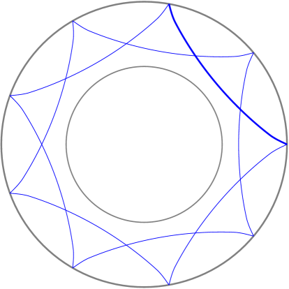
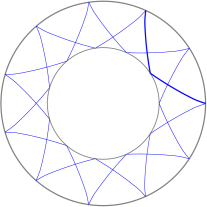
Figure 1. The first figure shows a closed orbit whose period is in $\operatorname{lsp}(c)$ and $\operatorname{lsp}^{\prime}(c)$. The second figure shows a closed orbit whose period is in $\operatorname{lsp}^{\prime}(c)$, but not in $\operatorname{lsp}(c)$.

We denote the Neumann spectrum of the Laplace–Beltrami operator in three dimensions, $\Delta_{c}=c^{3}\nabla\cdot c^{-1}\nabla$, on $M$ by $\operatorname{spec}(c)$, where we impose Neumann-type boundary conditions on both the inner and outer boundary. The spectrum $\operatorname{spec}(c)$ includes multiplicity, not just the set spectrum.

Some earlier results in tensor tomography the methods of which are related to ours may be found in [14, 15, 16, 17]. We are not aware of prior spectral rigidity results for manifolds with boundary. Two of the main theorems we prove on spectral rigidity are the following:

Theorem 1.1.

Let $B=\bar{B}(0,1)\setminus\bar{B}(0,R)\subset{\mathbb{R}}^{n}$, $n\geq 2$ and $R\geq 0$, be an annulus (or a ball if $R=0$). Fix $\varepsilon>0$ and let $c_{\tau}$, $\tau\in(-\varepsilon,\varepsilon)$, be a $C^{1,1}$ function $[R,1]\to(0,\infty)$ satisfying the Herglotz condition and the countable conjugacy condition and depending $C^{1}$-smoothly on the parameter $\tau$. If $R=0$, we assume $c_{\tau}^{\prime}(0)=0$. If $\operatorname{lsp}(c_{\tau})=\operatorname{lsp}(c_{0})$ for all $\tau\in(-\varepsilon,\varepsilon)$, then $c_{\tau}=c_{0}$ for all $\tau\in(-\varepsilon,\varepsilon)$.

The result holds true also for the length spectrum $\operatorname{lsp}^{\prime}(c)$ including reflections at the inner boundary, provided that $R>0$.

Theorem 1.2.

Let $B=\bar{B}(0,1)\setminus\bar{B}(0,R)\subset{\mathbb{R}}^{3}$, $R\geq 0$, be an annulus (or a ball if $R=0$). Fix $\varepsilon>0$ and let $c_{\tau}$, $\tau\in(-\varepsilon,\varepsilon)$, be a $C^{\infty}$ function $[R,1]\to(0,\infty)$ satisfying the Herglotz condition and the countable conjugacy condition and depending $C^{1}$-smoothly on the parameter $\tau$. Assume also that the length spectrum is non-degenerate in the sense that if two periodic broken rays have the same primitive period, then they differ by a rotation. If $R=0$, we assume that all odd order derivatives of $c_{\tau}$ vanish at $0$. If $\operatorname{spec}(c_{\tau})=\operatorname{spec}(c_{0})$ for all $\tau\in(-\varepsilon,\varepsilon)$, then $c_{\tau}=c_{0}$ for all $\tau\in(-\varepsilon,\varepsilon)$.

Theorem 1.1 is restated as theorems 4.6 (for $\operatorname{lsp}(c)$) and 4.7 (for $\operatorname{lsp}^{\prime}(c)$). We also prove an analogous theorem for the union of various spectra of this kind (theorem 4.8). We note that the dimension is irrelevant for the length spectral rigidity results; if the sound speed is fixed, the length spectrum is independent of dimension.

Using proposition C.1, we find the following corollaries:

Corollary 1.3.

Let $B=\bar{B}(0,1)\setminus\bar{B}(0,R)\subset{\mathbb{R}}^{n}$, $n\geq 2$ and $R\geq 0$, be an annulus (or a ball if $R=0$). Fix $\varepsilon>0$ and let $g_{\tau}$, $\tau\in(-\varepsilon,\varepsilon)$, be a $C^{1,1}$-regular non-trapping $SO(n)$-invariant Riemannian metric making the boundary strictly convex and satisfying the countable conjugacy condition and depending $C^{1}$-smoothly on the parameter $\tau$. If $\operatorname{lsp}(g_{\tau})=\operatorname{lsp}(g_{0})$ for all $\tau\in(-\varepsilon,\varepsilon)$, then there are rotation equivariant diffeomorphisms $\psi_{\tau}\colon B\to B$ so that $\psi^{*}_{\tau}g_{\tau}=g_{0}$ for all $\tau\in(-\varepsilon,\varepsilon)$.

In dimension $n\geq 3$ all rotation equivariant diffeomorphisms (diffeomorphisms commuting with the action of $SO(n)$) are radial. In dimension $n=2$ the diffeomorphisms are also radial if the metrics are assumed to be $O(2)$-invariant.

Corollary 1.4.

Let $B=\bar{B}(0,1)\setminus\bar{B}(0,R)\subset{\mathbb{R}}^{3}$, and $R\geq 0$, be an annulus (or a ball if $R=0$). Fix $\varepsilon>0$ and let $g_{\tau}$, $\tau\in(-\varepsilon,\varepsilon)$, be a $C^{\infty}$-regular non-trapping rotation invariant Riemannian metric making the boundary strictly convex and satisfying the countable conjugacy condition and depending $C^{1}$-smoothly on the parameter $\tau$. Assume also that the length spectrum is non-degenerate up to rotations. If $\operatorname{spec}(g_{\tau})=\operatorname{spec}(g_{0})$ for all $\tau\in(-\varepsilon,\varepsilon)$, then there are radial diffeomorphisms $\psi_{\tau}\colon B\to B$ so that $\psi^{*}_{\tau}g_{\tau}=g_{0}$ for all $\tau\in(-\varepsilon,\varepsilon)$.

Remark 1.5.

While our main results are stated for the Laplace–Beltrami operator, they are equally valid for the spectra associated to the toroidal modes (see [6, chapter 8.6] for a precise definition) of an elastic operator. In section 2, we point out that the length spectrum may be recovered from either the spectrum of the Laplace–Beltrami operator or the toroidal mode eigenfrequencies so the results above hold when one has the spectrum associated to toroidal modes. In fact, our trace formula (proposition 2.2) to recover the length spectrum from the spectrum is done for the more general toroidal modes and frequencies. Nevertheless, we show how our proof and result holds for the Laplace–Beltrami operator as well. We note that the spectrum of the Laplace–Beltrami operator depends on dimension.

The proofs of these theorems require three key ingredients which we elaborate in the next subsection:

1. A trace formula relating the Neumann spectrum of the Laplacian to the length spectrum. Thus, we will only need to prove length spectral rigidity since spectral rigidity (theorem 1.2) follows from the trace formula.

2. Sufficiently many periodic broken rays are stable under geometry-preserving perturbations of the metric and the derivative of the length of such broken rays is the periodic broken ray transform of the variation of the metric.

3. The periodic broken ray transform uniquely determines a radial function.

Outline of the proof

The breakup of the paper is as follows. In section 2, we discuss the relevant partial differential operators and their eigenfunctions. We also discuss geodesics in spherical symmetry and state the trace formula that we will prove (see proposition 2.2). Section 3 will be devoted to a proof of the trace formula. It will be necessary to use several transforms and the Debye expansion (see Appendix A) to convert the Green’s function for the wave propagator written in terms of eigenfunctions to the dynamical Fourier integral operator (FIO) representation analogous to the one in [8] and [10]. Along the way, the connection from eigenfunction to geodesics becomes rather explicit. To reinforce this point, in section 3.3 we revisit the wave propagator constructed in [10] and show how all our explicit calculations relate to the abstract, geometric construction in that paper. Finally, a standard application of the method of steepest descent and stationary phase provides the leading order asymptotics for the trace.

After proving the trace formula, we prove the rigidity of the length spectrum in section 4. Together with the trace formula this implies the rigidity of the Neumann spectrum of the Laplace–Beltrami operator. We have a family of radially symmetric wave speeds $c_{\tau}$ parameterized by $\tau\in(-\varepsilon,\varepsilon)$. For any periodic broken ray that is locally stable under the family of deformations, the derivative of its length is the integral of the metric variation over the periodic broken ray. In the case of closed manifolds and periodic geodesics this is well known, and in the case of non-periodic broken rays this was observed in [12]. Since the length spectrum is independent of the parameter $\tau$, these derivatives vanish. The countable conjugacy condition (definition 4.1) guarantees that sufficiently many periodic broken rays are stable, so that we may conclude that the periodic broken ray transform of the function $\left.\frac{\mathrm{d}}{\mathrm{d}\tau}c_{\tau}^{-2}\right|_{\tau=0}$ vanishes. It then follows from recent results of periodic broken ray tomography on spherically symmetric manifolds [7] that the function in question has to vanish. Since the function is radial, this can be seen as an injectivity result for an Abel-type integral transform. Consequently $c_{\tau}$ is independent of $\tau$ and the rigidity of the length spectrum and thus the spectrum follows.

Acknowledgements

M.V.d.H. gratefully acknowledges support from the Simons Foundation under the MATH + X program and the National Science Foundation under grant DMS-1559587. J.I. was supported by the Academy of Finland (decision 295853), and he is grateful for hospitality and support offered by Rice University during visits. V.K. thanks the Simons Foundation for financial support. We would also like to thank Gunther Uhlmann for helpful discussions and providing us useful references.

2. Geodesics and Eigenfunctions

In this section, we describe the relevant partial differential operators, associated eigenfunctions, and the connection between toroidal modes and the spectrum of the Laplace–Beltrami operator. We state our trace formula (proposition 2.2) along with an important remark related to the Laplace–Beltrami operator described in the introduction. First, let us provide a preliminary discussion of geodesics in spherically symmetric manifolds.

2.1. Geodesics in a spherically symmetric model

For the moment, we suppose that $n=2$ and equip the annulus $M=\bar{B}(0,1)\setminus\bar{B}(0,R)$ with spherical coordinates. For a maximal geodesic we define its radius as its Euclidean distance to the origin. We let $\gamma(r)$ be the maximal geodesic of radius $r$ which has its tip (the closest point to the origin) at the angular position $\theta=0$.

For $r_{0}\in(R,1)$, the geodesic $\gamma(r_{0})$ can be parametrized as

(2.1) $$[-L(r_{0}),L(r_{0})]\ni t\mapsto(r(t),\theta(t))$$

so that $r(0)=r_{0}$ and $\theta(0)=0$. Here $L(r_{0})>0$ is the half length of the geodesic. Using the conserved quantities $c(r(t))^{-2}[r^{\prime}(t)^{2}+r(t)^{2}\theta^{\prime}(t)^{2}]=1$ (squared speed) and $p=p_{\gamma}\coloneqq c(r(t))^{-2}r(t)^{2}\theta^{\prime}(t)=r_{0}/c(r_{0})$ (angular momentum) one can find the functions $r(t)$ and $\theta(t)$ explicitly.

Using these conserved quantities it is straightforward to show that

(2.2) $$L(r)=\int_{r}^{1}\frac{1}{c(r^{\prime})}\left(1-\left(\frac{rc(r^{\prime})}{r^{\prime}c(r)}\right)^{2}\right)^{-1/2}\mathrm{d}r^{\prime}=\int_{r}^{1}\frac{1}{c(r^{\prime})^{2}\beta(r^{\prime};p)}\mathrm{d}r^{\prime},$$

where $\beta(r;p)\coloneqq\sqrt{c^{-2}(r)-r^{-2}p^{2}}$. We introduce the quantity $\beta$ because it will appear naturally in the asymptotic approximations of eigenfunctions in section 3 and its relation to geodesics will now be clear.

We denote $\alpha(r)\coloneqq\theta(L(r))$, where $\theta$ is the angular coordinate (taking values in ${\mathbb{R}}$) of the geodesic $\gamma(r)$. That is, $2\alpha(r)$ is the angular distance of the endpoints of $\gamma(r)$. It may happen that $\alpha(r)>\pi$ if the geodesic winds around the origin several times. Using the invariants given above, one can also find an explicit formula for $\alpha(r)$:

(2.3) $$\alpha(r)=\int_{r}^{1}\frac{rc(r^{\prime})}{c(r)(r^{\prime})^{2}}\left(1-\left(\frac{rc(r^{\prime})}{r^{\prime}c(r)}\right)^{2}\right)^{-1/2}\mathrm{d}r^{\prime}=\int_{r}^{1}\frac{p}{(r^{\prime})^{2}\beta(r^{\prime};p)}\mathrm{d}r^{\prime}.$$

We will use the following lemma without mention whenever we need regularity of these functions.

Lemma 2.1.

When $c$ is $C^{1,1}$ and satisfies the Herglotz condition, then the functions $\alpha$ and $L$ are $C^{1}$ on $(R,1)$.

Proof.

This follows from equations (35), (67), and (68) and proposition 15 in [7]. ∎

2.2. Toroidal modes, eigenfrequencies, and traces

We now use spherical coordinates $(r,\theta,\psi)$. Toroidal modes are precisely the eigenfunctions of the isotropic elastic operator that are sensitive to only the shear wave speed. We forgo writing down the full elastic equation, and merely write down these special eigenfunctions connected to the shear wave speed (full details with the elastic operator may be found in [6, chapter 8.6]). Analytically, these eigenfunctions admit a separation in radial functions and real-valued spherical harmonics, that is,

(2.4) $$u={}_{n}\mathbf{D}_{l}Y^{m}_{l},$$

where

(2.5) $$\mathbf{D}=U(r)\ (-k^{-1})[-\widehat{\theta}(\sin\theta)^{-1}\partial_{\psi}+\widehat{\psi}\partial_{\theta}],$$

in which $k=\sqrt{l(l+1)}$ (instead of the asymptotic Jeans relation, $k=l+\tfrac{1}{2}$) and $U$ represents a radial function (${}_{n}U_{l}$). In the further analysis, we ignore the curl (which signifies a polarization); that is, we think of ${}_{n}\mathbf{D}_{l}$ as the multiplication with ${}_{n}U_{l}(-k^{-1})$. In the above, $Y^{m}_{l}$ are spherical harmonics, defined by

$$Y^{m}_{l}(\theta,\psi)=\left\{\begin{array}[]{rcl}\sqrt{2}X^{\left\lvert m\right\rvert}_{l}(\theta)\cos(m\psi)&\text{if}&-l\leq m<0,\\ X^{0}_{l}(\theta)&\text{if}&m=0,\\ \sqrt{2}X^{m}_{l}(\theta)\sin(m\psi)&\text{if}&0<m\leq l,\end{array}\right.$$

where

$$X^{m}_{l}(\theta)=(-)^{m}\sqrt{\frac{2l+1}{4\pi}}\sqrt{\frac{(l-m)!}{(l+m)!}}P^{m}_{l}(\cos\theta),$$

in which

$$P^{m}_{l}(\cos(\theta))=(-)^{m}\frac{1}{2^{l}l!}(\sin\theta)^{m}\left(\frac{1}{\sin\theta}\frac{\mathrm{d}}{\mathrm{d}\theta}\right)^{l+m}(\sin\theta)^{2l}.$$

The function, $U$ (a component of displacement), satisfies the equation

(2.6) $$[-r^{-2}\partial_{r}\ r^{2}\mu\partial_{r}+r^{-2}\partial_{r}\ \mu r-r^{-1}\mu\partial_{r}+r^{-2}(-1+k^{2})\mu]\,U-\omega^{2}\rho U=0,$$

where $\mu=\mu(r)$ is a Lamé parameter and $\rho=\rho(r)$ is the density, both of which are smooth. Also, $\omega={}_{n}\omega_{l}$ denotes the associated eigenvalue. Here, $l$ is referred to as the angular order and $m$ as the azimuthal order.

The traction is given by

(2.7) $$T(U)=\mathcal{N}U,\qquad\mathcal{N}=\mu\partial_{r}-r^{-1}\mu$$

which vanishes at the boundaries (Neumann condition). The radial equations do not depend on $m$ and, hence, every eigenfrequency is degenerate with an associated $(2l+1)$-dimensional eigenspace spanned by

$$\{Y^{-l}_{l},\ldots,Y^{l}_{l}\}.$$

We use spherical coordinates $(r_{0},\theta_{0},\psi_{0})$ for the location, $x_{0}$, of a source, and introduce the shorthand notation $({}_{n}\mathbf{D}_{l})_{0}$ for the operator expressed in coordinates $(r_{0},\theta_{0},\psi_{0})$. We now write the (toroidal contributions to the) fundamental solution as a normal mode summation

(2.8) $$G(x,x_{0},t)=\operatorname{Re}\ \sum_{l=0}^{\infty}\sum_{n=0}^{\infty}\ {}_{n}\mathbf{D}_{l}({}_{n}\mathbf{D}_{l})_{0}\ \sum_{m=-l}^{l}Y^{m}_{l}(\theta,\psi)Y^{m}_{l}(\theta_{0},\psi_{0})\ \frac{e^{\operatorname{i}{}_{n}\omega_{l}t}}{\operatorname{i}{}_{n}\omega_{l}}.$$

On the diagonal, $(r,\theta,\psi)=(r_{0},\theta_{0},\psi_{0})$ and, hence, $\Theta=0$. Here $\Theta$ is the angular epicentral distance, cf. (3.2). We observe the following reductions in the evaluation of the trace of (2.8):

• The functions $U(r)$ are normalized, so that

  (2.9) $$\int_{R}^{1}U(r)^{2}\rho(r)r^{2}\operatorname{d}\!r=1.$$

  Meanwhile, the spherical harmonic terms satisfy

  (2.10) $$\sum_{m=-l}^{l}\iint Y^{m}_{l}(\theta,\psi)^{2}\sin\theta\operatorname{d}\!\theta\operatorname{d}\!\psi=2l+1$$

  (counting the degeneracies of eigenfrequencies).

• If we were to include the curl in our analyis (generating vector spherical harmonics), taking the trace of the matrix on the diagonal yields

  (2.11) $$\sum_{m=-l}^{l}\iint(-k^{-2})\left\lvert[-\widehat{\theta}(\sin\theta)^{-1}\partial_{\psi}+\widehat{\psi}\partial_{\theta}]Y^{m}_{l}(\theta,\psi)\right\rvert^{2}\sin\theta\operatorname{d}\!\theta\operatorname{d}\!\psi=2l+1.$$

From the reductions above, we obtain

(2.12) $$\int_{M}G(x,x,t)\,\rho(x)\operatorname{d}\!x=\sum_{l=0}^{\infty}\sum_{n=0}^{\infty}\ (2l+1)\operatorname{Re}\left\{\frac{e^{\operatorname{i}{}_{n}\omega_{l}t}}{\operatorname{i}{}_{n}\omega_{l}}\right\}$$

or

(2.13) $$\operatorname{Tr}(\partial_{t}G)(t)=\int_{M}\partial_{t}G(x,x,t)\,\rho(x)\operatorname{d}\!x=\sum_{l=0}^{\infty}\sum_{n=0}^{\infty}\ (2l+1)\operatorname{Re}\left\{e^{\operatorname{i}{}_{n}\omega_{l}t}\right\}.$$

We now write

$${}_{n}f_{l}(t)=\operatorname{Re}\left\{\frac{e^{\operatorname{i}{}_{n}\omega_{l}t}}{\operatorname{i}{}_{n}\omega_{l}}\right\}$$

which is the inverse Fourier transform of

(2.14) $${}_{n}\hat{f}_{l}(\omega)=\frac{1}{2\operatorname{i}{}_{n}\omega_{l}}\left[\mbox{\rule{0.0pt}{14.22636pt}}\right.\pi\delta(\omega-{}_{n}\omega_{l})-\pi\delta(\omega+{}_{n}\omega_{l})\left.\mbox{\rule{0.0pt}{14.22636pt}}\right].$$

Moreover, taking the Laplace–Fourier transform yields

(2.15) $$\int_{0}^{\infty}{}_{n}f_{l}(t)e^{-\operatorname{i}\omega t}\,\operatorname{d}\!t=\frac{1}{2\operatorname{i}{}_{n}\omega_{l}}\left[\mbox{\rule{0.0pt}{14.22636pt}}\right.\frac{\operatorname{i}}{-(\omega-{}_{n}\omega_{l})+\operatorname{i}0}-\frac{\operatorname{i}}{-(\omega+{}_{n}\omega_{l})+\operatorname{i}0}\left.\mbox{\rule{0.0pt}{14.22636pt}}\right].$$

This confirms that the trace is equal to the inverse Fourier transform of

$$\sum_{l=0}^{\infty}(2l+1)\sum_{n=0}^{\infty}\frac{1}{2\operatorname{i}{}_{n}\omega_{l}}\left[\mbox{\rule{0.0pt}{14.22636pt}}\right.\pi\delta(\omega-{}_{n}\omega_{l})-\pi\delta(\omega+{}_{n}\omega_{l})\left.\mbox{\rule{0.0pt}{14.22636pt}}\right].$$

In the next subsection, we explain how the toroidal eigenfrequencies $\{{}_{n}\omega_{l}\}_{n,l}$ relate to the Neumann spectrum of the Laplace–Beltrami operator described in the introduction. We also show why all our results and proofs in connection to the trace formula (proposition 2.2) hold for this spectrum as well.

2.3. Connection between toroidal eigenfrequencies, spectrum of the Laplace–Beltrami operator, and the Schrödinger equation

We relate the spectrum of a scalar Laplacian, the eigenvalues associated to the vector valued toroidal modes, and the trace distribution $\sum_{l=0}^{\infty}\sum_{n=0}^{\infty}\ (2l+1)\cos(t{}_{n}\omega_{l})$.

We note that (2.6) and (2.7) for $U$ ensure that $v=UY^{m}_{l}$ satisfies

(2.16) $$Pv\coloneqq\rho^{-1}(-\nabla\cdot\mu\nabla+P_{0})v=\omega^{2}v,\qquad\mathcal{N}v=0\text{ on }\partial M$$

where $P_{0}=r^{-1}(\partial_{r}\mu)$ is a $0$th order operator and $\omega^{2}$ is a particular eigenvalue. Hence $UY^{m}_{l}$ are scalar eigenfunctions for the self-adjoint (with respect to the measure $\rho\operatorname{d}\!x$) scalar operator $P$ with Neumann boundary conditions (on both boundaries) expressed in terms of $\mathcal{N}$.

The above argument shows that we may view the toroidal spectrum $\{{}_{n}\omega^{2}_{l}\}_{n,l}$ as also the collection of eigenvalues $\lambda$ for the boundary problem on scalar functions (2.16). Thus (2.13) can be written in the form

(2.17) $$\operatorname{Tr}\,(\partial_{t}G)=\sum_{\lambda\in\operatorname{spec}(P)}\cos(t\sqrt{\lambda}),$$

where the last sum is taken with multiplicities for the eigenvalues. (While $G$ is a vector valued distribution, the asymptotic trace formula we obtain is for $\operatorname{Tr}(\partial_{t}G)$, which is equal to $\sum_{\lambda\in\operatorname{spec}(P)}\cos(t\sqrt{\lambda})$ by the normalizations we have chosen.) Up to principal symbols, $P$ coincides with the $\Delta_{c}=c^{3}\nabla\cdot c^{-1}\nabla$ upon identifying $c^{2}$ with $\rho^{-1}\mu$. This means that the length spectra of $P$ and $\Delta_{c}$ will be the same even though they have differing subprincipal symbols and spectra. Thus, the trace formula which will appear to have a unified form, connects two different spectra to a common length spectrum and the proof is identical for both.

For concreteness, we recall [10, theorem 1]. Suppose that $\lambda_{1}\leq\lambda_{2}\leq\dots\to\infty$ denote the Neumann spectrum of the Laplace–Beltrami operator $\Delta_{g}$. We form the distribution

(2.18) $$\sum_{\lambda\in\operatorname{spec}(\Delta_{g})}\cos(t\sqrt{\lambda}).$$

Under certain geometric conditions (where there is no symmetry) for a simpler manifold described there, the authors prove the following: Let $T$ be the singular support of (2.18) and the only closed geodesics, $\gamma$, of period $T$ satisfy certain geometric conditions and have Maslov indices $\sigma_{\gamma}$. Then for $t$ near $T$, (2.18) is equal to the real part of

(2.19) $$\sum_{T_{\gamma}=T}\operatorname{i}^{\sigma_{\gamma}}\frac{T^{\sharp}_{\gamma}}{(|I-P_{\gamma}|)^{1/2}}(t-T+0\operatorname{i})^{-1}+L^{1}_{loc},$$

where $T^{\sharp}$ is the primitive period and $P_{\gamma}$ is a certain Poincaré map described there. Our results will settle the question of whether there is a formula analogous to (2.19) (same as [10, (1.3)]) for the distributions $\sum_{\lambda\in\operatorname{spec}(P)}\cos(t\sqrt{\lambda})$ and $\sum_{\lambda\in\operatorname{spec}(c)}\cos(t\sqrt{\lambda})$ in our spherically symmetric manifold with boundary, encompassing a ball and an annulus.

We will prove a trace formula using a WKB expansion of eigenfunctions. To this end, it is convenient to establish a connection with the Schrödinger equation. Indeed, we present an asymptotic transformation finding this connection. In boundary normal coordinates $(r,\theta)$ (which are spherical coordinates in dimension three by treating $\theta$ as coordinates on the $2$-sphere),

(2.20) $$P=\rho^{-1}(-r^{-2}\partial_{r}r^{2}\mu\partial_{r}-\mu r^{-2}\Delta_{\theta}+P_{0}),$$

where $\Delta_{\theta}$ is the Laplacian on the $2$-sphere. We write $\lambda=\omega^{2}$ as before and rewrite the second-order equation (2.16) in the form

(2.23) $$Y =\left(\begin{array}[]{l}rv\\ r\mathcal{N}v\end{array}\right),$$

(2.24) $$\partial_{r}Y =A(r,\omega)Y,$$

where

$$A_{11} =2r^{-1},$$

$$A_{21} =(-\Delta_{\theta}-2)r^{-2}\mu-\omega^{2}\rho,$$

$$A_{12} =\mu^{-1},$$

$$A_{22} =-2r^{-1},$$

satisfying

$$JA=-A^{*}J\quad\text{with}\quad J=\left(\begin{array}[]{rr}0&1\\ -1&0\end{array}\right),\quad J^{2}=-I.\qquad$$

The Neumann condition is applied at $r=1$ and at $r=R$. In preparation of the asymptotic analysis we will instead invoke the transformation using the same notation (by abuse of notation, cf. (2.23))

(2.25) $$Y=\left(\begin{array}[]{l}rv\\ \omega^{-1}r\mathcal{N}v\end{array}\right).$$

With this definition, the matrix $A$ in (2.24) admits the expansion

(2.26) $$A(r,\omega)=\omega\,[A_{0}(r)+\omega^{-1}A_{1}(r)+\omega^{-2}A_{2}(r)],$$

$$A_{0}(r)=\begin{pmatrix}0&\mu^{-1}\\ -\rho-r^{-2}\omega^{-2}\mu\Delta_{\theta}&0\end{pmatrix},\quad A_{1}(r)=\begin{pmatrix}2r^{-1}&0\\ 0&-2r^{-1}\end{pmatrix},$$

$$A_{2}(r)=\begin{pmatrix}0&0\\ -2r^{-2}\mu&0\end{pmatrix},$$

viewing $\omega$ as a large parameter. A similarity transform gives

(2.27) $$A_{0}R=R\Lambda,\qquad\Lambda(r)=\begin{pmatrix}0&1\\ -\tilde{\beta}^{2}&0\end{pmatrix},\ \ R(r)=\begin{pmatrix}\mu^{-1/2}&0\\ 0&\mu^{1/2}\end{pmatrix},$$

where we have defined

(2.28) $$\tilde{\beta}^{2}=\rho(r)\mu(r)^{-1}+\omega^{-2}r^{-2}\Delta_{\theta}.$$

We then seek an asymptotic transformation $L$ and $W$

$$Y=LW\quad\text{with}\quad L(r,\omega)=\sum_{j\geq 0}L_{j}(r)\omega^{-j},$$

so that the original matrix system implies

(2.29) $$\partial_{r}W=\omega\Lambda(r)W.$$

Substitution and equating terms with equal powers of $\omega^{-1}$ gives

(2.30) $$A_{0}L_{0}-L_{0}\Lambda = 0,$$

(2.31) $$A_{0}L_{1}-L_{1}\Lambda = \partial_{r}L_{0}-A_{1}L_{0},$$

and so on. We find a simple solution

(2.32) $$L_{0}=r^{-1}R(r).$$

Then

(2.33) $$\begin{split}L_{0}W&=\left(\begin{array}[]{l}\mu^{-1/2}w\\ \omega^{-1}\mu^{1/2}\partial_{r}w\end{array}\right),\\ rv&=\mu^{-1/2}w,\\ r\mathcal{N}v&=\mu^{1/2}\partial_{r}w,\\ W_{1}&=rw,\\ W_{2}&=\omega^{-1}r\partial_{r}w.\end{split}$$

Here, $w$ satisfies the equation

(2.34) $$(\partial_{r}^{2}+r^{-2}\Delta_{\theta}+\omega^{2}\rho\mu^{-1})w=0,\qquad\partial_{r}w=0\ \text{ on }\ \partial M.$$

If $y(\theta)$ is an eigenfunction of $\Delta_{\theta}$ with eigenvalue $-k^{2}$ and $V=V(r)$ is radial function, we choose $w=w_{k}=V(r)y(\theta)$ so that $V(r)$ must now satisfy

(2.35) $$\partial_{r}^{2}V+\omega^{2}\beta^{2}V=0,\quad\partial_{r}V=0\ \text{ on }\ \partial M,$$

where $\beta=\rho(r)\mu(r)^{-1}-\omega^{-2}r^{-2}k^{2}$, generating two linearly independent solutions. The WKB asymptotic solution to this PDE with Neumann boundary conditions will precisely give us the leading order asymptotics for the trace formula, and is all that is needed. We note that

$$rU=\mu^{-1/2}V\ \text{ and }\ rT(r)=\mu^{1/2}\partial_{r}V.$$

For the boundary condition, we note that we would end up with the same partial differential equation with different boundary conditions for $V$ in the previous section if we had used the boundary condition $\partial_{r}u=0\text{ on }\partial M$. Indeed, one would merely choose $\mathcal{N}u=\mu\partial_{r}u$ instead without the $0$’th order term. However, the boundary condition for $V$ would be of the form

$$\partial_{r}V=K(r)V\quad\ \text{ on }\ \partial M$$

with $K$ signifying a smooth radial function. Nevertheless, the leading order (in $\omega$) asymptotic behavior for $V$ stays the same despite the $K$ term as clearly seen in the calculation of section 3.1.1. Thus, our analysis applies with no change using the standard Neumann boundary conditions. This should come as no surprise since in [10], the $0$’th order term in the Neumann condition played no role in the leading asymptotic analysis of their trace formula. Only if one desires the lower-order terms in the trace formula would it play a role.

2.4. Poincaré maps and the trace formula

Here, we describe the relevant Poincaré map that will appear in the trace formula and state the trace formula that we will prove. Let $\mathbb{R}\ni t\to\gamma(t)$ be a periodic broken bicharacteristic in $S^{*}M$ of period $T>0$ (see [10] for the relevant definitions). It is associated to the metric $c^{-2}(\left\lvert x\right\rvert)e$, where $c$ is a smooth radial function, $e$ is the Euclidean metric, and $\gamma$ undergoes reflections in $\partial S^{*}M$ according to Snell’s law. We also denote by $\Phi^{T}\colon S^{*}M\to S^{*}M$ the broken bicharacteristic flow of $T$ units of time as described in [10]. Its fixed point set is given by

$$C_{T}\coloneqq\{\eta\in S^{*}M;\Phi^{T}(\eta)=\eta\}$$

and without loss of generality, we assume that $C_{T}$ is connected, for otherwise, we would look at a connected component instead. We impose the clean intersection hypothesis appearing in [8, 10] so that $C_{T}$ is a submanifold for any $T$ and $T_{m}C_{T}=\ker(\operatorname{Id}-\mathrm{d}\Phi^{T}(m))$ at each point $m\in C_{T}$. This holds for all periodic orbits if and only if $c$ satisfies the periodic conjugacy condition (definition 4.2) which requires that the endpoints of a single maximal geodesic segment of a periodic broken ray are never conjugate; see remark 4.3.

By construction, the image of $\gamma$ belongs to $C_{T}$. There is an obvious symplectic group action of $SO(3)$ on $T^{*}M$ under which the Hamiltonian $\frac{1}{2}c^{2}\left\lvert\xi\right\rvert^{2}$ is invariant; here, $\xi$ denotes the dual variable to $x$. Thus, for each $g\in SO(3)$, the set $g\cdot\operatorname{Im}(\gamma)$ given by the group action also belongs to $C_{T}$. Assuming that $c$ has no other symmetries (follows from the Herglotz condition) and the periodic conjugacy condition, all elements of $C_{T}$ are obtained this way. This is because a periodic orbit will either fail to be periodic or not have period $T$ after a small perturbation of the angular momentum $p$; hence, $p$ remains constant on $C_{T}$. Thus, $C_{T}$ may be parameterized by $\mathbb{R}_{t}\times SO(3)$, revealing that under the Herglotz and periodic conjugacy conditions

$$\dim(C_{T})=4.$$

The Herglotz condition ensures that the group action never coincides with the geodesic flow; without it, the dimension could quite possibly be smaller. Hence, $T_{m}S^{*}M/T_{m}C_{T}$ is only one-dimensional and we obtain an induced map on the quotient space,

$$I-\mathrm{d}\Phi^{T}\colon T_{m}S^{*}M/T_{m}C_{T}\to T_{m}S^{*}M/T_{m}C_{T}.$$

We denote the equivalence class of all closed orbits of period $T$ related to $\gamma$ by an element of $SO(3)$ or by a time reversal of $\gamma$ by $[\gamma]$. We write the above map as $I-P_{[\gamma]}$ and refer to $P_{[\gamma]}$ as the Poincaré map associated to the equivalence class of $\gamma$. Now, $I-P_{[\gamma]}$ will end up being an isomorphism, whose determinant at each point $m\in C_{T}$ will stay invariant. Hence, the quantity $\left\lvert I-P_{[\gamma]}\right\rvert^{-1}\coloneqq\left\lvert\operatorname{det}(I-P_{[\gamma]})\right\rvert^{-1}$ is well defined as a single number associated to $[\gamma]$.

In the above, $\gamma$ may be multiple revolutions of another closed orbit of minimal period called the primitive orbit associated to $\gamma$, which has a primitive period denoted $T^{\sharp}$. Note that $T$ will merely be a positive integer multiple of $T^{\sharp}$. In spherical symmetry, $\gamma$ is confined to a disk and it must be a concatenation of geodesic segments that travel from the outer boundary $r=1$ to either the reflection point $r=R$ or the turning point $r=R^{\star}$ (see section 4 for details). We let $N_{\gamma}$ denote the number of these segments comprising the primitive orbit associate to $\gamma$.

We now state our proposition pertaining to the trace formula.

Proposition 2.2.

Suppose the radial wave speed $c$ satisfies the Herglotz condition and the periodic conjugacy condition (definition 4.2). Assume additionally that the length spectrum is non-degenerate in the sense that any two periodic broken rays of the same length are rotations of each other.

The distribution $(\operatorname{Tr}\,(\partial_{t}G))(t)=\sum_{n,l}(2l+1)\cos(t{}_{n}\omega_{l})$ is singular precisely at the length spectrum. Suppose $T\in\operatorname{singsupp}(\operatorname{Tr}(\partial_{t}G))$ and let $d$ be the dimension of the fixed point set for $\Phi^{T}$. Suppose that $\gamma$ is one of the broken periodic orbits of period $T$. Then $d=4$ and for $t$ near $T$, the contribution of $[\gamma]$ to the leading singularity of $(\operatorname{Tr}(\partial_{t}G))(t)$ is the real part of

$$(t-T+\operatorname{i}0)^{-(d+1)/2}\left(\frac{1}{2\pi\operatorname{i}}\right)^{(d-1)/2}\operatorname{i}^{\sigma_{\gamma}}\left\lvert I-P_{[\gamma]}\right\rvert^{-1/2}\frac{T^{\sharp}_{\gamma}}{2\pi N_{\gamma}}c_{d}\left\lvert SO(3)\right\rvert,$$

where

1. $\sigma_{\gamma}$ is the KMAH index associated to $\gamma$ defined in [10];

2. $c_{d}$ is a constant depending only on $d$;

3. $\left\lvert SO(3)\right\rvert$ is the volume of the compact Lie group $SO(3)$ under the Haar measure.

In appendix B we identify this trace formula in the framework of manifolds with symmetries given by a compact Lie group. In appendix D we discuss some edge cases that justify our geometric assumptions.

Remark 2.3.

This trace formula is in fact a more general statement than that for the Neumann Laplace–Beltrami operator, which is just a special case of the above proposition.

Remark 2.4.

The periodic conjugacy condition and non-degeneracy of the length spectrum are needed to prove that the singular support of the trace is precisely the length spectrum. However, they are not necessary for spectral rigidity or proving that the spectrum determines the length spectrum.

For unique determination of the length spectrum, it is enough that the primitive length spectrum (excluding all but primitive orbits) is non-degenerate. Given the singularity at $T^{\sharp}$, we know what the singularities at $2T^{\sharp},3T^{\sharp},\dots$ will be. If they are not as expected, then another broken ray must contribute a singularity at the same place, and we have found the next primitive length. This allows to recover the primitive length spectrum and therefore the whole length spectrum from the (shapes and locations of) singularities in the trace. But if two primitive lengths coincide, there is no way to distinguish the corresponding singularities.

If we drop the periodic conjugacy condition, then some periodic orbits may fail the clean intersection hypothesis. This allows us to recover only a part of the length spectrum from the singularities, but this part is enough. Such problematic periodic broken rays are ignored anyway in the proof of length spectral rigidity, since they might not be stable under deformations.

3. Proof of the Trace Formula (proposition 2.2)

In this section, we prove the trace formula in the form of proposition 2.2 for the annulus. The idea behind the proof is to construct rather explicitly a fundamental solution. First, we do some preliminary analysis to manipulate $G$ into the right form before taking its trace. Concretely, in subsection 3.1, we construct WKB eigenfunction solutions to get explicit formulas for the leading order asymptotics of the eigenfunctions. Afterwards, in subsection 3.2 we use the classical Poisson summation formula and the Debye expansion to write the leading order asymptotics for $G$ as a certain propagator, which relates the eigenfunctions to geodesics in the annulus. At that point, we use section 3.3 to show how all our constructions are quite natural and directly relate to the wave propagator appearing in [10]. Finally, we complete the proof in section 3.4 by taking traces and carrying out the method of steepest descent and stationary phase to obtain the desired asymptotic formula appearing in proposition 2.2.

In the further analysis, we employ the summation formula,

(3.1) $$\sum_{m=-l}^{l}Y^{m}_{l}(\theta,\psi)Y^{m}_{l}(\theta_{0},\psi_{0})=\frac{(2l+1)}{4\pi}\,P_{l}(\cos\Theta),$$

where the $P_{l}$ are the Legendre polynomials, with $P_{l}(1)=1$, and $\Theta$ signifies the angular epicentral distance,

(3.2) $$\cos\Theta\ =\ \cos\theta\,\cos\theta_{0}+\sin\theta\,\sin\theta_{0}\,\cos(\psi-\psi_{0}).$$

Remark 3.1.

We note that $\hat{G}$ is the kernel of the resolvent in the time-harmonic formulation. The normal mode summation becomes

(3.3) $$\hat{G}(x,x_{0},\omega)=\frac{1}{2\pi}\ \sum_{l=0}^{\infty}\sum_{n=0}^{\infty}\ (l+\tfrac{1}{2})\ {}_{n}\hat{f}_{l}(\omega)\ \underbrace{{}_{n}\mathbf{D}_{l}({}_{n}\mathbf{D}_{l})_{0}}_{\eqqcolon{}_{n}H_{l}}\ P_{l}(\cos\Theta),$$

explicitly showing the eigenfrequencies as simple poles (cf. (2.15)).

We abuse notation and denote

$${}_{n}H_{l}=k^{-2}U(r)U(r_{0})$$

in the formula for $G$ to not treat the curl operations at first. This will not cause a risk of confusion since we will specify the exact moment that we apply the curl operators, which will be just before taking the trace in subsection 3.4.

3.1. Asymptotic analysis of eigenfunctions

We describe the radial eigenfunctions and their asymptotic expansions for general $k\in\mathbb{R}$. We then introduce the dispersion relations, $\omega_{n}(k)$.

3.1.1. WKB eigenfunctions

Here, we consider asymptotic solutions, $V$, to (2.35). Depending on $p$, we distinguish the following regimes:

• Evanescent ($1/c(1)<p<\infty$). Here, $\beta^{2}(r)<0$, and the solution is always non-oscillatory, that is, evanescent. We do not obtain eigenfunctions.

• Diving ($R/c(R)<p<1/c(1))$: We summarize the WKB solution of (2.35) in the vicinity of a general turning point. A turning point, $r=R^{\star}$, is determined by

  $$\beta^{2}(R^{\star})=0.$$

  Near a turning point, $r\approx R^{\star}$, and

  $$\beta^{2}(r)\simeq\alpha_{0}(r-R^{\star}).$$

  Away from a turning point,

  $$\beta^{2}>0\text{ if $r\gg R^{\star}$},\quad\beta^{2}<0\text{ if $r\ll R^{\star}$}.$$

  Matching asymptotic solutions yields

  (3.4) $$B\begin{cases}\left\lvert\beta\right\rvert^{-1/2}\exp\left(-\omega\int_{r}^{R^{\star}}\left\lvert\beta\right\rvert\,\operatorname{d}\!r\right),&r\ll R^{\star}\\[5.0pt] 2\pi^{1/2}\alpha_{0}^{-1/6}\omega^{1/6}\mathrm{Ai}(-\omega^{2/3}\alpha_{0}^{1/3}(r-R^{\star})),&r\simeq R^{\star}\\[5.0pt] 2\beta^{-1/2}\cos\left(-\omega\int_{R^{\star}}^{r}\beta\,\operatorname{d}\!r-\pi/4\right),&r\gg R^{\star}.\end{cases}$$

  From these one can obtain a uniform expansion, that is, the Langer approximation

  (3.5) $$\begin{split}V(r,\omega;p)&=2\pi^{1/2}\chi^{1/6}(-\beta^{2})^{-1/4}\mathrm{Ai}(\chi^{2/3}(r)),\\ \chi(r)&=-(3/2)\omega\int_{R^{\star}}^{r}(-\beta^{2})^{1/2}\operatorname{d}\!r,\end{split}$$

  valid for $r\in[R,1]$. One obtains eigenfunctions corresponding with turning rays.

  Up to leading order, where $r\gg R^{\star}$,

  (3.6) $$V =2B\beta^{-1/2}\cos\left(\omega\int_{R^{\star}}^{r}\beta\,\operatorname{d}\!r^{\prime}-\pi/4\right),$$

  (3.7) $$\partial_{r}V =-2\omega B\beta^{-1/2}\sin\left(\omega\int_{R^{\star}}^{r}\beta\,\operatorname{d}\!r^{\prime}-\pi/4\right).$$

  Here, $B$ is obtained from the normalization (2.9), which requires the uniformly asymptotic solution over the entire interval $[R,1]$. Applying the Riemann–Lebesgue lemma, one obtains

  (3.8) $$\int_{R}^{1}U(r)^{2}\rho(r)r^{2}\operatorname{d}\!r\simeq 2B^{2}\int_{R^{\star}}^{1}\beta^{-1}c^{-2}\operatorname{d}\!r.$$

  Here, $\int_{R^{\star}}^{1}\beta^{-1}c^{-2}\operatorname{d}\!r$ can be identified with the half one-return travel time, $\tfrac{1}{2}T$, say.

• Reflecting ($0<p<R/c(R))$: The solutions are oscillatory in the entire interval $[R,1]$ ($\beta^{2}(r;p)>0$), correspond with reflecting rays, and are of the form

  (3.9) $$V =C\beta^{-1/2}\exp\left(\operatorname{i}\omega\int_{R}^{r}\beta\operatorname{d}\!r^{\prime}\right)+D\beta^{-1/2}\exp\left(-\operatorname{i}\omega\int_{R}^{r}\beta\operatorname{d}\!r^{\prime}\right),$$

  (3.10) $$\partial_{r}V =\operatorname{i}\omega C\beta^{1/2}\exp\left(\operatorname{i}\omega\int_{R}^{r}\beta\operatorname{d}\!r^{\prime}\right)-\operatorname{i}\omega D\beta^{1/2}\exp\left(-\operatorname{i}\omega\int_{R}^{r}\beta\operatorname{d}\!r^{\prime}\right).$$

  to leading order. Imposing the Neumann condition, $T(R)=0$, implies that $D=C$. The constant $C$ is obtained from the normalization (2.9) using the oscillatory solution over the entire interval $[R,1]$. Applying the Riemann–Lebesgue lemma yields

  (3.11) $$\int_{R}^{1}U(r)^{2}\rho(r)r^{2}\operatorname{d}\!r\simeq 2C^{2}\int_{R}^{1}\beta^{-1}c^{-2}\operatorname{d}\!r.$$

  Here, $\int_{R}^{1}\beta^{-1}c^{-2}\operatorname{d}\!r$ can be identified with the half one-return reflection travel time, $\tfrac{1}{2}T$, say.

3.1.2. Boundary condition and dispersion relations

We backsubstitute $p=\omega^{-1}k$ in $\beta$. Imposing the Neumann boundary condition yields:

• Diving ($R/c(R)<p<1/c(1))$:

  (3.12) $$\omega\int_{R^{\star}}^{1}\beta(r^{\prime};\omega^{-1}k)\,\operatorname{d}\!r^{\prime}=\left(n+\frac{5}{4}\right)\pi\quad\text{($n$ is the overtone index)}.$$

• Reflecting ($0<p<R/c(R)$):

  (3.13) $$\omega\int_{R}^{1}\beta(r^{\prime};\omega^{-1}k)\operatorname{d}\!r^{\prime}\ =\ (n+1)\pi\quad\text{($n$ is the overtone index)}.$$

All these (radial) quantization-type conditions yield solutions ${}_{n}\omega_{k}\eqqcolon\omega_{n}(k)$. Using the implicit function theorem, we introduce $k_{n}=k_{n}(\omega)$ as the solution of

$$\omega-\omega_{n}(k_{n})=0.$$

We revisit the general relation between phase and group velocities. We have

$$c_{n}(k)=\frac{\omega_{n}(k)}{k}$$

and

$$C_{n}=\frac{{\mathrm{d}}(c_{n}k)}{{\mathrm{d}}k}=c_{n}+k\,\frac{{\mathrm{d}}c_{n}}{{\mathrm{d}}k}.$$

The corresponding ray parameter is given by

(3.14) $$p=\frac{k}{\omega_{n}(k)}=\frac{1}{c_{n}(k)}.$$

3.2. Poisson’s summation formula

3.2.1. Analytic continuation

The Legendre equation is of second order and hence admits two linearly independent solutions: Legendre functions of the first and second kind, $P_{\lambda}$, $Q_{\lambda}$, with integral representations

(3.15) $$P_{\lambda}(z) =\frac{2}{\pi}\operatorname{Im}\int_{0}^{\infty}\left[z-\operatorname{i}\sqrt{1-z^{2}}\cosh(t)\right]^{-\lambda-1}\,\operatorname{d}\!t,$$

(3.16) $$Q_{\lambda}(z) =\phantom{\frac{2}{\pi}}\operatorname{Re}\int_{0}^{\infty}\left[z-\operatorname{i}\sqrt{1-z^{2}}\cosh(t)\right]^{-\lambda-1}\,\operatorname{d}\!t,$$

for $z\in[-1,1]$. These integral representations are valid for $\operatorname{\lambda}>-1$. Analytic continuation of the integral representation for $P_{\lambda}$, $Q_{\lambda}$ into the region $\operatorname{Re}\{\lambda\}\leq-1$ follows the relations

(3.17) $$P_{-\lambda-1} = P_{\lambda},$$

(3.18) $$Q_{-\lambda-1} = Q_{\lambda}-\pi\,\cot(\lambda\pi)\,P_{\lambda}.$$

The bottom equation implies that $Q_{\lambda}$ has simple poles at the negative integers $\lambda=-1,-2,\ldots$. The Legendre function of the first kind, $P_{\lambda}$, coincides with the Legendre polynomials for $\lambda=l=0,1,2,\ldots$ (cf. (3.1)).

3.2.2. Application of Poisson’s formula

Poisson’s formula is given by

(3.19) $$\sum_{l=0}^{\infty}f(l+\tfrac{1}{2})=\sum_{s=-\infty}^{\infty}(-)^{s}\int_{0}^{\infty}f(k)e^{-2\operatorname{i}sk\pi}\,\operatorname{d}\!k.$$

Remark 3.2.

Poisson’s formula can be obtained from the Watson transformation: If $f$ is a function analytic in the vicinity of the real axis, and $\mathcal{C}=\mathcal{C}^{-}\cup\mathcal{C}^{+}$ is a contour around the positive real axis, then

(3.20) $$\sum_{l=0}^{\infty}f(l+\tfrac{1}{2})\ =\ \tfrac{1}{2}\int_{\mathcal{C}}f(k)[\cos(k\pi)]^{-1}e^{-\operatorname{i}k\pi}\,\operatorname{d}\!k.$$

The integrand in the right-hand side has simple poles at $(2n+1)/2$, $n\in\mathbb{N}_{0}$ – where $\cos(k\pi)=0$. It follows from the residual theorem. Poisson’s formula is obtained as follows. In the limit $s\to\infty$ the path of integration is $\mathcal{C}^{-}$, while in the limit $s\to-\infty$ the path of integration is $\mathcal{C}^{+}$. One then expands

$$[\cos(k\pi)]^{-1}=\frac{2e^{-\operatorname{i}k\pi}}{1+e^{-2\operatorname{i}k\pi}}$$

in a series separately for $\operatorname{Im}\{k\}>0$ and $<0$.

We apply Poisson’s formula to the summation in $l$ in (3.3) while keeping the summation in $n$ intact. We obtain

(3.21) $$\hat{G}(x,x_{0},\omega)=\frac{1}{2\pi}\ \sum_{s=-\infty}^{\infty}\ (-)^{s}\int_{0}^{\infty}\left[\sum_{n=0}^{\infty}\hat{f}_{n}(k;\omega)\ H_{n}(k)\right]P_{k-1/2}(\cos\Theta)e^{-2\operatorname{i}sk\pi}\,k\operatorname{d}\!k.$$

This expression can be rewritten as

(3.22) $$\hat{G}(x,x_{0},\omega)=\frac{1}{2\pi}\ \sum_{s=1}^{\infty}\ (-)^{s}\int_{0}^{\infty}\left[\sum_{n=0}^{\infty}\hat{f}_{n}(k;\omega)\ H_{n}(k)\right]P_{k-1/2}(\cos\Theta)\{e^{-2\operatorname{i}sk\pi}+e^{2\operatorname{i}sk\pi}\}\,k\operatorname{d}\!k\\ +\frac{1}{2\pi}\ \int_{0}^{\infty}\left[\sum_{n=0}^{\infty}\hat{f}_{n}(k;\omega)\ H_{n}(k)\right]P_{k-1/2}(\cos\Theta)\,k\operatorname{d}\!k.$$

Traveling-wave Legendre functions

Traveling-wave Legendre functions are given by

(3.23) $$Q_{\lambda}^{(1)} =\frac{1}{2}\left(P_{\lambda}+2\frac{\operatorname{i}}{\pi}Q_{\lambda}\right),$$

(3.24) $$Q_{\lambda}^{(2)} =\frac{1}{2}\left(P_{\lambda}-2\frac{\operatorname{i}}{\pi}Q_{\lambda}\right).$$

Using (3.17)–(3.18) yields the continuation relations

(3.25) $$Q_{-\lambda-1}^{(1)} =Q_{\lambda}^{(1)}-\operatorname{i}\,\cot(\lambda\pi)\,P_{\lambda},$$

(3.26) $$Q_{-\lambda-1}^{(2)} =Q_{\lambda}^{(2)}+\operatorname{i}\,\cot(\lambda\pi)\,P_{\lambda}.$$

Both have simple poles at the negative integers.

Remark 3.3.

Their asymptotic behaviors, as $\left\lvert\lambda\right\rvert\gg 1$, are (assuming that $\Theta$ is sufficiently far away from the endpoints of $[0,\pi]$)

(3.27) $$Q_{\lambda-1/2}^{(1)} \simeq\left(\frac{1}{2\pi\lambda\sin\Theta}\right)^{1/2}e^{-\operatorname{i}(\lambda\Theta-\pi/4)},$$

(3.28) $$Q_{\lambda-1/2}^{(2)} \simeq\left(\frac{1}{2\pi\lambda\sin\Theta}\right)^{1/2}e^{+\operatorname{i}(\lambda\Theta-\pi/4)},$$

upon substituting $z=\cos\Theta$. Taking into consideration the time-harmonic factor $e^{\operatorname{i}\omega t}$, it follows that $Q^{(1)}$ represents waves traveling in the direction of increasing $\Theta$, while $Q^{(2)}$ represents waves traveling in the direction of decreasing $\Theta$.

To distinguish the angular directions of propagation, one decomposes

(3.29) $$P_{k-1/2}(\cos\Theta)=Q_{k-1/2}^{(1)}(\cos\Theta)+Q_{k-1/2}^{(2)}(\cos\Theta).$$

Substituting (3.29) into (3.21), we get

(3.30) $$\hat{G}(x,x_{0},\omega)=\frac{1}{2\pi}\ \left[\mbox{\rule{0.0pt}{17.07182pt}}\right.\sum_{s=1,3,5,\ldots}(-)^{(s-1)/2}\\ \int_{0}^{\infty}\left[\sum_{n=0}^{\infty}\hat{f}_{n}(k;\omega)\ H_{n}(k)\right]Q_{k-1/2}^{(1)}(\cos\Theta)\{e^{-\operatorname{i}(s-1)k\pi}-e^{\operatorname{i}(s+1)k\pi}\}\,k\operatorname{d}\!k\\ +\sum_{s=2,4,\ldots}(-)^{s/2}\int_{0}^{\infty}\left[\sum_{n=0}^{\infty}\hat{f}_{n}(k;\omega)\ H_{n}(k)\right]Q_{k-1/2}^{(2)}(\cos\Theta)\{e^{-\operatorname{i}sk\pi}-e^{\operatorname{i}(s-2)k\pi}\}\,k\operatorname{d}\!k\left.\mbox{\rule{0.0pt}{17.07182pt}}\right].$$

In the application of (3.19)–(3.20), the contour $\mathcal{C}^{-}$ is followed for the series containing $e^{-\operatorname{i}(s-1)k\pi}$ and $e^{-\operatorname{i}sk\pi}$, while the contour $\mathcal{C}^{+}$ is followed for the series containing $e^{\operatorname{i}(s+1)k\pi}\ \$ and $e^{\operatorname{i}(s-2)k\pi}$.

3.2.3. Preparation for the method of steepest descent

In preparation of the application of the method of steepest descent, we rewrite the $k$-integral from $\mathbb{R}_{\geq 0}$ to $\mathbb{R}$. We make use of the analytic extension of $Q_{k-1/2}^{(1,2)}$ from real positive to real negative $k$ values. With (3.25)–(3.26) we find that

(3.31) $$Q_{-k-1/2}^{(1,2)}(\cos\Theta)=e^{\pm 2\operatorname{i}k\pi}Q_{k-1/2}^{(1,2)}(\cos\Theta)+e^{\pm\operatorname{i}k\pi}\tan(k\pi)P_{k-1/2}(-\cos\Theta).$$

Using the symmetry of $\hat{f}_{n}(.;\omega)$, $H_{n}(.)$, it follows that the integrals over $P_{k-1/2}(\cos\Theta)$ cancel. Then

(3.32) $$\hat{G}(x,x_{0},\omega)=\frac{1}{2\pi}\ \sum_{s=1,3,5,\ldots}(-)^{(s-1)/2}\\ \int_{-\infty}^{\infty}\left[\mbox{\rule{0.0pt}{17.07182pt}}\right.\sum_{n=0}^{\infty}\hat{f}_{n}(k;\omega)\ H_{n}(k)\left.\mbox{\rule{0.0pt}{17.07182pt}}\right]Q_{k-1/2}^{(1)}(\cos\Theta)e^{-\operatorname{i}(s-1)k\pi}\,k\operatorname{d}\!k\\ +\frac{1}{2\pi}\ \sum_{s=2,4,\ldots}(-)^{s/2}\int_{-\infty}^{\infty}\left[\mbox{\rule{0.0pt}{17.07182pt}}\right.\sum_{n=0}^{\infty}\hat{f}_{n}(k;\omega)\ H_{n}(k)\left.\mbox{\rule{0.0pt}{17.07182pt}}\right]Q_{k-1/2}^{(2)}(\cos\Theta)e^{-\operatorname{i}sk\pi}\,k\operatorname{d}\!k.$$

The integrands in the terms of these series can be identified as wave constituents travelling along the surface or boundary, the representations of which can be obtained by techniques from semi-classical analysis. Indeed, $s$ is referred to as the (multi-orbit) arrival number while we distinguish the orientation of propagation in the two series. The term $s=1$ corresponds with waves that propagate from source to receiver along the minor arc; the term $s=2$ corresponds with waves that propagate from source to receiver along the major arc. At $\Theta=0$ and $\Theta=\pi$ the traveling wave Legendre functions have logarithmic singularities, namely $\log\Theta$ at $\Theta=0$ and $\log(\pi-\Theta)$ at $\Theta=\pi$; the singularities cancel when taking the sums together.

3.2.4. Traveling wave expansion

Here, we apply to (3.32) the Debye expansion described in appendix A to obtain a form more closely resembling a wave propagator:

(3.33) $$\sum_{n=0}^{\infty}\hat{f}_{n}(k;\omega)H_{n}(k)\\ =k^{-2}(rr_{0}c(r)c_{0}(r))^{-1}(\rho(r)\rho(r_{0})\beta(r;p)\beta(r_{0};p))^{-1/2}\frac{1-c_{n}^{-1}C_{n}}{2\operatorname{i}\omega}\\ \sum_{i=1}^{\infty}\exp\left[-\operatorname{i}\omega\tau_{i}(r,r_{0};p)+\operatorname{i}N_{i}\frac{\pi}{2}\right],$$

where the $\tau_{i}$ are time-delay functions which we will relate to the travel time of a geodesic, and $N_{i}$ are integers contributing to the KMAH index as described in appendix A.

Next, we change variables of integration from $k$ to $p$. We encounter the Jacobian (cf. (3.14))

$$\frac{{\mathrm{d}}p}{{\mathrm{d}}k}=\frac{1}{c_{n}}\left(\frac{C_{n}}{c_{n}}-1\right)\frac{1}{k},$$

so that

$$p^{-1}\operatorname{d}\!p=(1-c_{n}^{-1}C_{n})\,k^{-1}\operatorname{d}\!k.$$

The path of integration is beneath the real axis, while taking $\omega>0$. After making the substitution into (3.32), we obtain

$$\hat{G}(x,x_{0},\omega)$$

$$\quad=\frac{1}{4\pi}\ \sum_{s=1,3,5,\ldots}(-)^{(s-1)/2}(rr_{0}c(r)c_{0}(r))^{-1}(\rho(r)\rho(r_{0}))^{-1/2}$$

$$\quad\quad\int_{-\infty}^{\infty}(\beta(r;p)\beta(r_{0};p))^{-1/2}\left[\mbox{\rule{0.0pt}{17.07182pt}}\right.\sum_{i=0}^{\infty}\exp\left[-\operatorname{i}\omega\tau_{i}(r,r_{0};p)+\operatorname{i}N_{i}\frac{\pi}{2}\right]\left.\mbox{\rule{0.0pt}{17.07182pt}}\right]$$

$$\quad\quad\quad\quad Q_{\omega p-1/2}^{(1)}(\cos\Theta)e^{-\operatorname{i}\omega(s-1)p\pi}\,p^{-1}\operatorname{d}\!p$$

$$\quad+\frac{1}{4\pi}\ \sum_{s=2,4,\ldots}(-)^{s/2}(rr_{0}c(r)c_{0}(r))^{-1}(\rho(r)\rho(r_{0}))^{-1/2}$$

$$\quad\quad\int_{-\infty}^{\infty}(\beta(r;p)\beta(r_{0};p))^{-1/2}\left[\mbox{\rule{0.0pt}{17.07182pt}}\right.\sum_{i=0}^{\infty}\exp\left[-\operatorname{i}\omega\tau_{i}(r,r_{0};p)+\operatorname{i}N_{i}\frac{\pi}{2}\right]\left.\mbox{\rule{0.0pt}{17.07182pt}}\right]$$

$$\quad\quad\quad\quad Q_{\omega p-1/2}^{(2)}(\cos\Theta)e^{-\operatorname{i}\omega sp\pi}\,p^{-1}\operatorname{d}\!p.$$

Remark 3.4.

To explicitly reveal the connection with geometrical optics we consider individual terms in (3.32), upon changing the variable of integration. We consider the first term, substitute the resummation inside the integral, and insert the leading order expansion,

$$Q_{\omega p-1/2}^{(1)}(\cos\Theta)\simeq\left(\frac{1}{2\pi\omega p\sin\Theta}\right)^{1/2}e^{-\operatorname{i}(\omega p\Theta-\pi/4)}$$

(cf. (3.27)) to obtain (cf. (3.32))

(3.34) $$\frac{1}{2\pi}(-)^{(s-1)/2}\int_{-\infty}^{\infty}\left[\sum_{n=0}^{\infty}\frac{U_{n}(r;p)U_{n}(r_{0};p)}{\omega_{n}^{2}-\omega^{2}}\,(1-c_{n}^{-1}C_{n})^{-1}\right]\\ Q_{\omega p-1/2}^{(1)}(\cos\Theta)e^{-\operatorname{i}\omega(s-1)p\pi}\,p^{-1}\operatorname{d}\!p\\ \simeq\frac{1}{4\pi}(-)^{(s-1)/2}(rr_{0}c(r)c(r_{0}))^{-1}(2\pi\rho(r)\rho(r_{0})\sin\Theta)^{-1/2}\hskip 85.35826pt\\ \int(\beta(r;p)\beta(r_{0};p))^{-1/2}\sum_{i=1}^{\infty}\exp[-\operatorname{i}\omega(\tau_{i}(r,r_{0};p)+p\Theta+(s-1)p\pi)]\\ \exp[\operatorname{i}(\pi/4)(2N_{i}-1)](\omega p)^{-3/2}\operatorname{d}\!p.$$

In the next section, we review the abstract argument appearing in [10] in order to justify why we consider the above expression a wave propagator. It will also motivate the method of steepest descent and stationary phase calculation that we perform in section 3.4.

3.3. Melrose–Guillemin wave propagators

In [10], Guillemin and Melrose show how the Neumann half-wave propagator, $e^{\pm\operatorname{i}t\sqrt{-\Delta_{g}}}$, may be written as a sum of operators denoted $\tilde{V}^{i}_{\pm}(t)$, such that for a fixed $t$, it is a canonical graph FIO whose canonical relation is a certain billiard map in phase space that we will briefly describe. In order to avoid corners, they embed $M$ in a boundaryless manifold $\tilde{M}$ and then $\tilde{V}^{i}_{+}$ is an FIO on $\tilde{M}\times M$. It maps a covector $(y,\eta)\in S^{*}M^{o}$ to the “time $t$” endpoint of a broken bicharacteristic that undergoes $i$ reflections at points $x_{k}(y,\eta)\in\partial M$, $k=1,\dots,i$. Precisely, let $t_{i}=t_{i}(y,\eta)$ denote the travel time along the broken bicharacteristic to the last reflection point $(x_{i},\xi_{i})\in\partial_{+}S^{*}M$ and let $(x_{i},\xi^{r}_{i})\in\partial_{-}S^{*}M$ be the reflected covector pointing “inside” $M$. The canonical graph maps $(y,\eta)$ to $\Phi^{t-t_{i}}(x_{i},\xi_{i}^{r})\in S^{*}\tilde{M}$ (here, $\Phi^{t}$ denotes the bicharacteristic flow described in section 2). If fewer than $i$ reflections take place by time $t$ or it maps outside of $M$, then $\tilde{V}^{i}_{+}(t)$ is microlocally smoothing at such covectors. It will be convenient to denote a covector locally in polar coordinates as $\eta=\left\lvert\eta\right\rvert_{g(y)}\hat{\eta}\in T^{*}_{y}M$. Then the corresponding conic Lagrangian may by parameterized by a phase function of the form

$$\varphi_{i}(t,x,y,\eta)=\left\lvert\eta\right\rvert_{g}(-t+S_{i}(x,y,\hat{\eta})),$$

where, essentially, $S_{i}$ gives the travel time between points $x,y$ of the broken geodesic undergoing $i$ reflections that starts at $(y,\hat{\eta})$ (when one finds $\hat{\eta}\in S^{*}_{y}M$ that minimizes $S_{i}$).

For the following calculations, all that is necessary is that $\tilde{V}_{+}^{i}(t)$ is a canonical graph FIO and that $\varphi_{i}$ is a phase function that locally parameterizes the conic Lagrangian associated to the canonical graph. Thus, the Schwartz kernel of $\tilde{V}_{+}^{i}(t)$ is indeed given locally (as described in [10]) by

$$(2\pi)^{-n}\int e^{\operatorname{i}(-t\left\lvert\eta\right\rvert_{g}+S_{i}(x,y,\eta))}a(t,x,y,\eta)\operatorname{d}\!\eta,$$

where $a$ is a classical symbol of order $m=0$. If we introduced spherical coordinates in $\eta$ with radial variable $\omega\coloneqq\left\lvert\eta\right\rvert_{g}$ and took the leading order (homogeneous of degree $m=0$) part of the classical symbol $a$, then it becomes clear that (3.34) has the same form after a Fourier transform $\mathcal{F}_{\omega\to t}$ with phase function $-\omega(\tau_{i}(r,r_{0};p)+p\Theta+(s-1)p\pi)$ corresponding to $S_{i}=\omega S_{i}(x,y,\hat{\eta})$ above. The order in $\omega$ does not match yet because we have not yet applied the curl operators nor $\partial_{t}$. The similarities become clearer as we proceed with the stationary phase calculations for both operators.

After taking the trace of the full propagator, the contribution by $\tilde{V}_{+}^{i}$ is

$$(2\pi)^{-n}\int e^{\operatorname{i}(-t\left\lvert\eta\right\rvert_{g}+S_{i}(x,x,\eta))}a(t,x,x,\eta)\operatorname{d}\!x\operatorname{d}\!\eta.$$

We change variables into polar coordinates by first defining a map $f\colon\mathbb{R}^{+}_{\omega}\times S^{*}M\to T^{*}M$,

$$f(\omega,x,p)=(x,\omega p).$$

Then $f^{\star}\left\lvert dT^{*}M\right\rvert=\omega^{n-1}d\omega\left\lvert dS^{*}M\right\rvert$. Without loss of generality, since we only consider the leading order terms, we may assume that $a$ is an $m$-homogeneous (in $\eta$) symbol. After a change of variables into polar coordinates (keeping in mind that $a$ is supported in a local coordinate chart where $S^{*}M$ is trivialized), the above integral is:

(3.35) $$(2\pi)^{-n}\int_{0}^{\infty}e^{-\operatorname{i}\omega t}\omega^{n+m-1}\operatorname{d}\!\omega\int_{M\times S^{n-1}}e^{\operatorname{i}\omega S_{i}(x,x,p)}a(t,x,x,p)\operatorname{d}\!x\operatorname{d}\!p.$$

Stationary phase with a degenerate phase function

To obtain the leading order asymptotics, we apply the method of stationary phase. We denote the critical set of $S_{i}$ (viewed as function on $S^{*}M$) locally as $C_{S_{i}}=\{(x,p)\in S^{*}M;d_{x,p}S=(d_{x}S_{i}(x,x,p)+d_{y}S_{i}(x,x,p),d_{p}S_{i})=0\}.$ We may break up this set into a countable number of disjoint connected components given by the values of $S_{i}$:

$$C_{S_{i}}=\bigcup_{k=1}^{\infty}C_{T_{ik}},\ C_{T_{ik}}=\{(x,p)\in S^{*}M;S_{i}=T_{ik},\ d_{x,p}S_{i}=0\}.$$

By construction of the phase function, $C_{T_{ik}}$ is precisely the fixed point set of the bicharacteristic flow $\Phi^{T_{ik}}$. Let $d_{ik}$ be the codimension of $C_{T_{ik}}$. If $C_{T_{ik}}$ intersects $\partial M$ transversely, then we may find independent coordinates $z=z_{1},\dots,z_{2n-1}$ such that $C_{T_{ik}}$ is given by the vanishing of $z_{1},\cdots,z_{d_{ik}}$ and $\partial M$ is given by $z_{2n-1}=0$. For notation purposes, it will be convenient to denote $z_{I}=(z_{1},\cdots,z_{d_{ik}})$, $z_{II}=(z_{d_{ik}+1},\cdots,z_{2n-2})$ and $\mathcal{O}$ a neighborhood where such coordinates are valid.

We assume that $S_{i}$ is nondegenerate in the directions normal to the critical manifold $C_{T_{ik}}$, so that after a change of coordinates still denoted by the same letters, $S_{i}$ is locally given by

$$S_{i}(z)=T_{ik}+\frac{1}{2}\sum_{r,s=1}^{d_{ik}}\langle\partial_{z_{r}}\partial_{z_{s}}S_{i}(0,z_{II},z_{2n-1})z_{r},z_{s}\rangle.$$

This follows precisely from the generalized Morse lemma. The Jacobian due to such a change of coordinates is identically $1$ when restricted to $C_{T_{ik}}$ and so we exclude it on our analysis to have simpler formulas.

To proceed, let $J=\left\lvert\frac{\partial(x,p)}{\partial z}\right\rvert$ be the Jacobian factor resulting from the change of variables and $\rho_{\mathcal{O}}$ a smooth localizer supported in $\mathcal{O}$. Denoting $\tilde{a}=aJ$, the contribution of the inner integral of (3.35) within $\mathcal{O}$ is

$$(2\pi)^{-n}\int_{0}^{\infty}\int e^{\operatorname{i}\omega S_{i}(z)}\rho_{\mathcal{O}}\tilde{a}(z)\operatorname{d}\!z^{\prime}\operatorname{d}\!z_{2n-1}$$

$$\qquad=(2\pi)^{-n}\int_{0}^{\infty}\int e^{\operatorname{i}\omega(T_{ik}+\frac{1}{2}\sum_{r,s=1}^{d_{ik}}\langle\partial_{z_{r}}\partial_{z_{s}}S_{i}(0,z_{II},z_{2n-1})z_{r},z_{s}\rangle)}\rho_{\mathcal{O}}\tilde{a}(z)\operatorname{d}\!z_{I}\operatorname{d}\!z_{II}\operatorname{d}\!z_{2n-1}$$

$$\qquad\sim\omega^{-d_{ik}/2}e^{\operatorname{i}\omega T_{ik}}(2\pi)^{(d_{ik}-2n)/2}\int_{0}^{\infty}\int\tilde{a}^{\star}(0,z_{II},z_{2n-1})\operatorname{d}\!z_{II}\operatorname{d}\!z_{2n-1}+O(\omega^{-d_{ik}/2-1}).$$

In the above, we applied stationary phase in the variables $z_{I}$ corresponding to normal directions of $C_{T_{ik}}$. This requires the normal Hessian of $S_{i}$ which is non-degenerate:

$$d^{2}_{N}S_{i}\coloneqq(\partial_{z_{i}}\partial_{z_{j}}S)_{i,j=1,\dots,d_{ik}}|_{z_{I}=0},$$

so that the leading amplitude after stationary phase becomes

$$\tilde{a}^{\star}(t,0,z_{II},z_{2n-1})=e^{\operatorname{i}\frac{\pi}{4}\operatorname{sgn}(d^{2}_{N}S_{i})}\left\lvert d^{2}_{N}S_{i}\right\rvert^{-1/2}\rho_{\mathcal{O}}\tilde{a}|_{C_{T_{ik}}}.$$

One may also show that $J(0,z_{II},z_{2n-1})\operatorname{d}\!z_{II}\operatorname{d}\!z_{2n-1}$ is the natural induced measure on $C_{T_{ik}}$ obtained from $dS^{*}M$ in local coordinates. We label this measure as $\operatorname{d}\!\mu_{ik}$.

At this point, we may actually write

$$a(t,z)=a(T_{ik},z)+O(t-T_{ik}),$$

and use $-D_{\omega}e^{-i\omega(t-T_{ik})}=(t-T_{ik})e^{-\operatorname{i}\omega(t-T_{ik})}$. Using integration by parts in $\omega$, we may replace $a(t,z)$ by $a(T_{ik},z)$ since the difference will lead to a term that is an order lower in $\omega$. Substituting this into the inner integral above, setting

$$\alpha_{ik}=e^{\operatorname{i}\frac{\pi}{4}\operatorname{sgn}(d^{2}_{N}S_{i})}\left(\frac{1}{2\pi}\right)^{(\dim(C_{T_{ik}})-1)/2}\int_{C_{T_{ik}}}a\left\lvert d^{2}_{N}S_{i}\right\rvert^{-1/2}\ \operatorname{d}\!\mu_{ik},$$

the leading order term in our trace formula becomes (with $m=0$ since $a$ is $0$th order)

$$\begin{split}&\operatorname{Re}\sum_{ik}\alpha_{ik}\frac{1}{2\pi}\int_{0}^{\infty}e^{-\operatorname{i}\omega(t-T_{ik})}\omega^{n+m-1-d_{ik}/2}\operatorname{d}\!\omega\\ &=\operatorname{Re}\sum_{ik}\alpha_{ik}\frac{1}{2\pi}\int_{0}^{\infty}e^{-\operatorname{i}\omega(t-T_{ik})}\omega^{(\dim(C_{T_{ik}})-1)/2}\operatorname{d}\!\omega.\end{split}$$

In the case of isolated periodic geodesics, one has $\dim(C_{T_{ik}})=1$. The above calculation would then be the real part of

$$\frac{1}{2\pi}\sum_{ik}\alpha_{ik}\int_{0}^{\infty}e^{-\operatorname{i}\omega(t-T_{ik})}\operatorname{d}\!\omega =\frac{1}{2\pi}\lim_{\epsilon\to 0}\sum_{ik}\alpha_{ik}\frac{-1}{\operatorname{i}(T_{ik}-t)-\epsilon}=\frac{1}{2\pi}\sum_{ik}\alpha_{ik}\frac{\operatorname{i}}{(T_{ik}-t)+\operatorname{i}0}$$

For the spherically symmetric case, $\dim(C_{T_{ik}})=4$ which leads to a bigger singularity. In the next subsection, we apply analogous computations for taking the trace in our setting.

3.4. Proof of Proposition 2.2

We are finally ready to apply the method of steepest descent and stationary phase to complete the proof of the trace formula.

Proof of proposition 2.2.

We interchange the order of summation and integration, and invoke the method of steepest descent. We carry out the analysis for a single term, $s=1$. For $s=2,4,\ldots$ we have to add $sp\pi$ to $\tau_{i}$, and for $s=3,5,\ldots$ we have to add $(s-1)p\pi$ to $\tau_{i}$, in the analysis below.

We find (one or more) saddle points for each $i$, where

$$\partial_{p}\tau_{i}(r,r_{0},p)|_{p=p_{k}}=-\Theta.$$

Later, we will consider the diagonal, setting $r_{0}=r$ and $\Theta=0$. We label the saddle points by $k$ for each $i$ (and $s$). We note that $r,r_{0}$ and $\Theta$ determine the possible values for $p$ (given $i$) which corresponds with the number of rays connecting the receiver point with the source point (allowing conjugate points). For $s=1$, the rays have not completed an orbit. With $s=3$ we begin to include multiple orbits.

We carry out a contour deformation over the saddles and obtain

(3.36) $$\frac{1}{2\pi}(-)^{(s-1)/2}\int_{-\infty}^{\infty}\left[\sum_{n=0}^{\infty}\frac{U_{2;n}(r;p)U_{2;n}(r_{0};p)}{\omega_{n}^{2}-\omega^{2}}\,(1-c_{n}^{-1}C_{n})^{-1}\right]Q_{\omega p-1/2}^{(1)}(\cos\Theta)$$

$$\hskip 72.26999pt\qquad\qquad e^{-\operatorname{i}\omega(s-1)p\pi}\,p^{-1}\operatorname{d}\!p$$

$$\hskip 72.26999pt\simeq\frac{1}{4\pi}(-)^{(s-1)/2}(rr_{0}c(r)c(r_{0}))^{-1}(2\pi\rho(r)\rho(r_{0})\sin\Theta)^{-1/2}$$

$$\hskip 72.26999pt\qquad\sum_{i}\sum_{k}\left[\omega^{-2}p^{-3/2}(\beta(r;.)\beta(r_{0};.))^{-1/2}\left\lvert\partial_{p}^{2}\tau_{i}(r,r_{0};.)\right\rvert^{-1/2}\right]_{p=p_{k}}$$

$$\hskip 72.26999pt\qquad\qquad e^{-\operatorname{i}\omega T_{ik}+\operatorname{i}M_{ik}(\pi/2)},$$

where

(3.37) $$\begin{split}T_{ik}&=T_{s;ik}(r,r_{0},\Theta)=\tau_{i}(r,r_{0};p_{k})+p_{k}\Delta_{s},\\ M_{ik}&=N_{i}-\tfrac{1}{2}(1-\operatorname{sgn}\partial_{p}^{2}\tau_{i}|_{p=p_{k}}),\end{split}$$

in which

(3.38) $$\Delta_{s}=\begin{cases}\Theta+(s-1)\pi&\text{if $s$ is odd}\\ -\Theta+s\pi&\text{if $s$ is even.}\end{cases}$$

The $M_{ik}$ contribute to the KMAH indices, while the $T_{ik}$ represent geodesic lengths or travel times. The orientation of the contour (after deformation) in the neighborhood of $p_{k}$ is determined by $\operatorname{sgn}\partial_{p}^{2}\tau_{i}|_{p=p_{k}}$. We note that

• $M_{ik}=M_{s;ik}(r,r_{0},\Theta)$ for multi-orbit waves ($s=3,4,\ldots$) includes polar phase shifts produced by any angular passages through $\Theta=0$ or $\Theta=\pi$ as well;

• if $r$ lies in a caustic, the asymptotic analysis needs to be adapted in the usual way.

Next, we apply both curl operations $[-\hat{\theta}(\sin\theta)^{-1}\partial_{\psi}+\hat{\psi}\partial_{\theta}],[-\hat{\theta}_{0}(\sin\theta_{0})^{-1}\partial_{\psi_{0}}+\hat{\psi}_{0}\partial_{\theta_{0}}]$ to each term in the sum above and then tensor the vectors together in order to obtain a sum of $2$-tensor fields. This will give us the actual normal mode summation of (3.3). Since we are interested in only the leading order asymptotics in $\omega$, we need only consider these operations to the term $\exp[-\operatorname{i}\omega T_{ik}]$ which gives $(\omega p_{k})^{2}\mathbf{D}(\theta,\psi,\theta_{0},\psi_{0})$ where $\mathbf{D}$ is a 2-tensor field in the angular variables. We also apply an inverse Fourier transform followed by $\partial_{t}$ to the formula above (since we are interested in the cosine propagator $\partial_{t}G$) to obtain to leading order

(3.39) $$\simeq\frac{1}{4\pi}(-)^{(s-1)/2}(rr_{0}c(r)c(r_{0}))^{-1}(2\pi\rho(r)\rho(r_{0})\sin\Theta)^{-1/2}\\[5.69046pt] \sum_{i}\sum_{k}\left[p^{1/2}(\beta(r;.)\beta(r_{0};.))^{-1/2}\left\lvert\partial_{p}^{2}\tau_{i}(r,r_{0};.)\right\rvert^{-1/2}\right]_{p=p_{k}}\mathbf{D}(\theta,\psi,\theta_{0},\psi_{0})\\ \frac{1}{2\pi}\int_{0}^{\infty}\operatorname{i}\omega\exp[-\operatorname{i}\omega(T_{ik}-t)+\operatorname{i}M_{ik}(\pi/2)]\operatorname{d}\!\omega,$$

It will now be convenient to denote the above quantity by $F^{(1)}$ if $s$ is even and $F^{(2)}$ if $s$ is odd.

Thus, we have a sum of kernels of FIOs associated with the wave propagator. (Here, the summation over $i,k$ signifies the summation over (broken) geodesics while the summation over $s$ signifies the number of orbits, travelling clockwise or counterclockwise.)

Since we will need to restrict $\partial_{t}G$ to the diagonal ($\Theta=0$, $r^{\prime}=r$), we must be careful with the $(\sin\Theta)^{-1/2}$ term. Fortunately, this term comes from the asymptotics of $Q_{\omega p-1/2}^{(1)}$ and $Q_{\omega p-1/2}^{(2)}$ which merely represent the two different directions of one particular geodesic. Of course, a periodic broken orbit has the same period no matter which direction one travels and in the trace formula, all orbits of a particular period are combined. Hence, we can combine $Q_{\omega p-1/2}^{(1)}$ and $Q_{\omega p-1/2}^{(2)}$ near $\Theta=0$, which is a logarithmic singularity that cancels when both of the functions are added together, and this will not affect the trace formula.

Precisely, after substituting the asymptotic formula for $Q^{(1,2)}_{\omega p_{k}-1/2}(\cos\Theta)$, we may write for $s\geq 3$ odd

(3.40) $$F^{(1,2)}\simeq\frac{1}{4\pi}\operatorname{i}^{-1/2}(-)^{(s-1)/2}(rr_{0}c(r)c(r_{0}))^{-1}(\rho(r)\rho(r_{0}))^{-1/2}(\sqrt{2\pi})\\[5.69046pt] \sum_{i}\sum_{k}\left[p(\beta(r;.)\beta(r_{0};.))^{-1/2}\left\lvert\partial_{p}^{2}\tau_{i}(r,r_{0};.)\right\rvert^{-1/2}\right]_{p=p_{k}}\mathbf{D}(\theta,\psi,\theta_{0},\psi_{0})\\ \frac{1}{2\pi}\int_{0}^{\infty}\operatorname{i}\omega^{3/2}\exp[-\operatorname{i}\omega(\tau_{ik}+p_{k}(s-1)\pi-t)+\operatorname{i}M_{ik}(\pi/2)]Q^{(1,2)}_{\omega p_{k}-1/2}(\cos(\Theta))\operatorname{d}\!\omega,$$

Asymptotically, as $\Theta\to 0$ one has $Q^{(1)}_{\omega p_{k}-1/2}(\cos(\Theta))+Q^{(2)}_{\omega p_{k}-1/2}(\cos(\Theta))\simeq 1$ and so

(3.41) $$F^{(1)}+F^{(2)}\simeq-\frac{\pi}{(2\pi i)^{3/2}}(-)^{(s-1)/2}(rr_{0}c(r)c(r_{0}))^{-1}(\rho(r)\rho(r_{0}))^{-1/2}\\[5.69046pt] \sum_{i}\sum_{k}\left[p(\beta(r;.)\beta(r_{0};.))^{-1/2}\left\lvert\partial_{p}^{2}\tau_{i}(r,r_{0};.)\right\rvert^{-1/2}\right]_{p=p_{k}}\mathbf{D}(\theta,\psi,\theta_{0},\psi_{0})\\ \frac{1}{2\pi}\int_{0}^{\infty}i\omega^{3/2}\exp[-\operatorname{i}\omega(T_{ik}-t)+\operatorname{i}M_{ik}(\pi/2)]\operatorname{d}\!\omega,$$

as $\Theta\to 0$.

It will be convenient to denote

(3.42) $$A_{s;ik}(r,r_{0},\Theta)=(-)^{(s-1)/2}(rr_{0}c(r)c(r_{0}))^{-1}(\rho(r)\rho(r_{0}))^{-1/2}\\ \cdot\left[p(\beta(r;.)\beta(r_{0};.))^{-1/2}\left\lvert\partial_{p}^{2}\tau_{i}(r,r_{0};.)\right\rvert^{-1/2}\right]_{p=p_{k}}D(\theta,\psi,\theta_{0},\psi_{0})$$

where now $D$ is a scalar function, defined as the inner product of the two vector fields that make up $\mathbf{D}$. One may check using l’Hospital’s rule and equation (3.2) that $D|_{\theta=\theta_{0},\psi=\psi_{0}}=2$.

Next, we take the trace of $\partial_{t}G$ by restricting to $(r=r_{0},\Theta=0)$ and integrating. The phase function on the diagonal is $T_{ik}=\tau_{i}(r,r,p_{k})+\pi(s-1)p_{k}$ and we apply stationary phase in the variables $r,\theta,\psi$ with large parameter $\omega$. Since one has $\partial_{p}T_{i}(r,r,p)=0$ at $p=p_{k}$, the critical points occur precisely when

$$\partial_{r}T_{i}(r,r,p)+\partial_{r_{0}}T_{i}(r,r,p)=0,\qquad\partial_{p}T_{i}(r,r,p)=0.$$

After a quick calculation, the first condition forces $T_{i}$ to be independent of $r$. Also, we showed that for geodesics with turning points, $U=O(\omega^{-\infty})$ when $r<R^{\star}$. Finally, using the inverse Fourier transform,

$$\int_{0}^{\infty}\exp[i\omega(t-T)]\omega^{3/2}\operatorname{d}\!\omega=c_{d}(t-T+\operatorname{i}0)^{-5/2},\ \text{ with $c_{d}$ a constant.}$$

Setting $R_{ik}=\{(r,\theta,\psi);r\in[\tilde{R},1],\;\partial_{r}T_{i}(r,r,p_{k})+\partial_{r_{0}}T_{i}(r,r,p_{k})=0\}$ where $\tilde{R}=R^{\star}$ or $R$ depending on $p_{k}$, we have shown that in fact $T_{ik}$ remains constant over $R_{ik}$ so that only certain $i$ are allowable. We find that modulo terms of lower order in $\omega$, the trace microlocally corresponds with [13]

(3.43) $$\operatorname{Re}\sum_{s}\sum_{i}\sum_{k}\ \left(\frac{1}{2\pi\operatorname{i}}\right)^{3/2}(t-T_{s;ik}+\operatorname{i}0)^{-5/2}\operatorname{i}^{M_{ik}}c_{d}\frac{1}{2}\int_{R_{ik}}A_{s;ik}(r,r,0)\rho r^{2}\sin\theta\operatorname{d}\!r\operatorname{d}\!\theta\operatorname{d}\!\psi$$

and we use (3.8), (3.11). Here,

$$T_{s;ik}=T_{s;ik}(r,r;0)=\tau_{i}(r,r;p_{k})+\left\{\begin{array}[]{rcl}p_{k}(s-1)\pi&\text{if $s$}&\text{odd}\\ p_{k}s\pi&\text{if $s$}&\text{even}\end{array}\right.$$

is independent of $r$. We note that $p_{k}$ exists only for $i$, and $s$, sufficiently large, which reflects the geometrical quantization.

From this expression, it is clear that the singular support of the trace consists of the travel times of periodic geodesics.

Remark 3.5.

It is now apparent how the above formula relates to the trace formula in [10]. A term above for a certain $i,s,k$ index corresponds to the trace of $\tilde{V}_{i}^{\pm}$ integrated over a critical manifold $C_{T_{ik}}$ (which in our case is $R_{ik}$) as described in section 3.3. In both cases, the index $i$ is used to keep track of the number of intersections of the broken ray with the boundary while the $k$ index specifies a particular periodic ray and period.

The index $s$ in $T_{ik;s}$ describing travel time has no analog for general manifolds and certainly does not appear in [8] and [10]. This is because the parameter $s$ is merely a byproduct of using spherical coordinates to construct an FIO on the ball and using the particular phase function we have. It is used to keep track of the angular distance a particular geodesic has traversed in the disk, since, while the angular distance is greater than $2\pi$ when a particular geodesic traverses the full disk more than once, our angular coordinates only range from $[0,2\pi]$. The factor $(-)^{(s-1)/2}$ is part of the KMAH index corresponding to antipodal conjugate points in the sphere that the associated geodesic (when projected to $r=1$) passes through. The other part of the KMAH index comes from $M_{ik}$.

The Poincaré map appearing in [8] and [10] corresponds to the factor $\left\lvert p_{k}^{-1}\partial_{p}^{2}\tau_{i}|_{p=p_{k}}\right\rvert^{-1/2}$ in our trace formula and the factor $\left\lvert I-P_{[\gamma]}\right\rvert^{-1/2}$ described in section 2. In [8], this factor generally varies over the entire critical manifold $C_{T_{ik}}$ when its dimension is greater than $1$, but will not in our case due to the symmetry. In fact, this is how we know that this factor corresponds to the Poincaré map: it must be a quantity that remains constant over the critical manifold $R_{ik}$.

We further simplify the above formula, that is, the integral involving $A_{s;ik}$. First, since $T_{ik}$ is independent of $r$, then so is $\tau_{i}(r,r;p)=\tau_{i}(p)$. Thus, we may pull $\partial^{2}_{p}\tau_{i}$ out of the integral involving $A_{s;ik}$ precisely because we are integrating over a closed orbit:

$$\int_{R_{ik}}A_{s;ik}(r,r,0)\rho r^{2}\sin\theta\operatorname{d}\!r\operatorname{d}\!\theta\operatorname{d}\!\psi$$

$$\qquad\qquad=(-)^{(s-1)/2}\left\lvert p_{k}^{-1}\partial^{2}_{p}\tau_{i}(p_{k})\right\rvert^{-1/2}\int_{R_{ik}}\frac{1}{c^{2}\beta(r,p_{k})}2\sin\theta\operatorname{d}\!r\operatorname{d}\!\theta\operatorname{d}\!\psi.$$

We recall that the travel time $T$ for a piece of a geodesic from $r_{0}$ ro $r$ is

$$T=\int_{r_{0}}^{r}\frac{dr^{\prime}}{c^{2}\beta(r^{\prime},p_{k})}\operatorname{d}\!r^{\prime}.$$

Hence, denoting $T_{ik}^{\sharp}$ as the primitive period of the geodesic, we obtain

$$\int_{R_{ik}}\frac{1}{c^{2}\beta(r,p_{k})}2\sin\theta\operatorname{d}\!r\operatorname{d}\!\theta\operatorname{d}\!\psi=\frac{T_{ik}^{\sharp}}{N_{ik}}\int_{0}^{2\pi}\int_{0}^{\pi}2\sin\theta\operatorname{d}\!\theta\operatorname{d}\!\psi=\frac{T_{ik}^{\sharp}}{\pi N_{ik}}\left\lvert SO(3)\right\rvert,$$

where $N_{ik}$ is the number of geodesic segments from $\tilde{R}$ to $1$ along the primitive orbit with length $T^{\sharp}_{ik}$, and $\left\lvert SO(3)\right\rvert$ is the volume of $SO(3)$ under a Haar measure [5].

Substituting these calculations, the leading order term in the trace formula is

(3.44) $$\operatorname{Re}\sum_{s}\sum_{i}\sum_{k}\ \left(\frac{1}{2\pi\operatorname{i}}\right)^{3/2}(t-T_{s;ik}+\operatorname{i}0)^{-5/2}\operatorname{i}^{M_{ik}+s-1}c_{d}$$

(3.45) $$\qquad\qquad\qquad\qquad\cdot\frac{T_{ik}^{\sharp}}{N_{ik}}\left\lvert p_{k}^{-1}\partial^{2}_{p}\tau_{i}(p_{k})\right\rvert^{-1/2}\frac{1}{2\pi}\left\lvert SO(3)\right\rvert.\qed$$

In the next section, we use the trace formula to prove our main spectral rigidity theorems stated in the introduction.

4. Proof of Spectral Rigidity

In this section we will prove that the length spectrum is rigid. By the trace formula this will imply that the spectrum of the Laplace–Beltrami operator is rigid.

4.1. Conjugacy conditions

The following condition will be convenient:

Definition 4.1.

We say that a $C^{1,1}$ sound speed $c$ satisfies the countable conjugacy condition if there are only countably many radii $r\in(R,1)$ so that the endpoints of the corresponding maximal geodesic $\gamma(r)$ are conjugate along that geodesic.

Assuming this condition will eventually imply that the length spectrum is countable. Throughout this paper “countable” includes empty and finite sets, but for the sake of brevity we shall not write “at most countable”.

The next condition is directly related to the clean intersection property discussed earlier. We will return to this condition in section 4.4.

Definition 4.2.

We say that the radial wave speed $c$ satisfies the periodic conjugacy condition if $\alpha(r)\in\pi\mathbb{Q}$ implies $\alpha^{\prime}(r)\neq 0$. Restating geometrically, this means that if a broken ray is periodic, then the endpoints of a geodesic segment are not conjugate along the segment.

Remark 4.3.

Consider a periodic broken ray of radius $r$. It satisfies the clean intersection property mentioned in section 2.4 if and only if either $\alpha^{\prime}(r)\neq 0$ (leading to $\dim(C_{T})=4$) or $\alpha^{\prime}$ vanishes in a neighborhood of $r$ (leading to $\dim(C_{T})=5$).

If the second option is true, it will fail at each endpoint of the maximal interval on which $\alpha^{\prime}$ vanishes. Since $\lim_{r\to 1}\alpha(r)=0$ when the boundary is strictly convex, such an endpoint exists. Therefore, assuming the Herglotz condition, the clean intersection property for all periodic broken rays is equivalent with the periodic conjugacy condition of definition 4.2. We point out that the function $\alpha$ is not well defined and the dimension of the fixed point set can be $3$ if the Herglotz condition is violated.

4.2. Conditions for periodicity

A geodesic can be extended into a broken ray. The geodesic segments of a broken ray are rotations of each other. It is easy to see that the broken ray corresponding to the geodesic $\gamma(r)$ is periodic if and only if $\alpha(r)\in\pi\mathbb{Q}$. We want to understand the set of radii $r\in(R,1)$ for which this is the case.

Lemma 4.4.

Let $P\subset(R,1)$ be the set of radii for which the corresponding broken ray is periodic. Let $C\subset(R,1)$ be the set of radii $r$ for which the endpoints of the geodesic $\gamma(r)$ are conjugate along $\gamma(r)$.

• In fact $C=\{r\in(R,1);\alpha^{\prime}(r)=0\}$.

• If $C$ has empty interior, then $P$ is dense.

Proof.

The radius $r\in(R,1)$ parametrizes a family of geodesics. By rescaling the speed (from the originally assumed unit speed), we may assume that all geodesics are parametrized by $[-1,1]$. Differentiating the geodesic $\gamma(r)$ with respect to $r$ gives a non-trivial Jacobi field, a variation of a geodesic $\gamma(r)$. The value of the Jacobi field at the endpoints of the geodesic describes the movement of the endpoints of the geodesic under variation. On the other hand, $\alpha(r)$ gives the endpoint of the geodesic. Therefore the tangential component of the Jacobi field at the endpoint is $\alpha^{\prime}(r)$. It follows from the reparametrization that the component normal to the boundary vanishes. Thus if $\alpha^{\prime}(r)=0$, then the endpoints of $\gamma(r)$ are conjugate along $\gamma(r)$.

On the other hand, if the endpoints are conjugate, then there is a non-trivial Jacobi field vanishing at the endpoints. In dimension two there can only be a one-dimensional space of such Jacobi fields, so the Jacobi field in question must be symmetric in the time parameter of the geodesic. Then we can identify the Jacobi field as corresponding to a variation of the parameter $r$. Combining this with the previous observation shows that

(4.1) $$r\in C\iff\alpha^{\prime}(r)=0.$$

This proves the first claim.

Let $R<a<b<1$. To prove the second claim, it suffices to produce $r\in(a,b)$ so that $\alpha(r)\in\pi\mathbb{Q}$; see the discussion right before the statement of this lemma. For a contradiction, assume that $\alpha(r)\notin\pi\mathbb{Q}$ for all $r\in(a,b)$. Since $\alpha$ is continuous, this implies that $\alpha$ is constant on $(a,b)$. Thus $\alpha^{\prime}$ vanishes on $(a,b)$, so $C$ has interior – a contradiction. ∎

Lemma 4.5.

If the sound speed $c\in C^{1,1}$ satisfies the countable conjugacy condition (definition 4.1) and the Herglotz condition, then $C$ and $P$ are countable, $C$ is closed and $P$ is dense in $(R,1)$.

Proof.

The countable conjugacy condition directly states that $C$ is countable. Therefore $C$ cannot have interior, and density of $P$ follows from lemma 4.4. Since $\alpha^{\prime}$ is continuous, the preimage of zero under it, the set $C$, is closed.

It remains to show that $P$ is countable. If it was uncountable, some level set of $\alpha$ would be uncountable. An uncountable set has uncountably many accumulation points and $\alpha^{\prime}$ vanishes at every accumulation point of a level set of $\alpha$. This implies that $C$ is uncountable, which is impossible. ∎

4.3. Length spectral rigidity

The length spectrum of a manifold $M$ with boundary is the set of lengths of all periodic broken rays on $M$. If $M$ is a spherically symmetric manifold as described above, we may choose whether or not we include the rays that reflect on the inner boundary $r=R$. If the radial sound speed is $c$, we denote the length spectrum without these interior reflections by $\operatorname{lsp}(c)$ and the one with these reflections by $\operatorname{lsp}^{\prime}(c)$. If the inner radius is zero ($R=0$), the manifold is essentially a ball and the two kinds of length spectra coincide.

For clarity, we state the following three length spectral rigidity theorems separately.

Theorem 4.6.

Let $B=\bar{B}(0,1)\setminus\bar{B}(0,R)\subset{\mathbb{R}}^{n}$, $n\geq 2$ and $R\geq 0$, be an annulus (or a ball if $R=0$). Fix $\varepsilon>0$ and let $c_{\tau}$, $\tau\in(-\varepsilon,\varepsilon)$, be a $C^{1,1}$ function $[R,1]\to(0,\infty)$ satisfying the Herglotz condition and the countable conjugacy condition and depending $C^{1}$-smoothly on the parameter $\tau$. If $R=0$, we assume $c_{\tau}^{\prime}(0)=0$. If $\operatorname{lsp}(c_{\tau})=\operatorname{lsp}(c_{0})$ for all $\tau\in(-\varepsilon,\varepsilon)$, then $c_{\tau}=c_{0}$ for all $\tau\in(-\varepsilon,\varepsilon)$.

Theorem 4.7.

Let $B=\bar{B}(0,1)\setminus B(0,R)\subset{\mathbb{R}}^{n}$, $n\geq 2$ and $R>0$, be an annulus. Fix $\varepsilon>0$ and let $c_{\tau}$, $\tau\in(-\varepsilon,\varepsilon)$, be a $C^{1,1}$ function $[R,1]\to(0,\infty)$ satisfying the Herglotz condition and the countable conjugacy condition and depending $C^{1}$-smoothly on the parameter $\tau$. If $\operatorname{lsp}^{\prime}(c_{\tau})=\operatorname{lsp}^{\prime}(c_{0})$ for all $\tau\in(-\varepsilon,\varepsilon)$, then $c_{\tau}=c_{0}$ for all $\tau\in(-\varepsilon,\varepsilon)$.

Notice that dimension is irrelevant for the statements; if the sound speed is fixed, the length spectrum is independent of dimension.

The following theorem states that the same rigidity result is true for any finite disjoint union of manifolds of the types given in theorems 4.6 and 4.7.

Theorem 4.8.

Let $N$ and $N^{\prime}$ be non-negative integers so that $N+N^{\prime}\geq 1$. Let $R_{1},R_{2},\dots,R_{N}\in[0,1)$ and $R_{1}^{\prime},R_{2}^{\prime},\dots,R_{N^{\prime}}^{\prime}\in(0,1)$ be any numbers. Let $n_{1},n_{2},\dots,n_{N}$ and $n_{1}^{\prime},n_{2}^{\prime},\dots,n_{N^{\prime}}^{\prime}$ be integers, each of them at least $2$. Fix $\varepsilon>0$ and let $c_{i,\tau}\colon[R_{i},1]\to(0,\infty)$ for $i=1,\dots,N$ and $c^{\prime}_{i,\tau}\colon[R_{i}^{\prime},1]\to(0,\infty)$ for $i=1,\dots,N^{\prime}$ be $C^{1,1}$ functions satisfying the Herglotz condition and the countable conjugacy condition and depending $C^{1}$-smoothly on the parameter $\tau$. For every $i$ such that $R_{i}=0$, we assume $\left.\frac{\mathrm{d}}{\mathrm{d}r}c_{i,\tau}(r)\right|_{r=0}=0$. If the set

(4.2) $$\bigcup_{i=1}^{N}\operatorname{lsp}(c_{i,\tau})\cup\bigcup_{i=1}^{N^{\prime}}\operatorname{lsp}^{\prime}(c^{\prime}_{i,\tau})$$

is the same for all $\tau\in(-\varepsilon,\varepsilon)$, then every sound speed $c_{i,\tau}$ and $c^{\prime}_{i,\tau}$ is independent of the parameter $\tau$.

Remark 4.9.

It does not matter whether for every periodic broken ray only the primitive period is included in the length spectrum, or of its all integer multiples. The proofs of the three theorems above are the same in both cases.

Even more might be true, and we propose the following conjecture.

Conjecture 4.10.

Under certain geometric hypotheses, a spherically symmetric manifold is uniquely determined by its length spectrum.

A verification of the conjecture would imply that such a manifold is uniquely determined by its spectrum under some geometric assumptions.

Remark 4.11.

Theorem 4.8 may seem like an unnecessary generalization of the two preceding theorems, but it has geophysical significance. Consider a spherically symmetric model of the earth. It essentially consists of three different parts, an inner ball and two nested annuli. The full length spectrum of the Earth is the set of all periodic orbits for the different polarized waves. The statement in theorem 4.8 (with $N=2$ and $N^{\prime}=1$) is, however, incomplete in the sense that the coupling between different polarizations and transmission at boundaries are ignored. However, this is the best toy model for which rigidity is currently known.

Radial symmetry is an excellent approximation of the earth or planets in general. This symmetry is not exact, and unfortunately our method requires precise symmetry. Assuming radial symmetry is not merely a matter of technical convenience, but a truly necessary assumption. A key ingredient in the proof is that many periodic broken rays are stable under deformations of the metric. In spherical symmetry the broken rays are only stable under deformations that preserve the symmetry, otherwise they are typically unstable and the proof falls apart.

The countable conjugacy condition should be a generic property of sound speeds. It is a technical assumption we do not like to make, but it does not hinder the relevance for our planetary model.

The Herglotz condition is crucial for the geometry of the problem. Without it the manifold would trap some geodesics inside and the geometry of broken rays would be very different. In the commonly used Preliminary Reference Earth Model (PREM) both pressure and shear wave speeds satisfy the Herglotz condition piecewise. Due to the layered structure of the Earth both wave speeds have jumps, whereas our result assumes $C^{1,1}$ regularity.

4.3.1. No inner reflections

In this subsection we prove theorem 4.6. All the lemmas here are stated under the assumptions of the theorem. By decreasing $\varepsilon$ slightly we can assume that $c_{\tau}(1)$ is bounded away from zero and infinity without any loss of generality.

Let $P_{\tau}\subset(R,1)$ be the set of radii for which the corresponding broken ray – which is unique up to rotations – is periodic with respect to the sound speed $c_{\tau}$. A priori $P_{\tau}$ depends on $\tau$. If $r\in P_{\tau}$, the corresponding broken ray has $n_{\tau}(r)$ reflections and winds around the origin $m_{\tau}(r)$ times. We choose all periodic broken rays to have minimal period, so the natural numbers $n_{\tau}(r)$ and $m_{\tau}(r)$ are coprime. If $\alpha_{\tau}(r)$ is the angle we defined earlier (previously without the dependence on $\tau$), we have the identity

(4.3) $$\pi m_{\tau}(r)=n_{\tau}(r)\alpha_{\tau}(r).$$

We denote the length of the periodic broken ray with radius $r$ by $\ell_{\tau}(r)$. Simple geometrical considerations show that $\ell_{\tau}(r)=2n_{\tau}(r)L_{\tau}(r)$, where $L_{\tau}(r)$ is defined like $L(r)$ in (2.2). We denote $\rho_{\tau}(r)=r/c_{\tau}(r)$. The Herglotz condition states that $\rho_{\tau}^{\prime}(r)>0$.

Lemma 4.12.

Assume $R>0$. There is a constant $C>1$ so that

• $\frac{1}{C}<c_{\tau}(r)<C$,

• $\frac{1}{C}(s-r)<\rho_{\tau}(s)-\rho_{\tau}(r)<C(s-r)$,

• $\alpha_{\tau}(r)<C$ and

• $L_{\tau}(r)<C$

for all $\tau\in(-\varepsilon,\varepsilon)$ and $r,s\in(R,1)$ with $s>r$.

Proof.

It follows from the Herglotz condition that $r/c_{\tau}(r)\leq 1/c_{\tau}(1)$, whence $c_{\tau}(r)\geq Rc_{\tau}(1)$. Since $c_{\tau}(1)$ is uniformly bounded from below, the functions $c_{\tau}$ are all uniformly bounded from below. We assumed the sound speeds to be uniformly bounded from above in the theorem, so for some constant $C>1$ we have $\frac{1}{C}<c_{\tau}(r)<C$ for all $\tau$ and $r$.

We write $LHS\lesssim RHS$ if there is a constant $C$ independent of $\tau$, $r$ and $s$ so that $LHS<C\cdot RHS$. By $LHS\approx RHS$ we mean $LHS\lesssim RHS\lesssim LHS$.

Assume $s>r$. Since $c_{\tau}$ is $C^{1,1}$ and satisfies the Herglotz condition, we have $0<\rho_{\tau}(s)-\rho_{\tau}(r)\lesssim s-r$. On the other hand the minimum of $\rho_{\tau}^{\prime}$ depends continuously on $\tau$ and is always positive, so we have also $s-r\lesssim\rho_{\tau}(s)-\rho_{\tau}(r)$. Thus $\rho_{\tau}(s)-\rho_{\tau}(r)\approx s-r$.

It follows from the previous observation that

(4.4) $$\left(1-\left(\frac{\rho_{\tau}(r)}{\rho_{\tau}(s)}\right)^{2}\right)^{-1/2}\approx(s-r)^{-1/2}.$$

Combining this with equations (2.3) and (2.2) gives the desired uniform estimates for $\alpha_{\tau}$ and $L_{\tau}$. ∎

Lemma 4.13.

If $R=0$, then $\lim_{r\to 0}\alpha_{\tau}(r)=\frac{\pi}{2}$ and $\lim_{r\to 0}L_{\tau}(r)=\int_{0}^{1}c_{\tau}(r)^{-1}\mathrm{d}r$.

Proof.

In the limit the corresponding maximal geodesic tends to a diameter of the ball. This limit is a radial geodesic and it is geometrically obvious that the angle and length corresponding to it are the limits stated above. ∎

Lemma 4.14.

The length spectrum $\operatorname{lsp}(c_{\tau})$ is countable.

Proof.

This follows from countability of $P_{\tau}$ given by lemma 4.5, since $\operatorname{lsp}(c_{\tau})=\{\ell_{\tau}(r);r\in P_{\tau}\}$. ∎

We denote by $S_{\tau}$ the set of radii $r\in(R,1)$ for which $\alpha(r)\in\pi\mathbb{Q}$ and $\alpha^{\prime}(r)\neq 0$. Radii in this set will correspond to stable broken rays as we shall see in lemma 4.16 below.

Lemma 4.15.

The set $S_{\tau}$ is countable and dense in $(R,1)$.

Proof.

Let $C_{\tau}$ denote the set of zeros of $\alpha_{\tau}^{\prime}$. (We used the same notation in lemma 4.4.) By lemma 4.5 we know that $P_{\tau}$ is dense and countable and $C_{\tau}$ is closed and countable. Therefore $S_{\tau}=P_{\tau}\setminus C_{\tau}$ is dense and countable. ∎

The next lemma shows that periodic broken rays are stable under variations of the radial sound speed. Periodic broken rays on a highly symmetric manifold are typically not stable under all variations of the metric, but we are only looking at variations that preserve the symmetry.

Lemma 4.16.

For every $r\in S_{0}$ there is $\delta\in(0,\varepsilon)$ a $C^{1}$ function $\varphi\colon(-\delta,\delta)\to(R,1)$ so that

• $\varphi(0)=r$,

• $\alpha_{\tau}(\varphi(\tau))=\alpha_{0}(r)$ (and thus $\varphi(\tau)\in P_{\tau}$),

• $n_{\tau}(\varphi(\tau))=n_{0}(r)$ and

• $m_{\tau}(\varphi(\tau))=m_{0}(r)$

for all $\tau\in(\delta,\delta)$. In particular, $\tau\mapsto\ell_{\tau}(\varphi(\tau))$ is differentiable.

Proof.

Fix any $r\in S_{0}$. We know that $\alpha_{0}^{\prime}(r)\neq 0$, so by the implicit function theorem there is a $C^{1}$ function $\varphi$ defined near zero so that $\alpha_{\tau}(\varphi(\tau))=\alpha_{0}(r)$ and $\varphi(0)=r$. Since $\alpha_{\tau}(\varphi(\tau))$ is independent of $\tau$, so are the numbers $n_{\tau}(\varphi(\tau))$ and $m_{\tau}(\varphi(\tau))$. Differentiability of the length follows from the fact that the reflection number is constant and $L$ is differentiable. ∎

Lemma 4.17.

Let $\varphi\colon(-\delta,\delta)\to(R,1)$ for any $\delta>0$ be a $C^{1}$ function satisfying $\varphi(\tau)\in P_{\tau}$ for all $\tau\in(-\delta,\delta)$. Let $\gamma_{0}\colon[0,T]\to M$ be a periodic broken ray with radius $\varphi(0)$. Then

(4.5) $$2\left.\frac{\mathrm{d}}{\mathrm{d}\tau}\ell_{\tau}(\varphi(\tau))\right|_{\tau=0}=\int_{0}^{T}\left.\frac{\mathrm{d}}{\mathrm{d}\tau}c^{-2}_{\tau}(\gamma_{0}(t))\right|_{\tau=0}\mathrm{d}t.$$

Proof.

A version of this lemma with non-periodic broken rays of finite length and arbitrary variations of the metric was given in [12, theorem 17]. (There is an error in the formula of the cited theorem; the factor $2$ should be replaced with $\frac{1}{2}$.) Applying that result for conformal variations and broken rays that have the same starting and ending points gives the desired claim. ∎

Lemma 4.18.

If $f\colon M\to{\mathbb{R}}$ is a continuous radially symmetric function (identified as a function $f\colon(R,1]\to{\mathbb{R}}$) and $r\in P_{0}$, then the integral of $f$ over any periodic geodesic (with respect to sound speed $c_{0}$) of radius $r$ is

(4.6) $$2n_{0}(r)\int_{r}^{1}\frac{f(s)}{c(s)}\left(1-\left(\frac{rc(s)}{sc(r)}\right)^{2}\right)^{-1/2}\mathrm{d}s.$$

Proof.

The proof is a simple calculation, similar to the one leading to equation (2.2). ∎

Lemma 4.19.

If $Af(r)$ is the function of (4.6), then the map $f\mapsto Af$ takes continuous functions to continuous functions and is injective on the space of continuous functions.

Proof.

This follows from theorems 5 and 12 (or lemma 25) of [7]. ∎

In the $C^{\infty}$ setting relevant for the spectrum of the Laplace–Beltrami operator this was shown by Sharafutdinov [16]. With all these lemmas as ingredients, it is difficult not to prove theorem 4.6.

Proof of theorem 4.6.

Take any radius $r\in S_{0}$ and let $\varphi$ be the function given by lemma 4.16. We know that $\tau\mapsto\ell_{\tau}(\varphi(\tau))$ is differentiable (lemma 4.16), $\ell_{\tau}(\varphi(\tau))\in\operatorname{lsp}(c_{\tau})=\operatorname{lsp}(c_{0})$ and $\operatorname{lsp}(c_{0})$ has no interior (lemma 4.14). Therefore this function is constant.

By lemma 4.17 this implies that the variation of the wave speed, $f=\left.\frac{\mathrm{d}}{\mathrm{d}\tau}c^{-2}_{\tau}\right|_{\tau=0}\colon M\to{\mathbb{R}}$, integrates to zero over all periodic geodesics of radius $r$. This function $f$ is radially symmetric, so we can think of it as a function $(R,1]\to{\mathbb{R}}$. By lemma 4.18 we know that

(4.7) $$\int_{r}^{1}\frac{f(s)}{c(s)}\left(1-\left(\frac{rc(s)}{sc(r)}\right)^{2}\right)^{-1/2}\mathrm{d}s=0.$$

Equation (4.7) is true for a dense set of radii $r\in(R,1)$ by lemma 4.15, so it follows from lemma 4.19 that in fact $f$ vanishes identically.

We have found that $\frac{\mathrm{d}}{\mathrm{d}\tau}c_{\tau}=0$ at $\tau=0$. The choice $\tau=0$ was in no way important to this argument, so in fact $\frac{\mathrm{d}}{\mathrm{d}\tau}c_{\tau}=0$ for all $\tau\in(-\varepsilon,\varepsilon)$. This means that all sound speeds $c_{\tau}$ indeed coincide. ∎

A key step in the reasoning in the preceding proof can be stated as follows: A radially symmetric function is uniquely determined by its integrals over all periodic broken rays. There is even a reconstruction formula for this problem: [7, Remark 27]. Radial symmetry is important, as a general smooth function is not uniquely determined. Only the even part of the function can be recovered efficiently. This is in sharp contrast to the case of geodesic X-ray tomography on such manifolds where the ray transform has no kernel. See [7] for details.

4.3.2. Inner reflections included

In this subsection we will prove theorems 4.7 and 4.8.

The only ingredient we need to add to the proof of theorem 4.6 is the following lemma. We will prove the lemma after showing how it completes the proofs of the theorems.

Lemma 4.20.

Let $M=\bar{B}(0,1)\setminus B(0,R)\subset{\mathbb{R}}^{n}$, $R>1$ and $n\geq 2$, be an annulus. Equip $M$ with a radially symmetric $C^{1,1}$ sound speed satisfying the Herglotz condition. Then the set of all lengths of periodic broken rays that reflect on the inner boundary $r=R$ is countable.

We note that no assumption was made on conjugate points in the lemma.

Proof of theorem 4.7.

We denote the set of all lengths of periodic broken rays with respect to sound speed $c_{\tau}$ that reflect on the inner boundary by $H_{\tau}$. Then we have $\operatorname{lsp}^{\prime}(c_{\tau})=\operatorname{lsp}(c_{\tau})\cup H_{\tau}$. As in the proof of theorem 4.6, we have a dense set of radii $r\in(R,1)$ for which there is a family of corresponding periodic broken rays varying continuously in $\tau$; this set was denoted by $S_{0}$. Since $\operatorname{lsp}^{\prime}(c_{\tau})$ is independent of $\tau$ and each set $H_{\tau}$ is countable, the lengths of the periodic broken rays in this family must in fact be independent of $\tau$. The rest of the proof can be concluded as that of theorem 4.6. We only need the integrals of the variations of the sound speed over broken rays that do not hit the inner boundary. ∎

Proof of theorem 4.8.

We denote the individual Riemannian manifolds in question by $M_{1},\dots,M_{N}$ and $M_{1}^{\prime},\dots,M_{N^{\prime}}^{\prime}$, equipped with their respective sound speeds. Each one of them has a countable length spectrum, so the length spectrum of the whole system is still countable. We can then use the argument presented in the proof of theorem 4.7 to conclude for each manifold separately that the sound speed has to be independent of the parameter $\tau$. ∎

Proof of lemma 4.20.

Consider a geodesic joining the two boundaries; a periodic broken ray of the kind we need to study is a finite union of rotations and reflections of such a geodesic. We parametrize this geodesic with arc length starting from the inner boundary. Due to symmetry the geodesic is confined to a two-dimensional plane, and in this plane we may use polar coordinates. In these coordinates the geodesic is $[0,T]\ni t\mapsto(r(t),\theta(t))$, with $r(0)=R$ and $r(T)=1$. We denote $\rho(r)=r/c(r)$.

Let the angle between the geodesic and the radially outward pointing normal vector be $\omega$. (The metric is conformally Euclidean so we may use the Riemannian metric or the Euclidean metric to measure angles at a point.) We assume for the time being that $\omega\in(0,\frac{\pi}{2})$. Since the geodesic has unit speed, we have $\cos\omega=\rho(R)\theta^{\prime}(0)$. With this information it is easy to see that the constant value of the angular momentum $\rho(r(t))^{2}\theta^{\prime}(t)$ is $\rho(R)\cos\omega$.

Using unit speed and the conservation of angular momentum one easily finds that the change in the angular coordinate over the geodesic is

(4.8) $$\theta(T)-\theta(0)=\int_{R}^{1}\frac{\rho(R)\cos\omega}{c(r)\rho(r)^{2}}\left(1-\left(\frac{\rho(R)\cos\omega}{\rho(r)}\right)^{2}\right)^{-1/2}\mathrm{d}r.$$

This angular difference depends on $\omega$, but it is most convenient to think of it as a function of $z\coloneqq\rho(R)\cos\omega$ (the angular momentum). We denote this angular difference by $\beta(z)$. Its geometrical meaning is the same as that of $\alpha(r)$ defined earlier, but we use a different letter to avoid confusion.

Since

(4.9) $$\beta(z)=\int_{R}^{1}\frac{z}{c(r)\rho(r)^{2}}\left(1-\left(\frac{z}{\rho(r)}\right)^{2}\right)^{-1/2}\mathrm{d}r,$$

an easy calculation gives

(4.10) $$\beta^{\prime}(z)=\int_{R}^{1}\frac{1}{c(r)\rho(r)^{2}}\left(1-\left(\frac{z}{\rho(r)}\right)^{2}\right)^{-3/2}\mathrm{d}r.$$

This derivative is positive, so $\beta$ is in fact a homeomorphism from $[0,1]$ to its image; the limits at $0$ and $1$ can be checked to be finite.

We may exclude radial geodesics. For non-radial geodesics the integral of (4.9) is non-singular and differentiation under the integral sign is simple. For the similar result corresponding to the diving waves (the function $\alpha$), the derivative is more complicated; cf. [7, proposition 15].

The broken ray corresponding to angular momentum $z$ is periodic if and only if $\beta(z)\in\pi\mathbb{Q}$. Since $\beta$ is a homeomorphism between intervals, the set of angular momenta $z$ corresponding to periodicity is countable. Therefore the set of corresponding lengths is also countable. ∎

4.4. Spectral rigidity

We are now ready to prove theorem 1.2. The proof is trivial at this point, but we record it explicitly for completeness.

Proof of theorem 1.2.

Let us first consider the simplest case where $c$ satisfies the periodic conjugacy condition.

The trace of the Green’s function is determined by $\operatorname{spec}(c)$ through proposition 2.2. Since the trace as a function of $t\in{\mathbb{R}}$ is singular precisely at the length spectrum, $\operatorname{spec}(c)$ determines $\operatorname{lsp}^{\prime}(c)$. Then rigidity of the spectrum $\operatorname{spec}(c)$ follows from that of $\operatorname{lsp}^{\prime}(c)$; see theorem 4.7.

Let us then drop the periodic conjugacy condition. The Neumann spectrum $\operatorname{spec}(c)$ still determines the trace of the Green’s function. As pointed out in remark 2.4, the singularities determine the part of the length spectrum corresponding to periodic broken rays satisfying the clean intersection property. Under the Herglotz condition and the countable conjugacy condition a periodic broken ray of radius $r$ satisfies the clean intersection property if and only if $\alpha^{\prime}(r)\neq 0$; see remark 4.3. In the notation of lemma 4.4 and denoting the length of a geodesic of radius $r$ by $\ell(r)$, the problematic primitive lengths are precisely $\ell(r)$ for $r\in C\cap P$. Since we assumed the length spectrum to be non-degenerate, none of the lengths $\ell(r)$ for $r\in P\setminus C$ coincide with the problematic ones. Access to all radii $r\in P\setminus C$ is sufficient for the proof of length spectral rigidity. Notice that $C$ is exactly the same set that corresponds to possibly unstable periodic broken rays, and this data was ignored in the proof of length spectral rigidity anyway. ∎

Appendix A Debye Expansion

Here, we describe how to relate the sum of eigenfunctions to a kernel closely related to the propagator. First, we note that

$$\int_{0}^{\infty}{}_{n}f_{l}(t)e^{-\operatorname{i}\omega t}\,\operatorname{d}\!t=\frac{1}{\omega_{n}(k)^{2}-\omega^{2}}$$

(cf. (2.15)). We substitute, again, $k=\omega p$, and introduce the Debye expansion for $p$ fixed. Thus we can isolate the different regimes:

• Diving ($R/c(R)<p<1/c(1)$: The dispersion relations satisfy,

  $$\omega_{n}(p)\coloneqq\omega_{n}=\left(n+\frac{5}{4}\right)\pi\overline{\tau}(p)^{-1},\quad\overline{\tau}(p)=\int_{R^{\star}}^{1}\beta(r^{\prime};p)\operatorname{d}\!r^{\prime}$$

  (cf. (3.12)) and the WKB eigenfunctions yield

  (A.1) $$U_{n}(r;p)U_{n}(r_{0};p)=4T^{-1}(rr_{0})^{-1}\\ c(r)^{-1}\rho(r)^{-1/2}c(r_{0})^{-1}\rho(r_{0})^{-1/2}\beta^{-1/2}(r;p)\beta^{-1/2}(r_{0};p)\\ \sin[(n+\tfrac{5}{4})\pi\tau(r;p)/\overline{\tau}(p)]\sin[(n+\tfrac{5}{4})\pi\tau(r_{0};p)/\overline{\tau}(p)],$$

  where

  $$\omega\widetilde{\tau}(r;p)=\omega\int_{R^{\star}}^{1}\beta(r^{\prime};p)\operatorname{d}\!r^{\prime}+\frac{\pi}{4},$$

  to leading order. In fact, $2\overline{\tau}\,T^{-1}$ cancels against $(1-c_{n}^{-1}C_{n})^{-1}$; hence, we premultiply $U_{n}(r;p)U_{n}(r_{0};p)$ by $\overline{\tau}$ before analyzing the summation. The summation,

  $$(rr_{0})c(r)\rho(r)^{1/2}c(r_{0})\rho(r_{0})^{1/2}\beta^{1/2}(r;p)\beta^{1/2}(r_{0};p)\frac{T}{4\overline{\tau}}\,\sum_{n=0}^{\infty}\frac{U_{n}(r;p)U_{n}(r_{0};p)}{\omega_{n}(p)^{2}-\omega^{2}}$$

  can be carried out to yield

  (A.2) $$\begin{split}&\frac{1}{\overline{\tau}}\sum_{n=0}^{\infty}\frac{\sin[(n+\tfrac{5}{4})\pi\widetilde{\tau}(r;.)/\overline{\tau}]\sin[(n+\tfrac{5}{4})\pi\widetilde{\tau}(r_{0};.)/\overline{\tau}]}{[(n+\tfrac{5}{4})\pi/\overline{\tau}]^{2}-\omega^{2}}\\ &\quad=\frac{1}{8\operatorname{i}\omega}\ \sum_{i=1}^{\infty}\exp\left[-\operatorname{i}\omega\tau_{i}(r,r_{0};p)+\operatorname{i}N_{j}\frac{\pi}{2}\right],\end{split}$$

  where

  $$\tau_{1}(r,r_{0};p) = \left\lvert\int_{r_{0}}^{r}\beta(r^{\prime};p)\operatorname{d}\!r^{\prime}\right\rvert$$

  $$\tau_{2}(r,r_{0};p) = \int_{R^{\star}}^{r_{0}}\beta(r^{\prime};p)\operatorname{d}\!r^{\prime}+\int_{R^{\star}}^{r}\beta(r^{\prime};p)\operatorname{d}\!r^{\prime},$$

  $$\tau_{3}(r,r_{0};p) = \int_{r_{0}}^{1}\beta(r^{\prime};p)\operatorname{d}\!r^{\prime}+\int_{r}^{1}\beta(r^{\prime};p)\operatorname{d}\!r^{\prime},$$

  $$\tau_{4}(r,r_{0};p) = \int_{R^{\star}}^{1}\beta(r^{\prime};p)\operatorname{d}\!r^{\prime}-\left\lvert\int_{r_{0}}^{r}\beta(r^{\prime};p)\operatorname{d}\!r^{\prime}\right\rvert,$$

  $$\tau_{i}(r,r_{0};p) = \tau_{i-4}(r,r_{0};p)+2\int_{R^{\star}}^{1}\beta(r^{\prime};p)\operatorname{d}\!r^{\prime},\quad i=5,6,\ldots$$

  while

  $$N_{1} = 0,$$

  $$N_{2} = 1,$$

  $$N_{3} = 0,$$

  $$N_{4} = 1,$$

  $$N_{i} = N_{i-4}+1,\quad i=5,6,\ldots$$

• Reflecting ($0<p<R/c(R)$: The dispersion relations satisfy,

  $$\omega_{n}(p)\coloneqq\omega_{n}=(n+1)\pi\overline{\tau}(p)^{-1},\quad\overline{\tau}(p)=\int_{R}^{1}\beta(r^{\prime};p)\operatorname{d}\!r^{\prime}$$

  (cf. (3.13)) and the WKB eigenfunctions yield

  (A.3) $$U_{n}(r;p)U_{n}(r_{0};p)=4T^{-1}(rr_{0})^{-1}\\ c(r)^{-1}\rho(r)^{-1/2}c(r_{0})^{-1}\rho(r_{0})^{-1/2}\beta^{-1/2}(r;p)\beta^{-1/2}(r_{0};p)\\ \sin[(n+1)\pi\widetilde{\tau}(r;p)/\overline{\tau}(p)]\sin[(n+1)\pi\widetilde{\tau}(r_{0};p)/\overline{\tau}(p)],$$

  where

  $$\omega\widetilde{\tau}(r;p)=\omega\int_{R}^{r}\beta(r^{\prime};p)\operatorname{d}\!r^{\prime}+\frac{\pi}{2},$$

  to leading order. In fact, $2\overline{\tau}\,T^{-1}$ cancels against $(1-c_{n}^{-1}C_{n})^{-1}$; hence, we premultiply $U_{2;n}(r;p)U_{2;n}(r_{0};p)$ by $\overline{\tau}$ before analyzing the summation. The summation,

  $$(rr_{0})c(r)\rho(r)^{1/2}c(r_{0})\rho(r_{0})^{1/2}\beta^{1/2}(r;p)\beta^{1/2}(r_{0};p)\frac{T}{4\overline{\tau}}\,\sum_{n=0}^{\infty}\frac{U_{n}(r;p)U_{n}(r_{0};p)}{\omega_{n}(p)^{2}-\omega^{2}}$$

  can be carried out to yield

  (A.4) $$\frac{1}{\overline{\tau}}\sum_{n=0}^{\infty}\frac{\sin[(n+1)\pi\widetilde{\tau}(r;.)/\overline{\tau}]\sin[(n+1)\pi\widetilde{\tau}(r_{0};.)/\overline{\tau}]}{[(n+1)\pi/\overline{\tau}]^{2}-\omega^{2}}\\ =\frac{1}{4\omega}\ \frac{\cos[\omega(\overline{\tau}-(\widetilde{\tau}(r;.)+\widetilde{\tau}(r_{0};.))]-\cos[\omega(\overline{\tau}-(\widetilde{\tau}(r;.)-\widetilde{\tau}(r_{0};.))]}{\sin(\omega\overline{\tau})}.$$

  Upon representing the cosines and sine on the right-hand side in terms of complex exponentials, and then applying the binomial expansion, we obtain

  (A.5) $$\frac{1}{\overline{\tau}}\sum_{n=0}^{\infty}\frac{\sin[(n+1)\pi\widetilde{\tau}(r;.)/\overline{\tau}]\sin[(n+1)\pi\widetilde{\tau}(r_{0};.)/\overline{\tau}]}{[(n+1)\pi/\overline{\tau}]^{2}-\omega^{2}}=\frac{1}{8\operatorname{i}\omega}\ \sum_{i=1}^{\infty}\exp[-\operatorname{i}\omega\tau_{i}(r,r_{0};p)],$$

  where

  $$\tau_{1}(r,r_{0};p) = \left\lvert\int_{r_{0}}^{r}\beta(r^{\prime};p)\operatorname{d}\!r^{\prime}\right\rvert,$$

  $$\tau_{2}(r,r_{0};p) = \int_{R}^{r_{0}}\beta(r^{\prime};p)\operatorname{d}\!r^{\prime}+\int_{R}^{r}\beta(r^{\prime};p)\operatorname{d}\!r^{\prime},$$

  $$\tau_{3}(r,r_{0};p) = \int_{r_{0}}^{1}\beta(r^{\prime};p)\operatorname{d}\!r^{\prime}+\int_{r}^{1}\beta(r^{\prime};p)\operatorname{d}\!r^{\prime},$$

  $$\tau_{4}(r,r_{0};p) = \int_{R}^{1}\beta(r^{\prime};p)\operatorname{d}\!r^{\prime}-\left\lvert\int_{r_{0}}^{r}\beta(r^{\prime};p)\operatorname{d}\!r^{\prime}\right\rvert,$$

  $$\tau_{i}(r,r_{0};p) = \tau_{i-4}(r,r_{0};p)+2\int_{R}^{1}\beta(r^{\prime};p)\operatorname{d}\!r^{\prime},\quad i=5,6,\ldots$$

  To unify the notation, we can introduce $N_{i}=0$, $i=1,2,\ldots$

Appendix B General framework for symmetries in a manifold

In this appendix, we consider more general situations for trace formulas when the manifold has symmetries given by a compact Lie group and we show how the quantities appearing in proposition 2.2 are special cases of a general framework. Our constructions here are inspired by the work in [4, 5, 2]. In particular, we provide general representation of the critical manifolds $C_{T}$ described in sections 2 and 3.3 under symmetry from a compact Lie group $G$, which corresponds to the principal symbol of $\Delta_{g}$ possessing symmetries. See the works of Cassanas [3] and Gornet [9] for other closely related work.

Let $(M,g)$ be a compact Riemannian manifold with boundary satisfying the same assumptions as in [10]. In fact, all that is necessary is that one may construct a parametrix in the same form as [10] for the Neumann wave propagator. We assume that a compact Lie group $G$ has a symplectic group action on $T^{*}M$ and it accounts for all the symmetries of the Hamiltonian $p(x,\xi)=\left\lvert\xi\right\rvert^{2}_{g}$, which is the principal symbol of $\Delta_{g}$. That is, $p(g.z)=p(z)$ for each $z\in T^{*}M$ and $g\in G$, where $g.z$ or $gz$ denotes the group action. The assumption is merely that $G$ accounts for all such symmetries.

The symmetry in the Hamiltonian implies that the fixed point manifolds $C_{T}$ introduced in section 2 are in fact invariant under the group action: $g.C_{T}\subset C_{T}$ for each $g\in G$. The main assumption we make is that the connected components of $C_{T}$ are the $G$-orbit of a particular periodic bicharacteristic $\gamma$ and it has no other symmetry; i.e. assuming $C_{T}$ is already connected, $C_{T}=G\gamma\coloneqq\{g.x;g\in G\text{ and }x\in\operatorname{Im}(\gamma)\}.$ We write $[\gamma]$ to denote this set, which is also a certain equivalence class of $\gamma$ as described in section 2. We note that this assumption captures generic situations since on general manifolds without symmetry, $C_{T}$ has dimension $1$ (see [8, p. 61]), and an increase in dimension should only come from a group symmetry.

Next, we set $L=I-\mathrm{d}\Phi^{T}(m)$ for $m\in C_{T}$. In the context of group symmetries, the map $I-\mathrm{d}\Phi^{T}\colon T_{m}S^{*}M/\ker(L)\to T_{m}S^{*}M/\ker(L)$ is in general not an isomorphism anymore [8, lemma 4.4]). However, the map

$$I-\mathrm{d}\Phi^{T}\colon T_{m}T^{*}M/\ker(L^{2})\to T_{m}T^{*}M/\ker(L^{2})$$

will generically be an isomorphism [2, appendix A.1], [4, 5, 3]. The above map is what we will now refer to as the Poincaré map, which we denote $I-P_{[\gamma]}$ as described in section 2. We also assume the clean intersection hypothesis described in [8, 10] so that $C_{T}$ is a submanifold and $\ker(L)=T_{m}C_{T}$. See remark 4.3 for a geometric description of the clean intersection hypothesis in spherical symmetry.

The new part of the trace formula will come from $\ker(L^{2})/\ker(L)$ whose presence is already seen in the calculation of the normal Hessian for the stationary phase analysis in section 3.3. Based on the arguments in [4, 5], there is a geometric scalar quantity, which we denote by $d_{[\gamma]}$, defined on $C_{T}$, that is nonvanishing and associated with the action of $I-\mathrm{d}\Phi^{T}$ on $\ker(L^{2})/\ker(L)$ [4, appendix]. This is a quantity directly related to periodic orbits in the reduced phase space formally written as $T^{*}M/G$ and defined in [1, Chapter 4]. Under certain geometric conditions, $\left\lvert I-P_{[\gamma]}\right\rvert$ and $d_{[\gamma]}$ will stay constant over $C_{T}=[\gamma]$. For our $SO(3)$ action, $\ker(L^{2})/\ker(L)$ was only one-dimensional determined by the infinitesimal generator of dilations in the dual variables. Geometrically, this corresponds to merely increasing the speed of a particular geodesic. Analytically, for a geodesic $\gamma_{\nu}$ starting at $\nu\in S^{*}M$, it corresponds to the Jacobi field $J(t)=t\dot{\gamma}_{\nu}(t)$ (see [8, p. 70] for more details). Hence, in our $SO(3)$ case, $T_{m}T^{*}M/\ker(L^{2})$ is indeed isomorphic to $T_{m}S^{*}M/T_{m}C_{T}$, but generally, $\ker(L^{2})/\ker(L)$ will be much bigger when there is symmetry.

Next, our assumptions imply that there is a natural surjective map $[0,T_{\gamma}^{\sharp})\times G\to C_{T}$ which usually fails to be injective, where $T^{\sharp}_{\gamma}$ is the primitive period of $\gamma$. For example, in the analysis in section 3, one does not need the entire rotation group $SO(3)$ to form $C_{T}$, which would in fact create multiple copies, since certain elements of $SO(3)$ already map $\gamma$ to itself. If the map is locally injective, then following [5, Section 3], we assume there is a discrete subgroup $I(\gamma)$ of $G$ that carries $\gamma$ to itself, and we denote $N_{\gamma}$ to be the number of elements in $I(\gamma)$, corresponding to the analogous quantity appearing in proposition 2.2.

In summary, we have accounted for all the pieces in our trace formula (proposition 2.2) in a general Lie group framework so that our formula may be compared to the formula appearing in [5] albeit in a different setting.

Appendix C A remark about spherical symmetry

Any spherically symmetric manifold is in fact of the form we consider – radially conformally Euclidean.

Proposition C.1.

Let $A\subset\mathbb{R}^{n}$ be an annulus (difference of two cocentric balls) and $g\in C^{k}$ a rotationally symmetric metric in the sense that $g=U^{*}g$ for all $U\in SO(n)$. Then $(A,g)$ is isometric to a Euclidean annulus with the Euclidean metric multiplied with a conformal factor $c^{-2}(\left\lvert x\right\rvert)$ with $c\in C^{k}$.

Proof.

In this proof it is more convenient to write $c^{-2}=\eta$. This notation is not used elsewhere.

By rotational symmetry it suffices to consider the metric at points $z_{r}=(r,0,\dots,0)$ for $r\in[R,1]$. Near $z_{r}$ we take local coordinates $(x,y)\in{\mathbb{R}}\times{\mathbb{R}}^{n-1}$ such that $(x,y)$ represents the point $(r+x,y)$ on $A$. In these coordinates we can write the metric at $z_{r}$ as the matrix

(C.1) $$g_{z_{r}}=\begin{pmatrix}a(r)&b(r)^{T}\\ b(r)&C(r)\end{pmatrix},$$

where $a(r)$, $b(r)$ and $C(r)$ are a number, a vector and a matrix depending on $r$. We will drop the argument $(r)$ where it is implicitly clear. We will first show that $b$ is identically zero (if $n\geq 3$) or becomes zero after applying a diffeomorphism that preserves rotational symmetry ($n=2$) and $C(r)=c(r)I$ for some scalar function $c$ (trivial for $n=2$).

We first consider the case $n\geq 3$. For any $R\in SO(n-1)$ we have $U_{R}\coloneqq 1\oplus R\in SO(n)$. Since $g_{z_{r}}$ must be invariant under $U_{R}$, we have $Rb=b$ and $RCR^{-1}=C$. But this holds for all $R\in SO(n-1)$, so $b=0$ and $C$ is a multiple of identity.

We then turn to the case $n=2$. Now $b$ and $C$ are scalars, and we write $C=c$. By positive definiteness of the metric we have $a>0$, $c>0$, and $b^{2}<ac$.

We write points on $A$ in polar coordinates $(r,\theta)$ and define a function $F_{\varphi}\colon A\to A$ parametrized by a function $\varphi\colon[R,1]\to{\mathbb{R}}$ by setting $F(r,\theta)=(r,\theta+\varphi(r))$. If $\varphi$ is $C^{k}$, then $F$ is clearly a $C^{k}$ diffeomorphism. After we fix $r_{0}\in[R,1]$, we may assume that $\varphi(r_{0})=0$ by rotational symmetry, so that $F(z_{r_{0}})=z_{r_{0}}$. In the Euclidean coordinates $(x,y)$ near $z_{r_{0}}$ we have

(C.2) $$DF_{z_{r_{0}}}=\begin{pmatrix}1&0\\ \alpha(r_{0})&1\end{pmatrix}$$

where $\alpha(r)=r\varphi^{\prime}(r)$, which implies

(C.3) $$F_{\varphi}^{*}g_{z_{r_{0}}}=\begin{pmatrix}a+2b\alpha+c\alpha^{2}&b+c\alpha\\ b+c\alpha&c\end{pmatrix}.$$

If we choose the function $\varphi$ so that $r\varphi^{\prime}(r)=-b(r)/c(r)$, the metric (C.3) becomes diagonal. Since $c$ is bounded from below uniformly on $[R,1]$, the function $\varphi(r)=-\int^{r}b(s)/sc(s)\mathrm{d}s$ is well defined and $C^{k+1}$ if the original metric is $C^{k}$; additive constants are irrelevant, since they correspond to rotations of the entire annulus.

We have now shown that the metric can be assumed to have the form

(C.4) $$g_{z_{r}}=\begin{pmatrix}a(r)&0\\ 0&c(r)I\end{pmatrix}.$$

If $\rho\colon[R,1]\to{\mathbb{R}}$ is a strictly increasing $C^{1}$ function, we define the change of variable (again in polar coordinates) $G_{\rho}(r,\theta)=(\rho(r),\theta)$. The function $\rho$ is a diffeomorphism and we denote $\sigma=\rho^{-1}$. We will later choose $\rho$ so that $\rho(1)=1$ and $\rho(R)>0$, which makes $G_{\rho}\colon A\to\bar{B}(0,1)\setminus B(0,\rho(R))$ a diffeomorphism.

A simple calculation shows that

(C.5) $$(G^{-1}_{\rho})^{*}g_{z_{r}}=\begin{pmatrix}a(\sigma(r))\sigma^{\prime}(r)^{2}&0\\ 0&c(\sigma(r))(\sigma(r)/r)^{2}I\end{pmatrix}.$$

If we construct $\rho$ so that

(C.6) $$a(\sigma(r))\sigma^{\prime}(r)^{2}=c(\sigma(r))(\sigma(r)/r)^{2},$$

the metric (C.5) is a multiple of the identity matrix (conformally Euclidean) and

(C.7) $$(\bar{B}(0,1)\setminus B(0,\tau),(G^{-1}_{\rho})^{*}g)$$

is a manifold of the desired form. We will see that $\rho\in C^{k+1}$, and this shows the regularity claim.

For convenience, we change variable from $r$ to $s=\sigma(r)$. Condition (C.6) now becomes

(C.8) $$\frac{\mathrm{d}}{\mathrm{d}s}\log\rho(s)=\frac{1}{s}\sqrt{\frac{a(s)}{c(s)}}.$$

We thus choose

(C.9) $$\rho(s)=\exp\left(\int_{1}^{s}\frac{1}{t}\sqrt{\frac{a(t)}{c(t)}}\mathrm{d}t\right).$$

Since the integrand is strictly positive and $C^{k}$, the function $\rho$ is a strictly increasing $C^{k+1}$ function as claimed. We also claimed earlier that $\rho$ satisfies $\rho(1)=1$ and $\rho(R)>0$, and these properties can be read in the representation (C.9). ∎

Remark C.2.

The diffeomorphism of proposition C.1 is in fact radial if $n\geq 3$. It will also be necessarily radial in two dimensions if the metric is invariant under the action of $SO(2)$, but also that of $O(2)$.

Appendix D Some exotic spherically symmetric geometries

Our results assumed several geometric hypotheses. In this appendix we explore some problematic spherically symmetric geometries which are ruled out by our assumptions.

First, recall that countability of the length spectrum was proven in lemma 4.14 under the Herglotz and countable conjugacy conditions. It is not known whether the length spectrum can be uncountable without these assumptions.

Let us then see concrete examples where our assumptions are violated and it leads to problematic behavior:

Example D.1.

If the derivative $\frac{\mathrm{d}}{\mathrm{d}r}\left(\frac{r}{c(r)}\right)$ vanishes in an open set of radii, then that part of the manifold is isometric to a cylinder $S^{2}(0,a)\times(0,b)$ for some $a,b>0$. The great circles of $S^{2}$ with the second variable constant are periodic geodesics, and they all have the same length $T=2\pi a$. The dimension of the corresponding fixed point set $C_{T}$ is $3$. This manifold is trapping and the periodic orbits in question do not reach the boundary. The Herglotz condition is violated.

Example D.2.

Consider the closed hemisphere of $S^{3}$ or any other $S^{n}$, $n\geq 2$. Now all broken rays are periodic, and all primitive periods are $2\pi$. The primitive length spectrum is degenerated into a single point. The Herglotz condition fails at the boundary (but only there), and the endpoints of all maximal geodesics are conjugate. The fixed point set has full dimension; for $n=3$ we have $\dim(C_{2\pi})=5$. This manifold is non-trapping.

Example D.3.

Consider the closed hemisphere $H\subset S^{2}$. In polar coordinates we can identify $H$ near the boundary (equator) with $(R,1]\times[0,2\pi]$, where the angles $0$ and $2\pi$ are identified in the obvious way. For any $L\in(0,2\pi)$, we can take the submanifold $(R,1]\times[0,L]$ and identify angles $0$ and $L$. If $L\notin\pi\mathbb{Q}$, then no broken ray near the boundary is periodic. By angular rescaling we may write this as a rotation invariant metric near the boundary of the closed disc $\bar{D}$ and continue it to a rotation invariant metric in the whole disc. Now there is an open set of points on the sphere bundle containing no periodic orbits, and this open set can be made large. Only rays going close enough to the center of the disc will contribute to the length spectrum. This manifold is also non-trapping, the Herglotz condition fails at the boundary, and the countable conjugacy condition is violated.

References

- [1] Ralph Abraham and Jerrold E. Marsden. Foundations of mechanics. Benjamin/Cummings Publishing Co., Inc., Advanced Book Program, Reading, Mass., 1978. Second edition, revised and enlarged, With the assistance of Tudor Raţiu and Richard Cushman.
- [2] R. Brummelhuis, T. Paul, and A. Uribe. Spectral estimates around a critical level. Duke Math. J., 78(3):477–530, 1995.
- [3] Roch Cassanas. Reduced Gutzwiller formula with symmetry: case of a Lie group. J. Math. Pures Appl. (9), 85(6):719–742, 2006.
- [4] Stephen C. Creagh and Robert G. Littlejohn. Semiclassical trace formulas in the presence of continuous symmetries. Phys. Rev. A (3), 44(2):836–850, 1991.
- [5] Stephen C. Creagh and Robert G. Littlejohn. Semiclassical trace formulae for systems with nonabelian symmetry. J. Phys. A, 25(6):1643–1669, 1992.
- [6] F.A. Dahlen and Jeroen Tromp. Theoretical global seismology. Princeton university press, 1998.
- [7] Maarten de Hoop and Joonas Ilmavirta. Abel transforms with low regularity with applications to X-ray tomography on spherically symmetric manifolds. 2017. http://arxiv.org/abs/1702.07625, arXiv:1702.07625.
- [8] J. J. Duistermaat and V. W. Guillemin. The spectrum of positive elliptic operators and periodic bicharacteristics. Invent. Math., 29(1):39–79, 1975.
- [9] Ruth Gornet. Riemannian nilmanifolds, the wave trace, and the length spectrum. Comm. Anal. Geom., 16(1):27–89, 2008.
- [10] Victor Guillemin and Richard Melrose. The Poisson summation formula for manifolds with boundary. Adv. in Math., 32(3):204–232, 1979.
- [11] Gustav Herglotz. Über die Elastizität der Erde bei Berücksichtigung ihrer variablen Dichte. Zeitschr. für Math. Phys., 52:275–299, 1905.
- [12] Joonas Ilmavirta and Mikko Salo. Broken ray transform on a Riemann surface with a convex obstacle. Communications in Analysis and Geometry, 24(2):379–408, 2016.
- [13] Rudolph E. Langer. The asymptotic solutions of ordinary linear differential equations of the second order, with special reference to a turning point. Trans. Amer. Math. Soc., 67:461–490, 1949.
- [14] Gabriel P. Paternain, Mikko Salo, and Gunther Uhlmann. Spectral rigidity and invariant distributions on Anosov surfaces. J. Differential Geom., 98(1):147–181, 2014.
- [15] Gabriel P. Paternain, Mikko Salo, and Gunther Uhlmann. Invariant distributions, Beurling transforms and tensor tomography in higher dimensions. Math. Ann., 363(1-2):305–362, 2015.
- [16] V. A. Sharafutdinov. Integral geometry of a tensor field on a surface of revolution. Sibirsk. Mat. Zh., 38(3):697–714, iv, 1997.
- [17] Vladimir Sharafutdinov and Gunther Uhlmann. On deformation boundary rigidity and spectral rigidity of Riemannian surfaces with no focal points. J. Differential Geom., 56(1):93–110, 2000.
- [18] E. Wiechert and K. Zoeppritz. Über Erdbebenwellen. Nachr. Koenigl. Geselschaft Wiss, Goettingen, 4:415–549, 1907.