Successive Rank-One Approximations FOR Nearly Orthogonally Decomposable Symmetric Tensors

Abstract

Many idealized problems in signal processing, machine learning and statistics can be reduced to the problem of finding the symmetric canonical decomposition of an underlying symmetric and orthogonally decomposable (SOD) tensor. Drawing inspiration from the matrix case, the successive rank-one approximations (SROA) scheme has been proposed and shown to yield this tensor decomposition exactly, and a plethora of numerical methods have thus been developed for the tensor rank-one approximation problem. In practice, however, the inevitable errors (say) from estimation, computation, and modeling necessitate that the input tensor can only be assumed to be a nearly SOD tensor—i.e., a symmetric tensor slightly perturbed from the underlying SOD tensor. This article shows that even in the presence of perturbation, SROA can still robustly recover the symmetric canonical decomposition of the underlying tensor. It is shown that when the perturbation error is small enough, the approximation errors do not accumulate with the iteration number. Numerical results are presented to support the theoretical findings.

simaxxxxxxxxx–x

1 Introduction

The eigenvalue decomposition of symmetric matrices is one of the most important discoveries in mathematics with an abundance of applications across all disciplines of science and engineering. One way to explain such a decomposition is to express the symmetric matrix as a minimal sum of rank-one symmetric matrices. It is well known that the eigenvalue decomposition can be simply obtained via successive rank-one approximation (SROA). Specifically, for a symmetric matrix $\bm{X}\in\mathbb{R}^{n\times n}$ with rank $r$, one approximates $\bm{X}$ by a rank-one matrix to minimize the Frobenius norm error:

(1.1) $$(\lambda_{1},\bm{x}_{1})\in\operatorname*{arg\,min}_{\lambda\in\mathbb{R},\left\|\bm{x}\right\|=1}\left\|\bm{X}-\lambda\bm{x}\bm{x}^{\scriptscriptstyle{\top}}\right\|_{F};$$

then, one approximates the residual $\bm{X}-\lambda_{1}\bm{x}_{1}\bm{x}_{1}^{\scriptscriptstyle{\top}}$ by another rank-one matrix $\lambda_{2}\bm{x}_{2}\bm{x}_{2}^{\scriptscriptstyle{\top}}$, and so on. The above procedure continues until one has found $r$ rank-one matrices $(\lambda_{i}\bm{x}_{i}\bm{x}_{i}^{\scriptscriptstyle{\top}})_{i=1}^{r}$; their summation, $\sum_{i=1}^{r}\lambda_{i}\bm{x}_{i}\bm{x}_{i}^{\scriptscriptstyle{\top}}$, yields an eigenvalue decomposition of $\bm{X}$. Moreover, due to the optimal approximation property of the eigendecomposition, for any positive integer $k\leq r$, the best rank-$k$ approximation (in the sense of either the Frobenius norm or the operator norm) to $\bm{X}$ is simply given by $\sum_{i=1}^{k}\lambda_{i}\bm{x}_{i}\bm{x}_{i}^{\scriptscriptstyle{\top}}$ [(1)].

In this article, we study decompositions of higher-order symmetric tensors, a natural generalization of symmetric matrices. Many applications in signal processing, machine learning, and statistics, involve higher-order interactions in data; in these cases, higher-order tensors formed from the data are the primary objects of interest. A tensor $\bm{\mathcal{T}}\in\bigotimes_{i=1}^{p}\mathbb{R}^{n_{i}}:=\mathbb{R}^{n_{1}\times n_{2}\times\dotsb\times n_{p}}$ of order $p$ is called symmetric if $n_{1}=n_{2}=\dotsb=n_{p}=n$ and its entries are invariant under any permutation of their indices. Symmetric tensors of order two ($p=2$) are symmetric matrices. In the sequel, we reserve the term tensor (without any further specifiction) for tensors of order $p\geq 3$. A symmetric rank-one tensor can be naturally defined as a $p$-fold outer product

$$\bm{v}^{\otimes p}:=\underbrace{\bm{v}\otimes\bm{v}\otimes\cdots\otimes\bm{v}}_{\text{$p$ times}},$$

where $\bm{v}\in\mathbb{R}^{n}$ and $\otimes$ denotes the outer product between vectors. The minimal number of rank-one symmetric tensors whose sum is $\bm{\mathcal{T}}$ is called the symmetric tensor rank in the literature, and any corresponding decomposition is called a symmetric canonical decomposition [(2)]. Such decompositions have applications in many scientific and engineering domains [(3), (4), (5), (6), (7), (8)].

By analogy to the matrix case, successive rank-one approximations schemes have been proposed for symmetric tensor decomposition [(9), (10), (11), (12)]. Just as in the matrix case, one first approximates $\bm{\mathcal{T}}$ by a symmetric rank-one tensor

(1.2) $$(\lambda_{1},\bm{v}_{1})\in\operatorname*{arg\,min}_{\lambda\in\mathbb{R},\left\|\bm{v}\right\|=1}\left\|\bm{\mathcal{T}}-\lambda\bm{v}^{\otimes p}\right\|_{F},$$

and then approximate the residual $\bm{\mathcal{T}}-\lambda_{1}\bm{v}_{1}^{\otimes p}$ again by another symmetric rank-one tensor, and so on. (The Frobenius norm $\left\|\cdot\right\|_{F}$ for tensors is defined later, but is completely analogous to the matrix case.) This process continues until a certain stopping criterion is met. However, unlike symmetric matrices, the above procedure for higher order tensors ($p\geq 3$) faces a number of computational and theoretical challenges.

Unlike problem (1.1)—which can be solved efficiently using simple techniques such as power iterations— solving the rank-one approximation to higher order tensors is much more difficult: it is NP-hard, even for symmetric third-order tensors [(13)]. Researchers in numerical linear algebra and numerical optimization have devoted a great amount of effort to solve problem (1.2). Broadly speaking, existing methods for problem (1.2) can be categorized into three types. First, as problem (1.2) is equivalent to finding the extreme value of a homogeneous polynomial over the unit sphere, general-purpose polynomial solvers based on the Sum-of-Squares (SOS) framework [(14), (15), (16), (17), (18)], such as GloptiPoly 3 [(19)] and SOSTOOLS [(20)], can be effectively applied to the rank-one approximation problem. The SOS approach can solve any polynomial problem to any given accuracy through a sequence of semidefinite programs; however, the size of these programs are very large for high-dimensional problems, and hence these techniques are generally limited to relatively small-sized problems. The second approach is to treat problem (1.2) as a nonlinear program [(21), (22)], and then to exploit and adapt the wealth of ideas from numerical optimization. The resulting methods—which include [(23), (9), (10), (12), (24), (25), (26), (27), (28)] to just name a few—are empirically efficient and scalable, but are only guaranteed to reach a local optimum or stationary point of the objective over the sphere. Therefore, to maximize their performance, these methods need to run with several starting points. The final approach is based on the recent trend of relaxing seemingly intractable optimzation problems such as problem (1.2) with more tractable convex optimization problems that can be efficiently solved [(29), (30), (31)]. The tensor structure in (1.2) has made it possible to design highly-tailored convex relaxations that appear to be very effective. For instance, the semidefinite relaxation approach in  [(29)] was able to globally solve almost all the randomly generated instances that they tested. Aside from the above solvers, a few algorithms have been specifically designed for the scenario where some side information regarding the solution of (1.2) is known. For example, when the signs of the optimizer $\bm{v}_{1}$ are revealed, polynomial time approximation schemes for solving (1.2) are available [(32)].

In contrast to the many active efforts and promising results on the computational side, the theoretical properties of successive rank-one approximations are far less developed. Although SROA is justified for matrix eigenvalue decomposition, it is known to fail for general tensors [(33)]. Indeed, much has been established about the failings of low-rank approximation concepts for tensors that are taken for granted in the matrix setting [(34), (35), (36), (37), (38)]. For instance, the best rank-$r$ approximation to a general tensor is not even guaranteed to exist (though several sufficient conditions for this existence have been recently proposed [(39), (40)]). Nevertheless, SROA can be still justified for certain classes of symmetric tensors that arise in applications.

Nearly SOD tensors

Indeed, in many applications (e.g., higher-order statistical estimation [(3)], independent component analysis [(4), (7)], and parameter estimation for latent variable models [(8)]), the input tensor $\widehat{\bm{\mathcal{T}}}$ may be fairly assumed to be a symmetric tensor slightly perturbed from a symmetric and orthogonally decomposable (SOD) tensor $\bm{\mathcal{T}}$. That is,

$$\widehat{\bm{\mathcal{T}}}=\bm{\mathcal{T}}+\bm{\mathcal{E}},$$

where the underlying SOD tensor may be written as $\bm{\mathcal{T}}=\sum_{i=1}^{r}\lambda_{i}\bm{v}_{i}^{\otimes p}$ with $\left\langle\bm{v}_{i},\bm{v}_{j}\right\rangle=\mathds{1}\{i=j\}$ for $1\leq i,j\leq r$, and $\bm{\mathcal{E}}$ is a perturbation tensor. In these aforementioned applications, we are interested in obtaining the underlying pairs $\{(\lambda_{i},\bm{v}_{i})\}_{i=1}^{r}$. When $\bm{\mathcal{E}}$ vanishes, it is known that $\sum_{i=1}^{r}\lambda_{i}\bm{v}_{i}^{\otimes p}$ is the unique symmetric canonical decomposition [(2), (41)], and moreover, successive rank-one approximation exactly recovers $\{(\lambda_{i},\bm{v}_{i})\}_{i=1}^{r}$ [(9)]. However, because of the inevitable perturbation term $\bm{\mathcal{E}}$ arising from sampling errors, noisy measurements, model misspecification, numerical errors, and so on, it is crucial to understand the behavior of SROA when $\bm{\mathcal{E}}\neq\bm{0}$. In particular, one may ask if SROA provides an accurate approximation to $\{(\lambda_{i},\bm{v}_{i})\}_{i=1}^{r}$. If the answer is affirmative, then we can indeed take advantage of those sophisticated numerical approaches to solving (1.2) mentioned above for many practical problems. This is the focus of the present paper.

Algorithm-independent analysis

The recent work of [(8)] proposes a randomized algorithm for approximating SROA based on the power method of [(23)]. There, an error analysis specific to the proposed randomized algorithm (for the case $p=3$) shows that the decomposition $\{(\lambda_{i},\bm{v}_{i})\}_{i=1}^{r}$ of $\bm{\mathcal{T}}$ can be approximately recovered from $\widehat{\bm{\mathcal{T}}}$ in polynomial time with high probability—provided that the perturbation $\bm{\mathcal{E}}$ is sufficiently small (roughly on the order of $1/n$ under a natural measure). Our present aim is to provide a general analysis that is independent of the specific approach used to obtain rank-one approximations and it seems to be beneficial. Our analysis shows that the general SROA scheme in fact allows for perturbations to be of the order $1/\sqrt[p-1]{n}$, suggesting advantages of using more sophisticated optimization procedures and potentially more computational resources to solve each rank-one approximation step.

As motivation, we describe a simple and typical application from probabilistic modeling where perturbations of SOD tensors naturally arise. But first, we establish notations used throughout the paper, largely borrowed from [(42)].

Notation

A real $p$-th order $n$-dimensional tensor $\bm{\mathcal{A}}\in\bigotimes^{p}\mathbb{R}^{n}:=\mathbb{R}^{n\times n\times\dotsb\times n}$,

$$\bm{\mathcal{A}}=\left(\mathcal{A}_{i_{1},i_{2},\dotsc,i_{p}}\right),\;\;\mathcal{A}_{i_{1},i_{2},\dotsc,i_{p}}\in\mathbb{R},\quad 1\leq i_{1},i_{2},\dotsc,i_{p}\leq n,$$

is called symmetric if its entries are invariant under any permutation of their indices: for any $i_{1},i_{2},\dotsc,i_{p}\in[n]:=\left\{1,2,\dotsc,n\right\}$,

$$\mathcal{A}_{i_{1},i_{2},\dotsc,i_{p}}=\mathcal{A}_{i_{\pi(1)},i_{\pi(2)},\dotsc,i_{\pi(p)}}$$

for any permutation mapping $\pi$ on $[p]$.

In addition to being considered as a multi-way array, a tensor $\bm{\mathcal{A}}\in\bigotimes^{p}\mathbb{R}^{n}$ can also be interpreted as a multilinear map in the following sense: for any matrices $\bm{V}_{i}\in\mathbb{R}^{n\times m_{i}}$ for $i\in[p]$, we interpret $\bm{\mathcal{A}}(\bm{V}_{1},\bm{V}_{2},\dotsc,\bm{V}_{p})$ as a tensor in $\mathbb{R}^{m_{1}\times m_{2}\times\cdots\times m_{p}}$ whose $(i_{1},i_{2},\dotsc,i_{p})$-th entry is

$$\left(\bm{\mathcal{A}}(\bm{V}_{1},\bm{V}_{2},\dotsc,\bm{V}_{p})\right)_{i_{1},i_{2},\dotsc,i_{p}}:=\sum_{j_{1},j_{2},\dotsc,j_{p}\in[n]}\bm{\mathcal{A}}_{j_{1},j_{2},\dotsc,j_{p}}(\bm{V}_{1})_{j_{1}i_{1}}(\bm{V}_{2})_{j_{2}i_{2}}\cdots(\bm{V}_{p})_{j_{p}i_{p}}.$$

The following are special cases:

1. $p=2$ (i.e., $\bm{\mathcal{A}}$ is an $n\times n$ symmetric matrix):

   $$\bm{\mathcal{A}}(\bm{V}_{1},\bm{V}_{2})=\bm{V}_{1}^{\scriptscriptstyle{\top}}\bm{\mathcal{A}}\bm{V}_{2}\in\mathbb{R}^{m_{1}\times m_{2}}.$$

2. For any $i_{1},i_{2},\dotsc,i_{p}\in[n]$,

   $$\bm{\mathcal{A}}(\bm{e}_{i_{1}},\bm{e}_{i_{2}},\dotsc,\bm{e}_{i_{p}})=\mathcal{A}_{i_{1},i_{2},\dotsc,i_{p}},$$

   where $\bm{e}_{i}$ denotes the $i$-th standard basis of $\mathbb{R}^{n}$ for any $i\in[n]$.

3. $\bm{V}_{i}=\bm{x}\in\mathbb{R}^{n}$ for all $i\in[p]$:

   $$\bm{\mathcal{A}}\bm{x}^{\otimes p}:=\bm{\mathcal{A}}(\bm{x},\bm{x},\dotsc,\bm{x})=\sum_{i_{1},i_{2},\dotsc,i_{p}\in[n]}\mathcal{A}_{i_{1},i_{2},\dotsc,i_{p}}\,x_{i_{1}}x_{i_{2}}\dotsb x_{i_{p}},$$

   which defines a homogeneous polynomial of degree $p$.

4. $\bm{V}_{i}=\bm{x}\in\mathbb{R}^{n}$ for all $i\in[p-1]$, and $\bm{V}_{p}=\bm{I}\in\mathbb{R}^{n\times n}$:

   $$\bm{\mathcal{A}}\bm{x}^{\otimes p-1} :=\bm{\mathcal{A}}(\bm{x},\dotsc,\bm{x},\bm{I})\in\mathbb{R}^{n},$$

   $$\left(\bm{\mathcal{A}}\bm{x}^{\otimes p-1}\right)_{i} \hphantom{:}=\sum_{i_{1},i_{2},\dotsc,i_{p-1}\in[n]}\mathcal{A}_{i_{1},i_{2},\dotsc,i_{p-1},i}\,x_{i_{1}}x_{i_{2}}\dotsb x_{i_{p-1}}.$$

For any tensors $\bm{\mathcal{A}}$, $\bm{\mathcal{B}}\in\bigotimes^{p}\mathbb{R}^{n}$, the inner product between them is defined as

$$\left\langle\bm{\mathcal{A}},\bm{\mathcal{B}}\right\rangle:=\sum_{i_{1},i_{2},\dotsc,i_{p}\in[n]}\mathcal{A}_{i_{1},i_{2},\dotsc,i_{p}}\mathcal{B}_{i_{1},i_{2},\dotsc,i_{p}}.$$

Hence, $\bm{\mathcal{A}}\bm{x}^{\otimes p}$ (defined above) can also be interpreted as the inner product between $\bm{\mathcal{A}}$ and $\bm{x}^{\otimes p}$.

Two tensor norms will be used in the paper. For a tensor $\bm{\mathcal{A}}\in\bigotimes^{p}\mathbb{R}^{n}$, its Frobenius norm is $\left\|\bm{\mathcal{A}}\right\|_{F}:=\sqrt{\left\langle\bm{\mathcal{A}},\bm{\mathcal{A}}\right\rangle}$, and its operator norm $\bm{\mathcal{A}}$, $\left\|\bm{\mathcal{A}}\right\|$, is defined as $\max_{\left\|\bm{x}_{i}\right\|=1}\bm{\mathcal{A}}(\bm{x}_{1},\bm{x}_{2},\dotsc,\bm{x}_{p})$. It is well-known that for symmetric tensors $\bm{\mathcal{A}}$, $\left\|\bm{\mathcal{A}}\right\|=\max_{\left\|\bm{x}\right\|=1}|\bm{\mathcal{A}}\bm{x}^{\otimes p}|$ (see, e.g., [(26), (27)]).

A motivating example.

To illustrate why we are particularly interested in nearly SOD tensors, we now consider the following simple probabilistic model for characterizing the topics of text documents. (We follow the description from [(8)].) Let $n$ be the number of distinct topics in the corpus, $d$ be the number of distinct words in the vocabulary, and $t\geq p$ be the number of words in each document. We identify the sets of distinct topics and words, respectively, by $[n]$ and $[d]$. The topic model posits the following generative process for a document. The document’s topic $h\in[n]$ is first randomly drawn according to a discrete probability distribution specified by $\bm{w}=(w_{1},w_{2},\dotsc,w_{n})$ (where we assume $w_{i}>0$ for each $i\in[n]$ and $\sum_{i\in[n]}w_{i}=1$):

$$\mathbb{P}\left[\,h=i\,\right]=w_{i}\quad\text{for all $i\in[n]$}.$$

Given the topic $h$, each of the document’s $t$ words is then drawn independently from the vocabulary according to the discrete distribution specified by the probability vector $\bm{\mu}_{h}\in\mathbb{R}^{d}$; we assume that the probability vectors $\{\bm{\mu}_{i}\}_{i\in[n]}$ are linearly independent (and, in particular, $d\geq n$). The task here is to estimate these probability vectors $\bm{w}$ and $\{\bm{\mu}_{i}\}_{i\in[n]}$ based on a corpus of documents.

Denote by $\bm{M}_{2}\in\mathbb{R}^{d\times d}$ and $\bm{\mathcal{M}}_{p}\in\bigotimes^{p}\mathbb{R}^{d}$, respectively, the pairs probability matrix and $p$-tuples probability tensor, defined as follows: for all $i_{1},i_{2},\dotsc,i_{p}\in[d]$, ,

$$(\bm{M}_{2})_{i_{1},i_{2}} =\mathbb{P}\left[\,\text{1st word}=i_{1},\;\text{2nd word}=i_{2}\,\right]$$

$$(\bm{\mathcal{M}}_{p})_{i_{1},i_{2},\dotsc,i_{p}} =\mathbb{P}\left[\,\text{1st word}=i_{1},\;\text{2nd word}=i_{2},\cdots,\;\text{$p$th word}=i_{p}\,\right].$$

It can be shown that $\bm{M}_{2}$ and $\bm{\mathcal{M}}_{p}$ can be precisely represented using $\bm{w}$ and $\{\bm{\mu}_{i}\}_{i\in[n]}$:

$$\bm{M}_{2}=\sum_{i\in[n]}w_{i}\bm{\mu}_{i}\bm{\mu}_{i}^{\scriptscriptstyle{\top}}\quad\text{and}\quad\bm{\mathcal{M}}_{p}=\sum_{i\in[n]}w_{i}\bm{\mu}_{i}^{\otimes p}.$$

Since $\bm{M}_{2}$ is positive semidefinite and $\mathop{\operator@font rank}\nolimits(\bm{M}_{2})=n$, $\bm{M}_{2}=\bm{U}\bm{D}\bm{U}^{\scriptscriptstyle{\top}}$ is its reduced eigenvalue decomposition. Here, $\bm{U}\in\mathbb{R}^{d\times n}$ satisfies $\bm{U}^{\scriptscriptstyle{\top}}\bm{U}=\bm{I}$, and $\bm{D}\in\mathbb{R}^{n\times n}$ is a diagonal matrix with $\mathop{\operator@font diag}\nolimits{\bm{D}}\succ\bm{0}$. Now define

$$\bm{W}:=\bm{U}\bm{D}^{-1/2},\quad\lambda_{i}:=w_{i}^{1-p/2},\quad\text{and}\quad\bm{v}_{i}:=\sqrt{w_{i}}\bm{W}^{\scriptscriptstyle{\top}}\bm{\mu}_{i}\in\mathbb{R}^{n}\quad\text{for each $i\in[n]$}.$$

Then

$$\bm{W}^{\scriptscriptstyle{\top}}\bm{M}_{2}\bm{W}=\bm{I}=\bm{M}_{2}(\bm{W},\bm{W})=\sum_{i\in[n]}w_{i}(\bm{W}^{\scriptscriptstyle{\top}}\bm{\mu}_{i})(\bm{W}^{\scriptscriptstyle{\top}}\bm{\mu}_{i})^{\scriptscriptstyle{\top}}=\sum_{i\in[n]}\bm{v}_{i}\bm{v}_{i}^{\scriptscriptstyle{\top}},$$

which implies that $\{\bm{v}_{1},\bm{v}_{2},\dotsc,\bm{v}_{n}\}$ are orthogonal. Moreover,

(1.3) $$\bm{\mathcal{T}}:=\bm{\mathcal{M}}_{p}(\bm{W},\bm{W},\dotsc,\bm{W})=\sum_{i\in[n]}w_{i}\,(\bm{W}^{\scriptscriptstyle{\top}}\bm{\mu}_{i})^{\otimes p}=\sum_{i\in[n]}\lambda_{i}\bm{v}_{i}^{\otimes p}.$$

Therefore, we can obtain $\{(\lambda_{i},\bm{v}_{i})\}_{i\in[n]}$ (and subsequently $\{(w_{i},\bm{\mu}_{i})\}_{i\in[n]}$ ) by computing the (unique) symmetric canonical decomposition of tensor $\bm{\mathcal{T}}$, which can be perfectly achieved by SROA [(9)].

In order to obtain the tensor $\bm{\mathcal{T}}$, we need $\bm{M}_{2}$ and $\bm{\mathcal{M}}_{p}$, both of which can be estimated from a collection of documents. Due to their independence, all pairs (resp., $p$-tuples) of words in a document can be used in forming estimates of $\bm{M}_{2}$ (resp., $\bm{\mathcal{M}}_{p}$). However, the quantities $\bm{M}_{2}$ and $\bm{\mathcal{M}}_{p}$ are only known up to sampling errors, and hence, we are only able to construct a symmetric tensor $\widehat{\bm{\mathcal{T}}}$ that is, at best, only close to the one in (1.3). A critical question is whether we can still use SROA (Algorithm 1) to obtain an approximate decomposition and robustly estimate the model parameters.

Algorithm 1 Successive Rank-One Approximation (SROA)

0:  symmetric tensor $\widehat{\bm{\mathcal{T}}}\in\bigotimes^{p}\mathbb{R}^{n}$.

1:  initialize $\widehat{\bm{\mathcal{T}}}_{0}:=\widehat{\bm{\mathcal{T}}}$

2:  for $i=1$ to $n$ do

3:     $(\hat{\lambda}_{i},\hat{\bm{v}}_{i})\in\operatorname*{arg\,min}_{\lambda\in\mathbb{R},\left\|\bm{v}\right\|=1}\;\left\|\widehat{\bm{\mathcal{T}}}_{i-1}-\lambda\bm{v}^{\otimes p}\right\|_{F}$.

4:     $\widehat{\bm{\mathcal{T}}}_{i}:=\widehat{\bm{\mathcal{T}}}_{i-1}-\hat{\lambda}_{i}\hat{\bm{v}}_{i}^{\otimes p}$.

5:  end for

6:  return  $\{(\hat{\lambda}_{i},\hat{\bm{v}}_{i})\}_{i\in[n]}$.

Setting

Following the notation in the above example, in the sequel, we denote $\widehat{\bm{\mathcal{T}}}=\bm{\mathcal{T}}+\bm{\mathcal{E}}\in\bigotimes^{p}\mathbb{R}^{n}$. Here $\bm{\mathcal{T}}$ is a symmetric tensor that is orthogonally decomposable, i.e., $\bm{\mathcal{T}}=\sum_{i=1}^{n}\lambda_{i}\bm{v}_{i}^{\otimes p}$ with all $\lambda_{i}\neq 0$, $\left\{\bm{v}_{1},\bm{v}_{2},\dotsc,\bm{v}_{n}\right\}$ forming an orthonormal basis of $\mathbb{R}^{n}$, and $\bm{\mathcal{E}}$ is a symmetric perturbation tensor with operator norm $\varepsilon:=\left\|\bm{\mathcal{E}}\right\|$. Note that in some applications, we might instead have $\bm{\mathcal{T}}=\sum_{i=1}^{r}\lambda_{i}\bm{v}_{i}^{\otimes p}$ for some $r<n$. Our results nevertheless can be applied in that setting as well with little modification.

For simplicity, we also assume $p$ is odd and treat it as a constant in big-$O$ notations. (We discuss the even case in Section 3.4). Without loss of generality, we can assume $\lambda_{i}>0$ for all $i\in[n]$, as we can always change the sign of $\bm{v}_{i}$ to make it hold. Moreover, line 3 in Algorithm 1 simply becomes

$$\hat{\bm{v}}_{i}\in\operatorname*{arg\,max}_{\left\|\bm{v}\right\|=1}\widehat{\bm{\mathcal{T}}}_{i-1}\bm{v}^{\otimes p},\quad\hat{\lambda}_{i}=\widehat{\bm{\mathcal{T}}}_{i-1}\hat{\bm{v}}_{i}^{\otimes p}.$$

Organization

Section 2 analyzes the first iteration of Algorithm 1 and proves that $(\hat{\lambda}_{1},\hat{\bm{v}}_{1})$ is a robust estimate of a pair $(\lambda_{i},\bm{v}_{i})$ for some $i\in[n]$. A full decomposition analysis is provided in Section 3, in which we establish the following property of tensors: when $\left\|\bm{\mathcal{E}}\right\|$ is small enough, the approximation errors do not accumulate as the iteration number grows; in contrast, the use of deflation is generally not advised in the matrix setting for finding more than a handful of matrix eigenvectors due to potential instability. Numerical experiments are also reported to confirm our theoretical results.

2 Rank-One Approximation

In this section, we provide an analysis of the first step of SROA (Algorithm 1), which yield a rank-one approximation to $\widehat{\bm{\mathcal{T}}}$.

2.1 Review of Matrix Perturbation Analysis

We first state a well-known result about perturbations of the eigenvalue decomposition for symmetric matrices; this result serves as a point of comparison for our study of higher-order tensors. The result is stated just for rank-one approximations, and in a form analogous to what we are able to show for the tensor case (Theorem 2 below).

Theorem 1 ([(43), (44)]).

Let $\bm{M}\in\mathbb{R}^{n\times n}$ be a symmetric matrix with eigenvalue decomposition $\sum_{i=1}^{n}\lambda_{i}\bm{v}_{i}\bm{v}_{i}^{\scriptscriptstyle{\top}}$, where $|\lambda_{1}|\geq|\lambda_{2}|\geq\dotsb\geq|\lambda_{n}|$ and $\{\bm{v}_{1},\bm{v}_{2},\dotsc,\bm{v}_{n}\}$ are orthonormal. Let $\widehat{\bm{M}}=\bm{M}+\bm{E}\in\mathbb{R}^{n\times n}$ for some symmetric matrix $\bm{E}$ with $\varepsilon:=\left\|\bm{E}\right\|$, and let

$$(\hat{\lambda},\hat{\bm{x}})\in\operatorname*{arg\,min}_{\lambda\in\mathbb{R},\left\|\bm{x}\right\|=1}\left\|\widehat{\bm{M}}-\lambda\bm{x}\bm{x}^{\scriptscriptstyle{\top}}\right\|_{F}.$$

The following holds.

• (Perturbation of leading eigenvalue.) $|\hat{\lambda}-\lambda_{1}|\leq\varepsilon$.

• (Perturbation of leading eigenvector.) Suppose $\gamma:=\min_{i\neq 1}|\lambda_{1}-\lambda_{i}|>0$. Then $\left\langle\hat{\bm{x}},\bm{v}_{1}\right\rangle^{2}\geq 1-(2\varepsilon/\gamma)^{2}$. This implies that if $2\varepsilon/\gamma\leq 1$, then $\min\{\left\|\bm{v}_{1}-\hat{\bm{x}}\right\|,\,\left\|\bm{v}_{1}+\hat{\bm{x}}\right\|\}\leq O(\varepsilon/\gamma)$.

For completeness, we give a proof of the eigenvector perturbation bound in Appendix A since it is not directly implied by results in [(44)] but essentially uses the same arguments.

2.2 Single Rank-One Approximation

The main result of this section concerns the first step of SROA (Algorithm 1) and establishes a perturbation result for nearly SOD tensors.

Theorem 2.

For any odd positive integer $p\geq 3$, let $\widehat{\bm{\mathcal{T}}}:=\bm{\mathcal{T}}+\bm{\mathcal{E}}\in\bigotimes^{p}\mathbb{R}^{n}$, where $\bm{\mathcal{T}}$ is a symmetric tensor with orthogonal decomposition $\bm{\mathcal{T}}=\sum_{i=1}^{n}\lambda_{i}\bm{v}_{i}^{\otimes p}$, $\left\{\bm{v}_{1},\bm{v}_{2},\dotsc,\bm{v}_{n}\right\}$ is an orthonormal basis of $\mathbb{R}^{n}$, $\lambda_{i}>0$ for all $i\in[n]$, and $\bm{\mathcal{E}}$ is a symmetric tensor with operator norm $\varepsilon:=\left\|\bm{\mathcal{E}}\right\|$. Let $\hat{\bm{x}}\in\arg\max_{\left\|\bm{x}\right\|_{2}=1}\widehat{\bm{\mathcal{T}}}\bm{x}^{\otimes p}$ and $\hat{\lambda}:=\widehat{\bm{\mathcal{T}}}\hat{\bm{x}}^{\otimes p}$. Then there exists $j\in[n]$ such that

(2.1) $$|\hat{\lambda}-\lambda_{j}|\leq\varepsilon,\quad\left\|\hat{\bm{x}}-\bm{v}_{j}\right\|_{2}\leq 10\left(\frac{\varepsilon}{\lambda_{j}}+\left(\frac{\varepsilon}{\lambda_{j}}\right)^{2}\right).$$

To prove Theorem 2, we first establish an intermediate result. Let $x_{i}:=\left\langle\bm{v}_{i},\hat{\bm{x}}\right\rangle$, so $\hat{\bm{x}}=\sum_{i=1}^{n}x_{i}\bm{v}_{i}$ and $\sum_{i=1}^{n}x_{i}^{2}=1$ since $\{\bm{v}_{1},\bm{v}_{2},\dotsc,\bm{v}_{n}\}$ is an orthonormal basis for $\mathbb{R}^{n}$ and $\left\|\hat{\bm{x}}\right\|=1$. We reorder the indicies $[n]$ so that

(2.2) $$\lambda_{1}|x_{1}|^{p-2}\geq\lambda_{2}|x_{2}|^{p-2}\geq\dotsb\geq\lambda_{n}|x_{n}|^{p-2}.$$

Our intermediate result, derived by simply bounding $\hat{\lambda}$ from both above and below, is as follows.

Lemma 3.

In the notation from above,

(2.3) $$\lambda_{1}\geq\lambda_{\max}-2\varepsilon,\quad|x_{1}|\geq 1-2\varepsilon/\lambda_{1},\quad x_{1}^{2}\geq x_{1}^{p-1}\geq 1-4\varepsilon/\lambda_{1},\quad\text{and}\quad|\hat{\lambda}-\lambda_{1}|\leq\varepsilon.$$

where $\lambda_{\max}=\max_{i\in[n]}\lambda_{i}$.

Proof.

To show (2.3), we will bound $\hat{\lambda}=\widehat{\bm{\mathcal{T}}}\hat{\bm{x}}^{\otimes p}$ from both above and below.

For the upper bound, we have

$$\hat{\lambda}=\widehat{\bm{\mathcal{T}}}\hat{\bm{x}}^{\otimes p} =\bm{\mathcal{T}}\hat{\bm{x}}^{\otimes p}+\bm{\mathcal{E}}\hat{\bm{x}}^{\otimes p}$$

$$=\sum_{i=1}^{n}\lambda_{i}x_{i}^{p}+\bm{\mathcal{E}}\hat{\bm{x}}^{\otimes p}$$

(2.4) $$\leq\sum_{i=1}^{n}\lambda_{i}|x_{i}|^{p-2}x_{i}^{2}+\varepsilon\leq\lambda_{1}|x_{1}|^{p-2}+\varepsilon,$$

where the last inequality follows since $\sum_{i=1}^{n}x_{i}^{2}=1$.

On the other hand,

(2.5) $$\hat{\lambda}\geq\max_{i\in[n]}\bm{\mathcal{T}}{\bm{v}_{i}}^{\otimes p}-\left\|\bm{\mathcal{E}}\right\|=\lambda_{\max}-\varepsilon\geq\lambda_{1}-\varepsilon.$$

Combining (2.4) and (2.5), it can be easily verified that

$$\lambda_{1}\geq\lambda_{\max}-2\varepsilon,\quad|\lambda_{1}-\hat{\lambda}|\leq\varepsilon.$$

and moreover,

$$|x_{1}|\geq|x_{1}|^{p-2}\geq\frac{\lambda_{1}-2\varepsilon}{\lambda_{1}}=1-\frac{2\varepsilon}{\lambda_{1}}$$

which implies that $x_{1}^{p-1}=|x_{1}|^{p-2}\cdot|x_{1}|\geq 1-4\varepsilon/\lambda_{1}.$ ∎

Remark 1.

The higher-order requirement, $p\geq 3$, is crucial in the analysis. Specifically we can bound $|x_{1}|$ below by the lower bound of $|x_{1}|^{p-2}$, which can be done by bounding $\hat{\lambda}=\widehat{\bm{\mathcal{T}}}\hat{\bm{x}}^{\otimes p}$ from both above and below. This essentially explains why Lemma 3, different from the matrix case ($p=2$), does not rely on the spectral gap condition.

The bound $|\hat{\lambda}-\lambda_{1}|\leq\varepsilon$ proved in Lemma 3 is comparable to the matrix counterpart in Theorem 1, and is optimal in the worst case. Consider ${\bm{\mathcal{T}}}=\sum_{i=1}^{n}\lambda_{i}\bm{e}_{i}^{\otimes p}$ with $\lambda_{1}>\lambda_{2}\geq\ldots\geq\lambda_{n}\geq 0$ and $\bm{\mathcal{E}}=\varepsilon\bm{e}_{1}^{\otimes p}$, for some $\varepsilon>0$. Then clearly $\hat{\lambda}=\lambda_{1}+\varepsilon$ and $|\hat{\lambda}-\lambda_{1}|=\varepsilon$.

Moreover, when $\bm{\mathcal{E}}$ vanishes, Lemma 3 leads directly to the following result given in [(9)].

Corollary 4 ([(9)]).

Suppose $\bm{\mathcal{E}}=\bm{0}$ (i.e., $\widehat{\bm{\mathcal{T}}}=\bm{\mathcal{T}}=\sum_{i=1}^{n}\lambda_{i}\bm{v}_{i}^{\otimes p}$ is orthogonally decomposable). Then Algorithm 1 computes $\{(\lambda_{i},\bm{v}_{i})\}_{i=1}^{n}$ exactly.

However, compared to Theorem 1, the bound for $\bm{x}$ is $|x_{1}|\geq 1-2\varepsilon/\lambda_{1}$ appears to be suboptimal; this is because the bound only implies $\left\|\hat{\bm{x}}-\bm{v}_{1}\right\|=O(\sqrt{\varepsilon/\lambda_{1}})$. In the following, we will proceed to improve this result to $\left\|\hat{\bm{x}}-\bm{v}_{1}\right\|=O({\varepsilon/\lambda_{1}})$ by using the first-order optimality condition [(22)]. See [(42)] for a discussion in the present context.

Consider the Lagrangian function corresponding to the optimization problem $\max_{\left\|\bm{x}\right\|=1}\widehat{\bm{\mathcal{T}}}\bm{x}^{\otimes p},$

(2.6) $$\bm{\mathcal{L}}(\bm{x},\lambda):=\widehat{\bm{\mathcal{T}}}\bm{x}^{\otimes p}-\frac{\lambda}{2}\left(\left\|\bm{x}\right\|^{2}-1\right),$$

where $\lambda\in\mathbb{R}$ corresponds to the Lagrange multiplier for the equality constraint. As $\hat{\bm{x}}\in\arg\max_{\left\|\bm{x}\right\|_{2}=1}\widehat{\bm{\mathcal{T}}}\bm{x}^{\otimes p}$ (and the linear independent constraint qualification [(22)] can be easily verified), there exists $\bar{\lambda}\in\mathbb{R}$ such that

(2.7) $$\nabla\bm{\mathcal{L}}(\hat{\bm{x}},\bar{\lambda})=\widehat{\bm{\mathcal{T}}}\bm{x}^{\otimes p-1}-\bar{\lambda}\bm{x}=0.$$

Moreover, as $\left\|\hat{\bm{x}}\right\|=1$, $\bar{\lambda}=\bar{\lambda}\left\langle\bm{x},\bm{x}\right\rangle=\widehat{\bm{\mathcal{T}}}\bm{x}^{\otimes p}=\hat{\lambda}$. Thus we have $\hat{\lambda}\hat{\bm{x}}=\widehat{\bm{\mathcal{T}}}\hat{\bm{x}}^{\otimes p-1}$.

We are now ready to prove Theorem 2.

Proof of Theorem 2.

The first inequality in (2.1) has been proved in Lemma 3, so we are left to prove the second one.

From the first-order optimality condition above, we have

$$\hat{\lambda}\hat{\bm{x}}=\widehat{\bm{\mathcal{T}}}\hat{\bm{x}}^{\otimes p-1}=\bm{\mathcal{T}}\hat{\bm{x}}^{\otimes p-1}+\bm{\mathcal{E}}\hat{\bm{x}}^{\otimes p-1}=\lambda_{1}x_{1}^{p-1}\bm{v}_{1}+\sum_{i\geq 2}\lambda_{i}x_{i}^{p-1}\bm{v}_{i}+\bm{\mathcal{E}}\hat{\bm{x}}^{\otimes p-1}.$$

Thus,

$$\left\|\lambda_{1}(\hat{\bm{x}}-\bm{v}_{1})\right\|_{2} =\left\|(\lambda_{1}-\hat{\lambda})\hat{\bm{x}}+(\hat{\lambda}\hat{\bm{x}}-\lambda_{1}\bm{v}_{1})\right\|_{2}$$

$$=\left\|(\lambda_{1}-\hat{\lambda})\hat{\bm{x}}+\lambda_{1}(x_{1}^{p-1}-1)\bm{v}_{1}+\sum_{i\geq 2}\lambda_{i}x_{i}^{p-1}\bm{v}_{i}+\bm{\mathcal{E}}\hat{\bm{x}}^{\otimes p-1}\right\|_{2}$$

(2.8) $$\leq|\lambda_{1}-\hat{\lambda}|+\lambda_{1}|x_{1}^{p-1}-1|+\left\|\sum_{i\geq 2}\lambda_{i}x_{i}^{p-1}\bm{v}_{i}\right\|_{2}+\left\|\bm{\mathcal{E}}\hat{\bm{x}}^{\otimes p-1}\right\|_{2}$$

by the triangle inequality. By Lemma 3, we have

(2.9) $$|\lambda_{1}-\hat{\lambda}|\leq\varepsilon,\quad|x_{1}^{p-1}-1|\leq 4\varepsilon/\lambda_{1},\quad\text{and}\quad\left\|\bm{\mathcal{E}}\hat{\bm{x}}^{\otimes p-1}\right\|_{2}\leq\varepsilon.$$

Moreover,

$$\left\|\sum_{i\geq 2}\lambda_{i}x_{i}^{p-1}\bm{v}_{i}\right\|_{2}=\left(\sum_{i\geq 2}\lambda_{i}^{2}x_{i}^{2p-2}\right)^{1/2} \leq\lambda_{2}|x_{2}|^{p-2}\sqrt{1-x_{1}^{2}}$$

(2.10) $$\leq \lambda_{2}(1-x_{1}^{2})\leq\frac{4\varepsilon\lambda_{2}}{\lambda_{1}}\leq 4\varepsilon(1+2\varepsilon/\lambda_{1}),$$

where we have used Lemma 3 and the fact that $\lambda_{2}/\lambda_{1}\leq\lambda_{\max}/\lambda_{1}\leq 1+2\varepsilon/\lambda_{1}.$ Substituting (2.9) and (2.2) back into (2.8), we can easily obtain

(2.11) $$\left\|\hat{\bm{x}}-\bm{v}_{1}\right\|_{2}\leq 10\left(\frac{\varepsilon}{\lambda_{1}}+\left(\frac{\varepsilon}{\lambda_{1}}\right)^{2}\right).$$

∎

Remark 2.

When $p>3$, we can slightly sharpen (2.11) to

$$\left\|\hat{\bm{x}}-\bm{v}_{1}\right\|_{2}\leq 8\frac{\varepsilon}{\lambda_{1}}+4\left(\frac{\varepsilon}{\lambda_{1}}\right)^{2},$$

by replacing (2.2) with

$$\lambda_{2}(1-x_{1}^{2})\leq\lambda_{2}(1-|x_{1}|^{p-2})\leq\lambda_{2}\cdot\frac{2\varepsilon}{\lambda_{1}}\leq 2\varepsilon(1+2\varepsilon/\lambda_{1}).$$

Theorem 2 indicates that the first step of SROA for a nearly SOD tensor approximately recovers $(\lambda_{j},\bm{v}_{j})$ for some $j\in[n]$. In particular, whenever $\varepsilon$ is small enough relative to $\lambda_{1}$ (e.g., $\varepsilon\leq\lambda_{1}/2$), there always exists $j\in[n]$ such that $|\hat{\lambda}-\lambda_{j}|\leq\varepsilon$ and $\left\|\hat{\bm{x}}-\bm{v}_{j}\right\|_{2}\leq 10\cdot(1+1/2)\varepsilon/\lambda_{j}=15\varepsilon/\lambda_{j}$. This is analogous to Theorem 1, except that the spectral gap condition required in Theorem 1 is not necessary at all for the perturbation bounds of SOD tensors.

2.3 Numerical Verifications for Theorem 2

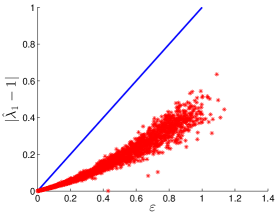
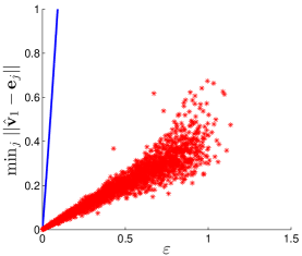
Perturbation: binary
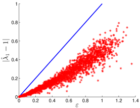
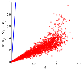
Perturbation: uniform
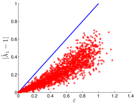
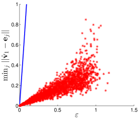
Perturbation: Gaussian

Fig. 1: Approximation Errors of the First Iteration. The approximation errors in $\hat{\lambda}_{1}$ (resp., $\hat{\bm{v}}_{1}$) are plotted on the left (resp., right) as a function of the size of the perturbation $\varepsilon$. Each (red) point corresponds to one randomly generated instance, and the (blue) solid line is the upper bound from Theorem 2.

We generate nearly symmetric orthogonally decomposable tensors $\widehat{\bm{\mathcal{T}}}=\bm{\mathcal{T}}+\bm{\mathcal{E}}\in\mathbb{R}^{10\times 10\times 10}$ in the following manner. We let the underlying symmetric orthogonally decomposable tensor $\bm{\mathcal{T}}$ be the diagonal tensor with all diagonal entries equal to one, i.e., $\bm{\mathcal{T}}=\sum_{i=1}^{10}\bm{e}_{i}^{\otimes 3}$ (where $\bm{e}_{i}$ is the $i$-th coordinate basis vector). The perturbation tensor $\bm{\mathcal{E}}$ is generated under the following three random models:

Binary:

independent entries $\mathcal{E}_{i,j,k}\in\{\pm\sigma\}$ uniformly at random;

Uniform:

indepedent entries $\mathcal{E}_{i,j,k}\in[-2\sigma,2\sigma]$ uniformly at random;

Gaussian:

independent entries $\mathcal{E}_{i,j,k}\sim\mathcal{N}(0,\sigma^{2})$;

where $\sigma$ is varied from $0.0001$ to $0.2$ with increment $0.0001$, and one instance is generated for each value of $\sigma$.

For every randomly generated instance, we solve the polynomial optimization problems

(2.12) $$\left\|\bm{\mathcal{E}}\right\| =\max_{\left\|\bm{x}\right\|=1}\bm{\mathcal{E}}\bm{x}^{\otimes 3}\quad\mbox{and}\quad\hat{\bm{v}}_{1}\in\arg\max_{\left\|\bm{x}\right\|=1}\widehat{\bm{\mathcal{T}}}\bm{x}^{\otimes 3}$$

using the general polynomial solver GloptiPoly 3 (henrion2009gloptipoly, ), and set $\hat{\lambda}_{1}:=\widehat{\bm{\mathcal{T}}}\hat{\bm{v}}_{1}^{\otimes 3}.$

In Figure 1, we plot the approximation error $|\hat{\lambda}_{1}-1|$ and $\min_{j\in[10]}\left\|\hat{\bm{v}}_{1}-\bm{e}_{j}\right\|$, respectively against the value of norm $\left\|\bm{\mathcal{E}}\right\|$. Each (red) point corresponds to one randomly generated instance, and the (blue) lines are the upper bounds given in Theorem 2. We observe no instance violating the theoretical bounds.

3 Full Decomposition Analysis

In the second iteration of Algorithm 1, we have

$$\hat{\bm{v}}_{2}\in\arg\max_{\left\|\bm{x}\right\|_{2}=1}\widehat{\bm{\mathcal{T}}}_{1}\bm{x}^{\otimes p},\quad\hat{\lambda}_{2}=\widehat{\bm{\mathcal{T}}}_{1}\hat{\bm{v}}_{2}^{\otimes p},$$

where, for some $j\in[n]$,

$$\widehat{\bm{\mathcal{T}}}_{1}=\hat{\bm{\mathcal{T}}}-\hat{\lambda}_{1}\hat{\bm{v}_{1}}^{\otimes p}=\sum_{i\neq j}\lambda_{i}\bm{v}_{i}^{\otimes p}+\widehat{\bm{\mathcal{E}}}\quad\text{and}\quad\widehat{\bm{\mathcal{E}}}=\bm{\mathcal{E}}+(\lambda_{j}\bm{v}_{j}^{\otimes p}-\hat{\lambda}_{1}\hat{\bm{v}_{1}}^{\otimes p}).$$

Theorem 2 can be directly applied again by bounding the error norm $\|\widehat{\bm{\mathcal{E}}}\|$. However, since

$$\|\widehat{\bm{\mathcal{E}}}\| =\left\|\bm{\mathcal{E}}+(\lambda_{j}\bm{v}_{j}^{\otimes p}-\hat{\lambda}_{1}\hat{\bm{v}_{1}}^{\otimes p})\right\|$$

$$=\left\|\bm{\mathcal{E}}+(\lambda_{j}-\hat{\lambda}_{1})\bm{v}_{j}^{\otimes p}+\hat{\lambda}_{1}(\bm{v}_{j}^{\otimes p}-\hat{\bm{v}}_{1}^{\otimes p})\right\|$$

$$\leq\left\|\bm{\mathcal{E}}\right\|+|\lambda_{j}-\hat{\lambda}_{1}|+\hat{\lambda}_{1}\left\|\bm{v}_{j}^{\otimes p}-\hat{\bm{v}}_{1}^{\otimes p}\right\|$$

$$\leq(2+10\sqrt{p})\varepsilon+O(\varepsilon^{2}/\lambda_{j}),$$

it appears that the approximation error may increase dramatically with the iteration number.

Fortunately, a more careful analysis shows that approximation error does not in fact accmulate in this way. The high-level reason is that while the operator norm $\|\lambda_{j}\bm{v}_{j}^{\otimes p}-\hat{\lambda}_{1}\hat{\bm{v}}_{1}^{\otimes p}\|$ is of order $\varepsilon$, the relevant quantity is essentially $\left(\lambda_{j}\bm{v}_{j}^{\otimes p}-\hat{\lambda}_{1}\hat{\bm{v}}_{1}^{\otimes p}\right)$ operating on the direction of $\hat{\bm{v}}_{2}$, i.e. $|(\lambda_{j}\bm{v}_{j}^{\otimes p}-\hat{\lambda}_{1}\hat{\bm{v}}_{1}^{\otimes p})\hat{\bm{v}}_{2}^{\otimes p}|$, which only gives rise to a quantity of order $\varepsilon^{2}$ because $p\geq 3$. This enables us to keep the approximation errors under control.

The main result of this section is as follows.

Theorem 5.

Pick any odd positive integer $p\geq 3$. There exists a positive constant $c_{0}=c_{0}(p)>0$ such that the following holds. Let $\widehat{\bm{\mathcal{T}}}:=\bm{\mathcal{T}}+\bm{\mathcal{E}}\in\bigotimes^{p}\mathbb{R}^{n}$, where $\bm{\mathcal{T}}$ is a symmetric tensor with orthogonal decomposition $\bm{\mathcal{T}}=\sum_{i=1}^{n}\lambda_{i}\bm{v}_{i}^{\otimes p}$, $\left\{\bm{v}_{1},\bm{v}_{2},\dotsc,\bm{v}_{n}\right\}$ is an orthonormal basis of $\mathbb{R}^{n}$, $\lambda_{i}>0$ for all $i\in[n]$, and $\bm{\mathcal{E}}$ is a symmetric tensor with operator norm $\varepsilon:=\left\|\bm{\mathcal{E}}\right\|$. Assume $\varepsilon\leq c_{0}\lambda_{\min}/n^{1/(p-1)}$, where $\lambda_{\min}:=\min_{i\in[n]}\lambda_{i}$. Let $\{(\hat{\lambda}_{i},\hat{\bm{v}}_{i})\}_{i\in[n]}$ be the output of Algorithm 1 for input $\widehat{\bm{\mathcal{T}}}$. Then there exists a permutation $\pi$ on $[n]$ such that

$$|\lambda_{\pi(j)}-\hat{\lambda}_{j}|\leq 2\varepsilon,\qquad\left\|\bm{v}_{\pi(j)}-\hat{\bm{v}}_{j}\right\|\leq 20\varepsilon/\lambda_{\pi(j)},\quad\forall j\in[n].$$

3.1 Deflation Analysis

The proof of Theorem 5 is based on the following lemma, which provides a careful analysis of the errors introduced in $\bm{\mathcal{T}}_{i}$ from steps $1,2,\dotsc,i$ in Algorithm 1. This lemma is a generalization of a result from JMLR:v15:anandkumar14b (which only dealt with the $p=3$ case) and also more transparently reveals the sources of errors that result from deflation.

Lemma 6.

Fix a subset $S\subseteq[n]$ and assume that $0\leq\hat{\varepsilon}\leq\lambda_{i}/2$ for each $i\in S$. Choose any $\{(\hat{\lambda}_{i},\hat{\bm{v}}_{i})\}_{i\in S}\subset\mathbb{R}\times\mathbb{R}^{n}$ such that

$$|\lambda_{i}-\hat{\lambda}_{i}|\leq\hat{\varepsilon},\quad\|\hat{\bm{v}}_{i}\|=1,\quad\text{and}\quad\left\langle\bm{v}_{i},\hat{\bm{v}}_{i}\right\rangle\geq 1-2(\hat{\varepsilon}/\lambda_{i})^{2}>0,$$

and define $\bm{\Delta}_{i}:=\lambda_{i}\bm{v}_{i}^{\otimes p}-\hat{\lambda}_{i}\hat{\bm{v}}_{i}^{\otimes p}$ for $i\in S$. Pick any unit vector $\bm{x}=\sum_{i=1}^{n}x_{i}\bm{v}_{i}$. Let $S_{1}\subseteq S$ be the indices $i\in[n]$ such that $\lambda_{i}|x_{i}|\geq 4\hat{\varepsilon}$, and let $S_{2}:=S\setminus S_{1}$. Then

(3.1) $$\left\|\sum_{i\in S_{1}}\bm{\Delta}_{i}\bm{x}^{\otimes p-1}\right\|_{2} \leq 2^{p+1}p\bigg{(}\sum_{i\in S_{1}}x_{i}^{2(p-2)}\bigg{)}^{1/2}\hat{\varepsilon}+2^{p+1}\sum_{i\in S_{1}}|x_{i}|^{p-1}\hat{\varepsilon},$$

(3.2) $$\left\|\sum_{i\in S_{2}}\bm{\Delta}_{i}\bm{x}^{\otimes p-1}\right\|_{2} \leq 6^{p}\left(\sum_{i\in S_{2}}\left(\frac{\hat{\varepsilon}}{\lambda_{i}}\right)^{2(p-2)}\right)^{1/2}\hat{\varepsilon}+6^{p}\sum_{i\in S_{2}}\left(\frac{\hat{\varepsilon}}{\lambda_{i}}\right)^{p-1}\hat{\varepsilon}.$$

These imply that there exists positive constants $c_{1},c_{2}>0$, depending only on $p$, such that

(3.3) $$\left\|\sum_{i\in S_{1}}\bm{\Delta}_{i}\bm{x}^{\otimes p-1}\right\|_{2} \leq c_{1}\cdot\left(\sum_{i\in S_{1}}|x_{i}|^{p-1}\hat{\varepsilon}\right),$$

(3.4) $$\left\|\sum_{i\in S_{2}}\bm{\Delta}_{i}\bm{x}^{\otimes p-1}\right\|_{2} \leq c_{2}\cdot\left(\sum_{i\in S_{2}}\left(\frac{\hat{\varepsilon}}{\lambda_{i}}\right)^{p-1}\hat{\varepsilon}\right),$$

(3.5) $$\left\|\sum_{i\in S_{\hphantom{1}}}\bm{\Delta}_{i}\bm{x}^{\otimes p-1}\right\|_{2} \leq c_{1}\cdot\left(\sum_{i\in S}|x_{i}|^{p-1}\hat{\varepsilon}\right)+c_{2}\cdot\left(|S|\left(\frac{\hat{\varepsilon}}{\min_{i\in S}\lambda_{i}}\right)^{p-1}\hat{\varepsilon}\right).$$

Remark 3.

Lemma 6 indicates that the accumulating error $\sum_{i\in S}\bm{\Delta}_{i}$ much less severely affects vectors that are incoherent with $\left\{\bm{v}_{i}:i\in S\right\}$. For instance, $\left\|\sum_{i\in S}\bm{\Delta}_{i}\bm{v}_{i}^{\otimes p-1}\right\|=O(\hat{\varepsilon}^{2})$ for $i\in[n]\setminus S$, while $\left\|\sum_{i\in S}\bm{\Delta}_{i}\bm{v}_{i}^{\otimes p-1}\right\|=O(\hat{\varepsilon})$ for $i\in S$.

3.2 Proof of Main Theorem

We now use Lemma 6 to prove the main theorem.

Proof of Theorem 5.

It suffices to prove that the following property holds for each $i\in[n]$:

($$* \text{there is a permutation $\pi$ on $[i]$ s.t., for all $j\in[i]$},\ \begin{cases}|\lambda_{\pi(j)}-\hat{\lambda}_{j}|\leq 2\varepsilon,\ \text{and}\\ \left\|\bm{v}_{\pi(j)}-\hat{\bm{v}}_{j}\right\|\leq\frac{20\varepsilon}{\lambda_{\pi(j)}}.\end{cases}$$)

The proof is by induction. The base case of ($*$ ‣ 3.2) (where $i=1$) follows directly from by Theorem 2.

Assume the induction hypothesis  ($*$ ‣ 3.2) is true for some $i\in[n-1]$. We will prove that there exists an $l\in[n]\setminus\{\pi(j):j\in[i]\}$ that satisfies

(3.6) $$|\lambda_{l}-\hat{\lambda}_{i+1}|\leq 2\varepsilon,\quad\left\|\bm{v}_{l}-\hat{\bm{v}}_{i+1}\right\|\leq 20\varepsilon/\lambda_{l}.$$

To simplify notation, we assume without loss of generality (by renumbering indices) that $\pi(j)=j$ for each $j\in[i]$. Let $\hat{\bm{x}}=\sum_{i\in[n]}x_{i}\bm{v}_{i}:=\hat{\bm{v}}_{i+1}$ and $\hat{\lambda}:=\hat{\lambda}_{i+1}$, and further assume without loss of generality (again by renumbering indices) that

$$\lambda_{i+1}|x_{i+1}|^{p-2}\geq\lambda_{i+2}|x_{i+2}|^{p-2}\geq\dotsb\geq\lambda_{n}|x_{n}|^{p-2}.$$

In the following, we will show that $l=i+1$ is an index satisfying (3.6). We use the assumption that

(3.7) $$\varepsilon<\min\left\{\frac{1}{8},\,\frac{1}{2.5+10c_{1}},\,\frac{1}{10(40c_{2}n)^{1/(p-1)}}\right\}\cdot\lambda_{\min}$$

(which holds with a suitable choice of $c_{0}$ in the theorem statement). Here, $c_{1}$ and $c_{2}$ are the constants from Lemma 6 when $\hat{\varepsilon}=10\varepsilon$. It can be verified that ($*$ ‣ 3.2) implies that the conditions for Lemma 6 are satisfied with this value of $\hat{\varepsilon}$.

Recall that $\hat{\lambda}=\widehat{\bm{\mathcal{T}}}_{i}\hat{\bm{x}}^{\otimes p}$, where

$$\widehat{\bm{\mathcal{T}}}_{i}=\widehat{\bm{\mathcal{T}}}-\sum_{j=1}^{i}\hat{\lambda}_{j}\hat{\bm{v}}_{j}^{\otimes p}=\sum_{j=i+1}^{n}\lambda_{j}\bm{v}_{j}^{\otimes p}+\bm{\mathcal{E}}+\sum_{j=1}^{i}\bm{\Delta}_{j}.$$

We now bound $\hat{\lambda}$ from above and below. For the lower bound, we use (3.4) from Lemma 6 to obtain

(3.8) $$\hat{\lambda} =\widehat{\bm{\mathcal{T}}}_{i}\hat{\bm{x}}^{\otimes p}\geq\max_{j\in[n]\setminus[i]}\widehat{\bm{\mathcal{T}}}_{i}{\bm{v}_{j}}^{\otimes p}\geq\lambda_{\max,i}-\varepsilon-c_{2}n\left(\frac{10\varepsilon}{\lambda_{\min}}\right)^{p-1}\varepsilon\geq\lambda_{\max,i}-1.25\varepsilon$$

where $\lambda_{\max,i}:=\max_{j\in[n]\setminus[i]}\lambda_{j}$ and $\lambda_{\min}:=\min_{j\in[n]}\lambda_{j}$; the final inequality uses the conditions on $\varepsilon$ in (3.7). For the upper bound, we have

$$\hat{\lambda}=\widehat{\bm{\mathcal{T}}}_{i}\hat{\bm{x}}^{\otimes p} =\sum_{j=i+1}^{n}\lambda_{i}x_{i}^{p}+\bm{\mathcal{E}}\hat{\bm{x}}^{\otimes p}+\sum_{j=1}^{i}\bm{\Delta}_{j}\hat{\bm{x}}^{\otimes p}$$

$$\leq\sum_{j=i+1}^{n}\lambda_{j}x_{j}^{p}+\varepsilon+10c_{1}\sum_{j=1}^{i}|x_{j}|^{p-1}\varepsilon+10c_{2}n\left(\frac{10\varepsilon}{\lambda_{\min}}\right)^{p-1}\varepsilon$$

$$\leq\lambda_{i+1}|x_{i+1}|^{p-2}\sum_{j=i+1}^{n}x_{j}^{2}+\varepsilon+10c_{1}\varepsilon\sum_{j=1}^{i}x_{j}^{2}+10c_{2}n\left(\frac{10\varepsilon}{\lambda_{\min}}\right)^{p-1}\varepsilon$$

(3.9) $$\leq\max\left\{\lambda_{i+1}|x_{i+1}|^{p-2},\,10c_{1}\varepsilon\right\}+1.25\varepsilon.$$

The first inequality above follows from (3.5) in Lemma 6; the third inequality uses the fact that $\sum_{j=1}^{n}x_{j}^{2}=1$ as well as the conditions on $\varepsilon$ in (3.7). If the $\max$ is achieved by the second argument $10c_{1}\varepsilon$, then combining (3.8) and (3.9) gives

$$(2.5+10c_{1})\varepsilon\geq\lambda_{\max,i}\geq\lambda_{\min},$$

a contradiction of (3.7). Therefore the $\max$ in (3.9) must be achieved by $\lambda_{i+1}|x_{i+1}|^{p-2}$, and hence combining (3.8) and (3.9) gives

$$\lambda_{i+1}|x_{i+1}|^{p-2}\geq\lambda_{\max,i}-2.5\varepsilon\quad\text{and}\quad|\hat{\lambda}-\lambda_{i+1}|\leq 1.25\varepsilon.$$

This in turn implies that

(3.10) $$|x_{i+1}|\geq|x_{i+1}|^{p-2}\geq 1-\frac{2.5\varepsilon}{\lambda_{i+1}},\quad\lambda_{i+1}\geq\lambda_{\max,i}-2.5\varepsilon,\quad\text{and}\quad x_{i+1}^{2}\geq x_{i+1}^{p-1}\geq 1-\frac{5\varepsilon}{\lambda_{i+1}}.$$

Thus, we have shown that $\hat{\bm{x}}$ is indeed coherent with $\hat{\bm{v}}_{i+1}$. Next, we will sharpen the bound for $\left\|\hat{\bm{x}}-\hat{\bm{v}}_{i+1}\right\|$ by considering the first order optimality condition.

Since $\hat{\bm{x}}\in\arg\min_{\left\|\bm{x}\right\|_{2}=1}\widehat{\bm{\mathcal{T}}}_{i}\bm{x}^{\otimes p}$, a first-order optimality condition similar to (2.7) implies $\hat{\lambda}=\widehat{\bm{\mathcal{T}}}_{i}\hat{\bm{x}}^{\otimes p}$. Thus

$$\hat{\lambda}\hat{\bm{x}}=\widehat{\bm{\mathcal{T}}}_{i}\hat{\bm{x}}^{\otimes p-1} =\left(\sum_{j=i+1}^{n}\lambda_{j}\bm{v}_{j}^{\otimes p}+\bm{\mathcal{E}}+\sum_{j=1}^{i}\bm{\Delta}_{j}\right)\hat{\bm{x}}^{\otimes p-1}$$

$$=\lambda_{i+1}x_{i+1}^{p-1}\bm{v}_{i+1}+\sum_{j=i+2}^{n}\lambda_{j}x_{j}^{p-1}\bm{v}_{j}+\bm{\mathcal{E}}\hat{\bm{x}}^{\otimes p-1}+\sum_{j=1}^{i}\bm{\Delta}_{j}\hat{\bm{x}}^{\otimes p-1}.$$

Therefore

$$\left\|\lambda_{i+1}(\hat{\bm{x}}-\bm{v}_{i+1})\right\|_{2}$$

$$=\left\|(\lambda_{i+1}-\hat{\lambda})\hat{\bm{x}}+(\hat{\lambda}\hat{\bm{x}}-\lambda_{i+1}\bm{v}_{i+1})\right\|_{2}$$

$$=\left\|(\lambda_{i+1}-\hat{\lambda})\hat{\bm{x}}+\lambda_{i+1}(x_{i+1}^{p-1}-1)\bm{v}_{i+1}+\sum_{j=i+2}^{n}\lambda_{j}x_{j}^{p-1}\bm{v}_{j}+\bm{\mathcal{E}}\hat{\bm{x}}^{\otimes p-1}+\sum_{j=1}^{i}\bm{\Delta}_{j}\hat{\bm{x}}^{\otimes p-1}\right\|_{2}$$

(3.11) $$\leq|\lambda_{i+1}-\hat{\lambda}|+\lambda_{i+1}|x_{i+1}^{p-1}-1|+\left\|\sum_{j=i+2}^{n}\lambda_{j}x_{j}^{p-1}\bm{v}_{j}\right\|_{2}+\left\|\bm{\mathcal{E}}\hat{\bm{x}}^{\otimes p-1}\right\|_{2}+\left\|\sum_{j=1}^{i}\bm{\Delta}_{j}\hat{\bm{x}}^{\otimes p-1}\right\|_{2}.$$

For the third term in (3.11), we use the fact that $|x_{i+2}|\leq\sqrt{1-x_{i+1}^{2}}$, the bounds from (3.10) and the conditions on $\varepsilon$ in (3.7) to obtain

$$\left\|\sum_{j=i+2}^{n}\lambda_{j}x_{j}^{p-1}\bm{v}_{j}\right\|_{2} =\left(\sum_{j=i+2}^{n}\lambda_{j}^{2}x_{j}^{2p-2}\right)^{1/2}$$

$$\leq\lambda_{i+2}|x_{i+2}|^{p-2}\sqrt{1-x_{i+1}^{2}}$$

$$\leq\lambda_{i+2}(1-x_{i+1}^{2})$$

$$\leq\lambda_{\max,i}\frac{5\varepsilon}{\lambda_{i+1}}$$

$$\leq\frac{5\varepsilon}{1-2.5\varepsilon/\lambda_{\max,i}}$$

(3.12) $$\leq 7.5\varepsilon.$$

For the last term in (3.11), we use (3.5) from Lemma 6 and the conditions on $\varepsilon$ in (3.7) to get

$$\left\|\sum_{j=1}^{i}\bm{\Delta}_{j}\hat{\bm{x}}^{\otimes p-1}\right\|_{2} \leq 10c_{1}\sum_{j=1}^{n}|x_{j}|^{p-1}\varepsilon+10c_{2}n\left(\frac{10\varepsilon}{\lambda_{\min}}\right)^{p-1}\varepsilon$$

$$\leq 10c_{1}(1-x_{i+1}^{2})\varepsilon+10c_{2}n\left(\frac{10\varepsilon}{\lambda_{\min}}\right)^{p-1}\varepsilon$$

$$\leq\frac{50c_{1}}{\lambda_{i+1}}\varepsilon^{2}+0.25\varepsilon$$

(3.13) $$\leq 5.25\varepsilon.$$

Therefore, substituting (3.10), (3.13) and $\left\|\bm{\mathcal{E}}\right\|\leq\varepsilon$ into (3.11) gives

$$\left\|\lambda_{i+1}(\hat{\bm{x}}-\bm{v}_{i+1})\right\|_{2}\leq 20\varepsilon.$$

∎

3.3 Stability of Full Decomposition

Theorem 5 states a (perhaps unexpected) phenomenon that the approximation errors do not accumulate with iteration number, whenever the perturbation error is small enough. In this subsection, we numerically corroborate this fact.

We generate nearly symmetric orthogonally decomposable tensors $\widehat{\bm{\mathcal{T}}}=\bm{\mathcal{T}}+\bm{\mathcal{E}}\in\mathbb{R}^{10\times 10\times 10}$ as follows. We construct the underlying symmetric orthogonally decomposable tensor $\bm{\mathcal{T}}$ as the diagonal tensor with all diagonal entries equal to one, i.e., $\bm{\mathcal{T}}=\sum_{i=1}^{10}\bm{e}_{i}^{\otimes 3}$ (where $\bm{e}_{i}$ is the $i$-th coordinate basis vector). The perturbation tensor $\bm{\mathcal{E}}$ is generated under three random models with $\sigma=0.01$:

Binary:

independent entries $\mathcal{E}_{i,j,k}\in\{\pm\sigma\}$ uniformly at random;

Uniform:

indepedent entries $\mathcal{E}_{i,j,k}\in[-2\sigma,2\sigma]$ uniformly at random;

Gaussian:

independent entries $\mathcal{E}_{i,j,k}\sim\mathcal{N}(0,\sigma^{2})$.

For each random model, we generate $500$ random instances, and apply Algorithm 1 to each $\widehat{\bm{\mathcal{T}}}$ to obtain approximate pairs $\{(\hat{\lambda}_{i},\hat{\bm{v}}_{i})\}_{i\in[10]}$. Again, we use GloptiPoly 3 to solve the polynomial optimization problem in Algorithm 1.

In Figure 2, we plot the mean and the standard deviation of the approximation errors for $\hat{\lambda}_{i}$ and $\hat{\bm{v}}_{i}$ from the $500$ random instances (for each $i\in[10]$). These indeed do not appear to grow or accumulate as the iteration number increases. This is consistent with our results in Theorem 5.

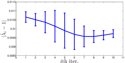
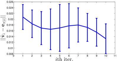
Perturbation: binary
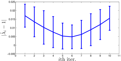
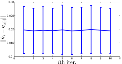
Perturbation: uniform
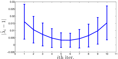
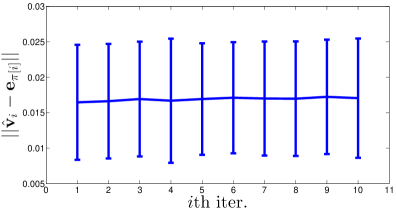
Perturbation: Gaussian

Fig. 2: Approximation Errors of Algorithm 1. For each vertical bar over the iteration index $i\in[10]$, the midpoint is the mean of the approximation errors of $\hat{\lambda}_{i}$ (left) and $\hat{\bm{v}}_{i}$ (right), computed over 500 randomly generated instances. The error bars extend to two standard deviations above and below the mean.

3.4 When $p$ is Even

We now briefly discuss the case where the order of the tensor is even, i.e., $p\geq 4$ is an even integer.

Let $\widehat{\bm{\mathcal{T}}}:=\bm{\mathcal{T}}+\bm{\mathcal{E}}\in\bigotimes^{p}\mathbb{R}^{n}$, where $\bm{\mathcal{T}}$ is a symmetric tensor with orthogonal decomposition $\bm{\mathcal{T}}=\sum_{i=1}^{n}\lambda_{i}\bm{v}_{i}^{\otimes p}$, where $\left\{\bm{v}_{1},\bm{v}_{2},\dotsc,\bm{v}_{n}\right\}$ is an orthonormal basis of $\mathbb{R}^{n}$, $\lambda_{i}\neq 0$ for all $i\in[n]$, and $\bm{\mathcal{E}}$ is a symmetric tensor with operator norm $\varepsilon:=\left\|\bm{\mathcal{E}}\right\|$. Note that unlike the case when $p$ is odd, we cannot assume $\lambda_{i}>0$ for all $i\in[n]$, and correspondingly, line 3 in Algorithm 1 now becomes

$$\hat{\bm{v}}_{i}\in\operatorname*{arg\,max}_{\left\|\bm{v}\right\|=1}\left|\widehat{\bm{\mathcal{T}}}_{i-1}\bm{v}^{\otimes p}\right|=\operatorname*{arg\,max}_{\left\|\bm{v}\right\|=1}\;\max\left\{\widehat{\bm{\mathcal{T}}}_{i-1}\bm{v}^{\otimes p},-\widehat{\bm{\mathcal{T}}}_{i-1}\bm{v}^{\otimes p}\right\},\quad\hat{\lambda}_{i}=\widehat{\bm{\mathcal{T}}}_{i-1}\hat{\bm{v}}_{i}^{\otimes p}.$$

Nevertheless, the pair $(\hat{\lambda}_{i},\hat{\bm{v}}_{i})$ still satisfies the first-order optimality condition $\hat{\lambda}_{i}\hat{\bm{v}}_{i}=\widehat{\bm{\mathcal{T}}}\hat{\bm{v}}_{i}^{\otimes p-1}$.

Our proof for Theorem 5 can be easily modified and leads to the following result: there exists a positive constant $\hat{c}_{0}=\hat{c}_{0}(p)>0$ such that whenever $\varepsilon\leq\hat{c}_{0}\left(\min_{i\in[n]}|\lambda_{i}|\right)/n^{1/(p-1)}$, there exists a permutation $\pi$ on $[n]$ such that

$$|\lambda_{\pi(j)}-\hat{\lambda}_{j}|\leq 2\varepsilon,\qquad\min\left\{\left\|\bm{v}_{\pi(j)}-\hat{\bm{v}}_{j}\right\|,\left\|\bm{v}_{\pi(j)}+\hat{\bm{v}}_{j}\right\|\right\}\leq 20\varepsilon/|\lambda_{\pi(j)}|,\quad\forall j\in[n].$$

4 Conclusion

This paper sheds light on a problem at the intersection of numerical linear algebra and statistical estimation, and our results draw upon and enrich the literature in both areas.

From the perspective of numerical linear algebra, SROA was previously only known to exactly recover the symmetric canonical decomposition of an orthogonal decomposable tensor. Our results show that it can robustly recover (approximate) orthogonal decompositions even when applied to nearly SOD tensors; this substantially enlarges the applicability of SROA.

Previous work on statistical estimation via orthogonal tensor decompositions considered the specific randomized power iteration algorithm of JMLR:v15:anandkumar14b , which has been successfully applied in a number of contexts chaganty2013linear ; ZHPA13-contrast ; azar2013bandit ; huang2013hmm ; AGHK14-community ; doshi2014graph . Our results provide formal justification for using other rank-one approximation methods in these contexts, and it seems to be quite beneficial, in terms of sample complexity and statistical efficiency, to use more sophisticated methods. Specifically, the perturbation error $\left\|\bm{\mathcal{E}}\right\|$ that can be tolerated is relaxed from power iteration’s $O(1/n)$ to $O(1/\sqrt[p-1]{n})$. In future work, we plan to empirically investigate these potential benefits in a number of applications.

We also note that solvers for rank-one tensor approximation often lack rigorous runtime or error analyses, which is not surprising given the computational difficulty of the problem for general tensors (hillar2009most, ). However, tensors that arise in applications are often more structured, such as being nearly SOD. Thus, another promising future research direction is to sidestep computational hardness barriers by developing and analyzing methods for such specially structured tensors (see also JMLR:v15:anandkumar14b ; barak2014dictionary for ideas along this line).

Appendix A Proof of Theorem 1

Since $\widehat{\bm{M}}$ is symmetric, it has an eigenvalue decomposition $\sum_{i=1}^{n}\hat{\lambda}_{i}\hat{\bm{v}}_{i}\hat{\bm{v}}_{i}^{\scriptscriptstyle{\top}}$, where $|\hat{\lambda}_{1}|\geq|\hat{\lambda}_{2}|\geq\dotsb\geq|\hat{\lambda}_{n}|$ and $\{\hat{\bm{v}}_{1},\hat{\bm{v}}_{2},\dotsc,\hat{\bm{v}}_{n}\}$ are orthonormal. It is straightforward to obtain:

$$\hat{\lambda}=\hat{\lambda}_{1}\quad\text{and}\quad\widehat{\bm{M}}\hat{\bm{x}}=\hat{\lambda}\hat{\bm{x}}.$$

By Weyl’s inequality weyl1912asymptotische ,

$$|\hat{\lambda}-\lambda_{1}|\leq\left\|\bm{E}\right\|=\varepsilon.$$

To bound $\left\langle\hat{\bm{x}},\bm{v}_{1}\right\rangle^{2}$, we employ an argument very similar to one from davis1970rotation . Observe that

$$\left\|\bm{M}\hat{\bm{x}}-\lambda_{1}\hat{\bm{x}}\right\|^{2}=\left\|(\hat{\lambda}-\lambda_{1})\hat{\bm{x}}-\bm{E}\hat{\bm{x}}\right\|^{2}\leq(|\hat{\lambda}-\lambda_{1}|\left\|\hat{\bm{x}}\right\|+\left\|\bm{E}\hat{\bm{x}}\right\|)^{2}\leq 4\varepsilon^{2}.$$

Moreover,

$$\bm{M}\hat{\bm{x}}-\lambda_{1}\hat{\bm{x}}=\sum_{i=1}^{n}(\lambda_{i}-\lambda_{1})\left\langle\bm{v}_{i},\hat{\bm{x}}\right\rangle\bm{v}_{i}=\sum_{i=2}^{n}(\lambda_{i}-\lambda_{1})\left\langle\bm{v}_{i},\hat{\bm{x}}\right\rangle\bm{v}_{i},$$

and therefore

$$\left\|\bm{M}\hat{\bm{x}}-\lambda_{1}\hat{\bm{x}}\right\|^{2}=\sum_{i=2}^{n}(\lambda_{i}-\lambda_{1})^{2}\left\langle\bm{v}_{i},\hat{\bm{x}}\right\rangle^{2}\geq\gamma^{2}\sum_{i=2}^{n}\left\langle\bm{v}_{i},\hat{\bm{x}}\right\rangle^{2}=\gamma^{2}(1-\left\langle\bm{v}_{i},\hat{\bm{x}}\right\rangle^{2}).$$

Combining the upper and lower bounds on $\left\|\bm{M}\hat{\bm{x}}-\lambda_{1}\hat{\bm{x}}\right\|^{2}$ gives $\left\langle\hat{\bm{x}},\bm{v}_{1}\right\rangle^{2}\geq 1-(2\varepsilon/\gamma)^{2}$ as claimed. ∎

Appendix B Proof of Lemma 6

Proof.

The lemma holds trivially if $\hat{\varepsilon}=0$. So we may assume $\hat{\varepsilon}>0$. Therefore, for every $i\in S_{1}$, we have $|x_{i}|\geq 4\hat{\varepsilon}/\lambda_{i}>0$. Let $c_{i}:=\left\langle\bm{v}_{i},\hat{\bm{v}}_{i}\right\rangle$, $\bm{w}_{i}:=(\hat{\bm{v}}_{i}-c_{i}\bm{v}_{i})/\left\|\hat{\bm{v}}_{i}-c_{i}\bm{v}_{i}\right\|_{2}$, and $y_{i}:=\left\langle\bm{w}_{i},\bm{x}\right\rangle$, so

$$\hat{\bm{v}}_{i}=c_{i}\bm{v}_{i}+\sqrt{1-c_{i}^{2}}\bm{w}_{i}\quad\text{and}\quad\left\langle\hat{\bm{v}}_{i},\bm{x}\right\rangle=c_{i}x_{i}+\sqrt{1-c_{i}^{2}}y_{i}.$$

We first establish a few inequalities that will be frequently used later. Since $|\lambda_{i}-\hat{\lambda}_{i}|\leq\hat{\varepsilon}\leq\lambda_{i}/2$, one has $\hat{\varepsilon}/\lambda_{i}\leq 1/2$, and $1/2\leq\hat{\lambda}_{i}/\lambda_{i}\leq 3/2$. Also, since $c_{i}\geq 1-2(\hat{\varepsilon}/\lambda_{i})^{2}\geq 1/2$,

$$\sqrt{1-c_{i}^{2}} \leq\sqrt{1-\left(1-2\left(\hat{\varepsilon}/\lambda_{i}\right)^{2}\right)^{2}}=\sqrt{4\left(\hat{\varepsilon}/\lambda_{i}\right)^{2}\left(1-\left(\hat{\varepsilon}/\lambda_{i}\right)^{2}\right)}\leq 2\hat{\varepsilon}/\lambda_{i}.$$

For each $i\in S$,

$$\bm{\Delta}_{i}\bm{x}^{\otimes p-1}$$

$$=\left(\lambda_{i}\bm{v}_{i}^{\otimes p}-\hat{\lambda}_{i}\hat{\bm{v}}_{i}^{\otimes p}\right)\bm{x}^{\otimes p-1}$$

$$=\lambda_{i}x_{i}^{p-1}\bm{v}_{i}-\hat{\lambda}_{i}\left\langle\hat{\bm{v}}_{i},\bm{x}\right\rangle^{p-1}\hat{\bm{v}}_{i}$$

$$=\lambda_{i}x_{i}^{p-1}\bm{v}_{i}-\hat{\lambda}_{i}\left(c_{i}x_{i}+\sqrt{1-c_{i}^{2}}y_{i}\right)^{p-1}\left(c_{i}\bm{v}_{i}+\sqrt{1-c_{i}^{2}}\bm{w}_{i}\right)$$

$$=\left(\lambda_{i}x_{i}^{p-1}-\hat{\lambda}_{i}c_{i}\left(c_{i}x_{i}+\sqrt{1-c_{i}^{2}}y_{i}\right)^{p-1}\right)\bm{v}_{i}-\left(\hat{\lambda}_{i}\sqrt{1-c_{i}^{2}}\left(c_{i}x_{i}+\sqrt{1-c_{i}^{2}}y_{i}\right)^{p-1}\right)\bm{w}_{i}.$$

Therefore, due to the orthonormality of $\{\bm{v}_{i}\}_{i\in[n]}$ and the triangle inequality, for each $j\in\{1,2\}$,

(B.1) $$\left\|\sum_{i\in S_{j}}\bm{\Delta}_{i}\bm{x}^{\otimes p-1}\right\|_{2} \leq\left(\sum_{i\in S_{j}}\left(\lambda_{i}x_{i}^{p-1}-\hat{\lambda}_{i}c_{i}\left(c_{i}x_{i}+\sqrt{1-c_{i}^{2}}y_{i}\right)^{p-1}\right)^{2}\right)^{1/2}$$

$$\quad+\sum_{i\in S_{j}}\left|\hat{\lambda}_{i}\sqrt{1-c_{i}^{2}}\left(c_{i}x_{i}+\sqrt{1-c_{i}^{2}}y_{i}\right)^{p-1}\right|.$$

We now prove (3.1). For any $i\in S_{1}$, since $x_{i}\neq 0$, we may write (B.1) as

(B.2) $$\begin{aligned} \left\|\sum_{i\in S_{1}}\bm{\Delta}_{i}\bm{x}^{\otimes p-1}\right\|_{2}&\leq\left(\sum_{i\in S_{1}}x_{i}^{2p-4}\left(\lambda_{i}x_{i}-\hat{\lambda}_{i}x_{i}c_{i}^{p}\left(1+\sqrt{\frac{1-c_{i}^{2}}{c_{i}^{2}}}\frac{y_{i}}{x_{i}}\right)^{p-1}\right)^{2}\right)^{1/2}\\ &\quad+\sum_{i\in S_{1}}\left|\hat{\lambda}_{i}x_{i}^{p-1}c_{i}^{p-1}\sqrt{1-c_{i}^{2}}\left(1+\sqrt{\frac{1-c_{i}^{2}}{c_{i}^{2}}}\frac{y_{i}}{x_{i}}\right)^{p-1}\right|.\end{aligned}$$

Observe that

$$\left|\sqrt{\frac{1-c_{i}^{2}}{c_{i}^{2}}}\frac{y_{i}}{x_{i}}\right|\leq\frac{\sqrt{1-c_{i}^{2}}}{|c_{i}|}\frac{1}{|x_{i}|}\leq\frac{4\hat{\varepsilon}}{\lambda_{i}|x_{i}|}\leq 1$$

because $|c_{i}|\geq 1/2$ and $\sqrt{1-c_{i}^{2}}\geq 2\hat{\varepsilon}/\lambda_{i}$. Moreover, since $1+(p-1)z\leq(1+z)^{p-1}\leq 1+(2^{p-1}-1)z$ for any $z\in[0,1]$,

(B.3) $$\left|\left(1+\sqrt{\frac{1-c_{i}^{2}}{c_{i}^{2}}}\frac{y_{i}}{x_{i}}\right)^{p-1}-1\right|\leq(2^{p-1}-1)\frac{4\hat{\varepsilon}}{\lambda_{i}|x_{i}|}=(2^{p+1}-4)\frac{\hat{\varepsilon}}{\lambda_{i}|x_{i}|}.$$

Therefore,

$$\left|\lambda_{i}x_{i}-\hat{\lambda}_{i}x_{i}c_{i}^{p}\left(1+\sqrt{\frac{1-c_{i}^{2}}{c_{i}^{2}}}\frac{y_{i}}{x_{i}}\right)^{p-1}\right| \leq|\lambda_{i}x_{i}-\hat{\lambda}_{i}x_{i}|+\hat{\lambda}_{i}|x_{i}|\left|1-c_{i}^{p}\left(1+\sqrt{\frac{1-c_{i}^{2}}{c_{i}^{2}}}\frac{y_{i}}{x_{i}}\right)^{p-1}\right|$$

$$\leq\hat{\varepsilon}+\frac{\hat{\lambda}_{i}|x_{i}|}{\lambda_{i}}\left((2^{p+1}-4)\frac{\hat{\varepsilon}}{|x_{i}|}+p\hat{\varepsilon}+(2^{p+1}-4)\frac{\hat{\varepsilon}}{|x_{i}|}\frac{p\hat{\varepsilon}}{\lambda_{i}}\right)$$

$$\leq\hat{\varepsilon}+\frac{3}{2}\left((2^{p+1}-4)+p+(2^{p-1}-1)p\right)\hat{\varepsilon}$$

(B.4) $$\leq 2^{p+1}p\hat{\varepsilon}.$$

The second inequality above is obtained using the inequality $|(1+a)(1+b)-1|\leq|a|+|b|+|ab|$ for any $a,b\in\mathbb{R}$, together with the inequality from (B.3) and the fact $|1-c_{i}^{p}|\leq 2p(\hat{\varepsilon}/\lambda_{i})^{2}\leq p(\hat{\varepsilon}/\lambda_{i})$. Using the resulting inequality in (B.4), the first summand in (B.2) can be bounded as

(B.5) $$\left(\sum_{i\in S_{1}}x_{i}^{2p-2}\left(\lambda_{i}-\hat{\lambda}_{i}c_{i}^{p}\left(1+\sqrt{\frac{1-c_{i}^{2}}{c_{i}^{2}}}\frac{y_{i}}{x_{i}}\right)^{p-1}\right)^{2}\right)^{1/2}\leq 2^{p+1}p\left(\sum_{i\in S_{1}}x_{i}^{2(p-2)}\right)^{1/2}\hat{\varepsilon}.$$

To bound the second summand in (B.2), we have

$$\sum_{i\in S_{1}}\left|\hat{\lambda}_{i}x_{i}^{p-1}c_{i}^{p-1}\sqrt{1-c_{i}^{2}}\left(1+\sqrt{\frac{1-c_{i}^{2}}{c_{i}^{2}}}\frac{y_{i}}{x_{i}}\right)^{p-1}\right| \leq\sum_{i\in S_{1}}\left|\hat{\lambda}_{i}x_{i}^{p-1}\sqrt{1-c_{i}^{2}}\left(1+\frac{\sqrt{1-c_{i}^{2}}}{c_{i}}\frac{1}{|x_{i}|}\right)^{p-1}\right|$$

$$\leq\sum_{i\in S_{1}}\left|\hat{\lambda}_{i}x_{i}^{p-1}\frac{2\hat{\varepsilon}}{\lambda_{i}}\left(1+\frac{4\hat{\varepsilon}}{\lambda_{i}|x_{i}|}\right)^{p-1}\right|$$

(B.6) $$\leq 2^{p+1}\sum_{i\in S_{1}}|x_{i}|^{p-1}\hat{\varepsilon},.$$

The second inequality uses the facts $c_{i}\geq 1/2$ and $\sqrt{1-c_{i}^{2}}\leq 2\hat{\varepsilon}/\lambda_{i}$; the last inequality uses the facts $\hat{\lambda}_{i}/\lambda_{i}\leq 3/2$ and $\lambda_{i}|x_{i}|\geq 4\hat{\varepsilon}$. Combining (B.5) and (B.6) gives the claimed inequality in (3.1) via (B.2).

It remains to prove (3.2). For each $i\in S_{2}$,

$$\left|\lambda_{i}x_{i}^{p-1}-\hat{\lambda}_{i}c_{i}\left(c_{i}x_{i}+\sqrt{1-c_{i}^{2}}y_{i}\right)^{p-1}\right| \leq\lambda_{i}|x_{i}|^{p-1}+\hat{\lambda}_{i}\left(|x_{i}|+\sqrt{1-c_{i}^{2}}\right)^{p-1}$$

$$\leq\lambda_{i}\left(\frac{4\hat{\varepsilon}}{\lambda_{i}}\right)^{p-1}+\hat{\lambda}_{i}\left(\frac{4\hat{\varepsilon}}{\lambda_{i}}+\frac{2\hat{\varepsilon}}{\lambda_{i}}\right)^{p-1}$$

$$\leq\left(4^{p-1}+\frac{3}{2}\cdot 6^{p-1}\right)\left(\frac{\hat{\varepsilon}}{\lambda_{i}}\right)^{p-2}\hat{\varepsilon}$$

$$\leq 6^{p}\left(\frac{\hat{\varepsilon}}{\lambda_{i}}\right)^{p-2}\hat{\varepsilon}.$$

The second inequality uses the facts $\sqrt{1-c_{i}^{2}}\leq 2\hat{\varepsilon}/\lambda_{i}$ and $\lambda_{i}|x_{i}|<4\hat{\varepsilon}$ for all $i\in S_{2}$; the third inequality uses the fact $\hat{\lambda}_{i}/\lambda_{i}\leq 3/2$. Therefore

(B.7) $$\left(\sum_{i\in S_{2}}\left(\lambda_{i}x_{i}^{p-1}-\hat{\lambda}_{i}c_{i}\left(c_{i}x_{i}+\sqrt{1-c_{i}^{2}}y_{i}\right)^{p-1}\right)^{2}\right)^{1/2}\leq 6^{p}\left(\sum_{i\in S_{2}}\left(\frac{\hat{\varepsilon}}{\lambda_{i}}\right)^{2(p-2)}\right)^{1/2}\hat{\varepsilon}.$$

Moreover,

$$\sum_{i\in S_{2}}\left|\hat{\lambda}_{i}\sqrt{1-c_{i}^{2}}\left(c_{i}x_{i}+\sqrt{1-c_{i}^{2}}y_{i}\right)^{p-1}\right| \leq\sum_{i\in S_{2}}\left|\hat{\lambda}_{i}\sqrt{1-c_{i}^{2}}\left(|x_{i}|+\sqrt{1-c_{i}^{2}}\right)^{p-1}\right|$$

$$\leq\sum_{i\in S_{2}}\hat{\lambda}_{i}\frac{2\hat{\varepsilon}}{\lambda_{i}}\left(\frac{4\hat{\varepsilon}}{\lambda_{i}}+\frac{2\hat{\varepsilon}}{\lambda_{i}}\right)^{p-1}$$

$$\leq 3\cdot 6^{p-1}\sum_{i\in S_{2}}\left(\frac{\hat{\varepsilon}}{\lambda_{i}}\right)^{p-1}\hat{\varepsilon}$$

(B.8) $$\leq 6^{p}\sum_{i\in S_{2}}\left(\frac{\hat{\varepsilon}}{\lambda_{i}}\right)^{p-1}\hat{\varepsilon}.$$

Combining (B.7) and (B.8) establishes (3.2) via (B.1) (with $j=2$). ∎

References

- (1) C. Eckart and G. Young, “The approximation of one matrix by another of lower rank,” Psychometrika, vol. 1, pp. 211–218, 1936.
- (2) R. Harshman, “Foundations of the PARAFAC procedure: model and conditions for an ‘explanatory’ multi-mode factor analysis,” tech. rep., UCLA Working Papers in Phonetics, 1970.
- (3) P. McCullagh, Tensor Methods in Statistics. Chapman and Hall, 1987.
- (4) P. Comon, “Independent component analysis, a new concept?,” Signal processing, vol. 36, no. 3, pp. 287–314, 1994.
- (5) A. Smilde, R. Bro, and P. Geladi, Multi-way Analysis: Applications in the Chemical Sciences. Wiley, 2004.
- (6) T. G. Kolda and B. Bader, “Tensor decompositions and applications,” SIAM review, vol. 51, no. 3, pp. 455–500, 2009.
- (7) P. Comon and C. Jutten, Handbook of Blind Source Separation: Independent component analysis and applications. Academic press, 2010.
- (8) A. Anandkumar, R. Ge, D. Hsu, S. M. Kakade, and M. Telgarsky, “Tensor decompositions for learning latent variable models,” Journal of Machine Learning Research, vol. 15, pp. 2773–2832, 2014.
- (9) T. Zhang and G. Golub, “Rank-one approximation to high order tensors,” SIAM Journal on Matrix Analysis and Applications, vol. 23, no. 2, pp. 534–550, 2001.
- (10) E. Kofidis and P. A. Regalia, “On the best rank-1 approximation of higher-order supersymmetric tensors,” SIAM Journal on Matrix Analysis and Applications, vol. 23, no. 3, pp. 863–884, 2002.
- (11) T. Kolda, B. Bader, and J. Kenny, “Higher-order web link analysis using multilinear algebra,” in Fifth International Conference on Data Mining, 2005.
- (12) Y. Wang and L. Qi, “On the successive supersymmetric rank-1 decomposition of higher-order supersymmetric tensors,” Numerical Linear Algebra with Applications, vol. 14, no. 6, pp. 503–519, 2007.
- (13) C. J. Hillar and L.-H. Lim, “Most tensor problems are NP-hard,” Journal of the ACM, vol. 60, pp. 45:1–45:39, Nov. 2013.
- (14) N. Shor, “An approach to obtaining global extremums in polynomial mathematical programming problems,” Cybernetics and Systems Analysis, vol. 23, no. 5, pp. 695–700, 1987.
- (15) Y. Nesterov, “Squared functional systems and optimization problems,” High performance optimization, vol. 13, pp. 405–440, 2000.
- (16) P. A. Parrilo, Structured semidefinite programs and semialgebraic geometry methods in robustness and optimization. PhD thesis, California Institute of Technology, 2000.
- (17) J. B. Lasserre, “Global optimization with polynomials and the problem of moments,” SIAM Journal on Optimization, vol. 11, no. 3, pp. 796–817, 2001.
- (18) P. A. Parrilo, “Semidefinite programming relaxations for semialgebraic problems,” Mathematical programming, vol. 96, no. 2, pp. 293–320, 2003.
- (19) D. Henrion, J. B. Lasserre, and J. Löfberg, “Gloptipoly 3: moments, optimization and semidefinite programming,” Optimization Methods & Software, vol. 24, no. 4-5, pp. 761–779, 2009.
- (20) A. Papachristodoulou, J. Anderson, G. Valmorbida, S. Prajna, P. Seiler, and P. A. Parrilo, SOSTOOLS: Sum of squares optimization toolbox for MATLAB. http://arxiv.org/abs/1310.4716, 2013.
- (21) D. P. Bertsekas, Nonlinear programming. Athena Scientific, 1999.
- (22) S. J. Wright and J. Nocedal, Numerical optimization, vol. 2. Springer New York, 1999.
- (23) L. De Lathauwer, B. De Moor, and J. Vandewalle, “On the best rank- and rank- approximation of higher-order tensors,” SIAM Journal on Matrix Analysis and Applications, vol. 21, no. 4, pp. 1324–1342, 2000.
- (24) T. G. Kolda and J. R. Mayo, “Shifted power method for computing tensor eigenpairs,” SIAM Journal on Matrix Analysis and Applications, vol. 32, no. 4, pp. 1095–1124, 2011.
- (25) L. Han, “An unconstrained optimization approach for finding real eigenvalues of even order symmetric tensors,” arXiv preprint arXiv:1203.5150, 2012.
- (26) B. Chen, S. He, Z. Li, and S. Zhang, “Maximum block improvement and polynomial optimization,” SIAM Journal on Optimization, vol. 22, no. 1, pp. 87–107, 2012.
- (27) X. Zhang, C. Ling, and L. Qi, “The best rank-1 approximation of a symmetric tensor and related spherical optimization problems,” SIAM Journal on Matrix Analysis and Applications, vol. 33, no. 3, pp. 806–821, 2012.
- (28) C. Hao, C. Cui, and Y. Dai, “A sequential subspace projection method for extreme Z-eigenvalues of supersymmetric tensors,” Numerical Linear Algebra with Applications, 2014.
- (29) B. Jiang, S. Ma, and S. Zhang, “Tensor principal component analysis via convex optimization,” Mathematical Programming, pp. 1–35, 2014.
- (30) J. Nie and L. Wang, “Semidefinite relaxations for best rank-1 tensor approximations,” SIAM Journal on Matrix Analysis and Applications, vol. 35, no. 3, pp. 1155––1179, 2014.
- (31) Y. Yang, Q. Yang, and L. Qi, “Properties and methods for finding the best rank-one approximation to higher-order tensors,” Computational Optimization and Applications, vol. 58, no. 1, pp. 105–132, 2014.
- (32) C. Ling, J. Nie, L. Qi, and Y. Ye, “Biquadratic optimization over unit spheres and semidefinite programming relaxations,” SIAM Journal on Optimization, vol. 20, no. 3, pp. 1286–1310, 2009.
- (33) A. Stegeman and P. Comon, “Subtracting a best rank-1 approximation may increase tensor rank,” Linear Algebra and its Applications, vol. 433, no. 7, pp. 1276–1300, 2010.
- (34) T. G. Kolda, “Orthogonal tensor decompositions,” SIAM Journal on Matrix Analysis and Applications, vol. 23, no. 1, pp. 243–255, 2001.
- (35) T. G. Kolda, “A counterexample to the possibility of an extension of the Eckart-Young low-rank approximation theorem for the orthogonal rank tensor decomposition,” SIAM Journal on Matrix Analysis and Applications, vol. 24, no. 3, pp. 762–767, 2003.
- (36) A. Stegeman, “Degeneracy in candecomp/parafac and indscal explained for several three-sliced arrays with a two-valued typical rank,” Psychometrika, vol. 72, no. 4, pp. 601–619, 2007.
- (37) A. Stegeman, “Low-rank approximation of generic ptimesqtimes2 arrays and diverging components in the candecomp/parafac model,” SIAM Journal on Matrix Analysis and Applications, vol. 30, no. 3, pp. 988–1007, 2008.
- (38) V. De Silva and L.-H. Lim, “Tensor rank and the ill-posedness of the best low-rank approximation problem,” SIAM Journal on Matrix Analysis and Applications, vol. 30, no. 3, pp. 1084–1127, 2008.
- (39) L.-H. Lim and P. Comon, “Multiarray signal processing: Tensor decomposition meets compressed sensing,” Comptes Rendus Mecanique, vol. 338, no. 6, pp. 311–320, 2010.
- (40) L.-H. Lim and P. Comon, “Blind multilinear identification,” Information Theory, IEEE Transactions on, vol. 60, no. 2, pp. 1260–1280, 2014.
- (41) J. B. Kruskal, “Three-way arrays: rank and uniqueness of trilinear decompositions, with application to arithmetic complexity and statistics,” Linear Algebra and its Applications, vol. 18, no. 2, pp. 95–138, 1977.
- (42) L.-H. Lim, “Singular values and eigenvalues of tensors: a variational approach,” Proceedings of the IEEE International Workshop on Computational Advances in Multi-Sensor Adaptive Processing, vol. 1, pp. 129–132, 2005.
- (43) H. Weyl, “Das asymptotische verteilungsgesetz der eigenwerte linearer partieller differentialgleichungen (mit einer anwendung auf die theorie der hohlraumstrahlung),” Mathematische Annalen, vol. 71, no. 4, pp. 441–479, 1912.
- (44) C. Davis and W. Kahan, “The rotation of eigenvectors by a perturbation. III,” SIAM Journal on Numerical Analysis, vol. 7, no. 1, pp. 1–46, 1970.
- (45) A. T. Chaganty and P. Liang, “Spectral experts for estimating mixtures of linear regressions,” in International Conference on Machine Learning, 2013.
- (46) J. Zou, D. Hsu, D. Parkes, and R. P. Adams, “Contrastive learning using spectral methods,” in Advances in Neural Information Processing Systems 26, 2013.
- (47) M. G. Azar, A. Lazaric, and E. Brunskill, “Sequential transfer in multi-armed bandit with finite set of models,” in Advances in Neural Information Processing Systems 26, 2013.
- (48) T.-K. Huang and J. Schneider, “Learning hidden Markov models from non-sequence data via tensor decomposition,” in Advances in Neural Information Processing Systems 26, 2013.
- (49) A. Anandkumar, R. Ge, D. Hsu, and S. M. Kakade, “A tensor approach to learning mixed membership community models,” Journal of Machine Learning Research, vol. 15, no. Jun, pp. 2239–2312, 2014.
- (50) F. Doshi-Velez, B. Wallace, and R. Adams, “Graph-Sparse LDA: A Topic Model with Structured Sparsity,” ArXiv e-prints, Oct. 2014.
- (51) B. Barak, J. A. Kelner, and D. Steurer, “Dictionary learning and tensor decomposition via the sum-of-squares method,” arXiv preprint arXiv:1407.1543, 2014.