Dynamics of entanglement and transport in 1D systems with quenched randomness
Abstract
Quenched randomness can have a dramatic effect on the dynamics of isolated 1D quantum many-body systems, even for systems that thermalize. This is because transport, entanglement, and operator spreading can be hindered by ‘Griffiths’ rare regions which locally resemble the many-body-localized phase and thus act as weak links. We propose coarse-grained models for entanglement growth and for the spreading of quantum operators in the presence of such weak links. We also examine entanglement growth across a single weak link numerically. We show that these weak links have a stronger effect on entanglement growth than previously assumed: entanglement growth is sub-ballistic whenever such weak links have a power-law probability distribution at low couplings, i.e. throughout the entire thermal Griffiths phase. We argue that the probability distribution of the entanglement entropy across a cut can be understood from a simple picture in terms of a classical surface growth model. Surprisingly, the four length scales associated with (i) production of entanglement, (ii) spreading of conserved quantities, (iii) spreading of operators, and (iv) the width of the ‘front’ of a spreading operator, are characterized by dynamical exponents that in general are all distinct. Our numerical analysis of entanglement growth between weakly coupled systems may be of independent interest.
I Introduction
A basic question about a many-body quantum system, closely related to its ability to thermalize, is how effectively quantum information spreads through it. The dynamical generation of quantum entanglement, following a quantum quench from a weakly entangled state, provides one window on information spreading Calabrese and Cardy (2005); Chiara et al. (2006); Bardarson et al. (2012); Kim and Huse (2013); Nahum et al. (2016). Unitary dynamics typically generates correlations between increasingly distant degrees of freedom as time goes on. The resulting irreversible growth in the entanglement entropy of a subsystem reveals differences between integrable, nonintegrable, disordered and many-body localized (MBL) Bardarson et al. (2012); Nandkishore and Huse (2015) systems.
Complementary insight into information spreading comes from considering light-cone-like effects limiting the propagation of signals and disturbances through the system Lieb and Robinson (1972). This leads to the question of how an initially local quantum operator spreads and becomes nonlocal under Heisenberg time evolution. Again there are important differences between clean and disordered systems.
In translationally invariant one-dimensional (1D) systems, entanglement growth and operator spreading are both typically associated with nonzero speeds Calabrese and Cardy (2005); Chiara et al. (2006); Kim and Huse (2013); Nahum et al. (2016); Roberts et al. (2015). By contrast, in the MBL phase both entanglement growth Chiara et al. (2006); Žnidarič et al. (2008); Bardarson et al. (2012); Serbyn et al. (2013a); Huse et al. (2014) and operator spreading Huang et al. (2016); Fan et al. (2016); Chen (2016); Swingle and Chowdhury (2016); He and Lu (2016); Chen et al. (2016); Slagle et al. (2016) are associated with length scales that grow only logarithmically in time.
This paper studies a third situation: 1D systems that are disordered, but are in the thermalizing phase. In 1D, quenched randomness can strongly affect transport and information spreading even in the thermal phase. This is because there can exist rare regions where disorder happens to be stronger than average, and which locally resemble the MBL phase. These ‘Griffiths’ regions act as bottlenecks or weak links, hindering the propagation both of conserved quantities and of quantum information. The effects on transport are fairly well understood: strong enough disorder leads to subdiffusive transport Vosk et al. (2015); Potter et al. (2015); Agarwal et al. (2015), as observed numerically Bar Lev et al. (2015); Agarwal et al. (2015); Luitz et al. (2016); Khait et al. (2016); Žnidarič et al. (2016). (Certain rare-region effects have also been addressed experimentally Lüschen et al. (2016).) Sub-ballistic entanglement and signal propagation has been observed numerically in the Griffiths phase Luitz et al. (2016); Luitz and Lev (2017).
Here we provide long-wavelength pictures which expose the universal physics underlying entanglement growth and operator spreading in the Griffiths phase, and yield the universal scaling exponents and scaling forms governing these processes. In contrast to both clean systems and the MBL phase, we find that the lengthscales governing entanglement growth and operator growth (as measured by the so-called out-of-time-order correlator) scale with different powers of the time. In a certain sense, entanglement growth is parametrically slower than operator spreading in the Griffiths phase.
We provide a long-distance picture for entanglement entropy growth in terms of an effective classical surface growth problem. The height of the growing ‘surface’, , is the amount of entanglement across a cut in the 1D system at position ; the growth of the surface is deterministic, but it is affected by quenched randomness in the local growth rates. This picture is motivated by an analogy to a simpler quantum dynamics based on a random quantum circuit Nahum et al. (2016). The basic assumptions are also substantiated independently, including with a semi-microscopic analysis of entangling across a Griffiths region.
The surface growth picture leads to the unexpected conclusion that entanglement growth is sub-ballistic throughout the entire thermal Griffiths phase, i.e. whenever Griffiths regions locally resembling the MBL phase are possible. (This requires the absence of exact nonabelian symmetries, as these prohibit MBL Chandran et al. (2014); Potter and Vasseur (2016); Protopopov et al. (2016).) We give expressions for the dynamical exponent governing the growth of the von Neumann entropy and for the probability distribution of this quantity at late times.
Turning to operator growth, we propose a very simple ‘hydrodynamic’ picture for the out-of-time-order correlator in the Griffiths phase, making use of the random circuit results in Ref. Nahum et al. (2017) (see also von Keyserlingk et al. (2017)). We obtain a picture involving two separate diverging length scales at long times. In fact we argue that in the Griffiths phase there are in general at least four separate dynamical exponents , characterizing four length scales that can grow with time with different exponents: these are associated with entanglement growth (), with the spreading of an operator (), with the width of the ‘front’ of the OTOC (), and with spreading of conserved quantities (). (See the table in Sec. V.) In particular, ballistic spreading of operators does not imply ballistic spreading of entanglement, contrary to previous suggestions.
Studying the thermal Griffiths phase leads naturally to questions about how two weakly-coupled systems exchange quantum information. These questions are of general interest, outside the context of disordered systems. How do two weakly coupled quantum systems become entangled over time? How do operators localized in one of the systems spread across the weak link? We provide numerical and analytical results for generation of entanglement across the weak link, showing that the entanglement entropy is governed by a very simple scaling function and that the ‘weak link’ can be characterized by a well-defined entanglement growth rate. (We investigate numerically how this growth rate depends on the strength of the weak coupling and on the index of the Renyi entropy .) We propose a simple scaling form for the out-of-time-order correlator of an operator which spreads across a weak link between two semi-infinite 1D chains.
II Entanglement growth
In this section we study entanglement growth starting from a weakly entangled state: this could be the ground state of the pre-quench Hamiltonian in a quantum quench. The specific 1D system does not matter at this stage, but an archetypal example is the Heisenberg spin chain with random couplings and fields,
| (1) |
(We could also consider a Floquet spin chain with effective discrete time dynamics.) Such chains will thermalize if the randomness is not too strong. However, thermalization may be slow as a result of ‘weak links’. These may be simply weak couplings where a single bond is very weak. More robustly, the weak links may be due to extended Griffiths regions where the disorder happens to be more severe, so that MBL physics arises locally Agarwal et al. (2015).
Moving to a coarse-grained description, let us label ‘weak links’ by an index , with a given weak link located at a position . A key assumption is that each weak link has a well-defined local entanglement rate , which is the rate at which entanglement is generated across the weak link in the absence of other weak links. We will give arguments supporting this assumption in Secs. VI, VII. The local entanglement rates are assumed to be independent random variables with a power-law distribution at small :
| (2) |
The exponent depends on the strength of disorder and tends to as the many-body localization transition is approached. The power-law form arises because the probability of a Griffiths region of length , and the entangling rate associated with such a region, both decrease exponentially with (Sec. VI). Or the power law might arise directly from the ‘bare’ probability distribution of the couplings . As usual, we will neglect the weak link’s nonzero spatial extent : for Griffiths regions this grows only logarithmically as , so is negligible compared to the lengthscales discussed below which grow as powers of .
Consider a chain with open boundary conditions that is in a pure quantum many-body state, and let be the von Neumann entanglement entropy across a cut through the bond at position at time . Formally,
| (3) |
where the subsystem contains the degrees of freedom to the left of (Fig. 2). We could also consider a mixed state of the full system, in which case this is the von Neumann entropy of the subsystem to the left of the cut.
We will model the dynamics of as deterministic surface growth. In the next subsection we will motivate this using a toy model for entanglement growth in the presence of weak links, but first we describe the consequences for the coarse-grained dynamics.
The surface growth picture takes into account two crucial physical constraints. First, the growth rate at a weak link is constrained by the local rate . Second, the spatial slope of the entropy profile is constrained by the density of active degrees of freedom in the spin chain:
| (4) |
Here is the entropy density of the thermal state to which the system is locally equilibrating. The second inequality follows from subadditivity of the von Neumman entropy, together with the assumption that local reduced density matrices (for adjacent spins) thermalize at late times. In a lattice spin model at infinite temperature, is the logarithm of the local Hilbert space dimension per unit length; this version of the inequality follows rigorously from subadditivity. In the following we will rescale so that the inequality becomes
| (5) |
If the system has any conserved densities, such as energy, that have a spatial distribution that is away from thermal equilibrium, then these equations for entanglement production are coupled to the transport equations for the conserved densities, and and in general depend on the local densities. But we will assume that any such conserved densities are close to equilibrium and it is only the entanglement that is out of equilibrium, as is natural in many global quenches.

As a result of these inequalities, each weak link imposes the constraint . We propose that at late times the entropy is essentially as large as it can be given these constraints:
| (6) |
The entanglement across a bond at is therefore determined by a single locally ‘dominant’ weak link. The spatial boundaries are taken into account by treating them as weak links with . For a pure state, the final profile at asymptotically late times, once the system has fully thermalized, is the pyramid . These formulae of course neglect subleading corrections (see Sec. II.1); for example we know that the entanglement near the centre of the chain will depart from the maximal value by an correction even as Page (1993).
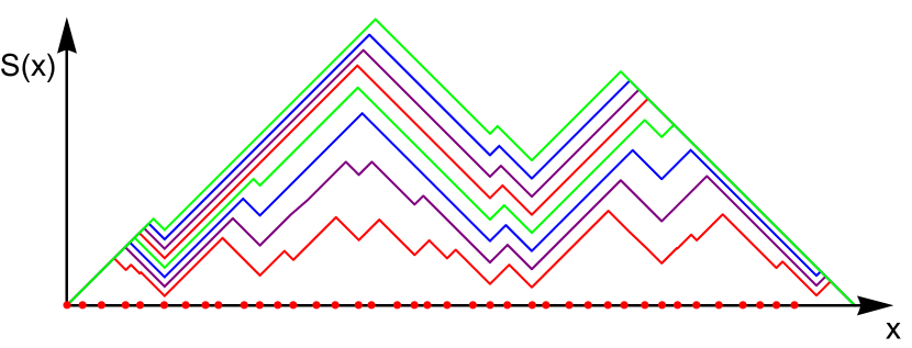
Fig. 1 shows growth according to the rule in Eq. 6. In the next section we will see how it emerges at large length and time scales from a semi-microscopic toy model.
A simple optimization argument tells us how scales with time if we start from a pure product state with . Let be the typical distance to the dominant weak link at time . The weakest link within this distance scale will have a rate of order , so the two terms in will scale as and respectively. Minimizing with respect to gives
| (7) |
The dynamical exponent sets the typical lengthscale for entanglement at time : for example the typical time for the entanglement profile to saturate in a finite system of size will be of order . It also governs the typical distance to the locally dominant weak link,
| (8) |
This is the lengthscale for the dynamical coarsening of the entanglement pattern visible in Fig. 1.
A key feature of Eq. 7 is that the entropy grows ‘sub-ballistically’ even for arbitrarily weak disorder: i.e. exceeds one even for arbitrarily large . This is despite the fact that operator growth is ballistic for large enough , as we will explain in Sec. III. Eq. 7 differs from earlier results which effectively assumed the timescale for entanglement saturation of a large chain was equal to a timescale associated with the weakest link in the chainVosk et al. (2015); Potter et al. (2015). These previous works took a viewpoint of the ‘spreading’ of entanglement, while we now argue that this process is more accurately viewed as the constrained local production of entanglement.
Since in Eq. 7 is the minimum of a set of uncorrelated random variables it is straightforward to find its full probability distribution in the limit of an infinite chain initiated in a pure product state. If the density of weak links is and the distribution of local rates is (2) at small , the cumulative probability distribution at long time is
| (9) |
with (restoring the equilibrium entropy density )
| (10) |
The surface growth picture is restricted to the entanglement across a single cut; to generalize to regions with multiple endpoints, or to periodic boundary conditions, we may use the ‘directed polymer’ description in Sec. II.2.
II.1 Random circuit model
Quantum circuit dynamics, with randomly chosen 2-site unitaries, capture many universal features of entanglement growth in translationally invariant systems Nahum et al. (2016). This setup is easily adapted to give a toy model for entanglement growth in the presence of weak links. This leads to a concrete surface growth problem defined on the lattice, from which the coarse-grained rule (6) can be seen to emerge in the scaling limit. This is not a derivation of the surface growth picture for isolated 1D systems with time-independent Hamiltonian or Floquet dynamics, whose microscopic dynamics are very different from the toy model; however it motivates the surface growth picture, some of whose predictions can subsequently be checked by other means.
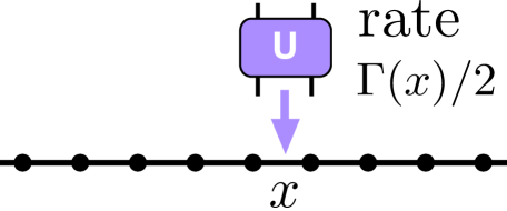
Consider a chain of ‘spins’, each with a large local Hilbert space dimension, . The chain is initially in an unentangled product state. Random 2-site unitaries are then applied to adjacent spins in a Poissonian fashion, at rates that depend on the bond (Fig. 4). These rates are distributed at small as in Eq. 2.
At large the dynamics of the entanglement across bond maps exactly to a classical surface growth model Nahum et al. (2016). We absorb a factor of into the definition of (by defining the von Neumann entropy using a logarithm base ). The entanglement then obeys a very simple dynamical growth rule: Each time a unitary is applied to bond , increases to the maximal value allowed by the general constraint that can exceed for the neighbouring bonds by at most . With this growth rule, the differences between adjacent heights are always at late times Nahum et al. (2016).
The resulting dynamics is microscopically stochastic. However we may neglect the noise-induced fluctuations, since they are negligible in the long-wavelength limit.
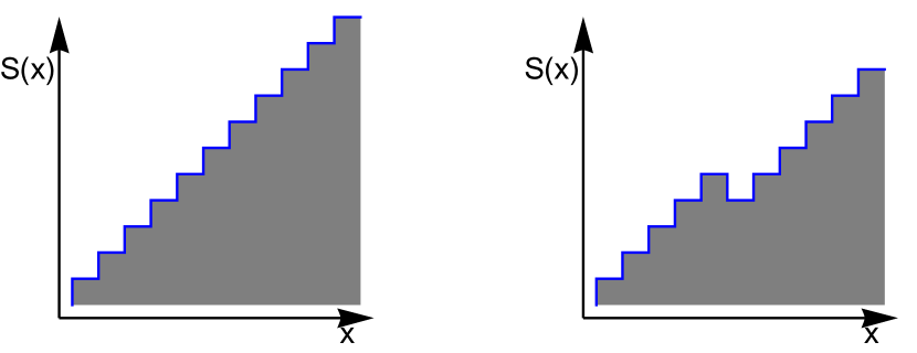
First take to be constant (no weak links), and consider the growth of a region whose coarse-grained slope is constant. If the surface is flat, , the growth rate is Meakin et al. (1986). The important regime for us will instead be where the slope is close to the maximal value of unity. Microscopically this means that the surface is close to the perfect staircase configuration shown in Fig. 3, Left. Note that the growth rate vanishes in this configuration. However when is slightly smaller than unity, there is a small density of ‘defects’ in the staircase, involving a local minimum of the height: see Fig. 3, Right. These defects allow growth. Each time a unitary hits a defect, the local height increases by two units. The coarse-grained growth rate is thus . The coarse-grained slope is given by , so
| (11) |
Note that, microscopically, each time a unitary hits a defect the defect moves up the staircase by one step, so defects run up the staircase at an average speed . The growth rate can be also be thought of as (twice) the ‘current’ of these defects.

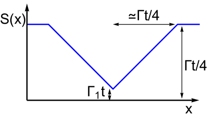
Next consider entanglement growth in a system with a single weak link at the origin, with rate . At a typical time the local configuration resembles Fig. 5, Left. Microscopically the weak bond is almost always a local minimum of the height profile. Unitaries are applied there at a rate , causing growth at rate . Each such event launches one defect up each staircase on the two sides of the weak link. The growth rate of the adjacent regions is therefore set by the growth rate at the weak link, . The coarse-grained slope of the adjacent regions is fixed using (11): . For small , the deviation of the slope from unity is small. Neglecting this deviation,
| (12) |
when the initial state is a pure product state. This profile is shown in Fig. 6, Left. The weak link influences a region of size on either side.
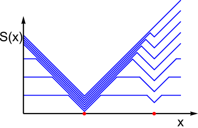
It is straightforward to generalize to multiple weak links. Consider two with rates and that are separated by a distance . (Fig. 6, Right.) We take . The regions of influence of the two weak links meet at a time , giving a profile with a central peak. The region of influence of the weaker link then gradually expands at the expense of the stronger link. At time the central peak hits the link with the rate and disappears. Subsequently the link with the larger rate has no effect on the coarse-grained configuration, being ‘dominated’ by the weaker link. (The link with rate does not affect the slope, or equivalently the density of defects, in this regime, except precisely at its location: the flow of defects is limited only by the slower rate .) Again we may write
| (13) |
The same logic extends to arbitrary numbers of weak links. The term can be dropped since at large times every point is within the domain of influence of some weak link. This gives Eq. 6.
We may also quantify the subleading corrections to Eq. 6: the average gradient of the straight sections111 For large the profile consists of staircases of typical length with almost-maximal coarse-grained . The minima between such staircases are weak links with typical strength (see above Eq. 7). The gradient at position is less than the maximum by . Summing this, the total height of the staircase is reduced from that of a perfect staircase by of order (note ) which gives the scaling in the text. is reduced from the maximal value of unity by an amount of order when and of order when . Since these corrections are indeed small.
II.2 ‘Minimal cut’ interpretation
There is a general relationship between surface growth in 1+1D and the statistical mechanics of a directed polymer in a two-dimensional environment Kardar et al. (1986). The results discussed above may also be understood in this language, and this allows them to be generalized to more complex geometries.
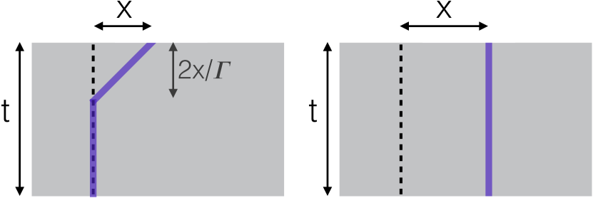
In the context of entanglement the directed polymer may be viewed as a coarse-grained ‘minimal cut’ through a unitary circuit representing the dynamical evolution Nahum et al. (2016). We briefly summarize the main features of this coarse grained picture as it applies to the random circuit model. In the present case, with weak links, we obtain a directed polymer subject to pinning by vertical defect lines Krug and Halpin-Healy (1993).
The entanglement is given by the ‘energy’ of a minimal–energy cut which splits the space-time slice into two disconnected pieces — see Fig. 7. (In this section we treat the time as a spatial dimension.) One endpoint of this cut must be at position on the top boundary, and the cut must disconnect the parts of the top boundary to the left and right of . In an infinite system this means that the other endpoint of the cut must be at the bottom boundary. In the absence of weak links, the minimal energy such cut is vertical, and the energy per unit height is (in the notation of Ref. Nahum et al. (2016) this is the entanglement rate ). In a finite system, the cut can terminate on the left- or right-hand spatial boundary.
To begin with it is sufficient to consider only horizontal and vertical cuts. The energy of a horizontal cut is equal to its extent in the direction. If we consider in a clean semi-infinite system with a boundary at position 0, the minimal cut is vertical and of energy for early times, while at late times the horizontal cut with energy is favourable; this gives .
A single weak link corresponds to a vertical defect line where the energy density per unit height is reduced and equal to . For large , it is worthwhile for the polymer to travel a large horizontal distance to take advantage of this favourable energy density. It must of course ‘pay’ in energy for the non-vertical section required to reach the defect. For a crude picture we can consider only horizontal and vertical segments; it is easy to see that in an infinite system we then recover Eq. 12.
In more detail, the energy of a segment of horizontal extent remains equal to even if the segment is at a finite angle to the horizontal, so long as this angle is small enough222This can be seen from the microscopic picture of the polymer as a ‘minimal cut’ through the large- unitary circuit. The energy of the polymer is equal to the number of bonds it cuts. A horizontal cut of length cuts bonds. This horizontal cut can be deformed to one with a finite coarse-grained slope, with the same energy, so long as the slope is (this is the typical vertical distance that the cut can travel before being blocked by a unitary). (this is true for slopes ). This means that the true minimal cut configuration for small is as shown in Fig. 7. This corresponds to taking subleading corrections in the slope of into account, and gives in agreement with the previous section.
This picture may be extended to multiple weak links. The typical transverse excursion for a given cut is of order , so much smaller than (Eq. 8). It may also be extended to a region with multiple endpoints. Consider the entanglement of a finite region of length in an infinite system. At early times the minimal cut configuration involves two disconnected cuts, giving an entanglement of order which is the sum of two independent random variables distributed as in Eq. 9. Once this becomes equal to , a configuration with a single horizontal cut becomes favourable.
III Operator spreading
Heisenberg time evolution will transform a local operator, for example the Pauli matrix located at the origin in a spin chain, into a complex object which acts nontrivially on many sites. The spatial extent of this growing operator may be quantified using the commutator with a local operator at site Lieb and Robinson (1972). In particular one can define the recently much-studied object Larkin and Ovchinnikov (1969); Kitaev (2014); Shenker and Stanford (2014a, b); Roberts et al. (2015); Maldacena et al. (2016); Aleiner et al. (2016); Patel and Sachdev (2017); Chowdhury and Swingle (2017); Patel et al. (2017); Stanford (2016); Banerjee and Altman (2017); Gu et al. (2016); Roberts and Swingle (2016); Huang et al. (2016); Fan et al. (2016); Chen (2016); Swingle and Chowdhury (2016); He and Lu (2016); Chen et al. (2016); Slagle et al. (2016); Roberts and Stanford (2015); Dóra and Moessner (2016); Bohrdt et al. (2016); Luitz and Lev (2017); Leviatan et al. (2017)
| (14) |
where is the density matrix at the appropriate temperature. Expanding the squared commutator gives the ‘out-of-time-order’ (OTO) correlator
| (15) |
is of order one in a spatial region whose size grows with , and vanishes far outside this region. In translationally invariant systems the size of the operator, as measured by , grows ballistically with a speed known as the butterfly speed.
Here we address the size and ‘shape’ of spreading operators in the thermal Griffiths phase; see Fig. 8. For simplicity we consider the case , but we do not expect this to change the basic results. We determine dynamical exponents and which give respectively the typical size of the operator at time and the typical size of its ‘front’ — the region in which is of order one, but smaller than the saturation value. The shape of the operator turns out to be qualitatively different for weak and strong disorder. For weak disorder : in this regime the front is much smaller than the ‘plateau’ region in which has saturated to its maximum value. Conversely for strong disorder , so that does not have a well-defined plateau when lengths are scaled by the spreading length.
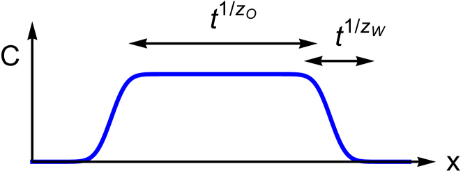
Our starting point is a picture for operator spreading in 1D systems developed on the basis of calculations in random circuits in Ref. Nahum et al. (2017) (see also parallel work which appeared recently von Keyserlingk et al. (2017)). It is shown there that for and for long times we may write (we switch to a continuum notation)
| (16) |
where is a conserved density
| (17) |
and where — in a random circuit without weak links — behaves essentially like the probability density of a random walker with a bias in favour of rightward steps. The average speed of the walker sets the butterfly velocity. For , the bulk of the density is within the range of integration in (16), yielding ; for the density is mostly outside the range of integration, giving . The transition region broadens diffusively, with width . This picture in terms of the density generalizes very naturally to the situation with weak links, where is no longer necessarily nonzero.
Let us briefly summarize the meaning of the density Nahum et al. (2017). First write the spreading operator at time in the basis of products of Pauli matrices,
| (18) |
Here is a string (product) of Pauli matrices at different sites. These strings satisfy
| (19) |
and since we have . The density is the ‘fraction’ of strings which end at position (a string ends at if is the rightmost site at which it acts nontrivially):
| (20) |
The density is evidently conserved and is normalized to one, , despite the fact that the number of distinct strings contributing to this density grows exponentially with time.
Consider for . Inserting the expression (18) shows that is
| (21) |
where the primed sum includes only those strings whose commutator with is nontrivial. Strings whose right endpoint is at a position to the left of cannot contribute to this sum, but an fraction of those whose right endpoint is to the right of do contribute. Specifically we expect333A given string can either have or at site (two of which commute with ), and we expect all options to be equally likely Nahum et al. (2017) deep in the interior of the operator. this fraction to be , giving (16). In a random circuit without weak links, may be argued to satisfy a noisy diffusion equation with bias Nahum et al. (2017).
This motivates the following picture for a system whose dynamics is deterministic but spatially random. We first consider the spreading of an operator through a single weak link, and then generalize to a Griffiths chain with many weak links.
III.1 Operator spreading across one weak link


Consider two regions in which operators spread at speed , separated by a weak link characterised by a very small rate . For simplicity we think of the weak link as a weak bond at position , and consider its effect on the rightward front of an operator which is initially localized in the leftward part of the system.
First, the density advances to the weak link, which we take to be located at position , reaching the weak link at time . We neglect the diffusive spreading in prior to passing through the weak link. It is easy to restore this effect in what follows by a more detailed treatment of biased diffusion on a chain with weak links, but it is not important for the scaling exponents below. The density then leaks through at a rate , so
| (22) |
where is the lattice site to the left of the weak link. The density on the other side of the weak link is
| (23) |
(Walkers hop across at rate , and are whisked away at speed .) Since we neglect spreading of within the homogeneous region, the density to the right of the weak link is related to the above by : for we have
| (24) |
At times (but small compared to , when diffusive spreading becomes comparable) the packet is of width and of height . See Fig. 9, Top.
III.2 Operator spreading across many weak links
To understand spreading across multiple weak links it is useful to think of each one as performing a linear transformation on the ‘wavepacket’ . We go into a frame moving at speed . The foregoing tells us that if the initial wavepacket is
| (25) |
then the new wavepacket is (we define ):
| (26) |
In other words, by linearity,
| (27) |
This transformation may be iterated.444E.g. for one choice of initial condition, iterating with the same value of gives (), which becomes Gaussian for large . It preserves the normalization of and it acts in a simple way on the mean and variance. If the th weak link encountered has strength ,
| (28) |
III.3 Operator spreading in the Griffiths phase
Next let us consider the leading edge of the commutator as it passes through a sequence of weak links , with a probability distribution . (We take the separation of the weak links to be unity.) There are three separate questions: (i) How far has the leading edge travelled at time ? (ii) What is the typical width of the leading edge after a time , within a given sample, i.e. for a given realization of the quenched disorder? (iii) How much variation in the position of the leading edge is there between different disorder realizations?
After traveling a distance the wavepacket has passed through weak links. From the formula for the mean, the position of the wavepacket is
| (29) |
where we have made the approximation that all parts of the wavepacket have passed through the same number of weak links. (This simplification does not change the scaling of , but must be considered more carefully for the fluctuations below.) The scaling of the sum in (29) depends on the value of . In the regime , the sum is proportional to the number of terms, whereas for it is dominated by the smallest , which is of order . This gives:
| (30) | |||||||
| (31) |
where we have introduced the dynamical exponent governing the size of a spreading operator.
Now let’s estimate the spreading of the wavepacket within a given sample. The variance formula (28) gives
| (32) |
This formula will give the correct scaling in the regime where all parts of the wavepacket have passed through links. This is the case for , where (32) gives a width much smaller than . Interestingly, there are two distinct behaviours within the regime: for the sum is of order , while for it is dominated by the minimal element:
| width | (33) | |||||||
| width | (34) |
When , naive application of the variance formula gives , showing that the approximation that all parts of the wavepacket have travelled through weak links breaks down. In this regime we expect simply that , i.e.
| width | (35) |
To see this, note that at time some of the wavepacket will have passed through the weakest nearby link, which is at distance and has rate , but some of the wavepacket will still be held up by the second weakest nearby link, which is an fraction of the distance away.
Putting these results together,
| width | (36) | |||||||
| width | (37) | |||||||
| width | (38) |
These formulas define a dynamical exponent governing the width of the front of a spreading operator.
So far we have considered the width within a given sample. Sample-to-sample variations in the front position are even more simply understood using (29). We find that in all regimes they scale with the same power of as the width of the front within a given realization.
The exponents above are written in terms of the parameter governing the distribution of weak link timescales. In using the same value of for operator spreading and for entanglement spreading, we are making the natural (but unproven) assumption that the timescales for entanglement growth and operator spreading are of the same order for a severe weak link.
There is a relationship between the growth of the second Renyi entropy and the spreading of the operators appearing in an expansion of the reduced density matrix, which has been used to give heuristic pictures for entanglement growth Ho and Abanin (2017); Mezei and Stanford (2016). Nevertheless the growth ‘speed’ associated with entanglement is in general smaller than that for the spreading of operators, even in clean systems Nahum et al. (2016); Mezei and Stanford (2016). The Griffiths phase is an extreme example, where the two lengthscales grow with different powers of time.
To summarize, operators have a well-defined front and a nonzero butterfly velocity only when . In all regimes the width of the front increases with time, and there is a change in the exponent governing this width at . The various dynamical exponents are summarized below in Table 1.
III.4 Operator entanglement
We may also consider the entanglement of a spreading operator, viewing the operator as a state in a “doubled” system Jonay and Huse . The growth of this operator entanglement within the region in between the two “fronts” of the spreading operator is governed by essentially the same physics as that governing the growth of the entanglement of states. Thus we expect the operator entanglement to grow with dynamic exponent . Since for all allowed finite within , the entanglement across the midpoint of a spreading operator is less than “volume-law” as long as it is spreading, where we call the distance between the two fronts the operator’s “volume”: . Interestingly, this exponent is non-monotonic. It is minimal at (assuming that timescales are characterized by a single exponent ), and the ‘volume law’ exponent of unity is recovered in both limits, and .
Once the operator reaches the ends of the chain it can then become volume-law entangled.
IV Conserved quantities
Here we revisit the dynamics of conserved quantities in the Griffiths phase, considered previously in Refs. Vosk et al. (2015); Potter et al. (2015); Agarwal et al. (2015), in order to compare with the spreading of operators and entanglement. We recover the dynamical exponent found previously for conserved quantities:
| (39) |
In writing (39) in terms of the exponent (Eq. 2) we have assumed that a weak link has a single associated timescale which governs both entanglement growth and ‘hopping’ of conserved quantities across the weak link. If there are cases where this assumption fails, a distinct exponent could appear in the formula (or even multiple s for different conserved quantities). It is natural to expect at least that : the ‘hopping’ of (say) a conserved charge across the weak link will generically induce entanglement, so the rate for entanglement production should not be parametrically smaller than that for conserved quantities.
Since the system locally looks thermal at late times, we may treat the dynamics of conserved quantities as a classical random walk — say on a 1D lattice, in continuous time — which is ‘bottlenecked’ by weak links. We treat the weak links as bonds where the hopping rate is small. This setup preserves detailed balance.
For weak disorder, the dynamics is diffusive. To see when diffusive scaling breaks down, consider two adjacent weak links with . Their interior defines a box of typical size
| (40) |
Now compare the time for a diffusing particle to cross this box, , with the time for which the particle is detained by a single weak link of strength . Once the walker reaches the weak link it must revisit it times before it succeeds in hopping across. By standard diffusive scaling, the time required for this number of revisits is . When we have , and we expect diffusive scaling to be stable. On the other hand when the two weak links trap the walker inside the box for much longer than . In this regime will be of the same order as the time required to explore the box ‘ergodically’. The rate to cross one of the weak links is then the product of the fraction of the time spent adjacent to the weak link, namely , with the rate at the weak link. The typical time required to escape the box is therefore
| (41) |
This gives the dynamical exponent quoted above. This exponent agrees with the random walk model of Ref. Potter et al. (2015), but the behaviour of trajectories is different.555In the regime a walker takes a time of order to traverse a sample of size , where is the typical size of the weakest link in the sample. In the above model this timescale is associated with trajectories that traverse the weak link times, whereas in the model of Ref. Potter et al. (2015) it is associated with trajectories which traverse the weak link times.
The transition between diffusive and subdiffusive behaviour has been observed numerically in a disordered Heisenberg chain Žnidarič et al. (2016); see also Refs. Luitz et al. (2016); Agarwal et al. (2015); Bar Lev et al. (2015); Khait et al. (2016).
If a quantum quench starts from a sufficiently inhomogeneous initial state, the relaxation of conserved quantities will affect the growth of entanglement. An extreme example is a 1D spin chain, with conserved , which starts in a domain wall state with fully polarized up spins on the left and fully polarized down spins on the right. Since a polarized region has trivial dynamics, entanglement can only be generated in the growing central region where the polarization has been destroyed. For an initial state with only short-range correlated randomness in conserved quantities, the local expectation value of the conserved quantity will relax to equilibrium with fluctuations of order . These fluctuations will lead to fluctuations in the local entangling rates for the weak links, but these will be negligible at late times.
V Dynamical exponent summary
The dynamical exponents we have found are summarized in Table. 1, under the assumption (see caveats in Secs. III.3, IV) that the long timescales characterizing a weak link are distributed with the same power law.
VI Bounding entanglement growth across a Griffiths region
In previous sections we assumed that a Griffiths region could be characterised by a local entanglement growth rate, , which vanishes as the region becomes large. Here we show analytically that the rate for entanglement growth across a Griffiths region is exponentially slow when the length of the Griffiths region is large.
We will start by considering a trivial kind of weak link — a weak bond in a spin chain. For this simple case, a standard rigorous result provides a bound on the entanglement growth rate. A Griffiths region is more complicated: although it acts as a weak link in a coarse-grained sense, it is not equivalent to a simple weak bond, and the degrees of freedom within the Griffiths region are strongly coupled. Nevertheless we show below that the bound can be extended — nonrigorously — to this case by making use of the ‘l-bit’ picture for many-body localized systems Huse et al. (2014); Serbyn et al. (2013b).
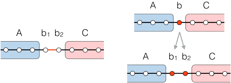
First consider a spin chain in which one bond has a very small coupling. Label the degrees of freedom as in Fig. 10, Left. and denote the spins to the left and right of the weak bond respectively, and and contain the other spins on the left and the right respectively. The Hamiltonian may be written
| (42) |
reflecting the fact that the two sides are coupled only via spins and . For example, for an infinite chain with Ising interactions and longitudinal and transverse fields, we would have
| (43) | ||||
| (44) | ||||
| (45) |
with . This is a weak link of a simple kind: the systems and are coupled only by a small term in the Hamiltonian. In this simple situation there is a rigorous bound on the rate at which entanglement can be generated across the weak link Van Acoleyen et al. (2013); Audenaert (2014); Bravyi (2007). This bound states that in a pure state
| (46) |
Here is a numerical constant given in Van Acoleyen et al. (2013); is the smaller of the Hilbert space dimensions of and , here given by . Most importantly, is the magnitude of the largest eigenvalue of , here equal to .
For small the physical rate of entanglement growth (i.e. in a typical state) may be much smaller than the rigorous upper bound (46). Indeed, numerically we find that in a Floquet Ising spin chain the von Neumann entropy growth rate is of order
| (47) |
rather than of order , see Sec. VII. But for our purposes in this section the upper bound (46) will suffice.
Microscopically, a Griffiths region does not consist of weakly-coupled degrees of freedom, so we cannot immediately apply (46). A better cartoon is that the Griffiths region consists of ‘slow’ degrees of freedom. To see this, recall that deep in the MBL phase the Hamiltonian may be formulated in terms of ‘l-bits’ — dressed spin variables whose -components are strictly conserved Huse et al. (2014); Serbyn et al. (2013b). This picture is also a useful starting point for considering strongly disordered regions which locally resemble the MBL phase. Since these regions are finite, the dressed spin variables are not strictly conserved, but are instead ‘slow’.
We can learn how to treat such slow degrees of freedom in the context of a toy model, where the Griffiths region is replaced by a single central spin whose -component is almost conserved. See Fig. 10, right. We label the left and right regions by and respectively, and the central slow spin by . We denote the Pauli operators for the slow spin by , , , and take a Hamiltonian whose terms all commute with :
| (48) |
Here the notation means that this term acts on the central spin only via its operator; it can act arbitrarily on the spins in . For concreteness we take the weak term which breaks conservation of to be a transverse field.
It is easy to find an example showing that the instantaneous rate of entanglement growth between and the rest, , can be .666Take to be empty and to consist of a single spin, take to be an Ising coupling, and take the initial state to have both spins polarized in the direction. However the time-averaged rate is small when is small. To see this we relate the physical system to a reference system in which the spin is replaced with two spins. There is a mapping from the Hilbert space of into that of given by
| (49) |
in the basis. This mapping commutes with the time evolution if we choose the following Hamiltonian for the reference system:
| (50) |
where is simply with replaced by . Further, if two states and are related by the mapping, they yield the same density matrix on . Therefore we are guaranteed that
| (51) |
at all times.
Since the weak field has now become a weak interaction between and , we can use Eq. 46 to bound the change in the entanglement between and :
| (52) |
Of course is not meaningful in the physical system. But subadditivity of the von Neumann entropy, together with (51), guarantees that it is close to the quantity of interest: . This gives the desired result
| (53) |
We see that at long times the time-averaged is at most of order , and that the coefficient remains of even if the size of or diverges. (See Sec. VII for a numerical analysis of this problem in a Floquet spin chain, showing that the growth rate is even smaller than the maximum allowed by this bound.)
Finally we turn to a spin chain with subsystems , where is a Griffiths region consisting of a large number of consecutive spins. We will consider a strongly disordered Griffiths region which locally resembles the fully many body localized phase. Write the Hamiltonian as
| (54) |
where and each act on a single bond. Now we make use of the l-bit picture for the MBL phase Huse et al. (2014); Serbyn et al. (2013b). We expect that a unitary transformation on can reduce its Hamiltonian to a form which only depends on the operators for spins ,
| (55) |
where the couplings decay exponentially with distance, and where the unitary transformation preserves the locality of operators up to exponential tails. For the purposes of entanglement growth we can work with instead of , since only introduces entanglement. is of the form
| (56) |
If , where , are the boundary spins in and respectively,
| (57) |
Now we split the Griffiths region into the left-hand, central and right-hand regions, , , and , of length each, and apply the duplication trick to to give a system
| (58) |
We now consider generation of entanglement across the cut . The terms in and act only within or respectively and can be neglected. Next we have the terms coming from . These act on all the s in . We have some freedom in how we represent these terms, since any in can be represented either by a in or by the corresponding in . Using this freedom, any term in which does not act on both and may be represented with a term which does not cross the cut . The largest remaining terms from , which act on both and , are of magnitude . These terms typically act on spins in region but only spins in and , so can be represented by terms involving only spins on one side of the cut and on the other. Finally we have the terms from and which couple across the boundary of the Griffiths region. After the unitary transformation, couples the boundary spin in region to all of the -bits in the Griffiths regions, with exponentially decaying couplings. Terms in which is coupled to the leftmost spins in region are of size . A term like , where is a site in region , becomes a coupling involving the corresponding sites in both and . Again these terms involve spins on one side of the cut and on the other.
Altogether, the strongest terms in the Hamiltonian which couple across the cut have size and involve spins.777These terms can be split into two groups, each of which acts on only spins from one side. Since (46) can be applied to each group separately and the results added, the appropriate factor (46) is rather than . In any case this polynomial correction is negligible in comparison to the error in estimating the coefficient in the exponential. For a nonrigorous application of the bound (46), we must estimate the norm of the entangling Hamiltonian. This may be larger than by an exponentially large combinatorial factor, since the number of terms is large. We take the region to be sufficiently strongly disordered (i.e. , where is an order one constant) that the exponential decay of the couplings wins, giving
| (59) |
for some which does not depend on . The difference between and the physically meaningful entropy (or is , and is unimportant at long times.
This shows that the entanglement growth rate across a strongly disordered Griffiths region is exponentially small in the size of the region, regardless of the size of the complete chain. (Assumptions made in previous work are equivalent to taking the entanglement growth rate to grow with the size of the adjacent regions, which we see is not the case.) This is enough to show that there is a power law distribution of local rates. In turn this suffices to prove that grows subballistically, by the logic in Sec. II. We focussed on strongly disordered regions with , while in practise the prevalent weak links with a given may be less strongly disordered. However this will only decrease the value of the exponent .
VII Entangling across a weak link: numerics

We now present a numerical study of entanglement growth across a microscopic weak link. The setup for the numerical simulation is a spin- chain of length , shown schematically in Fig. 11. We use Floquet dynamics considered previously in Ref. Zhang et al., 2015: an Ising spin chain with longitudinal and transverse fields. This system has been shown to thermalize rapidly in the absence of a weak link. A simplifying feature of the Floquet case is that energy is not conserved Zhang et al. (2015). The time evolution is implemented using the online package ITensor ITe .
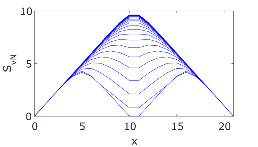
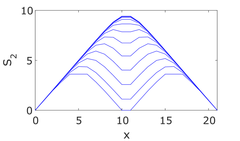
The weak link we consider is formed by the spin at the central site, whose -component is almost conserved. The commutator of this operator with the one-step time evolution operator is of order , where will be taken to be small. As discussed in Sec. VI, this is a toy model for a Griffiths region: the central spin is an ‘almost’ -bit, whereas all other spins are strongly non-conserved under the evolution. The slow spin bottlenecks the growth of entanglement between the rapidly thermalizing regions surrounding it. We focus on the dynamics of the Renyi entropies (including the von Neumman entropy )
| (60) |
across the bond connecting the spin at site to the nearly conserved spin ( and the regions and are defined in Fig. 11).
Here we will give results only for the model with a slow spin, but we have also simulated a spin chain with a weak bond. As might be expected from the mapping between a slow spin and a weak link in Sec. VI, the results are extremely similar Nahum et al. .
Our main goal will be to validate two key elements of the picture for entanglement growth discussed above. Firstly, that the entanglement growth rate in the vicinity of a weak link, , can be characterized by a local rate which is independent of the size of the surrounding regions. Secondly, that in the scaling limit the growth of entanglement entropy is captured by the simple scaling forms discussed in Sec. II. For the present case, the relevant scaling form, if we start from a product state, is:
| (61) |
where is the location of the weak link. If we start from a state in which the two subsystems are separately fully entangled,
| (62) |
In particular, either of these forms implies that for large and , the entanglement at the location of the weak link has the simple piecewise linear scaling form
| (63) |
Although simple, these scaling forms are not a priori obvious: they are nontrivial predictions about the universal physics stemming from the results of this paper.
There are many other natural questions about how weakly coupled systems get entangled over time, but we defer these to a future publication Nahum et al. .
We now give details of the numerical simulation. We use a Floquet time evolution operator
| (64) |
which includes half a period of evolution with the Ising interactions and longitudinal fields,
| (65) |
preceded by half a period of evolution with the transverse fields,
| (66) |
Note that the transverse field on the central spin is weakened by a (variable) factor . The other couplings are fixed at the values , , , which were shown in Ref. Zhang et al., 2015 to yield rapid thermalization.
We start from the product state in the basis. But before beginning the entangling dynamics, we evolve the left and right subsystems separately, i.e. with , for a time to ensure that they are separately strongly entangled. In the simulations we have used , however, we note that our results depend very weakly on . The state at time is therefore defined to be
| (67) |
Note that the entanglement between and is zero when . In Fig. 12 we plot a typical spatial dependence of for a system of size and for successive times starting from . Fig. 13 shows the same for .
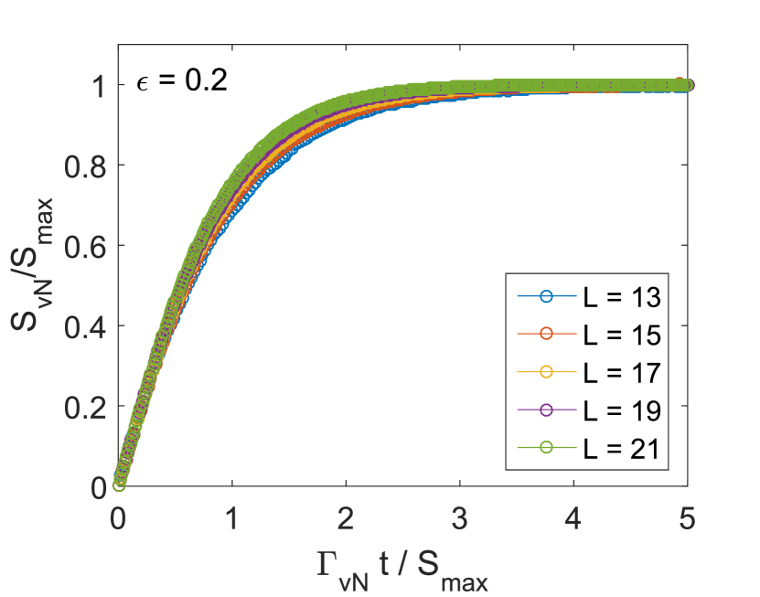
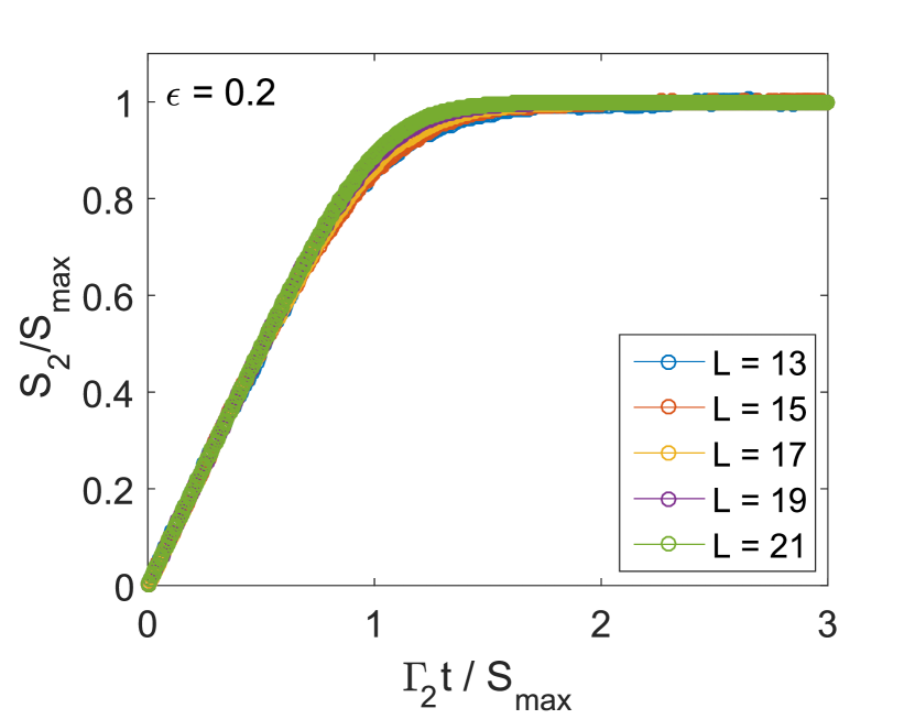
Let us now examine the validity of the scaling forms. In Fig. 14 we plot the the von Neumann and second Renyi entropies, rescaled by their asymptotic late time values, against the rescaled time variable . Here is the growth rate of obtained by fitting the linear growth near for . is the value of the entropy as , which is determined numerically and which depends on and . We note that in the case of the von Neumann entropy converges very quickly with increasing to the prediction of Ref. Page, 1993 for a random state.
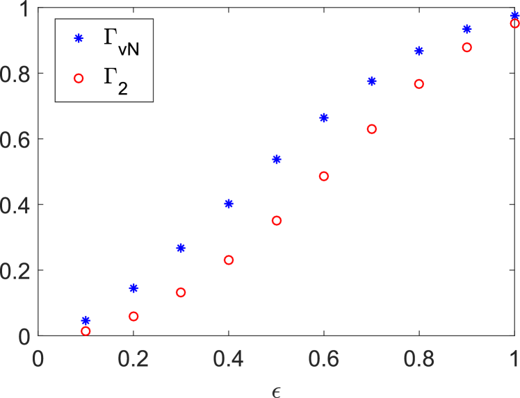
It is clear from Fig. 14 that the early time growth rate, , is independent of the length of the system. This is consistent with our coarse-grained picture. By numerically fitting the data we find that for small the growth rates are given by
| (68) |
where and are –independent constants. The rates for larger values of are shown in Fig. 15. This confirms that indeed the growth rate is small in and that a nearly conserved quantity causes a bottleneck for entanglement growth. Note that for small the growth rate is parametrically smaller than the rigorous upper bound in Sec. VI. Interestingly, Fig. 15 suggests that for (the homogeneous case) the growth rates for and may be equal.
We also find that the transition from linear growth to saturation becomes sharper with increasing , consistent with the expected scaling form Eq. (63). This is much clearer for the second and higher Renyi entropies (Fig. 14). For the von Neumann entropy a more careful finite size analysis is required, which we give below.
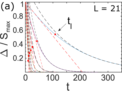
For translationally-invariant Floquet systems with no conserved quantities, the late time saturation of the entropy has been found to be exponential Zhang et al. (2015). We also obtain a good fit at late times with
| (69) |
where the parameters and of the fit are extracted separately for each and . We find that at small the saturation rate behaves as
| (70) |
The time scale for saturation is of order .
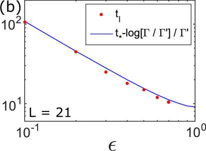
Assume that there is a simple crossover between linear and exponential behaviour at a time . Matching and at this time gives the following gluing conditions:
| (71) |
which means that
| (72) |
In Fig. 16 we test the assumption underlying the previous. In the first panel we present the linear (red dashed lines) and exponential (black dashed lines) fits to . The red dots are crossover times between these two behaviors, determined by eye. In the second panel we compare these crossover times with the prediction in Eq. (71), finding good agreement.
The previous equation shows that the departure from linear behaviour occurs when the entropy is within
| (73) |
bits of its maximum. The behaviour for the von Neumann entropy indicates that the finite-size rounding is more severe for weaker weak links; this conforms with what we find numerically. For the higher Renyi entropies this logarithmic factor is absent, as a result of Eq. 68. Since is independent of , the above confirms the scaling form Eq. 63 for a system of size with a weak link whose strength is fixed as . (The deviation from linearity for the last bits of entanglement is also negligible if we take to scale as a negative power of , which is the natural scaling in the Griffiths regime.)
Note that if the relative logarithmic factor in the growth rates for and (Eq. 68) also applies for coarse-grained weak links, then the von Neumman entropy in the Griffiths phase will exceed the higher Renyi entropies by a factor of order at late times (since the weak links that are relevant at time have strength ).
We have confirmed the two key assumptions: is independent of , and the scaling form Eq. (6) is indeed obtained in the large limit for a microscopic weak link. If we allow ourselves to extrapolate the above results to Griffiths regions (coarse-grained weak links), these conclusions support the scaling forms derived from the surface growth picture.
VIII Summary
We have examined the dynamics of isolated one-dimensional quantum systems that thermalize, but have a distribution of weak links produced by quenched randomness. This occurs in systems which sustain (but which are outside) the many-body-localized (MBL) phase, due to Griffiths regions that are locally in this phase. We developed coarse-grained pictures for the production of entanglement and the spreading of operators and of conserved densities.
We found that such systems have multiple dynamic length scales that diverge with different powers of the time. These length scales are for: the growth of entanglement, the spreading of conserved densities, the spreading of initially local operators, and the width of the ‘front’ of a spreading operator. Contrary to systems without quenched disorder, the process of entanglement saturation (either for states or operators) is always parametrically slower than the spreading of operators as measured by the norm of their commutator with a local operator or by the out-of-time-order correlator.
We also examined the exchange of quantum information between two clean systems coupled by a single weak link, giving universal scaling forms for the growth of entanglement and the spreading of operators from one system into the other.
Various questions remain for the future. It has been suggested on the basis of simulations Lev et al. (2017) that sub-ballistic entanglement growth may occur in the thermal phase of 1D chains with quasiperiodic detuning rather than disorder. The relation of such systems to rare-region physics remains to be understood.
The pictures described here are set up to deal with dynamics in the thermal phase. It would be interesting to understand the crossover effects at the MBL phase transition Vosk et al. (2015); Potter et al. (2015); Khemani et al. (2017) in more detail. It may also be interesting to consider a coarse-grained treatment of the network of locally thermal Griffiths regions in the MBL phase. In higher dimensions, such rare regions have been argued to destabilize the MBL phase De Roeck and Huveneers (2017); De Roeck and Imbrie (2017).
Acknowledgements.
We thank S. Gopalakrishnan, J. Haah, C. Jonay, and S. Vijay for collaboration on related work. AN acknowledges support from the Gordon and Betty Moore Foundation under the EPiQS initiative (grant No. GBMF4303) and from EPSRC Grant No. EP/N028678/1. JR acknowledges a fellowship from the Gordon and Betty Moore Foundation under the EPiQs initiative (grant No. GBMF4303).References
- Calabrese and Cardy (2005) P. Calabrese and J. Cardy, “Evolution of entanglement entropy in one-dimensional systems,” J. Stat. Mech. 0504, P04010 (2005).
- Chiara et al. (2006) Gabriele De Chiara, Simone Montangero, Pasquale Calabrese, and Rosario Fazio, “Entanglement entropy dynamics of heisenberg chains,” Journal of Statistical Mechanics: Theory and Experiment 2006, P03001 (2006).
- Bardarson et al. (2012) Jens H. Bardarson, Frank Pollmann, and Joel E. Moore, “Unbounded growth of entanglement in models of many-body localization,” Phys. Rev. Lett. 109, 017202 (2012).
- Kim and Huse (2013) H. Kim and D. A. Huse, “Ballistic spreading of entanglement in a diffusive nonintegrable system,” Phys. Rev. Lett. 111, 127205 (2013).
- Nahum et al. (2016) Adam Nahum, Jonathan Ruhman, Sagar Vijay, and Jeongwan Haah, “Quantum entanglement growth under random unitary dynamics,” arXiv preprint arXiv:1608.06950 (2016).
- Nandkishore and Huse (2015) Rahul Nandkishore and David A Huse, “Many-body localization and thermalization in quantum statistical mechanics,” Annu. Rev. Condens. Matter Phys. 6, 15–38 (2015).
- Lieb and Robinson (1972) E. H. Lieb and D. W. Robinson, “The finite group velocity of quantum spin systems,” Commun. Math. Phys. 28, 251 (1972).
- Roberts et al. (2015) Daniel A. Roberts, Douglas Stanford, and Leonard Susskind, “Localized shocks,” Journal of High Energy Physics 2015, 51 (2015).
- Žnidarič et al. (2008) Marko Žnidarič, Tomaž Prosen, and Peter Prelovšek, “Many-body localization in the heisenberg magnet in a random field,” Phys. Rev. B 77, 064426 (2008).
- Serbyn et al. (2013a) Maksym Serbyn, Z. Papić, and Dmitry A. Abanin, “Universal slow growth of entanglement in interacting strongly disordered systems,” Phys. Rev. Lett. 110, 260601 (2013a).
- Huse et al. (2014) David A. Huse, Rahul Nandkishore, and Vadim Oganesyan, “Phenomenology of fully many-body-localized systems,” Phys. Rev. B 90, 174202 (2014).
- Huang et al. (2016) Y. Huang, Y.-L. Zhang, and X. Chen, “Out-of-time-ordered correlators in many-body localized systems,” ArXiv e-prints (2016), arXiv:1608.01091 [cond-mat.dis-nn] .
- Fan et al. (2016) R. Fan, P. Zhang, H. Shen, and H. Zhai, “Out-of-Time-Order Correlation for Many-Body Localization,” ArXiv e-prints (2016), arXiv:1608.01914 [cond-mat.quant-gas] .
- Chen (2016) Y. Chen, “Universal Logarithmic Scrambling in Many Body Localization,” ArXiv e-prints (2016), arXiv:1608.02765 [cond-mat.dis-nn] .
- Swingle and Chowdhury (2016) B. Swingle and D. Chowdhury, “Slow scrambling in disordered quantum systems,” ArXiv e-prints (2016), arXiv:1608.03280 [cond-mat.str-el] .
- He and Lu (2016) R.-Q. He and Z.-Y. Lu, “Characterizing Many-Body Localization by Out-of-Time-Ordered Correlation,” ArXiv e-prints (2016), arXiv:1608.03586 [cond-mat.dis-nn] .
- Chen et al. (2016) Xiao Chen, Tianci Zhou, David A. Huse, and Eduardo Fradkin, “Out-of-time-order correlations in many-body localized and thermal phases,” Annalen der Physik , 1600332–n/a (2016), 1600332.
- Slagle et al. (2016) K. Slagle, Z. Bi, Y.-Z. You, and C. Xu, “Out-of-Time-Order Correlation in Marginal Many-Body Localized Systems,” ArXiv e-prints (2016), arXiv:1611.04058 [cond-mat.str-el] .
- Vosk et al. (2015) Ronen Vosk, David A. Huse, and Ehud Altman, “Theory of the many-body localization transition in one-dimensional systems,” Phys. Rev. X 5, 031032 (2015).
- Potter et al. (2015) Andrew C. Potter, Romain Vasseur, and S. A. Parameswaran, “Universal properties of many-body delocalization transitions,” Phys. Rev. X 5, 031033 (2015).
- Agarwal et al. (2015) Kartiek Agarwal, Sarang Gopalakrishnan, Michael Knap, Markus Müller, and Eugene Demler, “Anomalous diffusion and griffiths effects near the many-body localization transition,” Phys. Rev. Lett. 114, 160401 (2015).
- Bar Lev et al. (2015) Yevgeny Bar Lev, Guy Cohen, and David R. Reichman, “Absence of diffusion in an interacting system of spinless fermions on a one-dimensional disordered lattice,” Phys. Rev. Lett. 114, 100601 (2015).
- Luitz et al. (2016) David J. Luitz, Nicolas Laflorencie, and Fabien Alet, “Extended slow dynamical regime close to the many-body localization transition,” Phys. Rev. B 93, 060201 (2016).
- Khait et al. (2016) I. Khait, S. Gazit, N. Y. Yao, and A. Auerbach, “Spin transport of weakly disordered Heisenberg chain at infinite temperature,” Phys. Rev. B 93, 224205 (2016), arXiv:1603.06588 [cond-mat.dis-nn] .
- Žnidarič et al. (2016) Marko Žnidarič, Antonello Scardicchio, and Vipin Kerala Varma, “Diffusive and subdiffusive spin transport in the ergodic phase of a many-body localizable system,” Phys. Rev. Lett. 117, 040601 (2016).
- Lüschen et al. (2016) Henrik P Lüschen, Pranjal Bordia, Sebastian Scherg, Fabien Alet, Ehud Altman, Ulrich Schneider, and Immanuel Bloch, “Evidence for griffiths-type dynamics near the many-body localization transition in quasi-periodic systems,” arXiv preprint arXiv:1612.07173 (2016).
- Luitz and Lev (2017) David J Luitz and Yevgeny Bar Lev, “Information propagation in isolated quantum systems,” arXiv preprint arXiv:1702.03929 (2017).
- Chandran et al. (2014) Anushya Chandran, Vedika Khemani, C. R. Laumann, and S. L. Sondhi, “Many-body localization and symmetry-protected topological order,” Phys. Rev. B 89, 144201 (2014).
- Potter and Vasseur (2016) Andrew C. Potter and Romain Vasseur, “Symmetry constraints on many-body localization,” Phys. Rev. B 94, 224206 (2016).
- Protopopov et al. (2016) I. V. Protopopov, W. W. Ho, and D. A. Abanin, “The effect of symmetry on many-body localization and thermalization,” ArXiv e-prints (2016), arXiv:1612.01208 [cond-mat.dis-nn] .
- Nahum et al. (2017) A. Nahum, S. Vijay, and J. Haah, “Operator spreading in random unitary circuits,” ArXiv preprints ArXiv:1705.08975 (2017).
- von Keyserlingk et al. (2017) C. W. von Keyserlingk, T. Rakovszky, F. Pollmann, and S. L. Sondhi, “Operator hydrodynamics, OTOCs, and entanglement growth in systems without conservation laws,” ArXiv preprints ArXiv:1705.08910 (2017).
- Page (1993) D. N. Page, “Average entropy of a subsystem,” Phys. Rev. Lett. 71, 1291–1294 (1993).
- Meakin et al. (1986) P. Meakin, P. Ramanlal, L. M. Sander, and R. C. Ball, “Ballistic deposition on surfaces,” Phys. Rev. A 34, 5091–5103 (1986).
- Kardar et al. (1986) M. Kardar, G. Parisi, and Y-C. Zhang, “Dynamic scaling of growing interfaces,” Phys. Rev. Lett. 56, 889–892 (1986).
- Krug and Halpin-Healy (1993) Joachim Krug and Timothy Halpin-Healy, “Directed polymers in the presence of columnar disorder,” Journal de Physique I 3, 2179–2198 (1993).
- Larkin and Ovchinnikov (1969) AI Larkin and Yu N Ovchinnikov, “Quasiclassical method in the theory of superconductivity,” Sov Phys JETP 28, 1200–1205 (1969).
- Kitaev (2014) A. Kitaev, “Hidden correlations in the hawking radiation and thermal noise,” in Talk given at the Fundamental Physics Prize Symposium (2014).
- Shenker and Stanford (2014a) Stephen H. Shenker and Douglas Stanford, “Black holes and the butterfly effect,” Journal of High Energy Physics 2014, 67 (2014a).
- Shenker and Stanford (2014b) Stephen H. Shenker and Douglas Stanford, “Multiple shocks,” Journal of High Energy Physics 2014, 46 (2014b).
- Maldacena et al. (2016) Juan Maldacena, Stephen H. Shenker, and Douglas Stanford, “A bound on chaos,” Journal of High Energy Physics 2016, 106 (2016).
- Aleiner et al. (2016) Igor L. Aleiner, Lara Faoro, and Lev B. Ioffe, “Microscopic model of quantum butterfly effect: Out-of-time-order correlators and traveling combustion waves,” Annals of Physics 375, 378 – 406 (2016).
- Patel and Sachdev (2017) Aavishkar A. Patel and Subir Sachdev, “Quantum chaos on a critical fermi surface,” Proceedings of the National Academy of Sciences 114, 1844–1849 (2017), http://www.pnas.org/content/114/8/1844.full.pdf .
- Chowdhury and Swingle (2017) Debanjan Chowdhury and Brian Swingle, “Onset of many-body chaos in the model,” arXiv preprint arXiv:1703.02545 (2017).
- Patel et al. (2017) Aavishkar A Patel, Debanjan Chowdhury, Subir Sachdev, and Brian Swingle, “Quantum butterfly effect in weakly interacting diffusive metals,” arXiv preprint arXiv:1703.07353 (2017).
- Stanford (2016) Douglas Stanford, “Many-body chaos at weak coupling,” Journal of High Energy Physics 2016, 9 (2016).
- Banerjee and Altman (2017) Sumilan Banerjee and Ehud Altman, “Solvable model for a dynamical quantum phase transition from fast to slow scrambling,” Phys. Rev. B 95, 134302 (2017).
- Gu et al. (2016) Yingfei Gu, Xiao-Liang Qi, and Douglas Stanford, “Local criticality, diffusion and chaos in generalized sachdev-ye-kitaev models,” arXiv preprint arXiv:1609.07832 (2016).
- Roberts and Swingle (2016) Daniel A Roberts and Brian Swingle, “Lieb-robinson bound and the butterfly effect in quantum field theories,” Physical Review Letters 117, 091602 (2016).
- Roberts and Stanford (2015) Daniel A Roberts and Douglas Stanford, “Diagnosing chaos using four-point functions in two-dimensional conformal field theory,” Physical review letters 115, 131603 (2015).
- Dóra and Moessner (2016) Balázs Dóra and Roderich Moessner, “Out-of-time-ordered density correlators in luttinger liquids,” arXiv preprint arXiv:1612.00614 (2016).
- Bohrdt et al. (2016) A Bohrdt, CB Mendl, M Endres, and M Knap, “Scrambling and thermalization in a diffusive quantum many-body system,” arXiv preprint arXiv:1612.02434 (2016).
- Leviatan et al. (2017) Eyal Leviatan, Frank Pollmann, Jens H Bardarson, and Ehud Altman, “Quantum thermalization dynamics with matrix-product states,” arXiv preprint arXiv:1702.08894 (2017).
- Ho and Abanin (2017) Wen Wei Ho and Dmitry A Abanin, “Entanglement dynamics in quantum many-body systems,” Physical Review B 95, 094302 (2017).
- Mezei and Stanford (2016) Márk Mezei and Douglas Stanford, “On entanglement spreading in chaotic systems,” arXiv preprint arXiv:1608.05101 (2016).
- (56) C. Jonay and D. A. Huse, To appear .
- Serbyn et al. (2013b) Maksym Serbyn, Z. Papić, and Dmitry A. Abanin, “Local conservation laws and the structure of the many-body localized states,” Phys. Rev. Lett. 111, 127201 (2013b).
- Van Acoleyen et al. (2013) Karel Van Acoleyen, Michaël Mariën, and Frank Verstraete, “Entanglement rates and area laws,” Phys. Rev. Lett. 111, 170501 (2013).
- Audenaert (2014) Koenraad M. R. Audenaert, “Quantum skew divergence,” Journal of Mathematical Physics 55, 112202 (2014), http://dx.doi.org/10.1063/1.4901039 .
- Bravyi (2007) Sergey Bravyi, “Upper bounds on entangling rates of bipartite hamiltonians,” Phys. Rev. A 76, 052319 (2007).
- Zhang et al. (2015) Liangsheng Zhang, Hyungwon Kim, and David A Huse, “Thermalization of entanglement,” Physical Review E 91, 062128 (2015).
- (62) “ITensor,” http://itensor.org.
- (63) A. Nahum, J. Ruhman, and D. A. Huse, To appear .
- Lev et al. (2017) Yevgeny Bar Lev, Dante M Kennes, Christian Klöckner, David R Reichman, and Christoph Karrasch, “Transport in quasiperiodic interacting systems: from superdiffusion to subdiffusion,” arXiv preprint arXiv:1702.04349 (2017).
- Khemani et al. (2017) Vedika Khemani, S. P. Lim, D. N. Sheng, and David A. Huse, “Critical properties of the many-body localization transition,” Phys. Rev. X 7, 021013 (2017).
- De Roeck and Huveneers (2017) Wojciech De Roeck and François Huveneers, “Stability and instability towards delocalization in many-body localization systems,” Physical Review B 95, 155129 (2017).
- De Roeck and Imbrie (2017) Wojciech De Roeck and John Z Imbrie, “Many-body localization: Stability and instability,” arXiv preprint arXiv:1705.00756 (2017).