Bayesian modelling of uncertainties of Monte Carlo radiative-transfer simulations

Abstract

One of the big challenges in astrophysics is the comparison of complex simulations to observations. As many codes do not directly generate observables (e.g. hydrodynamic simulations), the last step in the modelling process is often a radiative-transfer treatment. For this step, the community relies increasingly on Monte Carlo radiative transfer due to the ease of implementation and scalability with computing power. We consider simulations in which the number of photon packets is Poisson distributed, while the weight assigned to a single photon packet follows any distribution of choice. We show how to estimate the statistical uncertainty of the sum of weights in each bin from the output of a single radiative-transfer simulation. Our Bayesian approach produces a posterior distribution that is valid for any number of packets in a bin, even zero packets, and is easy to implement in practice. Our analytic results for large number of packets show that we generalise existing methods that are valid only in limiting cases. The statistical problem considered here appears in identical form in a wide range of Monte Carlo simulations including particle physics and importance sampling. It is particularly powerful in extracting information when the available data are sparse or quantities are small.

1 Introduction

The role of astrophysics is to understand the existence and evolution of physical objects in the framework of the fundamental physical laws that govern our reality. The vast majority of astrophysical data comes in the form of electromagnetic radiation constituting the final observable of highly complex physical processes. If no analytic estimates are available, a common approach is to construct a computer simulation to infer physics parameters by comparing the simulation’s synthetic observables to physical observables by some criterion or metric.

Defining a metric that reliably indicates whether any given synthetic observable is consistent with the measured data is a nontrivial task because both measurement as well as simulation have associated uncertainties that need to be taken into account. Uncertainty in the measurement itself results from systematic effects, photon, and detector noise. In simulations, the dominant uncertainty is often the choice of model or approximations that are needed to get an answer in reasonable time. Specifically for Monte Carlo simulations there is additional uncertainty due to Monte Carlo noise. Capturing this statistical uncertainty is an important step towards generating a useful comparison metric between experiment and simulation.

One major application for Monte Carlo simulation is radiative transfer where the Monte Carlo approach easily allows the implementation of complex microphysics in an era of vast computational resources. This, however, results in synthetic observables that exhibit Poisson noise coupled with other sources of noise. While the noise distribution from actual observations is well understood, the noise from Monte Carlo simulations is — if at all — only crudely estimated.

In this work, we focus on Monte Carlo radiative-transfer simulations in which the fundamental unit is a photon packet with a frequency and a weight (energy, luminosity …). As a concrete example, we use tardis (Kerzendorf & Sim, 2014). tardis approximates the propagation of photons through supernova ejecta using a total of ${N_{p}}$ Monte Carlo photon packets drawn from a black-body spectrum. As packets propagate through the supernova envelope, they may change both frequency and luminosity and thus approximate the effect of various scattering processes, local Doppler shifts, and other radiative processes. The tardis output then consists of ${N_{p}}$ packets with a frequency and a luminosity.

In the usual approach, the ensemble of packets is used to generate a synthetic spectrum by adding the observed luminosities of all packets in a given frequency bin. This spectrum is subject to statistical noise because in practice one simulates a finite number of packets. There are two sources of statistical uncertainty in simulations like tardis: both the number of packets in a bin, $N$, and the set of packet luminosities ${\bm{\ell}}=\quantity{\ell_{j}:j=1\dots N}$ are random variables. The total luminosity in a bin, $L$, is just the sum of packet luminosities; i.e.

$$L=\sum_{j=1}^{N}\ell_{j}\,.$$ (1)

The standard assumption is that $N$ follows a Poisson distribution with expectation $\lambda$

$$p(N\,|\,\lambda) =\frac{e^{-\lambda}\lambda^{N}}{N!},\quad N=0,1,\ldots,\infty.$$ (2)

This is a good assumption if the total number of packets is large but only a small fraction ends up in any bin. We consider all packets statistically independent. One of the key quantities is the single-packet luminosity distribution $p(\ell\,|\,{\bm{\phi}})$. The parameters ${\bm{\phi}}$ govern the distribution of luminosities and are kept general at this point. Then $L$ follows a compound Poisson distribution (CPD) with density

$$p(L\,|\,\lambda,{\bm{\phi}})=\sum_{N=0}^{\infty}p(N\,|\,\lambda)p(L\,|\,N,{\bm{\phi}}),$$ (3)

where the density $p(L\,|\,N,{\bm{\phi}})$ can be expressed as a multidimensional convolution integral (see Section 7.4).

With the physics and all other assumptions implemented in a code like tardis  and the model with its input parameters ${\bm{\theta}}$ fixed, the outcome $L$ always tends to the same $L_{\infty}$. It is assumed that the specific run outcome of $L$ depends only on the initial state (seed) of the pseudo-random number generator. This is a necessary requirement to draw conclusions from one simulation without having to try all other seeds. We thus assert that the purpose of running the simulation is to learn about $L_{\infty}$ and not about $L$. One major difference between the two is that we can measure $L$ directly from a given simulation whereas $L_{\infty}$ is unobservable and has to be inferred, suggesting a Bayesian treatment. Our goal is to model what is known about the luminosity consistently from a single simulation run even in the extreme case with zero or one packet observed in a bin. There are several areas in which we want to improve the state of the art. In an actual simulation, both $\lambda$ and ${\bm{\phi}}$ are not known and have to be inferred from the simulation itself. These uncertainties should be properly taken into account. What has previously been overlooked is that although $L$ is an obvious estimator of $L_{\infty}$ it is not necessarily the best. The relations are subtle, as we show below.

We want to have sound uncertainty estimates for two reasons. First, one can stop simulations once a desired accuracy is reached to save computing time and electric power. Second, we do not want to discard bins with few packets as is often done because they still contain valuable information. Third, we want to avoid running repeated simulations just to estimate uncertainties. This is common practice but unnecessary.

In this work we focus on radiative transfer but we stress that the same statistical problem appears in many areas; for example in particle physics under the name of weighted events and in Bayesian inference when estimating a one-dimensional marginal distribution with importance sampling.

An overview of related work is presented in Section 2. In Section 3, we present the general results of our method. This method is applied to a specific model for $p(\ell\,|\,{\bm{\phi}})$ in Section 4. We discuss the relation to previous methods and conclude the paper in Section 5. Derivations are presented in the Appendix 7.

2 Notation and related work

Suppose that we have output, or Monte Carlo data, $\mathcal{D}$ of one simulation where $N$ packets with luminosities ${\bm{\ell}}$ fall into the frequency bin under consideration. We define the sample mean, sample second moment, and variance as

$$\mathchoice{\overline{\displaystyle\ell}}{\overline{\textstyle\ell}}{\overline{\scriptstyle\ell}}{\overline{\scriptscriptstyle\ell}}\equiv\frac{1}{N}\sum_{n=1}^{N}\ell_{n},\quad\mathchoice{\overline{\displaystyle\ell^{2}}}{\overline{\textstyle\ell^{2}}}{\overline{\scriptstyle\ell^{2}}}{\overline{\scriptscriptstyle\ell^{2}}}\equiv\frac{1}{N}\sum_{n=1}^{N}\ell^{2}_{n},\quad\mathchoice{\overline{\displaystyle\sigma^{2}}}{\overline{\textstyle\sigma^{2}}}{\overline{\scriptstyle\sigma^{2}}}{\overline{\scriptscriptstyle\sigma^{2}}}\equiv\mathchoice{\overline{\displaystyle\ell^{2}}}{\overline{\textstyle\ell^{2}}}{\overline{\scriptstyle\ell^{2}}}{\overline{\scriptscriptstyle\ell^{2}}}-\mathchoice{\overline{\displaystyle\ell}}{\overline{\textstyle\ell}}{\overline{\scriptstyle\ell}}{\overline{\scriptscriptstyle\ell}}^{2}.$$ (4)

These are estimators of the corresponding expectation values under the single-packet luminosity distribution given ${\bm{\phi}}$. Our notation for mean and variance is

$$\mu \equiv\operatorname{\mathbb{E}}\left[\ell\,|\,{\bm{\phi}}\right]\equiv\int\differential{\ell}p(\ell\,|\,{\bm{\phi}})\,\ell,$$ (5)

$$\sigma^{2} \equiv\operatorname{\mathbb{V}}\left[\ell\,|\,{\bm{\phi}}\right]\equiv\operatorname{\mathbb{E}}\left[\ell^{2}\,|\,{\bm{\phi}}\right]-\mu^{2},$$ (6)

so both $\mu$ and $\sigma$ depend on ${\bm{\phi}}$.

The general approach in the literature is to identify the quantity of interest with $L$ and to use only the packets in one bin; i.e. information about the luminosities from adjacent bins is ignored. A simple and fairly common approximation (e.g. Kromer & Sim, 2009) to infer the luminosity is to estimate a best value and errors from the Monte Carlo data as if the posterior were

$$p(L\,|\,\mathcal{D})=\operatorname{\mathcal{N}}\quantity(L\middle|N\mathchoice{\overline{\displaystyle\ell}}{\overline{\textstyle\ell}}{\overline{\scriptstyle\ell}}{\overline{\scriptscriptstyle\ell}},N\mathchoice{\overline{\displaystyle\ell}}{\overline{\textstyle\ell}}{\overline{\scriptstyle\ell}}{\overline{\scriptscriptstyle\ell}}^{2}).$$ (7)

In words, this is a Gaussian approximation to a Poisson distribution scaled by $\mathchoice{\overline{\displaystyle\ell}}{\overline{\textstyle\ell}}{\overline{\scriptstyle\ell}}{\overline{\scriptscriptstyle\ell}}$. There are several issues with this. First, there is a problem for bins with low number of packets as it could assign nonzero probability to negative luminosity and it breaks down entirely in the extreme case of $N=0$ packets. Second, it ignores the uncertainty for ${\bm{\phi}}$ entirely or in other words, it supposes $p(\ell\,|\,{\bm{\phi}})=p(\ell)$ known. Third, it is symmetric in $L$ while the Poisson distribution is asymmetric, especially for small $N$.

The seminal papers on radiative transfer for supernovae by Mazzali & Lucy (1993) or photo-ionisation by Ercolano et al. (2003) use the approach to run with many packets ${N_{p}}$ such that the statistical uncertainties are negligible but do not estimate them explicitly. Specifically, Thomas et al. (2003) graphically compare the spectrum smoothness for various values of ${N_{p}}$ and Wood et al. (2004) raise ${N_{p}}$ from $10^{6}$ to $10^{8}$ packets after convergence of an iterative procedure and state that this “provides higher signal-to-noise”.

Bulla et al. (2015) compare three different techniques to follow packets by repeating the expensive simulation 500 times on a supercomputer with different random-number seeds and reporting the sample standard deviation on $L$. This approach comes at a high cost, so we seek similar uncertainty estimates from a single run. In photon-through-dust radiative transfer, Gordon et al. (2001) share this objective and estimate standard errors but their method is only applicable to their specific scenario and works reliably only for $N\geq 10^{4}$ where the Poisson noise dominates over luminosity variability. A different view on the topic is presented — again related to dust — by Jonsson (2006) where uncertainties are estimated like in importance sampling. All packets can contribute in all bins but most packets have zero contribution to a bin because they end up in another bin. The variance estimate then underestimates the CPD variance for small ${N_{p}}$ and matches it only for large ${N_{p}}$.

In particle physics, the same statistical problem has been considered from a frequentist point of view and conventionally called sum of weighted events, where weight corresponds to the luminosity and an event is a packet. Barlow & Beeston (1993) consider maximum-likelihood estimation but for weighted events assume that $p(L\,|\,{\bm{\phi}})$ has negligible variance in a bin and neglect this uncertainty when estimating asymptotic confidence intervals. Bohm & Zech (2014) explicitly consider the CPD and suggest to approximate it by a scaled Poisson distribution instead of a Gaussian as in Equation 7. Their goal is to estimate the variance $\operatorname{\mathbb{V}}\left[Q\right]$ for fixed $\lambda$ whereas we consider the more common case of unknown $\lambda$.

3 Method

Figure 1: Representation as a Bayesian graphical model. Round/square node: continuous/discrete variable, plate: $K$ repetitions, white/grey background: (un)observed, double edge: deterministic input, single edge: random variable, arrow from $x\to y$: $y$ depends on $x$ probabilistically or deterministically.

Table 1: Summary of the variables used.

$\lambda,N$	(expected) number of packets in bin; (24)
$K\geq N$	number of packets to infer ${\bm{\phi}}$; above (8)
${N_{p}}$	total number of simulated packets; Section 1
${\bm{\theta}}$	physics parameters of interest; (18)
${\bm{\phi}}$	fix packet luminosity distribution; (3) and (14)
$\ell$	single packet luminosity; (1), (4)
$\mathchoice{\overline{\displaystyle\ell}}{\overline{\textstyle\ell}}{\overline{\scriptstyle\ell}}{\overline{\scriptscriptstyle\ell}},\mu$	(sample) mean packet luminosity; Equations (4), (5)
$\mathchoice{\overline{\displaystyle\sigma^{2}}}{\overline{\textstyle\sigma^{2}}}{\overline{\scriptstyle\sigma^{2}}}{\overline{\scriptscriptstyle\sigma^{2}}},\sigma^{2}$	(sample) variance packet luminosity; (4), (6)
$\mathcal{D}$	Monte Carlo data comprising $N,K,\ell_{k},\mathchoice{\overline{\displaystyle\ell}}{\overline{\textstyle\ell}}{\overline{\scriptstyle\ell}}{\overline{\scriptscriptstyle\ell}},\mathchoice{\overline{\displaystyle\sigma^{2}}}{\overline{\textstyle\sigma^{2}}}{\overline{\scriptstyle\sigma^{2}}}{\overline{\scriptscriptstyle\sigma^{2}}}$
$L$	sum of simulated packet luminosities in bin; (1)
$L_{\infty}$	theoretical total luminosity in bin; (9)
$L_{\rm obs},\sigma_{\rm obs}^{2}$	experimental total luminosity (variance) in bin; (20)

In the existing literature, the luminosity in a bin is estimated from the Monte Carlo data $\mathcal{D}$ by the sum of packet luminosities $L$, and uncertainties are usually quantified by (asymptotic) confidence intervals based on a normal approximation that might be valid for large $N$. By contrast, we use $\mathcal{D}$ to formulate the posterior distribution for $L_{\infty}$ directly. This allows us to easily generalise to small $N$ and to avoid many simplifying assumptions. The more general expressions are not much more difficult to evaluate.

To obtain accurate predictions for small $N$, it is important to use all available information. In practice it is often the case that the luminosity distribution depends only weakly on the frequency, if at all. Then one may determine the luminosity distribution from packets with frequencies in and around the bin of interest such that $K>N$ packets contribute. In the special case where the distribution is frequency-independent one can use all packets; i.e. $K={N_{p}}$, in which case $K$ may be orders of magnitude larger than $N$.

We begin with basic properties of the compound Poisson distribution on $L$. The mean and variance are

$$\operatorname{\mathbb{E}}\left[L\,|\,\lambda,{\bm{\phi}}\right]=\lambda\mu,\qquad\operatorname{\mathbb{V}}\left[L\,|\,\lambda,{\bm{\phi}}\right]=\lambda\quantity(\sigma^{2}+\mu^{2})$$ (8)

and so depend on $\lambda$ and on the parameters ${\bm{\phi}}$ that fix the single-packet luminosity distribution $p(L\,|\,{\bm{\phi}})$. In a realistic example, this distribution is not known but has to be inferred from the Monte Carlo data $\mathcal{D}$.

The goal of running the simulation is to learn what the luminosity of the physical process, $L_{\infty}$, is under given physics assumptions. If $L_{\infty}$ could be calculated analytically, then there would be no reason to run a simulation. Hence the quantity of interest cannot be $L$, the directly observable outcome of the simulation. Consider increasing the total number of packets, ${N_{p}}$, across all bins. The same total luminosity is then distributed over more packets but the probability for a packet to end up in a certain bin is unchanged. The Poisson parameter $\lambda$ is proportional to ${N_{p}}$ and the mean luminosity per packet scales like $1/{N_{p}}$ such that $\operatorname{\mathbb{E}}\left[L\,|\,\lambda,{\bm{\phi}}\right]$ remains unchanged. In the ideal case $\lim_{{N_{p}}\to\infty}$, $L$ converges to $\operatorname{\mathbb{E}}\left[L\,|\,\lambda,{\bm{\phi}}\right]$ with probability one. Our key assumption to relate $L$ to $L_{\infty}$ is that $L_{\infty}$ is given by the mean of $L$; i.e.

$$L_{\infty}=\lambda\mu\,.$$ (9)

Instead of the mean, one could also take the median or the mode of the CPD. Asymptotically, it would make no difference; the choices correspond to different loss functions as discussed by Jaynes (2003). We select the mean due to mathematical convenience. Let us suppose that in our model $\mu({\bm{\phi}})$ is a known function and let $p({\bm{\phi}}\,|\,\mathcal{D})$ denote the posterior for ${\bm{\phi}}$, then the sought-after posterior for $L_{\infty}$ given the Monte Carlo data is

$$p(L_{\infty}\,|\,\mathcal{D}) =\int\differential{{\bm{\phi}}}\operatorname{Gamma}\quantity(\frac{L_{\infty}}{\mu({\bm{\phi}})}\middle|N+\tfrac{1}{2},1)\frac{p({\bm{\phi}}\,|\,\mathcal{D})}{\mu({\bm{\phi}})};$$ (10)

see Appendix 7.1 for definitions and the derivation. The $\operatorname{Gamma}$ distribution arises as the conjugate prior to the Poisson model and automatically incorporates the constraint that $L_{\infty}>0$.

To highlight the connections between the variables summarised in Table 1, Figure 1 shows the complete model as a Bayesian graphical model.

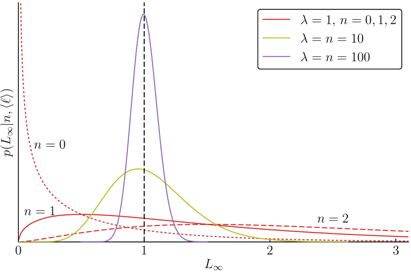
Consider the special case when the number of packets $K$ to determine ${\bm{\phi}}$ is large. Then we may consider ${\bm{\phi}}$ fixed, or equivalently $p({\bm{\phi}}\,|\,\mathcal{D})$ is a Dirac $\delta$ function, and we set $\mu$ to the sample mean from $K$ packets, $\mu({\bm{\phi}})=\mathchoice{\overline{\displaystyle\ell}}{\overline{\textstyle\ell}}{\overline{\scriptstyle\ell}}{\overline{\scriptscriptstyle\ell}}$. The Monte Carlo data are summarised by $N$ and $\mathchoice{\overline{\displaystyle\ell}}{\overline{\textstyle\ell}}{\overline{\scriptstyle\ell}}{\overline{\scriptscriptstyle\ell}}$ and there is no integral to perform:

$$p(L_{\infty}\,|\,N,\mathchoice{\overline{\displaystyle\ell}}{\overline{\textstyle\ell}}{\overline{\scriptstyle\ell}}{\overline{\scriptscriptstyle\ell}}) =\operatorname{Gamma}\quantity(\frac{L_{\infty}}{\mathchoice{\overline{\displaystyle\ell}}{\overline{\textstyle\ell}}{\overline{\scriptstyle\ell}}{\overline{\scriptscriptstyle\ell}}}\middle|N+\tfrac{1}{2},1)\frac{1}{\mathchoice{\overline{\displaystyle\ell}}{\overline{\textstyle\ell}}{\overline{\scriptstyle\ell}}{\overline{\scriptscriptstyle\ell}}}$$ (11)

The complete solution is just a rescaled $\operatorname{Gamma}$ distribution that is valid for any $N\geq 0$, $L_{\infty}>0$, and $\mathchoice{\overline{\displaystyle\ell}}{\overline{\textstyle\ell}}{\overline{\scriptstyle\ell}}{\overline{\scriptscriptstyle\ell}}>0$; see Figure 2. For ease of comparison with the literature (Section 2), the posterior mean and variance are

$$\operatorname{\mathbb{E}}\left[L_{\infty}\,|\,N,\mathchoice{\overline{\displaystyle\ell}}{\overline{\textstyle\ell}}{\overline{\scriptstyle\ell}}{\overline{\scriptscriptstyle\ell}}\right] =(N+\tfrac{1}{2})\mathchoice{\overline{\displaystyle\ell}}{\overline{\textstyle\ell}}{\overline{\scriptstyle\ell}}{\overline{\scriptscriptstyle\ell}},$$ (12)

$$\operatorname{\mathbb{V}}\left[L_{\infty}\,|\,N,\mathchoice{\overline{\displaystyle\ell}}{\overline{\textstyle\ell}}{\overline{\scriptstyle\ell}}{\overline{\scriptscriptstyle\ell}}\right] =(N+\tfrac{1}{2})\mathchoice{\overline{\displaystyle\ell}}{\overline{\textstyle\ell}}{\overline{\scriptstyle\ell}}{\overline{\scriptscriptstyle\ell}}^{2}.$$ (13)

as derived in Section 7.3. On the one hand, the variance increases with $N$ for fixed $\mathchoice{\overline{\displaystyle\ell}}{\overline{\textstyle\ell}}{\overline{\scriptstyle\ell}}{\overline{\scriptscriptstyle\ell}}$. On the other hand, if ${N_{p}}$ is increased such that $N\propto{N_{p}}$ and $\mathchoice{\overline{\displaystyle\ell}}{\overline{\textstyle\ell}}{\overline{\scriptstyle\ell}}{\overline{\scriptscriptstyle\ell}}\propto 1/{N_{p}}$ the variance on $L_{\infty}$ shrinks at the usual rate $1/{{N_{p}}}$ and the solution contracts around the true value with probability one as illustrated in Figure 2.

Figure 2: Contraction of the posterior for $L_{\infty}$ when increasing the total number of packets, ${N_{p}}$, in the simulation around the true value $L_{\infty}=1$. We set $\mathchoice{\overline{\displaystyle\ell}}{\overline{\textstyle\ell}}{\overline{\scriptstyle\ell}}{\overline{\scriptscriptstyle\ell}}=1/\lambda$ in Equation 11 where $\lambda\propto{N_{p}}$.

4 Gaussian model

For finite $K$, we have to specify the functional form $p(L\,|\,{\bm{\phi}})$. Focusing on a Gaussian model that simplifies calculations helps to illuminate the scaling behaviour. We conjecture that this model performs well in most applications due to asymptotic normality since all we really need from $p(L\,|\,{\bm{\phi}})$ to learn $L_{\infty}$ is $\mu({\bm{\phi}})=\operatorname{\mathbb{E}}\left[L\,|\,{\bm{\phi}}\right]$. In contrast, modelling $L$ is more sensitive to the higher moments of $p(L\,|\,{\bm{\phi}})$.

In the Bayesian interpretation, probability is the degree of belief in the truth of a statement conditional on all information included. In our case, the most interesting property of $p(L\,|\,{\bm{\phi}})$ is its mean $\mu$. Of minor importance is its variance $\sigma^{2}$ because it dictates how accurately we know $\mu$ from the finite number of packets. The maximum-entropy distribution for $L$ knowing the mean and variance is a Gaussian distribution, and its parameters are just $\mu$ and $\sigma^{2}$ if the contribution from the $\ell<0$ tail of the Gaussian is negligible, which we may safely assume if $K\gg 1$. We hence set ${\bm{\phi}}=(\mu,\sigma^{2})$ and

$$p(\ell\,|\,{\bm{\phi}})=p(\ell\,|\,\mu,\sigma^{2}) =\operatorname{\mathcal{N}}(\ell\,|\,\mu,\sigma^{2}).$$ (14)

Using Bayes’ theorem the posterior is

$$p(\mu,\sigma^{2}\,|\,\mathcal{D})=\operatorname{\mathcal{N}}(\mu\,|\,\mathchoice{\overline{\displaystyle\ell}}{\overline{\textstyle\ell}}{\overline{\scriptstyle\ell}}{\overline{\scriptscriptstyle\ell}},\tfrac{1}{K}\sigma^{2})\operatorname{InvGamma}\quantity(\sigma^{2}\middle|\tfrac{K}{2},\tfrac{K}{2}\mathchoice{\overline{\displaystyle\sigma^{2}}}{\overline{\textstyle\sigma^{2}}}{\overline{\scriptstyle\sigma^{2}}}{\overline{\scriptscriptstyle\sigma^{2}}})$$ (15)

for $\mu>0$ where we choose a conjugate Normal-$\operatorname{InvGamma}$ model with an uninformative prior; see Section 7.2 for details. Now the posterior depends on $\mathcal{D}$ only through $N$, $K$, and the statistics $\mathchoice{\overline{\displaystyle\ell}}{\overline{\textstyle\ell}}{\overline{\scriptstyle\ell}}{\overline{\scriptscriptstyle\ell}}$ and $\mathchoice{\overline{\displaystyle\sigma^{2}}}{\overline{\textstyle\sigma^{2}}}{\overline{\scriptstyle\sigma^{2}}}{\overline{\scriptscriptstyle\sigma^{2}}}$ computed from $K$ packets. Inserting Equation 15 into Equation 10, we have to approximate the integral using quadrature methods. We can, however, calculate mean and variance for $L_{\infty}$ analytically:

$$\operatorname{\mathbb{E}}\left[L_{\infty}\,|\,N,K,\mathchoice{\overline{\displaystyle\ell}}{\overline{\textstyle\ell}}{\overline{\scriptstyle\ell}}{\overline{\scriptscriptstyle\ell}},\mathchoice{\overline{\displaystyle\sigma^{2}}}{\overline{\textstyle\sigma^{2}}}{\overline{\scriptstyle\sigma^{2}}}{\overline{\scriptscriptstyle\sigma^{2}}}\right] =(N+\tfrac{1}{2})\mathchoice{\overline{\displaystyle\ell}}{\overline{\textstyle\ell}}{\overline{\scriptstyle\ell}}{\overline{\scriptscriptstyle\ell}},$$ (16)

$$\operatorname{\mathbb{V}}\left[L_{\infty}\,|\,N,K,\mathchoice{\overline{\displaystyle\ell}}{\overline{\textstyle\ell}}{\overline{\scriptstyle\ell}}{\overline{\scriptscriptstyle\ell}},\mathchoice{\overline{\displaystyle\sigma^{2}}}{\overline{\textstyle\sigma^{2}}}{\overline{\scriptstyle\sigma^{2}}}{\overline{\scriptscriptstyle\sigma^{2}}}\right] =(N+\tfrac{1}{2})\quantity(\frac{N+\tfrac{3}{2}}{K-2}\mathchoice{\overline{\displaystyle\sigma^{2}}}{\overline{\textstyle\sigma^{2}}}{\overline{\scriptstyle\sigma^{2}}}{\overline{\scriptscriptstyle\sigma^{2}}}+\mathchoice{\overline{\displaystyle\ell}}{\overline{\textstyle\ell}}{\overline{\scriptstyle\ell}}{\overline{\scriptscriptstyle\ell}}^{2});$$ (17)

see Section 7.3 for the derivation and further discussion.

5 Discussion

5.1 Comparison to experimental data

Figure 3: The convolution of simulation $p(L_{\infty}\,|\,\mathcal{D})$ and experimental uncertainty $p(L_{\rm obs}\,|\,L_{\infty},\sigma_{\rm obs}^{2})$ yields the likelihood $p(L_{\rm obs}\,|\,{\bm{\theta}})$.

The ultimate goal of the presented analysis is a likelihood to compare radiative-transfer models and experimental spectra. In a single bin, the likelihood $\mathcal{L}({\bm{\theta}}|L_{\rm obs})=p(L_{\rm obs}|{\bm{\theta}})$ with ${\bm{\theta}}$ denoting physics model parameters (e.g. abundances, temperatures, densities) and $L_{\rm obs}$ denoting the observed luminosity. This likelihood is the convolution of the probability distribution from the radiative-transfer code (as presented in this work) and the probability distribution for the observed luminosity (e.g. a Gaussian distribution)

$$p(L_{\rm obs}\,|\,{\bm{\theta}}) =\int\differential{L_{\infty}}p(L_{\infty}\,|\,\mathcal{D})p(L_{\rm obs}\,|\,L_{\infty},{\bm{\theta}})$$ (18)

$$=\int\differential{L_{\infty}}p(L_{\infty}\,|\,\mathcal{D})\operatorname{\mathcal{N}}(L_{\rm obs}\,|\,L_{\infty},\sigma_{\rm obs}^{2}).$$ (19)

Note that ${\bm{\theta}}$ only implicitly affects the simulation and experimental output in our graphical model (see Figure 1) and thus does not appear explicitly in the integrand.

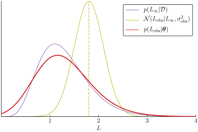
For simulation bins with a large number of packets (e.g. $N>25$), $p(L_{\infty}\,|\,\mathcal{D})$ may be accurately modelled by the Gaussian model of Section 4. The $\operatorname{Gamma}$ distribution in our general solution Equation 10 quickly converges to a Gaussian distribution for large $N$ such that the convolution reduces to the well known result of a Gaussian with variances added in quadrature:

$$p(L_{\rm obs}\,|\,{\bm{\theta}}) =\operatorname{\mathcal{N}}\quantity(L_{\rm obs}\middle|(N+\tfrac{1}{2})\,\mathchoice{\overline{\displaystyle\ell}}{\overline{\textstyle\ell}}{\overline{\scriptstyle\ell}}{\overline{\scriptscriptstyle\ell}},\sigma^{2}),$$ (20)

where

$$\sigma^{2} =\operatorname{\mathbb{V}}\left[L_{\infty}\middle|N,N,\mathchoice{\overline{\displaystyle\ell}}{\overline{\textstyle\ell}}{\overline{\scriptstyle\ell}}{\overline{\scriptscriptstyle\ell}},\mathchoice{\overline{\displaystyle\sigma^{2}}}{\overline{\textstyle\sigma^{2}}}{\overline{\scriptstyle\sigma^{2}}}{\overline{\scriptscriptstyle\sigma^{2}}}\right]+\sigma_{\rm obs}^{2},$$ (21)

where $\sigma_{\rm obs}^{2}$ is the variance of the observation model and the variance due to simulation uncertainty is given explicitly in Equation 17.

For bins with small $N$ we recommend numerical integration of Equation 18 using efficient cubature techniques (Genz & Malik, 1980; Johnson, 2017). Figure 3 illustrates the effect of the convolution: the resulting distribution $p(L_{\rm obs}\,|\,{\bm{\theta}})$ is smeared out taking into account both simulation and experimental uncertainty. In Figure 3, we choose the $\operatorname{Gamma}$ distribution of Equation 11, which requires $K\gg 1$, for $N=6$ and $\mathchoice{\overline{\displaystyle\ell}}{\overline{\textstyle\ell}}{\overline{\scriptstyle\ell}}{\overline{\scriptscriptstyle\ell}}=0.2$. In this case, the variance due to simulation from Equation 13 is 0.26 and dominates the experimental uncertainty $\sigma_{\rm obs}^{2}=0.3^{2}=0.09$.

In a Bayesian analysis, one would evaluate the presented likelihood for each frequency bin in every iteration of, for example, a Markov chain over ${\bm{\theta}}$ given the observed value $L_{\rm obs}$ as indicated by the dashed vertical line in Figure 3. For $L_{\rm obs}$ or $L_{\infty}$ close to zero, it is necessary to manually normalise the outcome to ensure that $\int_{L_{\rm obs}>0}\differential{L_{\rm obs}}p(L_{\rm obs}\,|\,{\bm{\theta}})=1$ because the convolution with the Gaussian $\operatorname{\mathcal{N}}(L_{\rm obs}\,|\,L_{\infty},\sigma_{\rm obs}^{2})$ may shift some probability mass into the unphysical region $L_{\rm obs}<0$. This effect is relevant even for parameter inference because the normalisation depends on ${\bm{\theta}}$. For the analytic result Equation 20, the correction can be done with the cumulative of the Gaussian distribution. For the numerical integration, we evaluate $p(L_{\rm obs}\,|\,{\bm{\theta}})$ on a grid of $L_{\rm obs}$ values instead of just the observed value, and then use, for example, Simpson’s quadrature rule to normalise. In the example of Figure 3, the normalisation was off by just 0.5 % function but upon increasing $\sigma_{\rm obs}^{2}$ from $0.3^{2}\to 1$, the normalisation is off by 12 %.

A simple example illustrates the potential computational savings of our method. Let us assume a reasonable relative experimental uncertainty $\sigma_{\rm obs}/L_{\rm obs}=5\%$. To achieve the same level of precision on $L_{\infty}$ in a typical tardis run with $\mathchoice{\overline{\displaystyle\ell}}{\overline{\textstyle\ell}}{\overline{\scriptstyle\ell}}{\overline{\scriptscriptstyle\ell}}=1.41,\mathchoice{\overline{\displaystyle\sigma^{2}}}{\overline{\textstyle\sigma^{2}}}{\overline{\scriptstyle\sigma^{2}}}{\overline{\scriptscriptstyle\sigma^{2}}}=0.001$, we solve

$$\frac{\sqrt{\operatorname{\mathbb{V}}\left[L_{\infty}\middle|N,N,\mathchoice{\overline{\displaystyle\ell}}{\overline{\textstyle\ell}}{\overline{\scriptstyle\ell}}{\overline{\scriptscriptstyle\ell}},\mathchoice{\overline{\displaystyle\sigma^{2}}}{\overline{\textstyle\sigma^{2}}}{\overline{\scriptstyle\sigma^{2}}}{\overline{\scriptscriptstyle\sigma^{2}}}\right]}}{\operatorname{\mathbb{E}}\left[L_{\infty}\,|\,N,N,\mathchoice{\overline{\displaystyle\ell}}{\overline{\textstyle\ell}}{\overline{\scriptstyle\ell}}{\overline{\scriptscriptstyle\ell}},\mathchoice{\overline{\displaystyle\sigma^{2}}}{\overline{\textstyle\sigma^{2}}}{\overline{\scriptstyle\sigma^{2}}}{\overline{\scriptscriptstyle\sigma^{2}}}\right]}=0.05$$ (22)

to find about $N=400$ samples in a bin are needed. Let us consider the simulation uncertainty to be irrelevant at the 1 % level. Then we would need $N=10000$, or 25 times more packets in the simulation.

5.2 Aspects of the derivation

The posterior means in Equation 12 and Equation 16 agree exactly and the variance Equation 13 is obtained from Equation 17 in the limit $N\ll K$. This is a good consistency check because the derivation of Equation 13 assumed $K\to\infty$ from the start. In the case $1\ll N\ll K$, mean and variance agree with the normal approximation in Equation 7 used previously when $N+\tfrac{1}{2}\approx N$. The extra $+\tfrac{1}{2}$ is due to our usage of the Jeffreys prior for $\lambda$; it leads to a reduced bias and reduced variance compared to a uniform prior that would contribute an extra $+1$, see Section 7.3 for further details. In contrast to the normal approximation, our posterior $p(L_{\infty}\,|\,\mathcal{D})$ is applicable for any $N$, even $N=0$. In that case, $K>2$ is required for finite variance and the larger $K$ is, the better. It is evident from the extra term $\propto\mathchoice{\overline{\displaystyle\sigma^{2}}}{\overline{\textstyle\sigma^{2}}}{\overline{\scriptstyle\sigma^{2}}}{\overline{\scriptscriptstyle\sigma^{2}}}$ in Equation 17 that including the sampling uncertainty of $\ell$ increases the variance on $L_{\infty}$, so the asymptotic approximation Equation 13 and the very similar literature result 7 may severely underestimate the total uncertainty on $L_{\infty}$ if $\sqrt{\mathchoice{\overline{\displaystyle\sigma^{2}}}{\overline{\textstyle\sigma^{2}}}{\overline{\scriptstyle\sigma^{2}}}{\overline{\scriptscriptstyle\sigma^{2}}}}/\mathchoice{\overline{\displaystyle\ell}}{\overline{\textstyle\ell}}{\overline{\scriptstyle\ell}}{\overline{\scriptscriptstyle\ell}}$ is of $\order{1}$, which occurs, for example, if $p(\ell\,|\,{\bm{\phi}})$ peaks near $\ell=0$.

5.3 Comparison to the compound Poisson

We stress again that we formulate a posterior for $L_{\infty}$ and we do not model the CPD for $L$ as for example Bohm & Zech (2014) do. We could also model the posterior predictive distribution for $L$ given the simulation output, $p(L\,|\,\mathcal{D})$. Although there is no fundamental problem, there are many more integrals to solve — in particular for small $N$ — instead of the single one in Equation 10, and the choice of $p(L\,|\,{\bm{\phi}})$ is crucial to getting a tractable result at all. We present the derivation in Section 7.4 that shows the same problems also hold true in a frequentist analysis. The conclusion from the posterior predictive is that the dominant contribution to the variance in the Bayesian case is $\propto 2n$, or just twice as large as in our central results of Equations 13 and 17 because there is Poisson uncertainty from the one observation of $N$ and the same uncertainty again in the prediction of a future output of the compound Poisson process. Another difference is that $p(L_{\infty}\,|\,\mathcal{D})$ is unimodal but $p(L\,|\,\mathcal{D})$ is multimodal due to superposition as in Equation 3, although the impact can be made small by suitable data preprocessing.

Coincidentally, someone who mistakes $L$ for $L_{\infty}$ and sets $\operatorname{\mathbb{E}}\left[\ell\,|\,{\bm{\phi}}\right]=\mathchoice{\overline{\displaystyle\ell}}{\overline{\textstyle\ell}}{\overline{\scriptstyle\ell}}{\overline{\scriptscriptstyle\ell}}$ ignoring all uncertainties except due to the Poisson process asymptotically gets very similar mean and variance as with our more general method; compare Equation 7 to Equations 12 and 13. But our method also applies for small $N$ and includes all uncertainties. In special cases, all integrals can even be done analytically.

6 Conclusion

In conclusion, our new method to treat statistical uncertainties in the estimation of the luminosity in a frequency bin based on packets from a Monte Carlo radiative-transfer simulation is superior to previous approaches in several ways. First, we present a proper posterior distribution that is easy to evaluate for any value of the luminosity, not just an error estimate. Second, our posterior is valid for large and small $N$, even for $N=0$ packets. Thus no bin should ever be discarded as each contains valuable information. Knowledge of the uncertainties allows to stop the simulation once a certain threshold is reached.

Future directions of research include a fundamental generalisation from independent bins and the Poisson model to bins coupled in a multinomial model. One would then predict the luminosities in all bins simultaneously. In a single bin, the Poisson rate $\lambda$ would correspond to $c\,{N_{p}}$, where $c$ is the probability for a packet to end up in this bin. The sum of those probabilities is one, a constraint that we do not use in our current formulation. Additional useful constraints include modelling $\mu$ as frequency-dependent, for example in a smooth fashion with a Gaussian process as in Rasmussen & Williams (2006) that, once trained, yields a Gaussian distribution for $\mu$ at every bin centre. Then the multi-dimensional integral over ${\bm{\phi}}$ in Equation 10 reduces to the simpler one-dimensional integral Equation 32 and the mean would be known very precisely in regions with many packets. The disadvantages include the extra computing effort to train the Gaussian process in every iteration of a fit, sensitivity to the hyperparameters of the Gaussian process, and an extra level of complexity where user attention is needed. One reason why $\mu$ could vary with the frequency is that the probability of scattering say a single photon on an iron atom depends on the frequency of the photon so the change of luminosity of a photon packets also depends on the frequency. Including extra constraints should lead to a tighter posterior on $\mu$ but it is not clear if tractable results can be obtained, and presumably they are not as easy to compute as in our current approach.

7 Appendix

7.1 Derivation of posterior for $L_{\infty}$

The first step is the posterior for $\lambda$ given $N$, the number of packets with a frequency in the bin under consideration. Bayes’ Theorem yields

$$p(\lambda\,|\,N) =\frac{p(N\,|\,\lambda)\,p(\lambda)}{p(N)}\ =\ \frac{p(N\,|\,\lambda)\,p(\lambda)}{\int\differential{\lambda}p(N\,|\,\lambda)\,p(\lambda)}$$ (23)

with the Poisson distribution

$$p(N\,|\,\lambda) =\frac{e^{-\lambda}\lambda^{N}}{N!}\quad N=0,1,\ldots,\infty.$$ (24)

The conjugate prior for $\lambda$ is the $\operatorname{Gamma}$ distribution with shape parameter $\alpha>0$ and rate parameter $\beta>0$ defined as

$$\operatorname{Gamma}(x\,|\,\alpha,\beta) =\frac{\beta^{\alpha}}{\Gamma(\alpha)}x^{\alpha-1}e^{-\beta x}\,,\quad 0\leq x<\infty.$$ (25)

With initial hyperparameters $\alpha_{0}$ and $\beta_{0}$, the posterior is

$$p(\lambda\,|\,N) =\operatorname{Gamma}(\lambda\,|\,\alpha=N+\alpha_{0},\,\beta=1+\beta_{0}).$$ (26)

We set $\beta_{0}=0$, which implies effectively no observations in the prior. For $\alpha_{0}$, we consider three options: $\alpha_{0}=1$ is a uniform prior, $\alpha_{0}=\tfrac{1}{2}$ is the prior advocated by Jeffreys (1946), which coincides with the reference prior by Bernardo (1979), and $\alpha_{0}=0$ is the transformation-group prior described by Jaynes (2003). The Jaynes prior is derived assuming $\lambda\propto$ measurement time and that any rescaling of time cannot change the state of knowledge. This prior is degenerate for an observation $N=0$ and thus not useful for us because it is common to have empty bins. We prefer the Jeffreys prior over the uniform prior because the former corresponds to a state of knowledge with minimum expected impact on the posterior and carries the same information in any one-to-one transformation of parameters, thus we set $\alpha_{0}=\tfrac{1}{2}$.

The second step is to choose a specific distribution for the luminosity of a single packet that comes out of the simulation, $p(L\,|\,{\bm{\phi}})$. This is problem dependent and we leave this decision unspecified. In any case, the posterior for ${\bm{\phi}}$ has the generic structure

$$p({\bm{\phi}}\,|\,\mathcal{D})\propto p({\bm{\phi}})\prod_{n=1}^{N}p(\ell_{n}\,|\,{\bm{\phi}}).$$ (27)

We assume that the luminosity distribution permits to calculate the mean luminosity $\mu({\bm{\phi}})$ analytically. Using the basic laws of probability, we can propagate the uncertainty on $\lambda$ and ${\bm{\phi}}$ to arrive at the desired posterior for $L_{\infty}=\lambda\mu({\bm{\phi}})$ using the Dirac $\delta$ function $p(L_{\infty}\,|\,\lambda,{\bm{\phi}})=\delta(L_{\infty}-\lambda\mu({\bm{\phi}}))$:

$$p(L_{\infty}\,|\,\mathcal{D}) =\int\differential{\lambda}\differential{{\bm{\phi}}}p(L_{\infty}\,|\,\lambda,{\bm{\phi}},\mathcal{D})p(\lambda,{\bm{\phi}}\,|\,\mathcal{D})$$ (28)

$$=\int\differential{\lambda}\differential{{\bm{\phi}}}p(L_{\infty}\,|\,\lambda,{\bm{\phi}})p(\lambda\,|\,N)p({\bm{\phi}}\,|\,\mathcal{D})$$ (29)

$$=\int\differential{\lambda}\differential{{\bm{\phi}}}\delta(L_{\infty}-\lambda\mu({\bm{\phi}}))$$

$$\quad\times\operatorname{Gamma}(\lambda\,|\,N+\tfrac{1}{2},1)p({\bm{\phi}}\,|\,\mathcal{D}).$$ (30)

Performing the integral over $\lambda$ with the help of the $\delta$ function, we arrive the general result

$$p(L_{\infty}\,|\,\mathcal{D}) =\int\differential{{\bm{\phi}}}\operatorname{Gamma}\quantity(\frac{L_{\infty}}{\mu({\bm{\phi}})}\middle|N+\tfrac{1}{2},1)\frac{p({\bm{\phi}}\,|\,\mathcal{D})}{\mu({\bm{\phi}})}.$$ (31)

Formally we can rewrite the result as a one-dimensional integral because ${\bm{\phi}}$ appears only through $\mu$

$$p(L_{\infty}\,|\,\mathcal{D}) =\int\differential{\mu}\operatorname{Gamma}\quantity(\frac{L_{\infty}}{\mu}\middle|N+\tfrac{1}{2},1)\frac{p(\mu\,|\,\mathcal{D})}{\mu}$$ (32)

but $p(\mu\,|\,\mathcal{D})$ requires a usually intractable integral over ${\bm{\phi}}$.

7.2 Details on the Gaussian model

The luminosity distribution $p(L\,|\,{\bm{\phi}})$ (see Equation 14) can be inferred from Monte Carlo data $\mathcal{D}=(K,{\bm{\ell}})$ with $K$ samples, where $K=N$ means packets from just one bin are used. For weak dependence on the frequency, one may use several adjacent bins such that $K>N$. Under the assumption that $p(L\,|\,{\bm{\phi}})$ is independent of the frequency, one can use all packets; i.e. $K={N_{p}}$. Assuming independent packets, the posterior is

$$p({\bm{\phi}}\,|\,\mathcal{D}) =p(\mu,\sigma^{2}\,|\,K,{\bm{\ell}})$$ (33)

$$=\frac{\prod_{k=1}^{K}\operatorname{\mathcal{N}}(\ell_{k}\,|\,\mu,\sigma^{2})\;p(\mu)\;p(\sigma^{2})}{p(\mathcal{D})}\,.$$ (34)

In keeping with prior information that luminosities are always positive, we assign a uniform prior $p(\mu\,|\,\mu_{\rm max})=1/\mu_{\rm max}$ independent of $N$; as before, the posterior is independent of $\mu_{\rm max}$ if chosen large enough. For $\sigma^{2}$, we use an Inverse Gamma prior with hyperparameters $(a_{0},b_{0})$,

$$p(\sigma^{2}\,|\,a_{0},b_{0}) =\operatorname{InvGamma}(\sigma^{2}\,|\,a_{0},b_{0})$$ (35)

$$=\frac{\quantity(b_{0})^{a_{0}}}{\Gamma(a_{0})}(\sigma^{2})^{-a_{0}-1}\exp(-b_{0}/\sigma^{2})$$ (36)

which is “conjugate” to the normal distribution likelihood of Equation 14 in that the posterior for $(\mu,\sigma^{2})$ is also a Gaussian in $\mu$ and an Inverse Gamma in $\sigma^{2}$,

$$p(\mu,\sigma^{2}\,|\,K,{\bm{\ell}},a_{0},b_{0}) =\operatorname{\mathcal{N}}(\mu\,|\,\mu_{K},\sigma_{K}^{2})$$

$$\quad\times\operatorname{InvGamma}(\sigma^{2}\,|\,a_{K},b_{K})$$ (37)

if the contribution from $\mu<0$ can be neglected. The hyperparameters are updated by the Monte Carlo data,

$$\mu_{K} =\mathchoice{\overline{\displaystyle\ell}}{\overline{\textstyle\ell}}{\overline{\scriptstyle\ell}}{\overline{\scriptscriptstyle\ell}},$$ (38)

$$\sigma_{K}^{2} =\frac{\sigma^{2}}{K},$$ (39)

$$a_{K} =a_{0}+\frac{K}{2},$$ (40)

$$b_{K} =b_{0}+\frac{K}{2}\mathchoice{\overline{\displaystyle\sigma^{2}}}{\overline{\textstyle\sigma^{2}}}{\overline{\scriptstyle\sigma^{2}}}{\overline{\scriptscriptstyle\sigma^{2}}}.$$ (41)

Results for small $K$ are inaccurate so one would typically pool more packets. In that case $K\gg 1$, the prior is less important and we may simply choose $a_{0}=b_{0}=0$ for a noninformative prior on $\sigma^{2}$.

7.3 Variance for $L_{\infty}$

Retaining the hyperparameter $\alpha_{0}$ of the prior $p(\lambda\,|\,\alpha_{0})$ (see Equation 26), the moments of the posterior $p(L_{\infty}\,|\,\mathcal{D})$ of Equation 31 for the asymptotic normal-inverse-gamma model where ${\bm{\phi}}=\mu,\sigma^{2}$ (see Equation 7.2) are

$$\operatorname{\mathbb{E}}\left[L_{\infty}^{r}\,|\,\mathcal{D}\right]= \int\differential{L_{\infty}}\differential{\mu}\differential{\sigma^{2}}\frac{L_{\infty}^{r}}{\mu}$$ (42)

$$\times\operatorname{Gamma}\quantity(\frac{L_{\infty}}{\mu}\,|\,N+\alpha_{0},1)$$

$$\times\mathcal{N}\quantity(\mu\,|\,\mu_{K},\sigma^{2}_{K})\operatorname{InvGamma}(\sigma^{2}\,|\,a_{K},b_{K})\,.$$

Using the definitions of $\mu_{K},a_{K},b_{K}$ in Equations 38–41 and the known first and second moments of the normal and inverse-gamma distributions, we find after some algebra

$$\operatorname{\mathbb{E}}\left[L_{\infty}\,|\,\mathcal{D}\right] =(N+\alpha_{0})\mathchoice{\overline{\displaystyle\ell}}{\overline{\textstyle\ell}}{\overline{\scriptstyle\ell}}{\overline{\scriptscriptstyle\ell}},$$ (43)

$$\operatorname{\mathbb{E}}\left[L_{\infty}^{2}\,|\,\mathcal{D}\right] =(N+\alpha_{0})(N+\alpha_{0}+1)\quantity(\mathchoice{\overline{\displaystyle\ell}}{\overline{\textstyle\ell}}{\overline{\scriptstyle\ell}}{\overline{\scriptscriptstyle\ell}}^{2}+\frac{\mathchoice{\overline{\displaystyle\sigma^{2}}}{\overline{\textstyle\sigma^{2}}}{\overline{\scriptstyle\sigma^{2}}}{\overline{\scriptscriptstyle\sigma^{2}}}}{K-2}),$$ (44)

where $\mathchoice{\overline{\displaystyle\ell}}{\overline{\textstyle\ell}}{\overline{\scriptstyle\ell}}{\overline{\scriptscriptstyle\ell}}$ and $\mathchoice{\overline{\displaystyle\sigma^{2}}}{\overline{\textstyle\sigma^{2}}}{\overline{\scriptstyle\sigma^{2}}}{\overline{\scriptscriptstyle\sigma^{2}}}$ are based on $K$ packets. From this the variance follows as

$$\operatorname{\mathbb{V}}\left[L_{\infty}\,|\,\mathcal{D}\right] =(N+\alpha_{0})\quantity(\frac{N+\alpha_{0}+1}{K-2}\mathchoice{\overline{\displaystyle\sigma^{2}}}{\overline{\textstyle\sigma^{2}}}{\overline{\scriptstyle\sigma^{2}}}{\overline{\scriptscriptstyle\sigma^{2}}}+\mathchoice{\overline{\displaystyle\ell}}{\overline{\textstyle\ell}}{\overline{\scriptstyle\ell}}{\overline{\scriptscriptstyle\ell}}^{2}).$$ (45)

Now let us focus on the special case with many packets in a bin; i.e. $N=K$ and $N\gg 1$:

$$\operatorname{\mathbb{V}}\left[L_{\infty}\,|\,\mathcal{D}\right]=N\mathchoice{\overline{\displaystyle\ell^{2}}}{\overline{\textstyle\ell^{2}}}{\overline{\scriptstyle\ell^{2}}}{\overline{\scriptscriptstyle\ell^{2}}}+\quantity[(2\alpha_{0}+1)\mathchoice{\overline{\displaystyle\ell^{2}}}{\overline{\textstyle\ell^{2}}}{\overline{\scriptstyle\ell^{2}}}{\overline{\scriptscriptstyle\ell^{2}}}-(\alpha_{0}+1)\mathchoice{\overline{\displaystyle\ell}}{\overline{\textstyle\ell}}{\overline{\scriptstyle\ell}}{\overline{\scriptscriptstyle\ell}}^{2}]+\order{\tfrac{1}{N}}.$$ (46)

where we set $N/(N-2)\to 1$. The three groups of terms allow an intuitive explanation. The dominant term $N\mathchoice{\overline{\displaystyle\ell^{2}}}{\overline{\textstyle\ell^{2}}}{\overline{\scriptstyle\ell^{2}}}{\overline{\scriptscriptstyle\ell^{2}}}$ captures the Poisson uncertainty inherent in the CPD. Ignoring the other terms, we see that if we average over the data distribution for fixed $\lambda$ and ${\bm{\phi}}$, we obtain the variance for the CPD given in Equation 8:

$$\operatorname{\mathbb{E}}\left[\operatorname{\mathbb{V}}\left[L_{\infty}\,|\,\mathcal{D}\right]\middle|\lambda,{\bm{\phi}}\right]$$

$$=\sum_{N}\int\differential{{\bm{\ell}}}p(N\,|\,\lambda)p\quantity({\bm{\ell}}\,|\,{\bm{\phi}})N\frac{1}{N}\sum_{n=1}^{N}\ell_{n}^{2}$$ (47)

$$=\sum_{N}p(N\,|\,\lambda)N\operatorname{\mathbb{E}}\left[\ell^{2}\,|\,{\bm{\phi}}\right]$$ (48)

$$=\lambda\operatorname{\mathbb{E}}\left[\ell^{2}\,|\,{\bm{\phi}}\right]=\lambda(\mu^{2}+\sigma^{2})=\operatorname{\mathbb{V}}\left[L\,|\,\lambda,{\bm{\phi}}\right].$$ (49)

In words, in the asymptotic regime our method that assumes $\lambda$ and ${\bm{\phi}}$ unknown on average yields a variance on the posterior for $L_{\infty}$ that is equal to the variance of the CPD for $L$ where $\lambda$ and ${\bm{\phi}}$ are assumed known! So with enough samples, the variance of the luminosities is irrelevant — there are $N$ samples to determine the moments — and only the Poisson uncertainty matters because it is inferred from a single observation.

The cross-terms in Equation 46 that are independent of $N$ are due to the simultaneous uncertainty of $\lambda$ and $\mu,\sigma^{2}$. Finally, the terms of $\order{1/N}$ follow the usual law for inferring mean and variance from $N$ identically distributed samples.

The cross-terms show the quantitative effect of the hyperparameter $\alpha_{0}$ in the prior for $\lambda,p(\lambda\,|\,\alpha_{0})$. The flat prior ($\alpha_{0}=1$) yields the largest variance, the Jaynes prior ($\alpha_{0}=0$) yields the smallest, and Jeffreys prior ($\alpha_{0}=1/2$) leads to something in between:

$$(2\alpha_{0}+1)\mathchoice{\overline{\displaystyle\ell^{2}}}{\overline{\textstyle\ell^{2}}}{\overline{\scriptstyle\ell^{2}}}{\overline{\scriptscriptstyle\ell^{2}}}-(\alpha_{0}+1)\mathchoice{\overline{\displaystyle\ell}}{\overline{\textstyle\ell}}{\overline{\scriptstyle\ell}}{\overline{\scriptscriptstyle\ell}}^{2}=\begin{cases}3\mathchoice{\overline{\displaystyle\sigma^{2}}}{\overline{\textstyle\sigma^{2}}}{\overline{\scriptstyle\sigma^{2}}}{\overline{\scriptscriptstyle\sigma^{2}}}+\mathchoice{\overline{\displaystyle\ell}}{\overline{\textstyle\ell}}{\overline{\scriptstyle\ell}}{\overline{\scriptscriptstyle\ell}}^{2},&\text{flat}\\ 2\mathchoice{\overline{\displaystyle\sigma^{2}}}{\overline{\textstyle\sigma^{2}}}{\overline{\scriptstyle\sigma^{2}}}{\overline{\scriptscriptstyle\sigma^{2}}}+1/2\mathchoice{\overline{\displaystyle\ell}}{\overline{\textstyle\ell}}{\overline{\scriptstyle\ell}}{\overline{\scriptscriptstyle\ell}}^{2},&\text{Jeffreys}\,.\\ \mathchoice{\overline{\displaystyle\sigma^{2}}}{\overline{\textstyle\sigma^{2}}}{\overline{\scriptstyle\sigma^{2}}}{\overline{\scriptscriptstyle\sigma^{2}}},&\text{Jaynes}\\ \end{cases}$$ (50)

Repeating the calculation for fixed ${\bm{\phi}}$, or $K\to\infty$, as in Equation 11, the $r$-th moment is

$$\operatorname{\mathbb{E}}\left[L_{\infty}^{r}\,|\,\mathcal{D}\right]=\int\differential{L_{\infty}}\frac{L_{\infty}^{r}}{\mu}\operatorname{Gamma}\quantity(\frac{L_{\infty}}{\mu}\,|\,N+\alpha_{0},1)$$

and we obtain the same mean as in Equation 43 and the variance

$$\operatorname{\mathbb{V}}\left[L_{\infty}\,|\,\mathcal{D}\right]=(N+\alpha_{0})\mathchoice{\overline{\displaystyle\ell}}{\overline{\textstyle\ell}}{\overline{\scriptstyle\ell}}{\overline{\scriptscriptstyle\ell}}^{2},$$ (52)

which is the limit of Equation 45 as $K\to\infty$. Interestingly, now the variance only depends on the first moment whereas in Equation 46 it is $\propto\mathchoice{\overline{\displaystyle\ell^{2}}}{\overline{\textstyle\ell^{2}}}{\overline{\scriptstyle\ell^{2}}}{\overline{\scriptscriptstyle\ell^{2}}}$ for large $N$. What seems like a paradox is a direct consequence of probability theory as an extension of logic. If we assume from the start that $\operatorname{\mathbb{E}}\left[L\right]$ is known, then all other properties of $p(L\,|\,{\bm{\phi}})$ are irrelevant with regard to inferring $L_{\infty}$. If on the contrary, we have to infer the mean from the Monte Carlo data, then it matters how large the variance of $p(L\,|\,{\bm{\phi}})$ is because the smaller the variance, the better the mean can be inferred from a fixed number of samples. Since in practice we do not know ${\bm{\phi}}$, we recommend Equation 45 to estimate $\operatorname{\mathbb{V}}\left[L_{\infty}\,|\,\mathcal{D}\right]$. This follows the recommendation by Jaynes (2003) to perform calculations for finite $N$ and to take the limit $N\to\infty$ only in the very end to avoid a paradox.

7.4 Variance for $L$

Repeating Equation 3, the basic definition of the CPD is

$$p(L\,|\,\lambda,{\bm{\phi}})=\sum_{N=0}^{\infty}p(N\,|\,\lambda)\;p(L\,|\,N,{\bm{\phi}}).$$ (53)

To obtain the posterior predictive given $\mathcal{D}$, we have to average over the posterior for $\lambda$ and ${\bm{\phi}}$ given in Equations 26 and 33:

$$p(L\,|\,\mathcal{D})=\int\differential{\lambda}\differential{{\bm{\phi}}}\;p(L\,|\,\lambda,{\bm{\phi}})\;p(\lambda\,|\,\mathcal{D})\;p({\bm{\phi}}\,|\,\mathcal{D}).$$ (54)

The second term on the right in Equation 53 can be expressed as a convolution upon expanding with the $N$ packet luminosities ${\bm{\ell}}$

$$p(L\,|\,N,{\bm{\phi}}) =\int\differential{{\bm{\ell}}}\;p(L\,|\,N,{\bm{\ell}})\;p({\bm{\ell}}\,|\,N,{\bm{\phi}})$$ (55)

$$=\int\differential{{\bm{\ell}}}\;\delta(L-\textstyle\sum_{n=1}^{N}\ell_{n})\;\prod_{n=1}^{N}p(\ell_{n}\,|\,{\bm{\phi}}).$$ (56)

To get a tractable expression, it is convenient to choose $p(\ell\,|\,{\bm{\phi}})$ such that the integral in Equation 55 can be solved analytically. This occurs for stable distributions for which the sum of luminosities follows the same distribution as each individual luminosity, although with different ${\bm{\phi}}$. Examples include the Gaussian model of Section 7.2 where $L\sim\operatorname{\mathcal{N}}\quantity(N\mu,N\sigma^{2})$ or a $\operatorname{Gamma}$ model where $p(\ell\,|\,{\bm{\phi}})=\operatorname{Gamma}(\ell\,|\,\alpha,\beta)$ and $L\sim\operatorname{Gamma}(N\alpha,\beta)$. The latter has the advantage that it automatically excludes $\ell<0$. In either case, for $\lambda$ large, the central limit theorem for the CPD holds, which eliminates both $\sum_{N}$ and $\int\differential{{\bm{\ell}}}$; see Bening & Korolev (2002, Theorem 4.3.1):

$$p(L\,|\,\lambda,{\bm{\phi}}) =\operatorname{\mathcal{N}}\quantity(L\,|\,\lambda\mu,\lambda(\mu^{2}{+}\sigma^{2})).$$ (57)

Repeating the calculation for the moments with this Gaussian approximation for the posterior predictive for $L$,

$$\operatorname{\mathbb{E}}\left[L^{r}\,|\,\mathcal{D}\right]= \int\differential{L}\differential{\lambda}\differential{\mu}\differential{\sigma^{2}}L^{r}\operatorname{\mathcal{N}}\quantity(L\,|\,\lambda\mu,\lambda(\mu^{2}{+}\sigma^{2}))$$

$$\times\operatorname{Gamma}\quantity(\lambda\,|\,N+\alpha_{0},1)$$ (58)

$$\times\mathcal{N}\quantity(\mu\,|\,\mu_{K},\sigma^{2}_{K})\operatorname{InvGamma}(\sigma^{2}\,|\,a_{K},b_{K})\,.$$

we find

$$\operatorname{\mathbb{E}}\left[L\,|\,\mathcal{D}\right] =(N+\alpha_{0})\mathchoice{\overline{\displaystyle\ell}}{\overline{\textstyle\ell}}{\overline{\scriptstyle\ell}}{\overline{\scriptscriptstyle\ell}},$$ (59)

$$\operatorname{\mathbb{E}}\left[L^{2}\,|\,\mathcal{D}\right] =(N+\alpha_{0})$$ (60)

$$\quad\times\bigg{\{}(N+\alpha_{0}+2)\quantity(\mathchoice{\overline{\displaystyle\ell}}{\overline{\textstyle\ell}}{\overline{\scriptstyle\ell}}{\overline{\scriptscriptstyle\ell}}^{2}+\frac{\mathchoice{\overline{\displaystyle\sigma^{2}}}{\overline{\textstyle\sigma^{2}}}{\overline{\scriptstyle\sigma^{2}}}{\overline{\scriptscriptstyle\sigma^{2}}}}{K-2})+\frac{\mathchoice{\overline{\displaystyle\sigma^{2}}}{\overline{\textstyle\sigma^{2}}}{\overline{\scriptstyle\sigma^{2}}}{\overline{\scriptscriptstyle\sigma^{2}}}}{1-2/K}\bigg{\}}.$$

Again setting $N=K$ and $N/(N-2)\to 1$ for large $N$ yields

$$\operatorname{\mathbb{V}}\left[L\,|\,\mathcal{D}\right]=2n\mathchoice{\overline{\displaystyle\ell^{2}}}{\overline{\textstyle\ell^{2}}}{\overline{\scriptstyle\ell^{2}}}{\overline{\scriptscriptstyle\ell^{2}}}+\quantity[(3\alpha_{0}-2)\mathchoice{\overline{\displaystyle\ell^{2}}}{\overline{\textstyle\ell^{2}}}{\overline{\scriptstyle\ell^{2}}}{\overline{\scriptscriptstyle\ell^{2}}}-(8-\alpha_{0})\mathchoice{\overline{\displaystyle\ell}}{\overline{\textstyle\ell}}{\overline{\scriptstyle\ell}}{\overline{\scriptscriptstyle\ell}}^{2}]+\order{\tfrac{1}{N}}.$$ (61)