A Fast Trajectory Optimization Framework for Legged Robots unifying ZMP and Capture Point Approaches

Fast Trajectory Optimization for Legged Robots
using Vertex-based ZMP Constraints

Abstract

This paper combines the fast Zero-Moment-Point (ZMP) approaches that work well in practice with the broader range of capabilities of a Trajectory Optimization formulation, by optimizing over body motion, footholds and Center of Pressure simultaneously. We introduce a vertex-based representation of the support-area constraint, which can treat arbitrarily oriented point-, line-, and area-contacts uniformly. This generalization allows us to create motions such quadrupedal walking, trotting, bounding, pacing, combinations and transitions between these, limping, bipedal walking and push-recovery all with the same approach. This formulation constitutes a minimal representation of the physical laws (unilateral contact forces) and kinematic restrictions (range of motion) in legged locomotion, which allows us to generate various motion in less than a second. We demonstrate the feasibility of the generated motions on a real quadruped robot.

I Introduction

Planning and executing motions for legged systems is a complex task. A central difficulty is that legs cannot pull on the ground, e.g. the forces acting on the feet can only push upwards. Since the motion of the body is mostly generated by these constrained (=unilateral) contact forces, this motion is also restricted. When leaning forward past the tip of your tows, you will fall, since your feet cannot pull down to generate a momentum that counteracts the gravity acting on your Center of Mass (CoM). Finding motions that respect these physical laws can be tackled by various approaches described in the following.

A successful approach to tackle this problem is through full-body Trajectory Optimization (TO), in which an optimal body and endeffector motion plus the appropriate inputs are discovered to achieve a high-level goal. This was demonstrated by [1, 2, 3, 4, 5, 6, 7] resulting in an impressive range of motions for legged systems. These TO approaches have shown great performance, but are often time consuming to calculate and not straight-forward to apply on a real robot. In [8] the authors generate an wide range of quadruped gaits, transitions and jumps based on a parameterized controller and periodic motions. While the resulting motions are similar to ours, the methods are very different: While our approach is based on TO with physical constraints, [8] optimizes controller parameters based mainly on motion capture data.

Previous research has shown that to generate feasible motions to execute on legged systems, non-TO approaches also work well, although the motions cannot cover the range of the approaches above. One way is to model the robot as a Linear Inverted Pendulum (LIP) and keep the Zero-Moment-Point (ZMP) [9] inside the convex hull of the feet in stance. This approach has been successfully applied to generate motions for biped and quadruped walking [10, 11, 12, 13]. However, these hierarchical approaches use predefined footholds, usually provided by a higher-level planner beforehand that takes terrain information (height, slope) into account. Although this decoupling of foothold planning and body motion generation reduces complexity, it is unnatural, as the main intention of the footholds is to assist the body to achieve a desired motion. By providing fixed foot-trajectories that the body motion planner cannot modify, constraints such as stability or kinematic reachability become purely the responsibility of the lower-level body motion planner, artificially constraining the solution. A somewhat reverse view of the above are Capture Point (CP)[14] approaches, which have been successfully used to generate dynamic trotting and push recovery motions for quadruped robots [15, 16]. A desired body motion (usually a reference CoM velocity) is given by a high-level planner or heuristic, and a foothold/Center of Pressure (CoP) trajectory must be found that generates it.

Because of the dependency between footholds and body motion, approaches that optimize over both these quantities simultaneously, while still using a simplified dynamics model, have been developed [17, 18, 19, 20, 21, 22]. This reduces heuristics while increasing the range of achievable motions, but still keeps computation time short compared to full body TO approaches. These approaches are most closely related to the work presented in this paper.

The approaches [18, 19, 20, 21] demonstrate impressive performance on biped robots. One common difficulty in these approaches however is the nonlinearity of the CoP constraint with respect to the orientation of the feet. In [19, 20] the orientation is either fixed or solved with a separate optimizer beforehand. In [21] the nonlinearity of this constraint is accepted and the resulting nonlinear optimization problem solved. However, although the orientation of the individual feet can be optimized over in these approaches, a combined support-area with multiple feet in contact is often avoided, by not sampling the constraint during the double-support phase. For biped robots neglecting the constraint in the double-support phase is not so critical, as these take up little time during normal walking. For quadruped robots however, there are almost always two or more feet in contact at a given time, so the correct representation of the dynamic constraint in this phase is essential.

We therefore extend the capabilities of the approaches above by using a vertex-based representation of the CoP constraint, instead of hyperplanes. In [23] this idea is briefly touched, however the connection between the corners of the foot geometry and the convexity variables is not made and thereby the restriction of not sampling in the double-support phase remains. Through our proposed formulation, double- and single-stance support areas can be represented for arbitrary foot geometry, including point-feet. Additionally, it allows to represent arbitrarily oriented 1D-support lines, which wasn’t possible with the above approaches. Although not essential for biped walk on flat feet, this is a core necessity for dynamic quadruped motions (trot, pace, bound). This is a reason why ZMP-based approaches were so far only used for quadrupedal walking, where 2D-support areas were present.

The approach presented in this paper combines the LIP-based ZMP approaches that are fast and work well in practice with the broader range of capabilities of a TO formulation. A summary of the explicit contributions with respect to the papers above are:

• We reformulate the traditional ZMP-based legged locomotion problem [10] into a standard TO formulation with the CoP as input, clearly identifying state, dynamic model and path- and boundary-constraints, which permits easier comparison with existing methods in the TO domain. Push recovery behavior also naturally emerges from this formulation.

• We introduce a vertex-based representation of the CoP constraint, instead of hyperplanes. which allows us to treat arbitrarily oriented point-, line-, and area-contacts uniformly. This enables us to generate motions that are difficult for other ZMP-based approaches, such as bipedal walk with double-support phases, point-feet locomotion, various gaits as well as arbitrary combinations and transitions between these.

• Instead of the heuristic shrinking of support areas, we introduce a cost term for uncertainties that improve the robustness of the planned motions.

We demonstrate that the problem can be solved for multiple steps in less than a second to generate walking, trotting, bounding, pacing, combinations and transitions between these, limping, biped walking and push-recovery motions for a quadruped robot. Additionally, we verify the physically feasibility of the optimized motions through demonstration of walking and trotting on a real $80\text{\,}\mathrm{kg}$ hydraulic quadruped.

II Method

II-A Physical Model

We model the legged robot as a Linear Inverted Pendulum (LIP), with its CoM ${\mathbf{c}\!=\!(c_{x},c_{y})}$ located at a constant height $h$. The touchdown position of the pendulum with the ground (also known as ZMP or CoP) is given by ${\mathbf{u}\!=\!(u_{x},u_{y})}$ as seen in Fig. 1. The CoM acceleration $\ddot{\mathbf{c}}$ is predefined by the physics of a tipping pendulum

$$\begin{bmatrix}\dot{\mathbf{c}}\\ \ddot{\mathbf{c}}\end{bmatrix} =\mathbf{f}(\mathbf{x},\mathbf{u})=\begin{bmatrix}\dot{\mathbf{c}}\\ (\mathbf{c}-\mathbf{u})gh^{-1}\end{bmatrix}.$$ (1)

The second-order dynamics are influenced by the CoM position $\mathbf{c}$, the CoP $\mathbf{u}$ and gravity $g$. This model can be used to describe a legged robot, since the robot can control the torques in the joints, thereby the contact forces and through these the position of the CoP. Looking only at the x-direction (left image in Fig. 1), if the robot decides to lift the hind leg, the model describing the system dynamics is a pendulum in contact with the ground at the front foot $\mathbf{p}^{RF}$, so ${\mathbf{u}\!=\!\mathbf{p}^{RF}\!=\!(p_{x},p_{y})}$. Since this pendulum is nearly upright, the CoM will barely accelerate in x; the robot is balancing on the front leg. However, lifting the front leg can be modeled as placing the pendulum at ${\mathbf{u}=\mathbf{p}^{LH}}$, which is strongly leaning and thereby must accelerate forward in x. By distributing the load between the legs, the robot can generate motions corresponding to a pendulum anchored anywhere between the contact points, e.g. $\mathbf{u}\in\mathcal{P}$ (see Fig. 1). Therefore, the CoP $\mathbf{u}$ is considered the input to the system and an abstraction of the joint torques and contact forces.

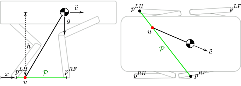
Figure 1: Modeling of a quadruped robot by a LIP with the right-front $\mathbf{p}^{RF}$ and left-hind $\mathbf{p}^{LH}$ legs in contact. Through joint torques the robot can control the center of pressure $\mathbf{u}$ and thereby the motion of the CoM $\ddot{\mathbf{c}}$. However, $\mathbf{u}$ can only lie inside the convex hull (green line) of the contact points.

II-B Trajectory Optimization Problem

We want to obtain the inputs $\mathbf{u}(t)$ that generate a motion $\mathbf{x}(t)$ from an initial state $\mathbf{x}_{0}$ to a desired goal state $\mathbf{x}_{T}$ in time $T$ for a robot described by the system dynamics $\mathbf{f}(\mathbf{x},\mathbf{u})$, while respecting some constraints $\mathbf{h}(\mathbf{x},\mathbf{u})\leq 0$ and optimizing a performance criteria $J$. This can be formulated as a continuous-time TO problem

$$\text{find \hskip 36.98866pt}\mathbf{x}(t),\mathbf{u}(t) ,\quad\text{for }t\in[0,T]$$ (2a)

$$\text{subject to}\hskip 14.22636pt\mathbf{x}(0)-\mathbf{x}_{0} =0\quad\text{ (given initial state)}$$ (2b)

$$\dot{\mathbf{x}}(t)-\mathbf{f}(\mathbf{x}(t),\mathbf{u}(t)) =0\quad\text{ (dynamic model)}$$ (2c)

$$\mathbf{h}(\mathbf{x}(t),\mathbf{u}(t)) \leq 0\quad\text{ (path constraints)}$$ (2d)

$$\mathbf{x}(T)-\mathbf{x}_{T} =0\quad\text{ (desired final state)}$$ (2e)

$$\mathbf{x}(t),\mathbf{u}(t) =\operatorname*{arg\,min}J(\mathbf{x},\mathbf{u}).$$ (2f)

The dynamics are modeled as those of a LIP (1), whereas the state and input for the legged system model are given by

$$\mathbf{x}(t) =\begin{bmatrix}\mathbf{c}&\dot{\mathbf{c}}&\mathbf{p}^{1},\alpha^{1},\dots,\mathbf{p}^{n_{f}},\alpha^{n_{f}}\end{bmatrix}^{T}$$ (3)

$$\mathbf{u}(t) =\mathbf{u},$$ (4)

which includes the CoM position and velocity and the position and orientation of the ${n_{f}}$ feet. The input $\mathbf{u}(t)$ to move the system is the generated CoP, abstracting the usually used contact forces or joint torques.

II-C Specific Case: Capture Point

We briefly show that this general TO formulation, using the LIP model, also encompasses Capture Point methods to generate walking motions. Consider the problem of finding the position to step with a point-foot robot to recover from a push. With the initial position $\mathbf{c}_{0}$ and the initial velocity $\dot{\mathbf{c}}_{0}$ generated by the force of the push we have ${\mathbf{x}_{0}\!=\!(\mathbf{c}_{0},\dot{\mathbf{c}}_{0})}$. The robot should come to, and remain, at a stop at the end of the motion, irrespective of where and when, so we have ${\dot{\mathbf{c}}_{T\to\infty}\!=\!0}$. We parametrize the input by the constant parameter ${\mathbf{u}(t)\!=\!\mathbf{u}_{0}}$, as we only allow one step with a point-foot. We allow the CoP to be placed anywhere, e.g. no path constraints (2d) and do not have a preference as to how the robot achieves this task, e.g. ${J(\mathbf{x},\mathbf{u})\!=\!0}$.

Such a simple TO problem can be solved analytically, without resorting to a mathematical optimization solver (see Appendix -A). The point on the ground to generate and hold the CoP in order to achieve a final steady-state maintaining zero CoM velocity becomes

$$\mathbf{u}(t)=\mathbf{u}_{0}=\mathbf{c}_{0}+\dot{\mathbf{c}}_{0}hg^{-1}.$$ (5)

This is the one-step Capture Point (CP), originally derived by [14] and the solution of our general TO formulation (2) for a very specific case (e.g one step/control input, zero final velocity).

II-D General Case: Legged Locomotion Formulation

Compared to the above example, our proposed formulation adds the capabilities to represent motions of multiple steps, time-varying CoP, physical restrictions as to where the CoP can be generated and preferences which of the feasible motions to choose. This TO formulation is explained on a high-level in the following, corresponding to Fig. 2, whereas more specific details of the implementation are postponed to the next section.

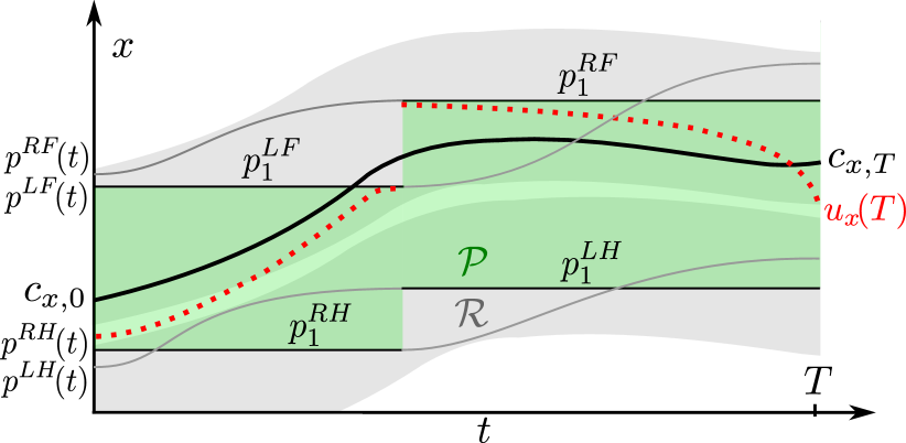
Figure 2: Overview of the TO problem: A point-foot quadruped robot trotting forward in x-direction, first swinging right-front and left-hind legs ${f\in\{RF,LH\}}$, then left-front and right-hind ${f\in\{LF,RH\}}$. The CoM motion $c_{x}$ (black line) is generated by shifting the CoP $u_{x}(t)$ (red dots). However, $u_{x}$ can only lie in the convex hull $\mathcal{P}$ (green area) of the legs in contact at that time $t$. Additionally, the position of each leg $p^{f}$ must always be inside its range of motion $\mathcal{R}$ (gray areas for front and hind legs) relative to the CoM. The optimization problem consist of varying the position of the footholds $p^{f}_{s}\in\mathcal{R}$, to allow inputs $u_{x}\in\mathcal{P}$ that drive the robot from an initial position $c_{x,0}$ to a desired goal position $c_{x,T}$ in time $T$.

II-D1 Unilateral Forces

We clearly differentiate between the CoP $\mathbf{u}$ and the feet positions $\mathbf{p}^{f}$, which only coincide for a point-foot robot with one leg in contact. Generally, the footholds affect the input bounds of $\mathbf{u}$. We use $\mathbf{u}$ to control the body, but must at the same time choose appropriate footholds to respect the unilateral forces constraint. Traditional ZMP approaches fix the footholds $\mathbf{p}^{f}$ in advance, as the combination of both the CoP $\mathbf{u}$ and the footholds make this constraint nonlinear. We accept this nonlinearity and the higher numerical complexity associated with it. This gives us a much larger range of inputs $\mathbf{u}$, as we can “customize” our bounds $\mathcal{P}$ by modifying the footholds according to the desired task. Therefore, the first path constraint of our TO problem is given by

$$\mathbf{h}_{1}(\mathbf{x}(t),\mathbf{u}(t))\leq 0\quad\Leftrightarrow\quad\mathbf{u}\in\mathcal{P}(\mathbf{p}^{f},\alpha^{f},c^{f}),$$ (6)

where $\mathcal{P}$ represents the convex hull of the feet in contact as seen in Fig. 2 and $c^{f}\in\{0,1\}\in\mathbb{Z}$ is the indicator if foot $f$ is in contact.

We implement this convex hull constraint by weighing the vertices/corners of each foot in contact. This extends the capabilities of traditional representations by line segments/hyperplanes to also model point- and line-contacts of arbitrary orientation. We use predefined contact sequences and timings $c^{f}(t)$, to only optimize over real-valued decision variables $w\in$ and not turn the problem into a mixed-integer Nonlinear Programming Problem (NLP). Simply by adapting this contact schedule $c^{f}(t)$, the optimizer generates various gaits as well as combinations and transitions between these, for which previously separate frameworks were necessary.

II-D2 Kinematic Reachability

When modifying the footholds to enclose the CoP, we must additionally ensure that these stay inside the kinematic range $\mathcal{R}$ of the legs (Reachability). This constraint that depends on both the CoM $\mathbf{c}$ and foothold positions $\mathbf{p}^{f}$ is formulated for every leg $f$ as

$$\mathbf{h}_{2}(\mathbf{x}(t))\leq 0\quad\Leftrightarrow\quad\mathbf{p}^{f}\in\mathcal{R}(\mathbf{c}).$$ (7)

Allowing the modification of both these quantities simultaneously characterizes the legged locomotion problem more accurately and reduces heuristics used in hierarchical approaches.

II-D3 Robust Motions

With the above constraints the motion will comply to physics and the kinematics of the system. This feasible motion is assuming a simplified model, a perfect tracking controller and an accurate initial state. To make solutions robust to real world discrepancies where these assumptions are violated, it is best to avoid the borders of feasible solutions, where the inequality constraints are tight (${\mathbf{h}\!=\!\mathbf{0}}$). This can be achieved by artificially shrinking the solutions space by a stability margin (e.g. ${\mathbf{h}\!\leq\!\mathbf{m}}$). For legged locomotion this is often done by shrinking the support area to avoid solutions were the CoP is placed at the marginally-stable border [11].

We do not restrict the solution space, but choose the more conservative of the feasible motions through a performance criteria $J_{\lambda}$. This soft constraint expresses “avoid boundaries when possible, but permit if necessary”. The robot is allowed to be at marginally stable states, but since there are many uncertainties in our model and assumptions, it is safer to avoid them. This cost does not require a hand-tuned stability margin and the solution can still be at the boundaries when necessary. However, especially for slow motions (e.g. walking) where small inaccuracies can accumulate and cause the robot to fall, this cost term is essential to generate robust motions for real systems.

III Implementation

There exist different methods to solve Optimal Control problems (2), namely Dynamic Programming (Bellman Optimality Equation), indirect (Maximum Principle) and direct methods [24]. In direct methods the continuous time TO problem is represented by a finite number of decision variables and constraints and solved by a nonlinear programming solver. If the decision variables $\mathbf{w}$ fully describe the input $\mathbf{u}(t)$ and state $\mathbf{x}(t)$ over time, the method is further classified as a simultaneous direct method, with flavors Direct Transcription and Multiple Shooting. In our approach we chose a Direct Transcription formulation, e.g. optimizing state and controls together. This has the advantage of not requiring an ODE solver, constraints on the state can be directly formulated and the sparse structure of the Jacobian often improves convergence. The resulting discrete formulation to solve the continuous problem in (2) is given by

find $$\mathbf{w}=(\mathbf{w}_{c},\mathbf{w}_{p},\mathbf{w}_{u})$$

subject to $$(\ref{eq:initial_constraints}),\hskip 76.82234pt\text{(given initial state)}$$

$$(\ref{eq:com_continuity}),(\ref{eq:com_accel_constraint}),(\ref{eq:kinematic_constraints}),(\ref{eq:convexity_all})\hskip 14.22636pt\text{(path-constraints)}$$

$$(\ref{eq:terminal_constraints}),\hskip 76.82234pt\text{(desired final state)}$$

$$\mathbf{w}=\operatorname*{arg\,min}(\ref{eq:lambda_cost}),\hskip 22.76228pt\text{(robustness cost)}$$

where $\mathbf{w}_{c}$ are the parameters describing the CoM motion, $\mathbf{w}_{p}$ the feet motion (swing and stance) and $\mathbf{w}_{u}$ the position of the CoP. This section describes in detail how we parametrize the state $(\mathbf{w}_{c},\mathbf{w}_{p})$ and input $\mathbf{w}_{u}$, formulate the path-constraints and defined the cost (21).

III-A Center-of-Mass Motion

This section explains how the continuous motion of the CoM can be described by a finite number of variables to optimize over, while ensuring compliance with the LIP dynamics.

III-A1 CoM Parametrization

The CoM motion is described by a spline, strung together by $n$ quartic-polynomials as

$$\mathbf{x}(t) =\begin{bmatrix}\mathbf{c}(t)\\ \dot{\mathbf{c}}(t)\end{bmatrix}=\sum_{i=1}^{4}\begin{bmatrix}(t\!-\!t_{k})\\ i\end{bmatrix}\mathbf{a}_{k,i}(t\!-\!t_{k})^{i\!-\!1}+\begin{bmatrix}\mathbf{a}_{k,0}\\ \mathbf{0}\end{bmatrix}$$ (8)

$$\mathbf{w}_{c} =\begin{bmatrix}\mathbf{a}_{1,0},\dots,\mathbf{a}_{1,4},\dots,\mathbf{a}_{n,0},\dots,\mathbf{a}_{n,4}\end{bmatrix},$$ (9)

with coefficients $\mathbf{a}_{k,i}\in 2$ and $t_{k}$ describing the global time at the start of polynomial $k$.

We ensure continuity of the spline by imposing equal position and velocity at each of the $n\!-\!1$ junctions between polynomial $k$ and $k\!+\!1$, so $\mathbf{x}[t_{k+1}^{-}]=\mathbf{x}[t_{k+1}^{+}]$. Using $T_{k}=t_{k+1}\!-\!t_{k}$ we enforce

$$\sum_{i=1}^{4}\begin{bmatrix}T_{k}\\ i\end{bmatrix}\mathbf{a}_{k,i}T_{k}^{i-1}+\begin{bmatrix}\mathbf{a}_{k,0}\\ \mathbf{0}\end{bmatrix}\!=\!\begin{bmatrix}\mathbf{a}_{k+1,0}\\ \mathbf{a}_{k+1,1}\end{bmatrix}.$$ (10)

III-A2 Dynamic Constraint

In order to ensure consistency between the parametrized motion and the dynamics of the system (1), the integration of our approximate solution $\ddot{\mathbf{c}}(t)$ must resemble that of the actual system dynamics, so

$$\int_{t_{k}}^{t_{k+1}}\ddot{\mathbf{c}}(t)\mathop{}\!\mathrm{d}t\approx\int_{t_{k}}^{t_{k+1}}\mathbf{f}_{2}(\mathbf{x}(t),\mathbf{u}(t))\mathop{}\!\mathrm{d}t.$$ (11)

Simpson’s rule states that if $\ddot{\mathbf{c}}(t)$ is chosen as a $2^{nd}$-order polynomial (which is why $\mathbf{c}(t)$ is chosen as $4^{th}$-order) that matches the system dynamics $\mathbf{f}_{2}$ at the beginning, the center and at the end, then (11) is bounded by an error proportional to $(t_{k+1}-t_{k})^{4}$. Therefore we add the following constraints for each polynomial

$$\ddot{\mathbf{c}}[t]=\mathbf{f}_{2}(\mathbf{x}[t],\mathbf{u}[t]),\quad\forall t\in\begin{Bmatrix}t_{k},\frac{t_{k+1}-t_{k}}{2},t_{k+1}\end{Bmatrix}$$ (12)

(see Appendix -B for a more detailed formulation). By keeping the duration of each polynomial short ($\sim$$50\text{\,}\mathrm{m}\mathrm{s}$), the error of Simpson’s integration stays small and the $4^{th}$-order polynomial solution $\mathbf{c}(t)$ is close to an actual solution of the Ordinar Differential Equation (ODE) in (1).

This formulation is similar to the ”collocation” constraint [25]. Collocation implicitly enforces the constraints (12) at the boundaries through a specific parametrization of the polynomial, while the above formulation achieves this through explicit constraints in the NLP. Reversely, collocation enforces that $\frac{\partial{\mathbf{c}(t)}}{\partial{t}}=\dot{\mathbf{c}}(t)$ through the explicit constraint, while our formulation does this through parametrization in (8).

III-B Feet Motion

III-B1 Feet Parametrization

We impose a constant position $\mathbf{p}^{f}_{s}$ and orientation $\alpha^{f}_{s}$ if leg $f$ is in stance. We use a cubic polynomial in the ground plane to move the feet between two consecutive contacts

$$\begin{bmatrix}\mathbf{p}^{f}(t)\\ \alpha^{f}(t)\end{bmatrix}=\sum_{i=0}^{3}\begin{bmatrix}\mathbf{a}_{s,i}^{f}\\ b_{s,i}^{f}\end{bmatrix}(t\!-t_{s})^{i},$$ (13)

where $(t\!-t_{s})$ is the elapsed time since the beginning of the swing motion. The vertical swingleg motion does not affect the NLP and is therefore not modeled. The coefficients $\mathbf{a}_{s,i}\in 2$ and $b_{s,i}\in$ are fully determined by the predefined swing duration and the position and orientation of the enclosing contacts $\begin{Bmatrix}\mathbf{p}^{f}_{s},\alpha^{f}_{s}\end{Bmatrix}$ and $\begin{Bmatrix}\mathbf{p}^{f}_{s+1},\alpha^{f}_{s+1}\end{Bmatrix}$. Therefore the continuous motion of all ${n_{f}}$ feet can be parametrized by the NLP decision variables

$$\begin{split}&\mathbf{w}_{p}=\begin{bmatrix}\mathbf{w}_{p}^{1},\dots,\mathbf{w}_{p}^{n_{f}}\end{bmatrix},\\ \text{where }&\mathbf{w}_{p}^{f}=\begin{bmatrix}\mathbf{p}^{f}_{1},\alpha^{f}_{1},\dots,\mathbf{p}^{f}_{n_{s}},\alpha^{f}_{n_{s}}\end{bmatrix}\end{split}$$ (14)

are the parameters to fully describe the motion of a single leg $f$ taking ${n_{s}}$ steps.

III-B2 Range-of-Motion Constraint

To ensure a feasible kinematic motion, we must enforce $\mathbf{p}^{f}\in\mathcal{R}(\mathbf{c})$, which is the gray area in Fig. 3. We approximate the area reachable by each foot through a rectangle $[-\mathbf{r}^{x,\!y},\mathbf{r}^{x,\!y}]$, representing the allowed distance that a foot can move from its nominal position $\mathbf{p}^{f}_{nom}$ (center of gray area). The foothold position for each foot $f$ is therefore constrained by

$$-\mathbf{r}^{x,\!y}<\mathbf{p}^{f}[t]-\mathbf{c}[t]-\mathbf{p}^{f}_{nom}<\mathbf{r}^{x,\!y}.$$ (15)

Contrary to hierarchical approaches, this constraint allows the optimizer to either move the body to respect kinematic limits or place the feet at different positions. A constraint on the foot orientation can be formulated equivalently.

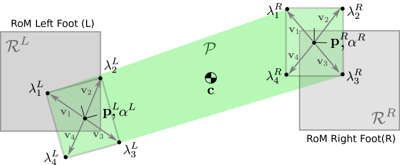
Figure 3: Top down view of a biped for both feet in contact at $\mathbf{p}^{R},\mathbf{p}^{L}\in\mathcal{R}$ inside the range of motion $\mathcal{R}$ (gray), which moves with the CoM position. For square feet with corners $\mathbf{v}_{v}$, rotated by $\alpha$, the support area is shown by $\mathcal{P}$ (light green area). This is the area to which the CoP $\mathbf{u}$ is constrained. If the biped controls its CoP to lie on the tip of the right foot, the corresponding corner carries all the load ($\lambda^{R}_{1}=1.0$), while the other seven lambdas are zero. In case of point-feet the support area is simply a straight line between $\mathbf{p}^{R}$ and $\mathbf{p}^{L}$.

III-C Center of Pressure Motion

To represent the continuous CoP trajectory, we parameterize it through the load carried by each endeffector. This parametrization is used to formulate a novel convexity constraint based on vertices instead of hyperplanes. Finally this section introduces a cost that keeps the CoP from marginally stable regions and improves robustness of the motion.

III-C1 CoP Parametrization

The CoP $\mathbf{u}(t)$ is not parametrized by polynomial coefficients or discrete points, but by the relative load each corner of each foot is carrying. This load is given by

$$\begin{split}\boldsymbol{\lambda}(t)&=\begin{bmatrix}\boldsymbol{\lambda}^{1}(t),\dots,\boldsymbol{\lambda}^{n_{f}}(t)\end{bmatrix}^{T},\\ \text{where }\boldsymbol{\lambda}^{f}(t)&=\begin{bmatrix}\lambda_{1}^{f}(t),\dots,\lambda^{f}_{n_{v}}(t)\end{bmatrix}\in\left[0,1\right]^{n_{v}}.\end{split}$$ (16)

${n_{v}}$ represents the number of vertices/corners of foot $f$. For the square foot in Fig. 3, four lambda values represent one foot and distribute the load amongst the corners. These multipliers represent the percentage of vertical force that each foot is carrying, e.g. $|\!|\boldsymbol{\lambda}^{f}(t)|\!|_{1}=0.9$ implies that leg $f$ is carrying 90% of the weight of the robot at time $t$. Using these values, the CoP is parameterized by

$$\mathbf{u}(t)=\sum_{f=1}^{n_{f}}\sum_{v=1}^{{n_{v}}}\lambda_{v}^{f}(t)(\mathbf{p}^{f}(t)+\mathbf{R}(\alpha^{f}(t))\mathbf{v}_{v}),$$ (17)

where $\mathbf{R}(\alpha^{f})\in\mathbb{R}^{2\times 2}$ represents the rotation matrix corresponding to the optimized rotation $\alpha^{f}$ of foot $f$ (13). $\mathbf{v}_{v}$ represents the fixed position (depending on the foot geometry) of corner $v$ of the foot expressed in the foot frame. For a point-foot robot with ${\mathbf{v}_{v}\!=\!\mathbf{0}}$, (17) simplifies to $\mathbf{u}=\sum_{f=1}^{n_{f}}\lambda^{f}\mathbf{p}^{f}$.

We represent $\boldsymbol{\lambda}(t)$ for the duration of the motion by piecewise-constant values $\boldsymbol{\lambda}_{i}=\boldsymbol{\lambda}(t_{i})$ discretized every $20\text{\,}\mathrm{m}\mathrm{s}$, resulting in $n_{u}$ nodes. Therefore the CoP $\mathbf{u}$ can be fully parameterized by $\mathbf{w}_{p}$ and the additional NLP decision variables

$$\mathbf{w}_{u}=\begin{bmatrix}\boldsymbol{\lambda}_{1},\dots,\boldsymbol{\lambda}_{n_{u}}\end{bmatrix}.$$ (18)

III-C2 Unilateral Forces Constraint

We represent the essential input constraint (6), which ensures that only physically feasible forces inside the convex hull of the contacts are generated, for $i=1,\dots,n_{u}$ as

$$\left\lVert\boldsymbol{\lambda}_{i}\right\rVert_{1} =1,$$ (19a)

$$0\leq\lambda_{v}^{f}[t_{i}] \leq c^{f}[t_{i}],$$ (19b)

where $c^{f}\,{\in}\,\{0,1\}\,{\in}\,\mathbb{Z}$ is the indicator if foot $f$ is in contact. The constraints (17) and (19a) allow $\mathbf{u}$ to be located anywhere inside the convex hull of the vertices of the current foot positions, independent of whether they are in contact. However, since only feet in contact can actually carry load, (19b) enforces that a leg that is swinging (${c^{f}\!=\!0}$) must have all the corners of its foot unloaded. These constraints together ensure that the CoP lies inside the green area shown in Fig. 3.

III-C3 Robust Walking Cost

To keep the CoP away from the edges of the support-area we could constrain $\lambda_{v}^{f}$ of each leg in stance to be greater than a threshold, causing these legs in contact to never be unloaded. This conceptually corresponds to previous approaches that heuristically shrink support areas and thereby reduce the solution-space for all situations. We propose a cost that has similar effect, but still permits the solver to use the limits of the space if necessary.

The most robust state to be in, is when the weight of the robot is equally distributed amongst all the corners in contact, so

$$\lambda^{f*}_{v}(t)=\frac{c^{f}(t)}{n_{v}(t)},$$ (20)

where $n_{v}(t)={n_{v}}\sum_{f=1}^{{n_{f}}}c^{f}(t)$ is the total number of vertices in contact at time $t$, predefined by the contact sequence $c(t)$. This results in the CoP to be located in the center of the support areas. The deviation of the input values from the optimal values $\lambda^{*}$ over the entire discretized trajectory (18) is then given by

$$J_{\lambda}(\mathbf{w}_{u})=\sum_{i=1}^{n_{u}}\left\lVert\boldsymbol{\lambda}_{i}-\boldsymbol{\lambda}^{*}_{i}\right\rVert_{2}^{2}.$$ (21)

For a support triangle (${\lambda^{f*}_{v}\!=\!\frac{1}{3}}$) this cost tries to keep the CoP in the center and for a line (${\lambda^{f*}_{v}\!=\!\frac{1}{2}}$) in the middle. For quadruped walking motions this formulation generates a smooth transition of the CoP between diagonally opposite swing-legs, while still staying away from the edges of support-areas whenever possible.

IV Tracking the Motion

The motion optimization part of our approach is largely robot independent. The only robot specific information needed to run the framework are the robot height, the number of feet, their geometry and their kinematic range. For execution however, the optimized motion must be translated into joint torques $\boldsymbol{\tau}$ using a fully-body dynamics model. This section discusses this generation summarized by Fig. 4.

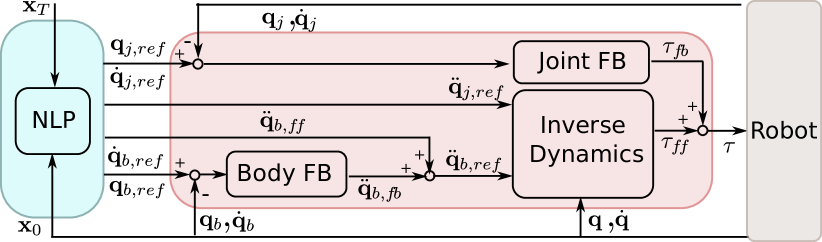
Figure 4: The controller that generates the required torques to execute a planned motion. Given the current state of the system $\mathbf{x}_{0}$ and a user defined goal state $\mathbf{x}_{T}$, the optimizer generates a reference motion. We augment this reference through a body feedback acceleration based on how much the body deviates from the desired motion. Inverse dynamics is used to generate the torques to achieve the reference base and joint accelerations.

IV-A Generating full-body reference accelerations

The 6–Degrees of Freedom (DoF) base pose is reconstructed using zero desired orientation (in Euler angles x,y,z), the optimized CoM motion $\mathbf{c}$ (assuming the geometric center of the base coincides with the CoM), and the constant base height $h$ as

$$\mathbf{q}_{b,ref}(t)=\begin{bmatrix}0&0&0&c_{x}(t)&c_{y}(t)&h\end{bmatrix}^{T}.$$

In order to cope with uncertainties it is essential to incorporate feedback into the control loop. We do this by adding an operational space PD-controller on the base that creates desired 6D base accelerations according to

$$\ddot{\mathbf{q}}_{b,ref}=\ddot{\mathbf{q}}_{b,f\!f}+K_{p}(\mathbf{q}_{b}-\mathbf{q}_{b,ref})+K_{d}(\dot{\mathbf{q}}_{b}-\dot{\mathbf{q}}_{b,ref}).$$

The derivate of the pose, the base twist $\dot{\mathbf{q}}_{b}\in\mathbb{R}^{6}$ represents the base angular and linear velocities and $\ddot{\mathbf{q}}_{b,f\!f}$ is the optimized CoM acceleration from the NLP. This controller modifies the planned body motion if the current state deviation from the reference state.

In order to obtain the desired joint accelerations that correspond to the planned Cartesian motion of the feet we can use the relationship $\ddot{\mathbf{p}}(t)=\mathbf{J}\ddot{\mathbf{q}}+\dot{\mathbf{J}}\dot{\mathbf{q}},$ where $\dot{\mathbf{q}},\ddot{\mathbf{q}}\in 6+n$ represent the full body state (base + joints) and $\mathbf{J}=\begin{bmatrix}\mathbf{J}_{b}&\mathbf{J}_{j}\end{bmatrix}\in\mathbb{R}^{3{n_{f}}\times(6+n)}$ the Jacobian that maps full-body velocities to linear foot velocities in world frame. Rearranging this equation, and using the Moore–Penrose pseudoinverse $\mathbf{J}_{j}^{+}$, gives us the reference joint acceleration

$$\ddot{\mathbf{q}}_{j,ref}=\mathbf{J}_{j}^{+}\left(\ddot{\mathbf{p}}-\dot{\mathbf{J}}\dot{\mathbf{q}}-\mathbf{J}_{b}\ddot{\mathbf{q}}_{b,ref}\right).$$ (22)

IV-B Inverse Dynamics

The inverse dynamics controller is responsible for generating required joint torques $\boldsymbol{\tau}$ to track the reference acceleration $\ddot{\mathbf{q}}_{ref}$, which is physically feasible based on the LIP model. This is done based on the rigid body dynamics model of the system, which depends on the joint torques, but also the unknown contact forces. To eliminate the contact forces from the equation, we project it into the space of joint torques by $\mathbf{P}=\mathbf{I}-\mathbf{J}_{c}^{+}\mathbf{J}_{c},$ where $\mathbf{J}^{T}_{c}$ is the contact Jacobian that maps Cartesian contact forces to joint torques [26, 27]. This allows us to solve for the required joint torques through

$$\boldsymbol{\tau}=(\mathbf{P}\mathbf{S}^{T})^{+}\ \mathbf{P}(\mathbf{M}\ddot{\mathbf{q}}_{ref}+\mathbf{C}),$$ (23)

where $\mathbf{M}$ is the joint space inertia matrix, $\mathbf{C}$ the effect of Coriolis forces on the joint torques and $\mathbf{S}$ the selection matrix which prohibits from actuating the floating base state directly. We found it beneficial to also add a low-gain PD-controller on the joint position and velocities. This can mitigate the effects of dynamic modeling errors and force tracking imperfections.

V Results

We demonstrate the performance of this approach on the hydraulically actuated quadruped robot HyQ [28]. The robot weighs approximately $80\text{\,}\mathrm{kg}$, moves at a height of about $0.6\text{\,}\mathrm{m}$ and is torque controlled. Base estimation [29] is performed on-board, fusing Inertial Measurement Unit (IMU) and joint encoder values. Torque tracking is performed at $1000\text{\,}\mathrm{Hz}$, while the reference position, velocity and torque set-points are provided at $250\text{\,}\mathrm{Hz}$. The C++ dynamics model is generated by [30].

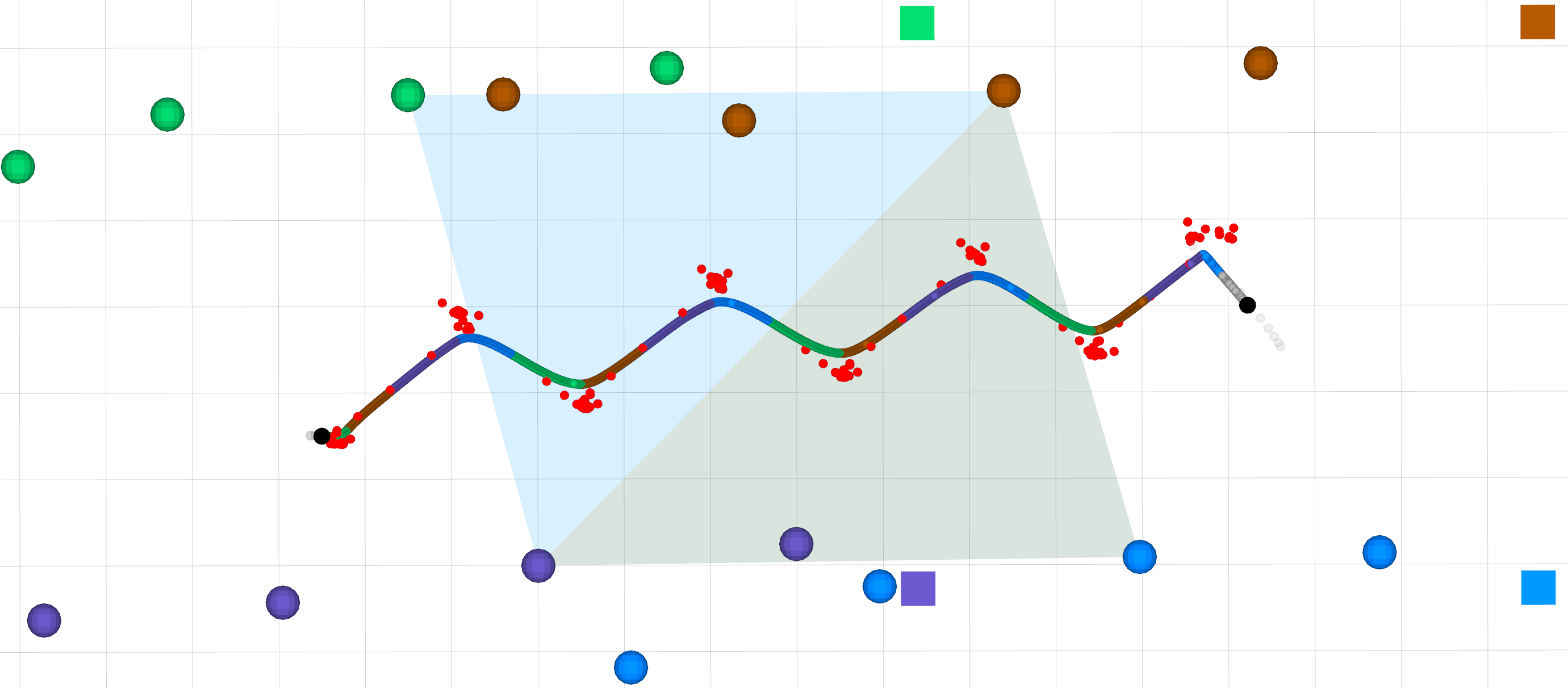
(a) Quadruped Walk: swinging one leg at a time.

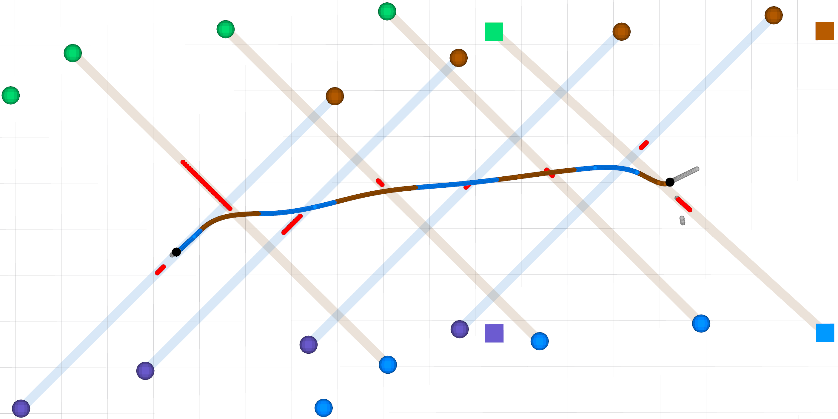
(b) Quadruped Trot: swinging diagonally opposite legs.

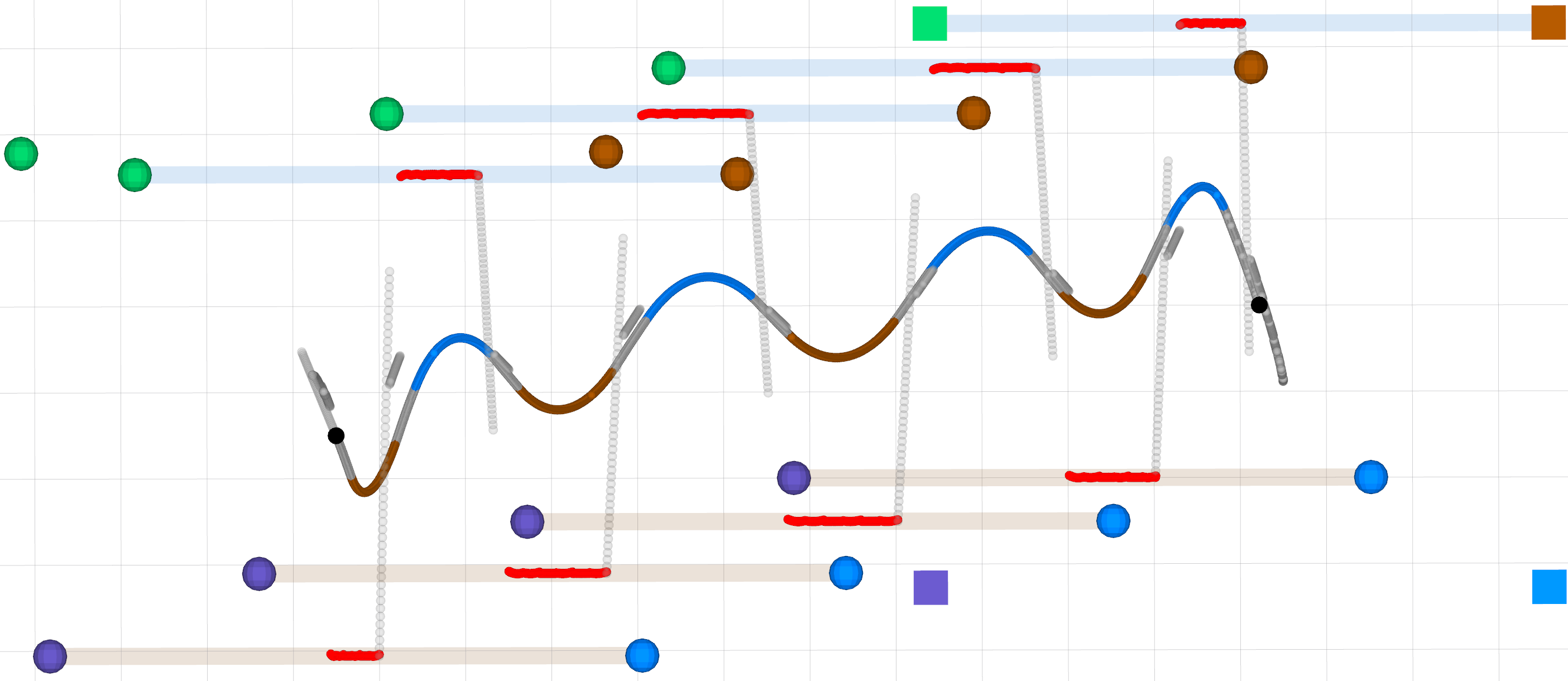
(c) Quadruped Pace: swinging left, then right legs.

(d) Quadruped Bound: swinging front, then hind legs.

Figure 5: Top down view of the generated motions for a quadruped robot moving from left to right, swinging the legs $f$ left-hind (blue), left-front (purple), right-hind (brown), right-front (green) in the sequence shown. The initial stance is shown by the squares, the optimized steps by the circles. The CoM motion $\mathbf{p}^{f}(t)$ is shown by the solid line, where the color corresponds to the swingleg(s) at that moment. If all legs are in contact during, the motion and corresponding CoP is shown in gray. The support area for each phase is shown by the transparent areas. The optimized CoP positions $\mathbf{u}(t)$ that drive the system are shown in red and always lie inside the support area.

V-A Discussion of generated motions

This section analyses the different motions generated by changing the sequence and timings of contacts $c(t)$. There is no high-level footstep planner; the footholds are chosen by the optimizer to enable the body to reach a user defined goal state $\mathbf{x}_{T}$. The results where obtained using C++ code interfaced with Interior Point Method (Ipopt [31]) or Sequential Quadratic Programming (Snopt [32]) solvers on an Intel Core i7/$2.8\text{\,}\mathrm{G}\mathrm{H}\mathrm{z}$ Quadcore laptop. The Jacobians of the constraint and the gradient of the cost function are provided to the solver analytically, which is important for performance. We initialize the decision variables $\mathbf{w}$ with the quadruped standing in default stance for a given duration. The shown motions correspond to the first columns (e.g. 16 steps) in Table I. The reader is encouraged to view the video at https://youtu.be/5WLeQMBuv30, as it very intuitively demonstrates the performance of this approach. Apart from the basic gaits, the video shows the capability of the framework to generate gradual transitions between them, bipedal walking, limping and push-recovery.

V-A1 Walk

Fig. 5(a) shows a walk of multiple steps, with the two support areas highlighted for swinging RF$\to$LH. The effect of the cost term $J_{\lambda}$ is clearly visible, as the CoP is accumulated away from the support area borders by left-right swaying of the body. Only when switching diagonally opposite legs the CoP lies briefly at the marginally stable border, but then immediately shifts to a more conservative location. Without the cost term, the CoM motion is a straight line between $\mathbf{x}_{0}$ and $\mathbf{x}_{T}$, causing the real system to fail.

V-A2 Trot

Fig. 5(b) shows a completely different pattern of support areas and CoP distribution. During trotting only line-contacts exist, so the possible places to generate the CoP is extremely restricted compared to walking. Notice how the CoP lies close to the CoM trajectory during the middle of the motion, but deviates quite large back/forward during the start/end of the motion (e.g. the robot pushing off from the right-front (green) leg in the second to last step). This is because the distance between the CoP and the CoM generates the acceleration necessary for starting and stopping, whereas in the middle the robot is moving with nearly constant velocity.

V-A3 Pace/Bound/Biped Walk

Specifying legs on the same side to be in contact, with a short four-leg transition period between them produces the motion shown in Fig. 5(c). This can also be viewed as biped walking with line-feet (e.g. skis), with the constraint enforced also during the double-stance phase. The first observation is the sideways swaying motion of the CoM. This is necessary because the support areas do not intersect (as in the trot) the CoM trajectory. Since the CoP always lies inside these left and right support areas, they will accelerate the body away from that side until the next step, which then reverses the motion. We found that the LIP model with fixed zero body orientation does not describe such a motion very well, as the inherent rotation (rolling) of the body is not taken into account. In order to also demonstrate these motions on hardware, the LIP model must be extended by the angular body motion. Specifying the front and hind legs to alternate between contact generates a bound Fig. 5(d). The lateral shifting motion of the pace is now transformed to a forward backward motion of the CoM due to support areas. In case of an omni directional robot a bounding gait can simply be considered a side-ways pace.

TABLE I: Specs of the NLP for 16- and 4-step motions

	(16 steps, $1\text{\,}\mathrm{m}$) $|$ (4 steps, $0.2\text{\,}\mathrm{m}$)
	Walk	Trot	Pace	Bound
Horizon $T$ [s]	6.4 $|$ 1.6	2.4 $|$ 0.6	3.2 $|$ 0.8	3.2 $|$ 0.8
Variables [-]	646 $|$ 202	387 $|$ 162	1868 $|$ 728	1868 $|$ 728
Constraints [-]	850 $|$ 270	548 $|$ 255	2331 $|$ 939	2331 $|$ 939
$t_{k+1}-t_{k}$ [s]	0.1	0.05	0.02	0.02
Cost term	$J_{\lambda}$	-	-	-
Time Ipopt [s]	0.25 $|$ 0.06	0.02 $|$ 0.01	0.21 $|$ 0.12	0.17 $|$ 0.04
Time Snopt [s]	0.35 $|$ 0.04	0.04 $|$ 0.01	0.54 $|$ 0.18	0.42 $|$ 0.29

VI Conclusion

This paper presented a TO formulation using vertex-based support-area constraints, which enables the generation of a variety of motions for which previously separate methods were necessary. In the future, more decision variables (e.g. contact schedule, body orientation, foothold height for uneven terrain), constraints (e.g. friction cone, obstacles) and more sophisticated dynamic models can be incorporated into this formulation. Additionally, we plan to utilize the speed of the optimization for Model Predictive Control (MPC).

-A Derivation of Capture Point

Consider the differential equation describing a LIP (linear, constant coefficients, second order) in x-direction

$$\ddot{c}(t)-\frac{g}{h}c(t)=-\frac{g}{h}u$$ (24)

The general solution to the homogeneous part of the equation can be construct by the Ansatz $c(t)=e^{\alpha t}$ which leads to the characteristic equation $\alpha^{2}e^{\alpha t}-\frac{g}{h}e^{\alpha t}=0,$ resulting in $\alpha=\pm\sqrt{\frac{g}{h}}.$ Assuming constant input $u_{0}$ leads to the partial solution $c_{p}(t)=u_{0}$, and the space of solutions for the entire ODE is given by

$$c(t)=\beta_{1}e^{\alpha t}+\beta_{2}e^{-\alpha t}+u_{0}$$ (25)

where $\beta_{1},\beta_{2}\in\mathbb{R}$ are the free parameters describing the motion. Imposing the initial position $c(0)=\beta_{1}+\beta_{2}+u_{0}\overset{!}{=}c_{0}$ and velocity $\dot{c}(0)=\alpha\beta_{1}-\alpha\beta_{2}\overset{!}{=}\dot{c}_{0}$ we obtain

$$\beta_{1,2}=\frac{1}{2}(c_{0}\pm\frac{\dot{c}_{0}}{\alpha}-u_{0}).$$ (26)

As $t\to\infty$ we require the velocity to remain at zero (pendulum at rest). Since $\lim_{t\to\infty}e^{-\alpha t}=0$, and $\alpha\neq 0$ we have

$$\lim_{t\to\infty}\dot{c}_{x}(t) =\alpha\beta_{1}\lim_{t\to\infty}e^{\alpha t}\overset{!}{=}0\quad\Leftrightarrow\quad\beta_{1}=0$$ (27)

$$\Rightarrow u_{0}=c_{0}+\frac{h}{g}\dot{c}_{0},$$ (28)

which is known as the one-step Capture Point originally derived in [14].

-B Dynamic Constraint

The system dynamics constraint (11) enforced through $\ddot{\mathbf{c}}[t]=\mathbf{f}_{2}(\mathbf{x}[t],\mathbf{u}[t])$, with the local polynomial time ${\underaccent{\bar}{t}\!=\!(t-t_{k})}$, are formulated as

$$\ddot{\mathbf{c}}[t]=\sum_{i=2}^{4}i(i-1)\mathbf{a}_{k,i}\underaccent{\bar}{t}^{i-2}=\frac{g}{h}(\mathbf{c}(t)-\mathbf{u}(t))$$

$$\Leftrightarrow \sum_{i=2}^{4}\mathbf{a}_{k,i}\underaccent{\bar}{t}^{i-2}\left(i(i-1)-\frac{g}{h}\underaccent{\bar}{t}^{2}\right)=\frac{g}{h}(\mathbf{a}_{k,0}+\mathbf{a}_{k,1}\underaccent{\bar}{t}-\mathbf{u}(t)).$$

References

- [1] G. Schultz and K. Mombaur, “Modeling and optimal control of human-like running,” IEEE/ASME Transactions on Mechatronics, vol. 15, no. 5, pp. 783–792, 2010.
- [2] H. Dai, A. Valenzuela, and R. Tedrake, “Whole-body Motion Planning with Simple Dynamics and Full Kinematics,” IEEE-RAS International Conference on Humanoid Robots, 2015.
- [3] M. Posa, C. Cantu, and R. Tedrake, “A direct method for trajectory optimization of rigid bodies through contact,” The International Journal of Robotics Research, vol. 33, no. 1, pp. 69–81, 2013.
- [4] I. Mordatch, E. Todorov, and Z. Popović, “Discovery of complex behaviors through contact-invariant optimization,” ACM Transactions on Graphics, vol. 31, no. 4, pp. 1–8, 2012.
- [5] M. Posa, S. Kuindersma, and R. Tedrake, “Optimization and stabilization of trajectories for constrained dynamical systems,” Proceedings - IEEE International Conference on Robotics and Automation, vol. 2016-June, no. 724454, pp. 1366–1373, 2016.
- [6] M. Neunert, F. Farshidian, A. W. Winkler, and J. Buchli, “Trajectory optimization through contacts and automatic gait discovery for quadrupeds,” to appear in IEEE Robotics and Automation Letters (RA-L), 2017.
- [7] D. Pardo, M. Neunert, A. W. Winkler, and J. Buchli, “Hybrid direct collocation and control in the constraint-consistent subspace for dynamic legged robot-legged locomotion,” RSS Science and Systems Conference, 2017.
- [8] S. Coros, A. Karpathy, B. Jones, L. Reveret, and M. van de Panne, “Locomotion skills for simulated quadrupeds,” ACM SIGGRAPH, p. 1, 2011.
- [9] M. Vukobratović and B. Borovac, “Zero-moment point - thirty five years of its life,” International Journal of Humanoid Robotics, vol. 1, no. 01, pp. 157–173, 2004.
- [10] S. Kajita, F. Kanehiro, K. Kaneko, K. Fujiwara, K. Harada, K. Yokoi, and H. Hirukawa, “Biped walking pattern generation by using preview control of zero-moment point,” IEEE International Conference on Robotics and Automation, pp. 1620–1626, 2003.
- [11] M. Kalakrishnan, J. Buchli, P. Pastor, M. Mistry, and S. Schaal, “Fast, robust quadruped locomotion over challenging terrain,” IEEE International Conference on Robotics and Automation, pp. 2665–2670, 2010.
- [12] J. Z. Kolter, M. P. Rodgers, and A. Y. Ng, “A control architecture for quadruped locomotion over rough terrain,” IEEE International Conference on Robotics and Automation, pp. 811–818, 2008.
- [13] J. Carpentier, S. Tonneau, M. Naveau, O. Stasse, and N. Mansard, “A versatile and efficient pattern generator for generalized legged locomotion,” IEEE International Conference on Robotics and Automation, vol. 2016-June, no. 3, pp. 3555–3561, 2016.
- [14] J. Pratt, J. Carff, S. Drakunov, and A. Goswami, “Capture point: A step toward humanoid push recovery,” in IEEE-RAS International Conference on Humanoid Robots, 2006, pp. 200–207.
- [15] C. Gehring, S. Coros, M. Hutter, M. Bloesch, M. A. Hoepflinger, and R. Siegwart, “Control of dynamic gaits for a quadrupedal robot,” Proceedings - IEEE International Conference on Robotics and Automation, pp. 3287–3292, 2013.
- [16] V. Barasuol, J. Buchli, C. Semini, M. Frigerio, E. R. De Pieri, and D. G. Caldwell, “A reactive controller framework for quadrupedal locomotion on challenging terrain,” IEEE International Conference on Robotics and Automation, pp. 2554–2561, 2013.
- [17] I. Mordatch, M. de Lasa, and A. Hertzmann, “Robust physics-based locomotion using low-dimensional planning,” ACM Transactions on Graphics, vol. 29, no. 4, p. 1, 2010.
- [18] B. J. Stephens and C. G. Atkeson, “Push recovery by stepping for humanoid robots with force controlled joints,” in IEEE-RAS International Conference on Humanoid Robots, Humanoids 2010, 2010, pp. 52–59.
- [19] H. Diedam, D. Dimitrov, P.-b. Wieber, K. Mombaur, and M. Diehl, “Online Walking Gait Generation with Adaptive Foot Positioning through Linear Model Predictive Control,” IEEE International Conference on Intelligent Robots and Systems, 2009.
- [20] A. Herdt, N. Perrin, and P. B. Wieber, “Walking without thinking about it,” IEEE International Conference on Intelligent Robots and Systems, pp. 190–195, 2010.
- [21] M. Naveau, M. Kudruss, O. Stasse, C. Kirches, K. Mombaur, and P. Souères, “A ReactiveWalking Pattern Generator Based on Nonlinear Model Predictive Control,” IEEE Robotics and Automation Letters, vol. 2, no. 1, pp. 10–17, 2017.
- [22] A. W. Winkler, F. Farshidian, M. Neunert, D. Pardo, and J. Buchli, “Online walking motion and foothold optimization for quadruped locomotion,” in IEEE International Conference on Robotics and Automation, 2017.
- [23] D. Serra, C. Brasseur, A. Sherikov, D. Dimitrov, and P.-b. Wieber, “A Newton method with always feasible iterates for Nonlinear Model Predictive Control of walking in a multi-contact situation,” 2016 IEEE-RAS International Conference on Humanoid Robots (Humanoids 2016), no. 1, pp. 6–11, 2016.
- [24] M. Diehl, H. G. Bock, H. Diedam, and P. B. Wieber, “Fast direct multiple shooting algorithms for optimal robot control,” Lecture Notes in Control and Information Sciences, vol. 340, pp. 65–93, 2006.
- [25] C. Hargraves and S. Paris, “Direct trajectory optimization using nonlinear programming and collocation,” Journal of Guidance, Control, and Dynamics, 1987.
- [26] F. Aghili, “A unified approach for inverse and direct dynamics of constrained multibody systems based on linear projection operator: Applications to control and simulation,” IEEE Transactions on Robotics, vol. 21, no. 5, pp. 834–849, 2005.
- [27] M. Mistry, J. Buchli, and S. Schaal, “Inverse dynamics control of floating base systems using orthogonal decomposition,” IEEE International Conference on Robotics and Automation, no. 3, pp. 3406–3412, 2010.
- [28] C. Semini, “HyQ - Design and development of a hydraulically actuated quadruped robot,” Ph.D. dissertation, Istituto Italiano di Tecnologia, 2010.
- [29] M. Bloesch, M. Hutter, M. A. Hoepflinger, S. Leutenegger, C. Gehring, C. D. Remy, and R. Siegwart, “State Estimation for Legged Robots - Consistent Fusion of Leg Kinematics and IMU,” Robotics: Science and Systems, p. 2005, 2012.
- [30] M. Frigerio, J. Buchli, D. G. Caldwell, and C. Semini, “RobCoGen : a code generator for efficient kinematics and dynamics of articulated robots , based on Domain Specific Languages,” Journal of Software Engineering for Robotics, vol. 7, no. July, pp. 36–54, 2016.
- [31] A. Waechter and L. T. Biegler, On the implementation of an interior-point filter line-search algorithm for large-scale nonlinear programming, 2006, vol. 106, no. 1.
- [32] P. E. Gill, W. Murray, and M. A. Saunders, “SNOPT: An SQP Algorithm for Large-Scale Constrained Optimization,” pp. 979–1006, 2002.