Effective Metrics for Multi-Robot Motion-Planning

Abstract

We study the effectiveness of metrics for Multi-Robot Motion-Planning (MRMP) when using RRT-style sampling-based planners. These metrics play the crucial role of determining the nearest neighbors of configurations and in that they regulate the connectivity of the underlying roadmaps produced by the planners and other properties like the quality of solution paths. After screening over a dozen different metrics we focus on the five most promising ones—two more traditional metrics, and three novel ones which we propose here, adapted from the domain of shape-matching. In addition to the novel multi-robot metrics, a central contribution of this work are tools to analyze and predict the effectiveness of metrics in the MRMP context. We identify a suite of possible substructures in the configuration space, for which it is fairly easy (i) to define a so-called natural distance, which allows us to predict the performance of a metric. This is done by comparing the distribution of its values for sampled pairs of configurations to the distribution induced by the natural distance; (ii) to define equivalence classes of configurations and test how well a metric covers the different classes. We provide experiments that attest to the ability of our tools to predict the effectiveness of metrics: those metrics that qualify in the analysis yield higher success rate of the planner with fewer vertices in the roadmap. We also show how combining several metrics together leads to better results (success rate and size of roadmap) than using a single metric.

1 Introduction

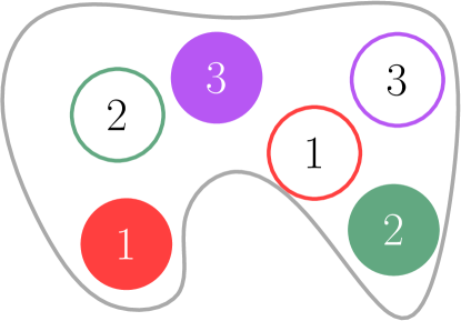
Figure 1: An example of an MRMP instance with $m=3$ translating discs. The full discs represent the start configurations and the empty discs represent the goal configurations. Each disc needs to move from its start configuration to its goal configuration without hitting the boundary of the workspace nor its fellow robots.

Multi-robot motion-planning (MRMP) is the problem of planning the motion of a fleet of robots from given start to goal configurations, while avoiding collisions with obstacles and with each other. See Figure 1 for a simple illustration. It is a natural extension of the standard single-robot motion-planning problem. MRMP is notoriously challenging, both from the theoretical and practical standpoint, as it entails a prohibitively-large search space, which accounts for a multitude of robot-obstacle and robot-robot interactions.

Sampling-based planners have proven to be effective in challenging settings of the single-robot case, and a number of such planners have been proposed for MRMP (Dobson et al., 2017; Solovey et al., 2016; Švestka and Overmars, 1998; Wagner and Choset, 2015). Sampling-based planners attempt to capture the connectivity of the free space by sampling random configurations and connecting nearby configurations by simple collision-free paths. In order to measure similarity, or “closeness”, between a given pair of configurations a metric is employed by the algorithm. The choice of metric has a tremendous effect on the performance of planners and the quality of the returned solutions (see Section 2 for further discussion about metrics that are tailored for various robotic systems). Nevertheless, no specialized metrics for multi-robot systems have been proposed, to the best of our knowledge.

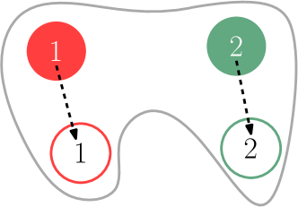
(a) “Easy” to-connect configurations

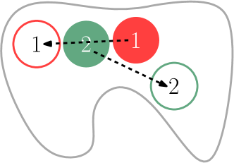
(b) “Hard” to-connect configurations

Figure 2: Example for the setting of two disc robots, drawn in red and green, respectively. Full discs represent start configurations, and empty discs represent goal configurations. Since it is easier to connect the configurations in (a) when compared to the configurations in (b), the distance in (a) should be smaller than the distance in (b).

A common approach (see  (Choset et al., 2005, pp. 210)) states that the metric should reflect how difficult it is to plan a path between two configurations. See Figure 2 for an illustration. Nowadays, a common metric for multi-robot systems is defined as a sum of metric values for single robots ((Plaku and Kavraki, 2006; Solovey et al., 2016), and in fact this is the default in OMPL (Open Motion Planning Library) (Sucan et al., 2012)), i.e., the sum of distances induced by each of the robots separately. We denote this metric by $\Sigma L_{2}$ (to be formally defined in Section 4). This metric does not always adequately express distance in the configuration space ($\mathcal{C}$-space) because it does not account for interactions between different robots. A simple example is shown in Figure 3.

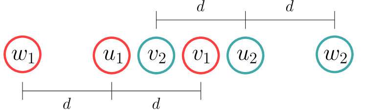
Figure 3: Example of $\Sigma L_{2}$ for the setting of $m=2$ disc robots in the plane. The red discs, centered in $u_{1},v_{1},w_{1}$ represent possible positions for the first robot, whereas the green discs, centered in $u_{2},v_{2},w_{2}$, represent possible positions for the second robot. We set the positions in the following manner: $\|u_{1}-v_{1}\|_{2}=\|u_{1}-w_{1}\|_{2},\|u_{2}-v_{2}\|_{2}=\|u_{2}-w_{2}\|_{2}$. $U=(u_{1},u_{2}),V=(v_{1},v_{2}),W=(w_{1},w_{2})$ represent three simultaneous placements of the two robots. While $\Sigma L_{2}\left(U,V\right)=\Sigma L_{2}\left(U,W\right)$, it is intuitive that it is easier to connect $U$ to $W$ rather than to $V$. This example hints that $\Sigma L_{2}$ may not be suitable for all cases as it fails to capture robot-robot interaction.

1.1 Contribution

We study the effectiveness of metrics for MRMP when using RRT-style sampling-based planners. These metrics play the crucial role of determining the nearest neighbors of configurations and in that they regulate the connectivity of the underlying roadmaps produced by the planners and other properties like the quality of solution paths. After screening over a dozen different metrics we focus on the five most promising ones—two more traditional metrics, and three novel ones which we propose here, adapted from the domain of shape-matching. In addition to the novel multi-robot metrics, a central contribution of this work are tools to analyze and predict the effectiveness of metrics in the MRMP context. We identify a suite of possible substructures in the configuration space, for which it is fairly easy (i) to define a so-called natural distance, which allows us to predict the performance of a metric. This is done by comparing the distribution of its values for sampled pairs of configurations to the distribution induced by the natural distance; (ii) to define equivalence classes of configurations and test how well a metric covers the different classes. We provide experiments that attest to the ability of our tools to predict the effectiveness of metrics: those metrics that qualify in the analysis yield higher success rate of the planner with fewer vertices in the roadmap. We also show how combining several metrics together leads to better results (success rate and size of roadmap) than using a single metric.

1.2 Organization

The organization of this paper is as follows. In Section 2 we review related work. In Section 3 we describe the early phase of our investigation, where we tested a large number of metrics with different planners, and explain why we chose the metrics and planner on which we focus in the sequel. In Section 4 we formally define five metrics which will be discussed later. In Sections 5 and 6 we present methods for analyzing the proposed metrics using identification of substructures arising in MRMP. In Section 7 we provide experimental results allowing us to compare the utility of the metrics. In Section 8 we extend the metrics for robotic systems other than those we discuss earlier. Finally, in Section 9 we outline possible future work.

2 Related Work

We start this section with work related to multi-robot motion planning (MRMP). Then, we proceed to discuss metrics in the context of robotics and beyond. We assume some familiarity with basic concepts of sampling-based motion planning (see, e.g., Choset et al. (2005); Halperin et al. (2016); LaValle (2006)).

2.1 Multi-robot motion-planning

Initial work on MRMP focused on exact methods for solving the problem instance. Schwartz and Sharir (1983) consider the case of disc robots operating in an environment cluttered with polygonal obstacles. Their algorithm runs in time polynomial in the obstacles’ complexity, but exponential in the number of robots. Several works address the case when the number of robots is bounded. Aronov et al. (1999) present a technique that reduces the complexity of the problem for two or three robots.Sharir and Sifrony (1991) propose an approach to coordinate the motion between two robots of various types, i.e., not necessarily translating robots.

Hopcroft et al. (1984) and Hopcroft and Wilfong (1986) prove that MRMP is PSPACE-hard even when the robots are rectangular and operate in a rectangular region. Later, Hearn and Demaine (2005, 2009) extend the result to rectangles of size $1\times 2$ and $2\times 1$. The problem is strongly NP-hard also when the robots are translating discs (Spirakis and Yap, 1984). The proof in (Spirakis and Yap, 1984) makes use of robots that differ in their size. In a recent result (Solovey and Halperin, 2016), the setting of unit-square robots and polygonal obstacles is considered. The problem is proven to be PSPACE-hard. The result holds even in case that all the robots are identical and indistinguishable (namely, in the unlabeled setting). In addition to the aforementioned results, system dynamics can introduce additional complications to the problem (Johnson, 2016).

The unlabeled variant of the problem was introduced by Kloder and Hutchinson (2005) who describe a sampling-based planner for the problem. Although this problem is hard in general, under some simplifying assumptions it can be solved in polynomial time as function of the number of robots and the complexity of the workspace environment. For disc-shape robots, under some assumptions on the free space and the separation between initial and goal configurations, it is possible to find a solution in polynomial time (Turpin et al., 2014). Furthermore, the obtained solution is optimal with respect to the longest distance traveled by any one robot. Adler et al. (2015) describe a more efficient algorithm, which guarantees to find a solution, but not necessarily the best one. Using similar conditions a nearly optimal solution (with respect to the sum of path lengths) can be found in polynomial time (Solovey et al., 2015). Finally, we mention that the $k$-color generalization, where the robots are partitioned into $k$ groups and the robots in each group are indistinguishable, has been studied using a sampling-based approach (Solovey and Halperin, 2014).

Approaches for solving MRMP can be roughly subdivided into two types: coupled and decoupled. In the latter approach (see, e.g., Bareiss and van den Berg (2015); Leroy et al. (1999); van den Berg and Overmars (2005)), a path or an initial plan are found for each robot separately, and then the paths are coordinated with each other. Although this approach is less sensitive to the number of robots, when compared with the coupled approach, it gives no completeness guarantees.

The coupled approach usually treats the entire system as a single robot, for which the number of degrees of freedom (DOFs) is equal to the sum of the number of DOFs of the individual robots in the system. This approach usually comes with stronger theoretical guarantees such as completeness (Kloder and Hutchinson, 2005; Salzman et al., 2015; Sanchez and Latombe, 2002; Solovey and Halperin, 2014; Solovey et al., 2016) or even optimality (Wagner and Choset, 2015; Dobson et al., 2017) of the returned solutions. However, due to the computational hardness of MRMP (Hearn and Demaine, 2005; Hopcroft et al., 1984; Johnson, 2016; Solovey and Halperin, 2016; Spirakis and Yap, 1984), coupled techniques do not scale well with the increase in the number of robots.

2.2 Metrics

The choice of a metric for nearest-neighbors queries in a sampling-based planner can be crucial. Amato et al. (2000) were the first to study the effect of a metric on sampling-based planners. They consider PRM (Kavraki et al., 1996) as the planner and define effectiveness as the number of discovered edges in the roadmap. They compare effectiveness of some variants of the Euclidean metric in settings that involve translation and rotation of a single robot. Kuffner (2004) considers metrics for rigid-body motion and proposes an interpolation between the rotation component and the translation component.

Extensive research has been carried out in order to find suitable metrics for other settings of motion planning, such as robots with differential constraints (Bharatheesha et al., 2014; Boeuf et al., 2015; LaValle and Kuffner, 1999; Palmieri and Arras, 2015).

Pamecha et al. (1997) analyze metrics for systems with a single robot consisting of multiple modules that must stay in touch with each other (multi-module systems). Though any module can be thought of as a robot, the system restrictions are that modules are only allowed to move on a grid, and must stay in contact in order to form a metamorphic robot. Hence, their results are not straightforward to extend to arbitrary multi-robot systems. Further analysis for multi-module systems can be found in Winkler et al. (2011) and Zykov et al. (2007).

Recent methods employ machine learning to develop metrics that are tailored to the specific motion-planning problem at hand. Ekenna et al. (2013) introduce a framework in which there is a candidate set of metrics, and the planner adaptively selects a metric on-the-fly. The selection may vary over time or between different regions of the workspace. This implies that a set of metrics, each suitable for a different setting, can be combined in order to solve more diverse settings that consist of smaller, specific, (sub)settings. Morales et al. (2004) have the same observation that different portions of the $\mathcal{C}$-space may behave differently. In our work we will also refer to the case where different metrics are more effective than others in different portions of the $\mathcal{C}$-space.

Estimating distances between sets of points is in broad use in shape matching (see the survey  (Veltkamp and Hagedoorn, 2001)). Such techniques (see, e.g., Belongie et al. (2002)) are concerned with estimating the distance between shapes and with finding a matching between shapes. Kendall (1984) provides a rigorous mathematical study of the subject, where point sets are mapped to high-dimensional points, on which distance measures can be more easily defined (see more details in Section 4).

Another area where distance between sets of points is of interest is graph drawing. Bridgeman and Tamassia (2000) list a large number of distance metrics between planar graphs. Some of the metrics give a significant weight to the relative order between the nodes, which is also the guideline for the metrics we propose in this paper. Lyons et al. (1998) address the same problem, and measure similarity based on both Euclidean distance and relative order between the nodes.

3 Initial Screening

We began our study by experimenting with four different planners, fifteen different metrics and variations of them. For planners we tried RRT-style and EST-style (Hsu et al., 1999) planners that are adapted to the multi-robot setting. We tested both single-tree and bi-directional variants of each algorithm. PRM-style planners cannot cope with the induced high-dimensional space. RRT-style planners showed much better success rate in solving MRMP problems when compared to EST-style planners. This is why the study continues henceforth with dRRT (Solovey et al., 2016)—an adaptation of RRT to the multi-robot setting, which can cope with a larger number of robots and more complicated tasks than RRT as-is. We mention that M* (Wagner and Choset, 2015), which is another sampling-based planner tailored for MRMP, is less relevant to our current discussion since it only employs metrics concerning individual robots.

For metrics, we began by following the common approach of choosing metrics that have high correlation with the failure rate of the local planner (Choset et al., 2005, pp. 210). Note that this is also the guideline behind using the swept volume and its approximations as a metric for rotating robots (Amato et al., 2000; Ekenna et al., 2013; Kuffner, 2004). It turns out that when using such metrics with RRT-style planners, the exploration of the $\mathcal{C}$-space is unbalanced— the explored configurations tend to have the robots separated from each other. The analogue for single-robot planning is exploration of configurations that tend to be far from obstacles, avoiding paths that go near the obstacles. This phenomenon is further discussed in Appendix B.

We continue with metrics that adapt geometric methods from the domain of shape-matching (Belongie et al., 2002; Goodman and Pollack, 1980, 1983; Kendall, 1984), including existing methods that are used for mismatch measure (Alt et al., 1988). We also used measures of similarities that are employed in the domain of graph-drawing (Bridgeman and Tamassia, 2000; Lyons et al., 1998).

Out of the fifteen tested metrics and their variations, we remained with the five most successful metrics that are described below in Section 4.

Finally, we mention that we experimented with several types of robots including planar ones that are allowed to translate and rotate. All the metrics in this paper can cope with such robots (see Section 8). However, we chose to conduct our final experiments and analyses with robots bound to translate in the plane, as it makes the presentation clearer. Moreover, we believe that the study of complex rigid-body motion (Kuffner, 2004) in the context of metrics is mostly orthogonal to our current efforts of incorporating multi-robot considerations into the metric. Robotic systems involving dynamics are outside the scope of this paper, and we leave their study for future work.

4 Metrics for Multi-Robot Motion-Planning

In this section we discuss the role of metrics in sampling-based MRMP. Then, we formally define the standard $\Sigma L_{2}$, $\max L_{2}$ metrics and introduce the metrics $\varepsilon_{2}$, $\varepsilon_{\infty}$, Ctd, which will be evaluated in Section 7.

We consider $m$ robots $r_{1},\ldots,r_{m}$ operating in a shared workspace. For simplicity we assume that the robots are identical in shape and function. The $\mathcal{C}$-space of each individual robot can be denoted by some $\mathcal{X}$. Note that we still distinguish between the different robots. We assume that each $r_{i}$ represents a translating disc in the plane, and so $\mathcal{X}=\mathbb{R}^{2}$. Denote the joint $\mathcal{C}$-space for the $m$ individual robots by $\mathcal{X}^{m}=\mathcal{X}\times\ldots\times\mathcal{X}$, i.e., a joint configuration $U=(u_{1},\ldots,u_{m})$ represents a set of configurations for the $m$ robots.

Our presentation focuses on translating disc robots, which are often encountered in practice as iRobots, TurtleBots, or as the bounding volume to more complex systems. However, we note that the metrics described below can be extended to more general settings of the problem, such as non-disc robots and 3D environments. See Section 8 for more details.

Sampling-based tools for single and multi-robot systems rely on metrics to measure similarity between configurations. Let $U,V,W$ be joint configurations of our multi-robot system. A metric in the context of MRMP is a distance function $\mathrm{d}\!:\mathcal{X}^{m}\times\mathcal{X}^{m}\rightarrow\left[0,\infty\right)$, which satisfies the five properties:

1. non-negativity: $\mathrm{d}\!\left(U,V\right)\geq 0$;

2. identity: $\mathrm{d}\!\left(U,U\right)=0$;

3. identity of indiscernibles: $\mathrm{d}\!\left(U,V\right)=\!0\Rightarrow U=V$;

4. symmetry: $\mathrm{d}\!\left(U,V\right)=\mathrm{d}\!\left(V,U\right)$;

5. triangle inequality: $\mathrm{d}\!\left(U,W\right)\leq\mathrm{d}\!\left(U,V\right)+\mathrm{d}\!\left(V,W\right)$.

Efficient nearest-neighbors data structures usually do not rely on property c (see, e.g., (Brin, 1995; Chávez et al., 2001; Ciaccia et al., 1997)), and so can be applied to pseudometrics, which satisfy properties a, b, d and e. We extend the discussion also to pseudosemimetrics which are functions that satisfy only properties a, b, and  d. In that case, we cannot use sophisticated data structures that rely on the triangle inequality. For simplicity, from now on we will refer to any pseudosemimetric as a metric.

Standard metrics. The following two metrics are simple extensions of single-robot metrics to the multi-robot setting. Let $L$ be a single-robot metric $L:\mathcal{X}\times\mathcal{X}\rightarrow\left[0,\infty\right)$. For any two joint configurations $U=\left(u_{1},\ldots,u_{m}\right),V=\left(v_{1},\ldots,v_{m}\right)\in\mathcal{X}^{m}$ we define $\Sigma L$ and $\max L$ as:

$$\Sigma L\left(U,V\right) =\sum_{i=1}^{m}L\left(u_{i},v_{i}\right),$$

$$\max L\left(U,V\right) =\max_{i=1,\ldots,m}L\left(u_{i},v_{i}\right).$$

We consider the two metrics obtained by setting $L=L_{2}$, which is the standard Euclidean distance, and denote them by $\Sigma L_{2}$ and $\max L_{2}$. Those metrics satisfy properties a-e. We note that the former is used by default in many settings, whereas the latter has earned much less attention.

$\varepsilon$-congruence metrics. Here we introduce new metrics, which are based on the notion of approximate congruence or $\varepsilon$-congruence, described by Alt et al. (1988).

Definition 4.1 ($\varepsilon$-congruence).

Let $L:\mathcal{X}\times\mathcal{X}\rightarrow[0,\infty)$ be a single-robot metric, and let $\mathcal{T}$ be the set of all translations $T:\mathcal{X}\rightarrow\mathcal{X}$. For every two joint configurations $U=\left(u_{1},\ldots,u_{m}\right),V=\left(v_{1},\ldots,v_{m}\right)\in\mathcal{X}^{m}$ the $\varepsilon$-congruence with respect to $L$ is defined as

$$\varepsilon_{L}\left(U,V\right)=\min_{T\in\mathcal{T}}\max_{i=1,\ldots,m}L\left(T\left(u_{i}\right),v_{i}\right).$$

This metric expresses the required tolerance (with respect to $L$) for the two sets of points to be equivalent to each other under translation.

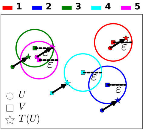
Figure 4: $\varepsilon$-congruence with respect to $L_{2}$. $U$ is marked with circles, $V$ with squares, and the translated configuration $T\left(U\right)$ with stars. Each of the $m=5$ robots is denoted by a different color. If each star falls inside its corresponding ball then the balls’ (common) radius corresponds to a valid translation. The $\varepsilon$-congruence is the minimal valid radius.

We denote $\varepsilon$-congruence with respect to $L_{2}$ and $L_{\infty}$ by $\varepsilon_{2}$ and $\varepsilon_{\infty}$, respectively. See an illustration in Figure 4.

Note that $\varepsilon$-congruence satisfies all the properties of a pseudosemimetric, and in case $L$ satisfies the triangle inequality (which is the case for $L_{2}$ and $L_{\infty}$) then $\varepsilon$-congruence is a pseudometric and therefore can be used with any nearest-neighbor data structure.

Shape-based metric. To measure the mismatch between two point sets, Kendall introduced the notion of a shape space (Kendall, 1984). Specifically, given $m$ $k$-dimensional points the shape space $\Sigma_{k}^{m}=\mathbb{R}^{k\times m}/\mathcal{S}$ is the quotient space of $\mathbb{R}^{k\times m}$ by the group of similarities generated by translations, rotations and dilations. Namely, it is a subdivision of all point sets into equivalence classes, where two point sets are equivalent if one can be transformed to the other by some operation $T\in\mathcal{S}$.

Let $U=\left(u_{1},\ldots,u_{m}\right),V=\left(v_{1},\ldots,v_{m}\right)\in\Sigma_{k}^{m}$ and $T\in\mathcal{S}$. Note that by the definition of equivalence sets we have that the distance between $U$ and $V$ is equal to the distance between $T(U)$ and $V$. This allows us to define the mismatch between $U$ and $V$ as the minimal distance over all similarities $T\in\mathcal{S}$. Specifically, Kendall uses the sum of squares of distances between associated pairs of points. Thus, the distance between two point sets is defined as

$$\min_{T\in\mathcal{S}}\left\{\sum_{i=1}^{m}\left(L_{2}\left(\left[T\left(U\right)\right]_{i},v_{i}\right)\right)^{2}\right\}.$$ (1)

We propose to adapt these ideas to the setting of MRMP. Specifically, in our basic setting we have that (i) each single-robot configuration is a planar point in $\mathbb{R}^{2}$ (ii) we restrict the set of similarities $\mathcal{S}$ to translations only. Thus, we can rewrite Equation 1 as:

$$\min_{T\in\mathbb{R}^{2m}}\left\{\sum_{i=1}^{m}\left(L_{2}\left(T_{i},v_{i}-u_{i}\right)\right)^{2}\right\},$$ (2)

where $T_{i}$ is the translation component in $T$ of the $i$-th point.

We restrict $\mathcal{S}$ to translations only since we are using a local planner that generates a straight-line path for each robot. Such local planning between a configuration $U$ and a translation of it $T\left(U\right)$ is always free of robot-robot collisions. However, it may not be free of collisions if we allow rotations and dilations.

The translation $T$ that minimizes Equation 2 is known as the centroid of the set $\left\{v_{i}-u_{i}\right\}_{i=1}^{m}$ (see (Protter and Morrey, 1970, pp. 520)). For two-dimensional points ($k=2$) the minimal value is

$$\textup{Ctd}\left(U,V\right)\!=\!\sum_{i=1}^{m}{\left(x_{i}^{2}+y_{i}^{2}\right)}-\frac{\left(\sum_{i=1}^{m}x_{i}\right)^{2}+\left(\sum_{i=1}^{m}y_{i}\right)^{2}}{m},$$ (3)

where $x_{i}$ and $y_{i}$ are the $x$ and $y$ coordinates of $v_{i}-u_{i}$. Equation 3 defines the Centroid distance in 2D, which we denote by Ctd.

In summary, we have presented five metrics for MRMP: the more traditional $\Sigma L_{2}$ and $\max L_{2}$, and the novel metrics $\varepsilon_{2}$, $\varepsilon_{\infty}$, Ctd. We will evaluate these five metrics below.

5 Canonical Substructures in $\mathcal{C}$-space

Here we introduce a new approach to better conquer the intricate problem of MRMP. We identify several “gadgets”, which represent local instances of the problem, and which force the robots to coordinate in a specific and prescribed manner. Those gadgets can be viewed as a set of representative tasks that need to be carried out in typical scenarios of MRMP. Examining these substructures, rather than the entire complex problem, has two benefits. Firstly, such substructures can be straightforwardly decomposed into a small number of equivalence classes (ECs) of (joint) configurations, which can be viewed as a discrete summary of the continuous problem. We conjecture that a metric which maximizes the number of explored ECs by a given planner also leads to better performance of the planner. Secondly, those ECs of a given substructure, and the relations between them, induce a natural distance metric, which faithfully quantifies how difficult it is to move between any given pair of joint configurations. This gives an additional method to assess the quality of a given metric by comparing it to the natural metric.

In the remainder of this section we describe three such canonical substructures, which we refer to as Permutations, Partitions, and Pebbles, and denote them by $\mathbb{X}_{\textup{Permutations}},\mathbb{X}_{\textup{Partitions}},\mathbb{X}_{\textup{Pebbles}}$. We also describe their corresponding natural metrics. In Section 6 we describe tools for analysis of metrics. Of course there could be many more useful substructures—see comment in the concluding section.

Each such substructure $\mathbb{X}$ is a subset of the joint $\mathcal{C}$-space $\mathcal{X}^{m}$. For every $\mathbb{X}$ we identify a finite collection of $e>0$ disjoint subsets $X_{1},\ldots,X_{e}$ of $\mathbb{X}$ termed equivalence classes (ECs). Note that each EC is a subset of the joint $\mathcal{C}$-space. We say that two joint configurations $U,V\in\mathbb{X}$ are equivalent if they belong to the same EC $X_{i}$. If robots can also leave one EC $X_{i}$ and enter another $X_{i^{\prime}}$, without going through any other EC then we say that the ECs $X_{i},X_{i^{\prime}}$ are neighbors. This gives rise to the equivalence graph $G_{\mathbb{X}}$ whose vertices are the ECs of $\mathbb{X}$, and there is an edge between every two neighboring ECs.

We are now ready to define the natural distance $\mathrm{d}_{\mathcal{K}}$ between two given joint configurations $U,V\in\mathbb{X}$. For a given $U\in\mathbb{X}$ denote by $\mathrm{EC}\left(U\right)$ the EC of $\mathbb{X}$ in which it resides. Then the natural distance $\mathrm{d}_{\mathcal{K}}\left(U,V\right)$ is the graph distance over $G_{\mathbb{X}}$ between $\mathrm{EC}(U)$ and $\mathrm{EC}(V)$, namely the number of edges along the shortest path in the graph between the vertices corresponding to $\mathrm{EC}(U),\mathrm{EC}(V)$.

5.1 Permutations

As an example of $\mathbb{X}_{\textup{Permutations}}$ consider the “Tunnel” scenario depicted in Figure 5. The workspace consists of three portions corresponding to the three “arms” of the workspace: upper arm, right arm and left arm, denoted by $\mathcal{A}=\left\{A_{U},A_{R},A_{L}\right\}$. In this substructure we define the ECs to correspond to the assignment of robots to portions of the tunnel, and to the specific order of the robots within each portion. The order in the upper arm $A_{U}$ is calculated according to decreasing $y$ coordinate, in the right arm $A_{R}$ according to decreasing $x$ coordinate, and in the left arm $A_{L}$ according to increasing $x$ coordinate. See Figure 5b for an illustration.

Two ECs are neighbors if they correspond to a transition of a single robot that leaves one arm and enters another. For instance, $\left[\left(3,4,2\right),\left(5,6,1\right),\left(\;\right)\right]$ and $\left[\left(3,4,2,1\right),\left(5,6\right),\left(\;\right)\right]$ are neighbors. This condition implicitly induces the equivalence graph $G_{\mathbb{X}_{\textup{Permutations}}}$ and the corresponding natural metric $\mathrm{d}_{\mathcal{K}}$. For instance, for any two configurations $U,V$ which lie in the ECs $\left[\left(3,4,2,5,6,1\right),\left(\;\right),\left(\;\right)\right]$ , $\left[\left(3,4,1,6,5,2\right),\left(\;\right),\left(\;\right)\right]$ , respectively, it follows that $\mathrm{d}_{\mathcal{K}}(U,V)=10$.

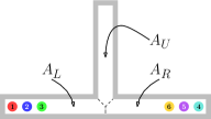
(a)

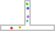
(b)

Figure 5: Tunnel scenario. The environment consists of a T-shaped free space and requires the robots in one side to exchange places with the robots on the other side. There are 6 translating disc robots of radius 2 and the width of each arm is 5, so the robots cannot exchange places within an arm without leaving it. (a) Start configuration. The red, blue and green robots lie on the left arm, and the yellow, purple and cyan robots lie on the right arm. In the goal configuration the red, blue and green robots lie on the right arm and the yellow, purple and cyan robots lie on the left arm. More specifically, the red robot exchanges places with the cyan robot, the blue robot with the purple robot and the green robot with the yellow robot. (b) A configuration for which the permutation in $A_{U}$ is $\left(3,2,5,4\right)$, in $A_{R}$ is $\left(\;\right)$ and in $A_{L}$ is $\left(1,6\right)$. The corresponding EC is denoted by $\left[\left(3,2,5,4\right),\left(\;\right),\left(1,6\right)\right]$.

An illustration for the equivalence graph for the case of $m=2$ robots is depicted in Figure 6.

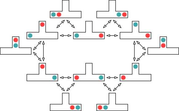
Figure 6: $G_{\mathbb{X}_{\textup{Permutations}}}$ for two robots ($m=2$). Each vertex of $G_{\mathbb{X}_{\textup{Permutations}}}$ represents an EC in the joint $\mathcal{C}$-space $\mathcal{X}^{m}$.

5.2 Partitions

As an example of $\mathbb{X}_{\textup{Partitions}}$ we consider the “Chambers” scenario depicted in Figure 7. Each EC is associated with a partitioning of the robots to the chambers. Each robot is mapped to the chamber that has the largest intersection with the robot and we choose a chamber at random in case that there is a tie. See Figure 7b. Two ECs are neighbors if exactly one robot changes its mapped chamber. Unlike the previous substructure, here the exact order of the robots inside one chamber does not matter.

5.3 Pebbles

The “8-Puzzle” scenario, which is a geometric variation of the classic 15-Puzzle (Archer, 1999), is used as an example for $\mathbb{X}_{\textup{Pebbles}}$. The problem is depicted in Figure 8. Unlike the discrete version of the puzzle, where each robot can occupy only one of nine possible places, in the geometric generalization the robots can lie in any collision-free configuration.

Each EC of $\mathbb{X}_{\textup{Pebbles}}$ is associated with an assignment of robots to the nine cells. The cell corresponding to each robot is the one that has the largest intersection with the robot, with the restriction that at most one robot is assigned to a single cell, and we choose a cell at random in case that there is a tie. An example for a configuration along with its correspondent assignment is described in Figure 8b. Two ECs of $\mathbb{X}_{\textup{Pebbles}}$ are neighbors if exactly one robot changes its cell assignment.

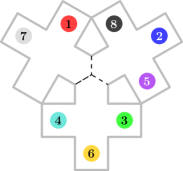
(a)

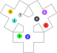
(b)

Figure 7: Chambers scenario. The environment consists of three chambers. The structure of each chamber allows the robots to exit from the chamber in any order, not necessarily in the order they entered to the chamber (as opposed to the arms in the Tunnel scenario). (a) Start configuration. (b) A configuration that corresponds to the assignment $\left[\left\{1,5,8\right\},\left\{4,6,7\right\},\left\{2,3\right\}\right]$. The natural distance between it and the configuration in Figure 7a is 4.

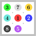
(a)

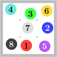
(b)

Figure 8: 8-Puzzle scenario. The environment can be naturally partitioned into nine cells that form a 3$\times$3 grid. A robot can translate only between adjacent cells. (a) Start configuration. The goal is to arrange the robots in the order $r_{1},\ldots,r_{m}$, i.e., $r_{1}$ is situated in the cell in the top left corner, and so on. (b) A configuration that corresponds to the assignment $\left[\left\{4\right\},\left\{3\right\},\left\{6\right\},\left\{\;\right\},\left\{7\right\},\left\{2\right\},\left\{8\right\},\left\{1\right\},\left\{5\right\}\right]$. The natural distance between it and the configuration in Figure 8a is 5 since there is a discrete motion mimicking five transfer steps each of a single pebble from one cell to another in an 8-puzzle, that transforms one configuration to the other (the motion involves the purple, red, grey, green and cyan robots).

6 Analysis of Metrics

In this section we introduce two novel tools for analyzing metrics, which rely on the concept of canonical substructures, described in Section 5. The following tools assess the quality of a given metric $\mathrm{d}$ by quantifying its similarity to the natural metric $\mathrm{d}_{\mathcal{K}}$, and by counting the number of explored ECs by a planner that is paired with $\mathrm{d}$.

In addition to the tools described in this section, we have a visualization tool that automatically generates an animation for the expanded tree produced by the RRT-style planner. Some properties of the metrics can be inferred by perusing the animations. This tool was essential in the screening phase and guiding our choice of metrics. Links to example videos can be found in Appendix B.

6.1 Distributions separation

The following technique requires as an input, after fixing a specific canonical substructure $\mathbb{X}$, a set of $\ell$ randomly sampled joint configurations $\mathbb{C}=\{C_{1},\ldots,C_{\ell}\}$ from $\mathbb{X}$. Each such sample is then classified according to its EC in $\mathbb{X}$.

Our working hypothesis is that a good metric should faithfully reflect the natural distance, and in the rest of the subsection we spell out what it means to have this property.

When incorporating the metric into a sampling-based planner, the role of the metric is to compare distances between different pairs of sampled configurations. Given two pairs of configurations $\left(U_{1},V_{1}\right)$ and $\left(U_{2},V_{2}\right)$, the planner favors to check the continuous motion between the first pair in case the distance between $U_{1},V_{1}$ is smaller than the distance between $U_{2},V_{2}$ (Note that in the case of an RRT-style planner, the compared pairs always satisfy $U_{1}=U_{2}$.). How much a metric reflects the natural distance can be measured by how well the relation between distances of different pairs of configurations is preserved when compared to the natural distance. Preserving the natural distance can be measured by $\Gamma_{\mathrm{d}}$:

$$\Gamma_{\mathrm{d}}\!=\underset{U_{1},U_{2},V_{1},V_{2}\in\mathbb{X}}{\Pr}\Bigl{[} \mathrm{d}\!\left(U_{1},V_{1}\right)<\mathrm{d}\!\left(U_{2},V_{2}\right)\Bigm{|}\;\Bigr{.}$$

. $$\mathrm{d}_{\mathcal{K}}\left(U_{1},V_{1}\right)<\mathrm{d}_{\mathcal{K}}\left(U_{2},V_{2}\right)\Bigr{]}.$$

In one extreme case, if we use the natural distance as $\mathrm{d}$ we have $\Gamma_{\mathrm{d}}=1$. In the other extreme case, if a metric $\mathrm{d}$ has no correlation with the natural distance we have $\Gamma_{\mathrm{d}}=0.5$. We are interested in a metric that gives a large value of $\Gamma_{\mathrm{d}}$.

In the rest of the subsection we formalize the discussion above and explain how to calculate and compare $\Gamma_{\mathrm{d}}$ between different metrics. For every possible (discrete) value of the natural distance $\alpha\in\operatorname{Im}\mathrm{d}_{\mathcal{K}}$ we compute the set ${\mathcal{D}_{\mathrm{d}}\!}^{\alpha}$ of metric distances given that the natural distance is $\alpha$:

$${\mathcal{D}_{\mathrm{d}}\!}^{\alpha}=\left\{\mathrm{d}\!\left(U,V\right)\mid U,V\in\mathbb{C},\mathrm{d}_{\mathcal{K}}\left(U,V\right)=\alpha\right\}.$$

With a slight abuse of notation, we treat ${\mathcal{D}_{\mathrm{d}}\!}^{\alpha}$ as a distribution over pairs of configurations from $\mathbb{X}$. Here we use the fact that $\mathbb{C}$ captures the structure of $\mathbb{X}$. Furthermore, we define $\mathcal{D}_{\mathrm{d}}\!=\left\{{\mathcal{D}_{\mathrm{d}}\!}^{\alpha}\mid\alpha\in\operatorname{Im}\mathrm{d}_{\mathcal{K}}\right\}$. Consequently, $\Gamma_{\mathrm{d}}$ can be represented as

$$\Gamma_{\mathrm{d}}=\Pr\Bigl{[}\alpha_{0}<\beta_{0}\;\Bigm{|}\;\alpha_{0}\sim{\mathcal{D}_{\mathrm{d}}\!}^{\alpha},\beta_{0}\sim{\mathcal{D}_{\mathrm{d}}\!}^{\beta},\alpha<\beta\Bigr{]},$$

where the notation $\alpha_{0}\sim{\mathcal{D}_{\mathrm{d}}\!}^{\alpha}$ indicates that $\alpha_{0}$ is sampled from the distribution ${\mathcal{D}_{\mathrm{d}}\!}^{\alpha}$.

Sampling-based planners usually attempt to connect nearby configurations. Thus, it is more important to identify close configurations than remote ones. Pairs of far-away configurations (with respect to the natural distance) are practically ignored by a sampling-based planner that uses a reasonable metric $\mathrm{d}$. We restrict $\Gamma_{\mathrm{d}}$ to natural distances of at most a threshold parameter $\tau$, using the following definition of ${\Gamma_{\mathrm{d}}\!}^{\tau}$:

$${\Gamma_{\mathrm{d}}\!}^{\tau}=\Pr\Bigl{[}\alpha_{0}<\beta_{0}\;\Bigm{|}\;\alpha_{0}\sim{\mathcal{D}_{\mathrm{d}}\!}^{\alpha},\beta_{0}\sim{\mathcal{D}_{\mathrm{d}}\!}^{\beta},\alpha<\beta,\alpha\leq\tau\Bigr{]}.$$

We expect that a metric $\mathrm{d}_{1}$ will be more effective than a metric $\mathrm{d}_{2}$ if ${\Gamma_{\mathrm{d}_{1}\!}}^{\tau}>{\Gamma_{\mathrm{d}_{2}\!}}^{\tau}$.

Note that the value of $\tau$ depends on the specific setting. Here we present general guidelines for choosing $\tau$. An exact method is left for future work. Recall that in each iteration of an RRT-style planner a configuration $V$ is sampled at random, and its nearest-neighbor $U$ (from the currently growing tree) is picked. A proper value for $\tau$ satisfies $\mathrm{d}_{\mathcal{K}}\left(U,V\right)\leq\tau$ with high probability for a typical RRT-tree size. Pairs of configurations for which the natural distance is larger than $\tau$ are practically ignored by a sampling-based planner, and should not be taken into account in the calculation of $\Gamma_{\mathrm{d}}$.

6.2 Explored equivalence classes

RRT-style planners, as the one used and described later on in Section 7, explore the $\mathcal{C}$-space from a starting configuration. A desirable property of such planners is to reach various regions of interest in the $\mathcal{C}$-space. In our setting, we measure the quality of exploration by the number of different ECs reached, where a larger number of explored ECs means that the planner explores the $\mathcal{C}$-space more exhaustively. Since the planner cannot foresee which parts of the $\mathcal{C}$-space can lead to a solution, we expect that an effective metric will result in a larger number of explored ECs when compared to an ineffective one.

We propose the following experiment to assess $\mathrm{d}$ with respect to the quality of exploration. A single-tree RRT-style planner is used to build a tree with $N$ vertices. The set of explored configurations is denoted by $\mathcal{U}_{\mathrm{d}}$. For each configuration $U\in\mathcal{U}_{\mathrm{d}}$ we identify its representative EC denoted by $\mathrm{EC}\left(U\right)$. We count the number of distinct explored ECs, i.e., the number of distinct ECs in the set $\left\{\mathrm{EC}\left(U\right)\;|\;U\in\mathcal{U}_{\mathrm{d}}\right\}$, and denote it by $\left|\mathcal{U}_{\mathrm{d}}/\mathrm{EC}\right|$. We anticipate that a metric $\mathrm{d}_{1}$ will be more effective than a metric $\mathrm{d}_{2}$ if $\left|\mathcal{U}_{\mathrm{d}_{1}}/\mathrm{EC}\right|>\left|\mathcal{U}_{\mathrm{d}_{2}}/\mathrm{EC}\right|$.

7 Experimental Results

In this section we make use of the tools developed in Section 6 to analyze the properties of the metrics in the scenarios described in Section 5. Then we compare the effectiveness of the metrics as used by dRRT (Solovey et al., 2016) to solve instances of MRMP. As mentioned in Section 3, dRRT is an extension of RRT, which allows it to cope with a greater number of robots and more complex scenarios. Later on we show the effectiveness of the planner incorporated with different metrics in a general environment that consists of several substructures.

On the implementation side, our testing environment is implemented in C++ and relies on Open Motion Planning Library (OMPL) (Sucan et al., 2012). While we are not concerned with running times in this work, we mention that all the metrics defined in Section 4 can be implemented with running time linear in the number of robots. Refer to Appendix A for full description of the implementation.

7.1 Analyzing properties of the metrics

We show and analyze the results of the experiments described in Section 6 using the scenarios described in Section 5.

For each scenario, we show results for the value of ${\Gamma_{\mathrm{d}}\!}^{\tau}$ defined in Section 6.1. Then, we count the number of distinct explored ECs, as suggested in Section 6.2. In order to do so, we use a dRRT-tree with 10,000 vertices rooted at the start configuration (see Figures 5a, 8a and 7a) . Finally, we show the effectiveness of an entire planning algorithm that uses each of the metrics and show how it correlates with the results of the analysis tools. We measure the effectiveness of the planner by inspecting both  (i) the number of explored vertices when a solution is found—the lower the number, the more effective we consider the metric to be; (ii) the success rate of the planner. We mention that the success rate of the local planner (and not the motion planner) is similar among all the metrics, and therefore we do not report it. We do not measure running times since we are interested only in the analytic effectiveness of each metric.

Next, for each typical scenario we describe (i) the results of the distributions-separation predicates, (ii) the results of the ECs exploration, and finally (iii) the actual behavior of the planner and its relation to the predictions. These are also summarized in Table 1, Figure 10 and Figure 11, respectively.

Permutations substructure. Figure 9 shows subsets of the sets of distributions $\mathcal{D}_{\varepsilon_{2}}$ and $\mathcal{D}_{\Sigma L_{2}}$ for the Tunnel scenario: observe that the distributions in $\mathcal{D}_{\varepsilon_{2}}$ are better separated than the distributions in $\mathcal{D}_{\Sigma L_{2}}$. This separation is expressed by the dissimilarities between the different distributions. For example, the common area bounded by the blue and green distributions (representing ${\mathcal{D}_{\mathrm{d}}\!}^{0}$ and ${\mathcal{D}_{\mathrm{d}}\!}^{4}$ respectively) is smaller for $\varepsilon_{2}$ when compared to $\Sigma L_{2}$. This is also the case for the green and red distributions (representing ${\mathcal{D}_{\mathrm{d}}\!}^{4}$ and ${\mathcal{D}_{\mathrm{d}}\!}^{6}$ respectively). The value ${\Gamma_{\mathrm{d}}\!}^{\tau}$ quantifies the distribution separation. For this scenario we set $\tau=4$. The values of ${\Gamma_{\mathrm{d}}\!}^{\tau}$ are given in Table 1. The values for $\varepsilon_{2}$, $\varepsilon_{\infty}$ and Ctd are similar to each other, and are larger than the values for $\Sigma L_{2}$ and $\max L_{2}$.

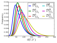
(a) $\mathcal{D}_{\Sigma L_{2}}$

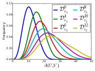
(b) $\mathcal{D}_{\varepsilon_{2}}$

Figure 9: Distributions from $\mathcal{D}_{\mathrm{d}}$ for $\Sigma L_{2}$ and $\varepsilon_{2}$ metrics in the Tunnel scenario. Better reflection of the natural distance is expressed by higher level of separability between the distributions.

Scenario	$\boldsymbol{\tau}$	Metric ($\boldsymbol{\mathrm{d}}$)
		$\Sigma L_{2}$	$\max L_{2}$	$\varepsilon_{2}$	$\varepsilon_{\infty}$	Ctd
Tunnel	4	0.810	0.843	0.904	0.904	0.907
Chambers	1	0.858	0.983	0.971	0.962	0.938
8-Puzzle	7	0.953	0.938	0.951	0.921	0.971

Table 1: The value of ${\Gamma_{\mathrm{d}}\!}^{\tau}$ for different metrics in different scenarios. Each entry in the table is the value of ${\Gamma_{\mathrm{d}}\!}^{\tau}$ for the corresponding $\mathrm{d}$, $\tau$ and scenario. Larger values mean higher distributions separation, and in turn better effectiveness is expected. The value of $\tau$ is set according to the guidelines described in Section 6.1

.

The number of distinct explored ECs is shown in Figure 10a: observe that Ctd and $\varepsilon$-congruence-type metrics show better results when compared to the standard metrics. In addition, we expect that $\varepsilon_{2}$ and Ctd will be more effective than $\varepsilon_{\infty}$. Furthermore, $\Sigma L_{2}$ shows better results than $\max L_{2}$.

As described in Figure 11a, the effectiveness of the metrics correlates with the analysis of Section 6. As expected, $\varepsilon_{2}$, $\varepsilon_{\infty}$ and Ctd are more effective than $\Sigma L_{2}$ and $\max L_{2}$.

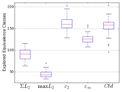
(a) Permutations Substructure

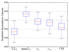
(b) Partitions Substructure

(c) Pebbles Substructure

Figure 10: Different explored equivalence classes experiment. A dRRT tree is expanded until it contains 10,000 vertices. For each vertex in the tree we find its representative EC, and count the number of different ECs (denoted by $\left|\mathcal{U}_{\mathrm{d}}/\mathrm{EC}\right|$). Higher value means that we expect the metric to be more effective. The experiment is repeated 50 times for each metric. The figure depicts the values of $\left|\mathcal{U}_{\mathrm{d}}/\mathrm{EC}\right|$ for each metric.

(a) Permutations Substructure

(b) Partitions Substructure

(c) Pebbles Substructure

Figure 11: Number of expanded vertices when a solution is found. The experiment is repeated 50 times per metric. The planner success rate is depicted in the green labels on top of each boxplot. The red labels are the median value. Effectiveness is expressed by high success rate and low number of vertices.

Partitions substructure. For the distributions separation we use $\tau=1$. The values of ${\Gamma_{\mathrm{d}}\!}^{\tau}$ are given in Table 1. $\max L_{2}$ has the largest value, then come $\varepsilon_{2}$, $\varepsilon_{\infty}$ and Ctd, while $\Sigma L_{2}$ is far behind.

Figure 10b shows the number of distinct explored ECs. $\max L_{2}$ shows the best results, $\varepsilon_{2}$ and $\varepsilon_{\infty}$ have comparable results, which are better than Ctd, and $\Sigma L_{2}$ yields the poorest results.

For this scenario, by looking at the results of the experiments described in Section 6, one can foresee that $\max L_{2}$, $\varepsilon_{\infty}$ and $\varepsilon_{2}$ will be more effective than Ctd, which in turn, will be more effective than $\Sigma L_{2}$. This is indeed the case when measuring the effectiveness of the planner, as can be seen in Figure 11b.

Pebbles substructure. For the calculation of ${\Gamma_{\mathrm{d}}\!}^{\tau}$ we use $\tau=7$. The values are given in Table 1. The best value is achieved by Ctd, then $\varepsilon_{2}$ and $\Sigma L_{2}$ have comparable values, then comes $\max L_{2}$ and finally $\varepsilon_{\infty}$ with the smallest value.

The number of distinct explored ECs is shown in Figure 10c. Here again, the largest number of explored ECs is achieved with Ctd, followed by $\varepsilon_{2}$ and $\Sigma L_{2}$. Then $\varepsilon_{\infty}$, and the lowest value is for $\max L_{2}$.

The effectiveness of the planner incorporated with each metric is expressed in Figure 11c. The results are with accordance to the analysis: Ctd is the most effective metric, $\Sigma L_{2}$ and $\varepsilon_{2}$ have comparable effectiveness, and $\varepsilon_{\infty}$ and $\max L_{2}$ are the less effective metrics.

7.2 Putting it all together

The $\mathcal{C}$-space of a general MRMP problem may consist of several substructures. This is the case for the scenario depicted in Figure 12a, which contains $m=8$ robots. Figure 12c shows the effectiveness of planning with each metric. As can be inferred from the results, even in more general scenarios, the novel metrics are more effective than the standard ones. In some cases, it may be beneficial to alternate between several metrics—the planner maintains several nearest-neighbors data-structures, each for a different metric. Each time the tree is expanded, a different data-structure is used in a round-robin fashion.

We have tested the scenario depicted in Figure 12a with 4, 6 and 8 robots (for 4 and 6 robots we eliminate from the scenario the robots $r_{5},\ldots,r_{8}$ and $r_{7},r_{8}$ respectively). We used each of the five metrics, along with all the combinations of two out of the five (total of $15$) metrics. For the scenario with $m=4$ robots, the effectiveness of all the metrics and their alternation was comparable. The results for the scenario with $m=6$ robots (see Figure 12b) support the claim that it may be better to alternate between different metrics. Note the interesting fact that when alternating between $\varepsilon_{2}$ and $\Sigma L_{2}$ or Ctd, better effectiveness is obtained than when using each metric separately. For the scenario with $m=8$ robots (Figure 12c) the novel metrics are more effective when compared to the standard ones. Alternating between novel and standard metrics does not make the planner more effective for the case of $8$ robots. As we move from $4$ robots (easier) to $8$ robots (considerably harder), the effectiveness of the metrics becomes more noticeable.

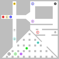
(a)

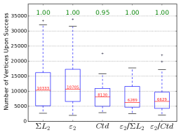
(b) Effectiveness with 6 robots

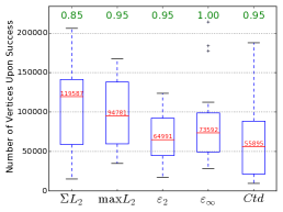
(c) Effectiveness with 8 robots

Figure 12: A general scenario. We test the scenario with 8 robots, and the scenario with 4 or 6 robots which we get by eliminating $r_{5},\ldots,r_{8}$ or $r_{7},r_{8}$, respectively. (a) Start and goal configuration, drawn in solid and empty discs, respectively. (b) Effectiveness of metrics and alternation between metrics summarized over 20 runs for the case of $6$ robots. As in the previous plots, the green labels indicate the success rate. (c) Effectiveness of each metric summarized over 20 runs of the planner for the case of $8$ robots.

8 Other Multi-Robot Systems

In this section we show how to extend the metrics that were defined in Section 4 to cope with rotating robots in 2D. We also show experimental results that demonstrate the suitability of the novel metrics for rotating robots.

We mention that all metrics can be extended to 3D settings (with rigid-body motions) straightforwardly. Extensions for other robotics systems, e.g., robots with dynamic constraints, is beyond the scope of this paper and is left for future work.

8.1 Metrics definition

Let $U=\left(u_{1},\ldots,u_{m}\right),V=\left(v_{1},\ldots,v_{m}\right)\in\mathcal{X}^{m}$ be two multi-robot configurations. Each single-robot configuration $w\in\mathcal{X}$ can be represented as three coordinates $x\left(w\right),y\left(w\right),\theta\left(w\right)$ for which $x\left(w\right),y\left(w\right)\in\mathbb{R}$ and $\theta\left(w\right)\in\left[-\pi,\pi\right)$. Define:

$$x_{i}=x\left(v_{i}\right)-x\left(u_{i}\right),$$

$$y_{i}=y\left(v_{i}\right)-y\left(u_{i}\right),$$

$$\theta_{i}=\begin{cases}\left|\theta\left(v_{i}\right)-\theta\left(u_{i}\right)\right|,&\left|\theta\left(v_{i}\right)-\theta\left(u_{i}\right)\right|<\pi\\ 2\pi-\left|\theta\left(v_{i}\right)-\theta\left(u_{i}\right)\right|,&\textup{otherwise}\end{cases}.$$

In addition, we introduce a weight parameter $0\leq s\leq 1$ which determines the weight between the translation and the rotation components.

Having defined $x_{i},y_{i},\theta_{i}$, the traditional metrics $\Sigma L_{2}$ and $\max L_{2}$ can be trivially extended:

$$\Sigma L_{2}\left(U,V\right) =\sum_{i=1}^{m}\left(s\sqrt{x_{i}^{2}-y_{i}^{2}}+\left(1-s\right)\theta_{i}\right),$$

$$\max L_{2}\left(U,V\right) =\max_{i=1,\ldots,m}\left(s\sqrt{x_{i}^{2}-y_{i}^{2}}+\left(1-s\right)\theta_{i}\right).$$

Similarly, we redefine $\varepsilon$-congruence and Ctd by treating the rotational component as an additional (scaled) coordinate in Euclidean space:

$$\varepsilon_{2}\left(U,V\right)=\mathrm{MiniBall}\left(\left\{\left(sx_{i},sy_{i},\left(1-s\right)\theta_{i}\right)\right\}_{i=1}^{m}\right),$$

$$\varepsilon_{\infty}\left(U,V\right)=\mathrm{MiniCube}\left(\left\{\left(sx_{i},sy_{i},\left(1-s\right)\theta_{i}\right)\right\}_{i=1}^{m}\right).$$

Ctd $$\left(U,V\right)\!=\!$$

$$\sum_{i=1}^{m}{\left(\left(sx_{i}\right)^{2}+\left(sy_{i}\right)^{2}+\left(\left(1-s\right)\theta_{i}\right)^{2}\right)}-$$

$$\frac{\left(\sum_{i=1}^{m}sx_{i}\right)^{2}+\left(\sum_{i=1}^{m}sy_{i}\right)^{2}+\left(\sum_{i=1}^{m}\left(1-s\right)\theta_{i}\right)^{2}}{m}.$$

Note that for the case of $s=1$ (translation only) the metrics are identical to those discussed in Section 4.

8.2 Experimental results

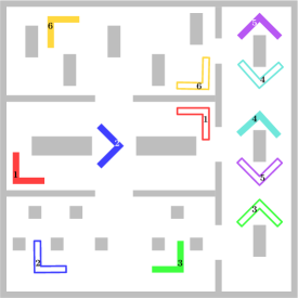
(a) Scenario

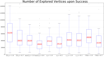
(b) Effectiveness of metrics

Figure 13: A scenario with $m=6$ rotating robots in the plane. The robots are L-shaped and must rotate to arrive from the start configurations to the goal configurations. (a) Start and goal configurations are drawn in solid and empty L-shaped, respectively. (b) Number of expanded vertices when a solution is found. The red labels are the median value. The experiment is repeated 50 times per metric and weight parameter $s$. Effectiveness is expressed by low number of expanded vertices.

We use the scenario depicted in Figure 13a. The robots in that scenario are L-shaped and allowed to rotate.

One difficulty that arises is deciding a proper value for the weight parameter $s$. Previous research has already addressed this problem (Amato et al., 2000; Kuffner, 2004). In our experiments we empirically chose the optimal value; we repeated the experiments 50 times for each value $s=0.1,0.2,\ldots,0.9$ and picked the one that leads to the most effective planning. Note that the optimal value may be different for different metrics.

Figure 13b shows the effectiveness of planning with each metric when the rotation component is taken into account. For each metric we show the effectiveness for $s=1$ and for the optimal value of $s$. It can be seen from the figure that the adaptation of the metrics for rotating robots takes rotation into account in a reasonable way; the effectiveness improves when we weigh in the rotation component of the robots. An exception is the case of $\varepsilon_{\infty}$, in which the improvement we get with the optimal value of $s$ (when compared to $s=1$) is not significant.

According to Figure 13b, the most effective metrics are $\max L_{2}$ and $\varepsilon_{2}$. Then, Ctd, and finally, the least effective metrics are $\varepsilon_{\infty}$ and $\Sigma L_{2}$.

9 Conclusions and Future Work

Our work suggests that in order to effectively solve MRMP using sampling-based planners one should employ tailored multi-robot metrics, possibly side-by-side with more traditional metrics.

An immediate question is how to efficiently combine the benefits of different metrics. This resembles the idea of combining different heuristics in search-based algorithms (Aine et al., 2016). We propose to borrow ideas from this domain to address our problem. One approach may be to grow several trees, one for each metric. The trees can share states (such as SMHA* (Aine et al., 2016)) and choosing which tree to grow at each point can be done in a dynamic fashion (see, e.g., (Phillips et al., 2015)).

This work has utilized three substructures and their combination in order to asses metrics. Of course there could be many more substructures, in particular larger, more elaborate ones, which would possibly improve our understanding of metrics. Thus, it would certainly be useful to automatically identifying these, possibly through a learning phase.

Metrics are relevant for other settings of MRMP, including those involving moving rigid bodies in 3D, and robots with differential constraints. The proposed metrics and analysis tools can be extended to such settings as well.

Another notable variant is the unlabeled setting in which all the robots are identical and interchangeable. There are similarity measures for unlabeled point sets that can be adapted for MRMP (Alt et al., 1988; Belongie et al., 2002; Efrat and Itai, 1996; Hausdorff, 1927; Huttenlocher et al., 1993). Unlabeled planning involves matching functions as well, which have common properties with metrics but make the problem considerably harder. We have began to explore the unlabeled case, and have some promising initial results in this direction as well. A demonstration of our initial results for unlabeled disc robots is provided in Appendix C.

In this work we assessed metrics using RRT-style planners, and specifically dRRT (see Section 3). Although we do not believe that our reported results are biased towards these specific types of planners, it would be interesting to see whether the conclusions can be reproduced for other planners, that operate differently than RRT, e.g., PRM*, RRT* (Karaman and Frazzoli, 2011) and FMT* (Janson et al., 2015). This also leads to the question of the effect metrics have on the quality of the solution paths in MRMP.

Funding

This work has been supported in part by the Israel Science Foundation (grant no. 825/15), by the Blavatnik Computer Science Research Fund, and by the Blavatnik Interdisciplinary Cyber Research Center at Tel Aviv University. Kiril Solovey is supported by the Clore Israel Foundation.

Appendix A Metrics Calculation

We consider the running time required for the calculation of each of the five metrics described in the paper. The calculation of $\Sigma L_{2}$, $\max L_{2}$ and Ctd is straightforward and requires $O\left(m\right)$ time, where $m$ is the number of robots. However, the implementation of $\varepsilon$-congruence-type metrics is a little more intricate.

Given the joint configurations $U,V$, $\varepsilon_{\infty}\left(U,V\right)$ can be calculated by first finding a smallest enclosing square of the set of $m$ points $\left\{v_{i}-u_{i}\right\}_{i=1}^{m}$ (denoted by $\mathrm{MiniCube}\left(\left\{v_{i}-u_{i}\right\}_{i=1}^{m}\right)$). Half of the square edge length is the value of $\varepsilon_{\infty}$. This yields a running time of $O\left(m\right)$, using only subtractions and comparisons.

$\varepsilon_{2}\left(U,V\right)$ can be calculated similarly, using the smallest enclosing disc of the set $\left\{v_{i}-u_{i}\right\}_{i=1}^{m}$ (denoted by $\mathrm{MiniBall}\left(\left\{v_{i}-u_{i}\right\}_{i=1}^{m}\right)$). The radius of the disc is the value of $\varepsilon_{2}$. The enclosing disc can be calculated in time $O\left(m\right)$ (Gärtner, 1999; Megiddo, 1983).

We now proceed to prove the correctness of the calculation for $\varepsilon_{2}$. The proof of correctness for $\varepsilon_{\infty}$ is analogous. Recall that we are given two sets of $m$ planar points $U=\left(u_{1},\ldots,u_{m}\right),V=\left(v_{1},\ldots,v_{m}\right)$, and our goal is to find the minimal value $R\in\mathbb{R}^{+}$ such that there exists a transformation $T:\mathbb{R}^{2}\rightarrow\mathbb{R}^{2}$ that satisfies

$$\max_{i=1,\ldots,m}L_{2}\left(T\left(u_{i}\right),v_{i}\right)\leq R.$$

We denote the minimal $R$ by $R^{*}$. For each $i=1,\ldots,m$ we define $\delta_{i}=v_{i}-u_{i}$ and let $\Delta=\left\{\delta_{1},\ldots,\delta_{m}\right\}$.

Let $R\in\mathbb{R}^{+}$. We observe that $R\geq R^{*}$ if and only if there is a point $p\in\mathbb{R}^{2}$ that lies in the intersection of the $m$ discs with radius $R$ centered at $\delta_{i}$ for $1\leq i\leq m$. The point $p$ can be viewed as a translation $T$ for which $\max\limits_{i=1,\ldots,m}L_{2}\left(T\left(u_{i}\right),v_{i}\right)\leq R$. Hence, the problem reduces to finding the minimal value of $R$ such that $m$ discs with radius $R$ centered at $\delta_{i}$ have a nonempty intersection. For a given $R$, the intersection is nonempty if and only if there is a point $q\in\mathbb{R}^{2}$ that satisfies

$$\max_{i=1,\ldots,m}L_{2}\left(q,\delta_{i}\right)\leq R.$$ (4)

On the one hand, if there exists a point $q\in\mathbb{R}^{2}$ that satisfies Equation 4, then the disc with radius $R$ centered at $q$ is an enclosing disc for $\Delta$. On the other hand, the center of any enclosing disc with radius $R$ of $\Delta$ satisfies Equation 4. In sum, for a given $R$, the intersection of the discs is nonempty if and only if there is an enclosing disc of $\Delta$ with radius $R$.

Hence, the radius of the minimal enclosing disc of $\Delta$ is the value of $\varepsilon_{2}\left(U,V\right)$.

Note that it can be easily extended to higher dimensions. In the above proof, one should replace $\mathbb{R}^{2}$ with $\mathbb{R}^{d}$ and “disc” with “ball”. It can also be extended to metrics other than $L_{2}$ (as is the case for $\varepsilon_{\infty}$).

The running times of $\Sigma L_{2}$, $\max L_{2}$, $\varepsilon_{\infty}$ and Ctd are almost identical. However, in practice the constant in the running time of $\varepsilon_{2}$ is non-negligible. Although there is a fundamental similarity between $\varepsilon_{2}$ and $\varepsilon_{\infty}$, when taking the running time into account, $\varepsilon_{\infty}$ has a slight advantage since it can be computed more quickly.

Appendix B Visualization Tool

In the initial phases of our study we used a visualization tool for illustrating the progress of the planner for different metrics, as more samples are added. The tool is based on Matplotlib (Hunter, 2007). It is used to generate videos that show the tree expansion process. Recall that each iteration of an RRT-style algorithm proceeds in the following fashion: (a) sampling a random configuration $V$ from the joint $\mathcal{C}$-space (b) finding its nearest neighbor $U$ in the tree (c) steering from $U$ in the direction of $V$, to obtain a configuration $W$ (d) calling the local planner to check the motion between $U$ and $W$ and adding $W$ to the tree in case the motion is free. The tool is used to visualize all these steps.

We provide videos that demonstrate the simulation of the process. See Figure 14 for a screenshot and basic explanation of the videos.

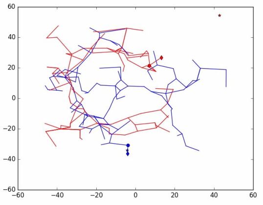
Figure 14: A screenshot of the visualization-tool output. Full-size videos are available at https://www.youtube.com/channel/UCVBp--RJj7l4q-sDBA_rTbg. Each robot is represented by a different color. In this scenario there are two robots ($m=2$), drawn in red and blue. The randomly-sampled configurations are drawn with stars. The chosen configurations from the tree (nearest neighbor of the random configuration) are drawn with circles. The configurations to steer to are drawn with diamonds. The drawn edges are the tree edges projected onto each robot configuration space. Sometimes it is more convenient to split the figure so that each robot has its own axis (refer to the youtube channel for such videos). In order to reduce video time we omitted iterations in which the planner fails to expand the tree.

As mentioned in the paper, one of the first type of metrics we have tested are metrics that have high correlation with the failure rate of the local planner. We denote such a metric by CPM (Closest Point Metric). The idea behind CPM is to calculate the closest point along the paths of any pair of robots, and accumulate all such closest points in order to predict how likely is the local planner to fail. We compared CPM against the traditional $\Sigma L_{2}$ in a scenario cluttered with random obstacles that involve two translating robots. The visualization that illustrates the tree growth process for each metric is available at https://www.youtube.com/playlist?list=PLQFVBs-JqK1JbaJbliRtN6Y4qCZm6fOSs. It is noticeable from the video that CPM causes the planner to explore configurations in which the robots are far away from each other, further causing them to be near the workspace boundary The analogues for the single-robot setting are configurations in which the robot is located far from the obstacles. Although it might be a desirable property for the single-robot setting, it raises difficulties for solving MRMP problems, since it is usually necessary to explore configurations in which the robots are not located near the workspace boundary.

Videos used for visualizing the planner for the Tunnel scenario are available at https://www.youtube.com/playlist?list=PLQFVBs-JqK1Jyv-6Kc1ofDVmFuHU48jlQ. The videos illustrate the growth process of the tree until it contains 500 vertices. One analysis tool that we describe in the paper is to count the number of distinct explored equivalence classes. We show in the paper that the novel metrics that we propose cause the planner to explore more equivalence classes when compared to the standard metrics. This phenomenon can be noticed in the videos. For example, let us focus only on the order of the robots that lie in the upper “arm” of the workspace. It can be observed that for $\Sigma L_{2}$ (https://youtu.be/8GBl6C9xxm8), in most of the configurations, the topmost robot is the yellow robot, then the green robot and after them is the blue robot. However, for $\varepsilon_{2}$ (https://youtu.be/M_3b7J6aabA), the order of the robots that lie in the upper arm is much more diverse. There are configurations in which the three topmost robots are the yellow, green and blue, while in other configurations the three topmost are the yellow, purple and cyan, and there are configurations in which the order begins with yellow, green and purple. When the number of vertices goes up, the phenomenon becomes more extreme, as we show in the paper.

Appendix C Extensions

As noted in the paper, our methods can be extended to other settings of MRMP. We already made some initial progress on settings in which the robots are interchangeable with each other, i.e., the so-called unlabeled case.

Animations of paths for the unlabeled setting are available at https://www.youtube.com/playlist?list=PLNHY_VaTYKopM2JDpVMrWoyIowB4gXe__. We note that the work on the unlabeled setting is preliminary.

References

- Adler et al. (2015) Adler A, de Berg M, Halperin D and Solovey K (2015) Efficient multi-robot motion planning for unlabeled discs in simple polygons. IEEE Trans. Automation Science and Engineering 12(4): 1309–1317.
- Aine et al. (2016) Aine S, Swaminathan S, Narayanan V, Hwang V and Likhachev M (2016) Multi-heuristic A*. I. J. Robotics Res. 35(1-3): 224–243.
- Alt et al. (1988) Alt H, Mehlhorn K, Wagener H and Welzl E (1988) Congruence, similarity, and symmetries of geometric objects. Discrete & Computational Geometry 3: 237–256.
- Amato et al. (2000) Amato NM, Bayazit OB, Dale LK, Jones C and Vallejo D (2000) Choosing good distance metrics and local planners for probabilistic roadmap methods. IEEE Trans. Robotics and Automation 16(4): 442–447.
- Archer (1999) Archer AF (1999) A modern treatment of the 15 puzzle. The American Mathematical Monthly 106(9): 793–799.
- Aronov et al. (1999) Aronov B, de Berg M, van der Stappen AF, Švestka P and Vleugels J (1999) Motion planning for multiple robots. Discrete & Computational Geometry 22(4): 505–525.
- Bareiss and van den Berg (2015) Bareiss D and van den Berg J (2015) Generalized reciprocal collision avoidance. I. J. Robotics Res. 34(12): 1501–1514.
- Belongie et al. (2002) Belongie SJ, Malik J and Puzicha J (2002) Shape matching and object recognition using shape contexts. IEEE Trans. Pattern Anal. Mach. Intell. 24(4): 509–522.
- Bharatheesha et al. (2014) Bharatheesha M, Caarls W, Wolfslag WJ and Wisse M (2014) Distance metric approximation for state-space RRTs using supervised learning. In: IEEE/RSJ International Conference on Intelligent Robots and Systems. pp. 252–257.
- Boeuf et al. (2015) Boeuf A, Cortés J, Alami R and Siméon T (2015) Enhancing sampling-based kinodynamic motion planning for quadrotors. In: IEEE/RSJ International Conference on Intelligent Robots and Systems. pp. 2447–2452.
- Bridgeman and Tamassia (2000) Bridgeman SS and Tamassia R (2000) Difference metrics for interactive orthogonal graph drawing algorithms. J. Graph Algorithms Appl. 4(3): 47–74.
- Brin (1995) Brin S (1995) Near neighbor search in large metric spaces. In: International Conference on Very Large Data Bases. pp. 574–584.
- Chávez et al. (2001) Chávez E, Navarro G, Baeza-Yates RA and Marroquín JL (2001) Searching in metric spaces. ACM Comput. Surv. 33(3): 273–321.
- Choset et al. (2005) Choset H, Lynch K, Hutchinson S, Kantor G, Burgard W, Kavraki LE and Thrun S (2005) Principles of robot motion: theory, algorithms, and implementations. MIT Press.
- Ciaccia et al. (1997) Ciaccia P, Patella M and Zezula P (1997) M-tree: An efficient access method for similarity search in metric spaces. In: International Conference on Very Large Data Bases. pp. 426–435.
- Dobson et al. (2017) Dobson A, Solovey K, Shome R, Halperin D and Bekris KE (2017) Scalable asymptotically-optimal multi-robot motion planning. In: International Symposium on Multi-Robot and Multi-Agent Systems. To appear.
- Efrat and Itai (1996) Efrat A and Itai A (1996) Improvements on bottleneck matching and related problems using geometry. In: Symposium on Computational Geometry. pp. 301–310.
- Ekenna et al. (2013) Ekenna C, Jacobs SA, Thomas SL and Amato NM (2013) Adaptive neighbor connection for PRMs: A natural fit for heterogeneous environments and parallelism. In: IEEE/RSJ International Conference on Intelligent Robots and Systems. pp. 1249–1256.
- Gärtner (1999) Gärtner B (1999) Fast and robust smallest enclosing balls. In: European Symposium on Algorithms. pp. 325–338.
- Goodman and Pollack (1980) Goodman JE and Pollack R (1980) On the combinatorial classification of nondegenerate configurations in the plane. J. Comb. Theory, Ser. A 29(2): 220–235.
- Goodman and Pollack (1983) Goodman JE and Pollack R (1983) Multidimensional sorting. SIAM J. Comput. 12(3): 484–507.
- Halperin et al. (2016) Halperin D, Kavraki L and Solovey K (2016) Robotics. In: Goodman JE, O’Rourke J and Toth CD (eds.) Handbook of Discrete and Computational Geometry, 3rd edition, chapter 51. CRC Press LLC. URL http://www.csun.edu/~ctoth/Handbook/HDCG3.html.
- Hausdorff (1927) Hausdorff F (1927) Mengenlehre. 3rd edition. Springer, Berlin.
- Hearn and Demaine (2005) Hearn RA and Demaine ED (2005) PSPACE-completeness of sliding-block puzzles and other problems through the nondeterministic constraint logic model of computation. Theor. Comput. Sci. 343(1-2): 72–96.
- Hearn and Demaine (2009) Hearn RA and Demaine ED (2009) Games, puzzles and computation. CRC Press.
- Hopcroft et al. (1984) Hopcroft JE, Schwartz JT and Sharir M (1984) On the complexity of motion planning for multiple independent objects; PSPACE-hardness of the “Warehouseman’s problem”. I. J. Robotics Res. 3(4): 76–88.
- Hopcroft and Wilfong (1986) Hopcroft JE and Wilfong GT (1986) Reducing multiple object motion planning to graph searching. SIAM Journal on Computing 15(3): 768–785.
- Hsu et al. (1999) Hsu D, Latombe J and Motwani R (1999) Path planning in expansive configuration spaces. Int. J. Comput. Geometry Appl. 9(4/5): 495–512.
- Hunter (2007) Hunter JD (2007) Matplotlib: A 2d graphics environment. Computing in Science and Engineering 9(3): 90–95.
- Huttenlocher et al. (1993) Huttenlocher DP, Kedem K and Sharir M (1993) The upper envelope of Voronoi surfaces and its applications. Discrete & Computational Geometry 9: 267–291.
- Janson et al. (2015) Janson L, Schmerling E, Clark AA and Pavone M (2015) Fast marching tree: A fast marching sampling-based method for optimal motion planning in many dimensions. I. J. Robotics Res. 34(7): 883–921.
- Johnson (2016) Johnson JK (2016) A novel relationship between dynamics and complexity in multi-agent collision avoidance. In: Robotics: Science and Systems. Ann Arbor, Michigan.
- Karaman and Frazzoli (2011) Karaman S and Frazzoli E (2011) Sampling-based algorithms for optimal motion planning. I. J. Robotics Res. 30(7): 846–894.
- Kavraki et al. (1996) Kavraki LE, Svestka P, Latombe J and Overmars MH (1996) Probabilistic roadmaps for path planning in high-dimensional configuration spaces. IEEE Trans. Robotics and Automation 12(4): 566–580.
- Kendall (1984) Kendall DG (1984) Shape manifolds, procrustean metrics and complex projective spaces. Bull. London Math. Soc. 16(2): 81–121.
- Kloder and Hutchinson (2005) Kloder S and Hutchinson S (2005) Path planning for permutation-invariant multi-robot formations. In: IEEE International Conference on Robotics and Automation. pp. 1797–1802.
- Kuffner (2004) Kuffner JJ (2004) Effective sampling and distance metrics for 3D rigid body path planning. In: IEEE International Conference on Robotics and Automation. pp. 3993–3998.
- LaValle (2006) LaValle SM (2006) Planning Algorithms. Cambridge, U.K.: Cambridge University Press.
- LaValle and Kuffner (1999) LaValle SM and Kuffner JJ (1999) Randomized kinodynamic planning. In: IEEE International Conference on Robotics and Automation. pp. 473–479.
- Leroy et al. (1999) Leroy S, Laumond JP and Siméon T (1999) Multiple path coordination for mobile robots: a geometric algorithm. In: International Joint Conference on Artificial Intelligence. pp. 1118–1123.
- Lyons et al. (1998) Lyons KA, Meijer H and Rappaport D (1998) Algorithms for cluster busting in anchored graph drawing. J. Graph Algorithms Appl. 2(1).
- Megiddo (1983) Megiddo N (1983) Linear-time algorithms for linear programming in R and related problems. SIAM J. Comput. 12(4): 759–776.
- Morales et al. (2004) Morales M, Tapia L, Pearce RA, Rodríguez S and Amato NM (2004) A machine learning approach for feature-sensitive motion planning. In: Algorithmic Foundations of Robotics. pp. 361–376.
- Palmieri and Arras (2015) Palmieri L and Arras KO (2015) Distance metric learning for RRT-based motion planning with constant-time inference. In: IEEE International Conference on Robotics and Automation. pp. 637–643.
- Pamecha et al. (1997) Pamecha A, Ebert-Uphoff I and Chirikjian GS (1997) Useful metrics for modular robot motion planning. IEEE Trans. Robotics and Automation 13(4): 531–545.
- Phillips et al. (2015) Phillips M, Narayanan V, Aine S and Likhachev M (2015) Efficient search with an ensemble of heuristics. In: Proceedings of the Twenty-Fourth International Joint Conference on Artificial Intelligence, IJCAI 2015. pp. 784–791.
- Plaku and Kavraki (2006) Plaku E and Kavraki LE (2006) Quantitative analysis of nearest-neighbors search in high-dimensional sampling-based motion planning. In: Algorithmic Foundation of Robotics. pp. 3–18.
- Protter and Morrey (1970) Protter MH and Morrey CB (1970) College calculus with analytic geometry. 2nd edition. Addison-Wesley.
- Salzman et al. (2015) Salzman O, Hemmer M and Halperin D (2015) On the power of manifold samples in exploring configuration spaces and the dimensionality of narrow passages. IEEE T. Automation Science and Engineering 12(2): 529–538.
- Sanchez and Latombe (2002) Sanchez G and Latombe JC (2002) On delaying collision checking in PRM planning – application to multi-robot coordination. I. J. Robotics Res. 21: 5–26.
- Schwartz and Sharir (1983) Schwartz JT and Sharir M (1983) On the piano movers’ problem: III. coordinating the motion of several independent bodies: the special case of circular bodies moving amidst polygonal barriers. I. J. Robotics Res. 2(3): 46–75.
- Sharir and Sifrony (1991) Sharir M and Sifrony S (1991) Coordinated motion planning for two independent robots. Ann. Math. Artif. Intell. 3(1): 107–130.
- Solovey and Halperin (2014) Solovey K and Halperin D (2014) k-Color multi-robot motion planning. I. J. Robotics Res. 33(1): 82–97.
- Solovey and Halperin (2016) Solovey K and Halperin D (2016) On the hardness of unlabeled multi-robot motion planning. I. J. Robotics Res. 35(14): 1750–1759.
- Solovey et al. (2016) Solovey K, Salzman O and Halperin D (2016) Finding a needle in an exponential haystack: Discrete RRT for exploration of implicit roadmaps in multi-robot motion planning. I. J. Robotics Res. 35(5): 501–513.
- Solovey et al. (2015) Solovey K, Yu J, Zamir O and Halperin D (2015) Motion planning for unlabeled discs with optimality guarantees. In: Robotics: Science and Systems.
- Spirakis and Yap (1984) Spirakis P and Yap CK (1984) Strong NP-hardness of moving many discs. Inf. Process. Lett. 19(1): 55–59.
- Sucan et al. (2012) Sucan IA, Moll M and Kavraki LE (2012) The open motion planning library. IEEE Robot. Automat. Mag. 19(4): 72–82.
- Turpin et al. (2014) Turpin M, Mohta K, Michael N and Kumar V (2014) Goal assignment and trajectory planning for large teams of interchangeable robots. Auton. Robots 37(4): 401–415.
- van den Berg and Overmars (2005) van den Berg J and Overmars MH (2005) Prioritized motion planning for multiple robots. In: IEEE/RSJ International Conference on Intelligent Robots and Systems. pp. 430 – 435.
- Veltkamp and Hagedoorn (2001) Veltkamp RC and Hagedoorn M (2001) State of the art in shape matching. In: Principles of Visual Information Retrieval. Springer, pp. 87–119.
- Švestka and Overmars (1998) Švestka P and Overmars MH (1998) Coordinated path planning for multiple robots. Robotics and Autonomous Systems 23(3): 125–152.
- Wagner and Choset (2015) Wagner G and Choset H (2015) Subdimensional expansion for multirobot path planning. Artif. Intell. 219: 1–24.
- Winkler et al. (2011) Winkler L, Wörn H and Friebel A (2011) A distance and diversity measure for improving the evolutionary process of modular robot organisms. In: IEEE International Conference on Robotics and Biomimetics. pp. 2102–2107.
- Zykov et al. (2007) Zykov V, Mytilinaios E, Desnoyer M and Lipson H (2007) Evolved and designed self-reproducing modular robotics. IEEE Trans. Robotics 23(2): 308–319.