Pseudo–Periodic Natural Higgs Inflation

Abstract

Inflationary cosmology represents a well-studied framework to describe the expansion of space in the early universe, as it explains the origin of the large-scale structure of the cosmos and the isotropy of the cosmic microwave background radiation. The recent detection of the Higgs boson renewed research activities based on the assumption that the inflaton could be identified with the Higgs field. At the same time, the question whether the inflationary potential can be be extended to the electroweak scale and whether it should be necessarily chosen ad hoc in order to be physically acceptable are at the center of an intense debate. Here, we perform the slow-roll analysis of the so-called Massive Natural Inflation (MNI) model which has three adjustable parameters, the explicit mass term, a Fourier amplitude $u$, and a frequency parameter $\beta$, in addition to a constant term of the potential. This theory has the advantage to present a structure of infinite non-degenerate minima and is amenable to an easy integration of high-energy modes. We show that, using PLANCK data, one can fix, in the large $\beta$-region, the parameters of the model in a unique way. We also demonstrate that the value for the parameters chosen at the cosmological scale does not influence the results at the electroweak scale. We argue that other models can have similar properties both at cosmological and electroweak scales, but with the MNI model one can complete the theory towards low energies and easily perform the integration of modes up to the electroweak scale, producing the correct order-of-magnitude for the Higgs mass.

I Introduction

Exponential expansion of the early universe can be explained by cosmic inflation, a theory which is developed to explain major issues such as the origin of the large-scale structure, the flatness of the universe, the horizon problem, the absence of monopoles and in general properties of Cosmic Microwave Background Radiation (CMBR) inflation . A very comprehensively studied work hypothesis is that a hypothetical scalar field, i.e., the inflaton particle, is responsible for inflation which is caused by the slow-roll motion starting from a metastable false vacuum towards the real vacuum linde ; albrecht_steinhardt . However, it is still a matter of discussion whether a particle physics mechanism can be associated to inflation or in general whether we have or not a reliable approach to inflation criticism_1 ; criticism_2 .

The recent detection of the Higgs boson renewed research activity where the inflaton is identified with the Higgs field. Indeed, it seems to be possible to extrapolate the Standard Model (SM) of particle physics up to very high energies, and the most ”economical” choice would be to use the same scalar field in order to describe the Higgs and inflationary physics. Nevertheless, various issues related to Higgs-inflation, like stability of the Higgs potential or the exit from the inflationary phase, need to be explained. As an example, it was argued in Ref. bezrukov_rubio_shapo that the traditional Higgs inflation can be possible within a minimalistic framework even if the SM vacuum is not completely stable. Furthermore, the importance of renormalization group (RG) running on the stability question is highlighted (see, e.g., Refs. rg_and_stability ; higgs_frg_1 ; higgs_frg_2 ). One can also mention the possible relation of the stability problem to unknown new physics, as in Refs. new_physics_stablity_1 ; new_physics_stablity_2 , where the analysis is performed in a flat as well as curved spacetime background, showing that new physics can have a significant impact on the stability condition of the vacuum.

There are, however, several drawbacks of Higgs-inflation and in general cosmological inflation, which require further studies and explanation. A serious problem related to the identification of the Higgs with the inflaton is that a reliable model should work at cosmological as well as electroweak energy scales. Thus, a single model should be used to explain, simultaneously, recent data on CMBR thermal fluctuations and those measured at the electroweak scale. Another issue is, for example, the choice for the inflationary potential which means that there is a plethora of scalar models available in the literature encyc which all work well at cosmological scales and any choice of them seems to be ad hoc. Under the assumption of a relation of Higgs and inflationary physics, the solution for the former problem can automatically represent a solution for the latter, i.e., the requirement for a scalar potential viable both for inflationary and Higgs physics drastically reduces the number of admissible proposals. Indeed, a mode integration treatment can help to relate parameters of a candidate model at both energy scales and it is expected to give us a tool to reduce the number of viable scenarios for inflation.

In order to gain insights on the previous point, an important qualitative issue is provided by the task of understanding the structure of the inflaton potential. A simple harmonic potential $\phi^{2}$ has a single minimum which is known as the quadratic large-field inflationary (LFI) potential. One can add more minima through higher-order powers of the form $\phi^{2n}$. A general question is whether and how much one has to deviate from the $\phi^{2}$-Gaussian form. In Ref. periodic_inflaton_test , the “$\phi^{2}$ or not-$\phi^{2}$” issue was tested on the simplest inflationary potential: constraints were obtained and the relevance of non-Gaussianity was discussed. From the opposite point of view, a very much “not-$\phi^{2}$” potential is the one having infinitely many minima, at the same energy. In this logic, one can explore a periodic potential of a form having infinitely many minima, $V_{\rm NI}(\phi)=u\left[\cos(\beta\phi)-1\right]$ which is known as the Natural Inflation (NI) or pseudo-Nambu-Goldstone boson model, while in field theory and condensed matter, it is denoted as the sine-Gordon model coleman . It has also been proposed and studied as a viable inflationary scenario periodic_inflaton_1 ; periodic_inflaton_2 ; periodic_inflaton_test_2_1 ; periodic_inflaton_test_2_2 ; periodic_inflaton_test_2_3 ; periodic_inflaton_test_2_4 ; periodic_inflaton_test_2_5 ; periodic_inflaton_test_2_6 ; periodic_inflaton_test_2_7 ; periodic_inflaton_test_2_8 ; periodic_higgs and to construct a convenient scalar sector by incorporating the periodic scalar axion potential too periodic_higgs . It was shown that the NI potential is able to produce agreement with PLANCK results planck_1 ; planck_2 ; planck_3 on the thermal fluctuations of the cosmic microwave background radiation (CMBR) with a better agreement than the simplest LFI potential periodic_inflaton_test and that in $d=4$, it has a single phase periodic_higgs .

In this paper, we propose and use a relatively simple scalar model which has the advantage of having an overall $\phi^{2}$ form shifted by a constant and retaining however a structure with infinitely many minima. We show that the proposed potential (i) is a viable choice for inflation in its large $\beta$ limit, and (ii) serves as a possible extension of the SM Higgs potential. The construction of the potential is based on the so-called massive sine-Gordon model where a term sinusoidal in the field is added to the standard quadratic mass term; this potential has already received significant attention in statistical field theory msg_lpa_1 ; msg_lpa_2 ; msg_lpa_3 ; msg_beyond_lpa . We denote our proposal as the Massive Natural Inflation (MNI) model,

$$V_{\rm MNI}(\phi)=V_{0}+\frac{1}{2}m^{2}\phi^{2}+u\cos(\beta\phi),$$ (1)

where $m$ is an explicit mass term, $u$ is the Fourier amplitude, $\beta$ is the frequency, and $V_{0}$ is a constant (field-independent) term which is either chosen to be equal to zero or $-u$ or adjusted in such a way that the global minimum value of the potential is retained at $V_{\rm min}=V_{\rm MNI}(\phi_{\rm min})=0$. In general, the constant term can also be considered as a free parameter, however, we will demonstrate that it does not modify the slow-roll analysis (comparison with PLANCK data) in the large $\beta$ limit and plays no role in the mode integration. The MNI potential (1) has, indeed, an infinite number of minima, separated by an amount of energy depending on the ratio of the coefficients multiplying the two terms, and ranging from the limit of infinite degenerate minima to a single non-degenerate absolute minimum.

Therefore, the MNI model appears to be an excellent candidate for cosmological inflation and a viable extension for the SM Higgs potential. By mode integration, in the following, we show that it is possible to relate the parameters of the model at various energy scales (cosmological and electroweak). The next question is whether this constitutes a unique feature of the MNI model. Alternatively, one might ask if one can find, in general, other scalar models (with at least two parameters) which have the same properties. As a partial answer to this question, we observe that, due to the fact that the studied model has two energy scales (cosmological and electroweak ones), which are far from each other, it is expected that any suitable theory in the low-energy (IR) limit (defined here as the electroweak scale) becomes insensitive to its high-energy (UV) behavior (here understood as the inflationary scale). This is demonstrated by us using the above mentioned MNI model, and we argue that this is a property shared by a number of related models. We will come back to these points in our conclusions.

This paper is organized as follows: In Section II we discuss the application of the MNI potential at cosmological scale, considering the comparison with PLANCK data and studying in detail the limit of high-frequency (high $\beta$). In Section III, we consider the theory at electroweak scale, presenting a discussion of the relation between the Higgs mass and the parameters of the MNI model at low energies. The connection between the cosmological and the electroweak scales using the MNI model is detailed in Section IV, where we show explicitly that at low energy, the theory exhibits UV-insensitivity. The latter is clearly demonstrated by the derivation presented there, where the UV mass cancels out. Our conclusions are finally presented in Section V.

II Cosmological Scale

Early universe and Higgs physics are examples where scalar fields find a natural role to play in standard models of cosmology and particle physics. Since scalar fields can mimic the equation of state required for exponential expansion of the early universe, various types of scalar potentials have been proposed in inflationary cosmology. The simplest of these scenarios is provided by the slow-roll single-field models with minimal kinetic terms encyc . A good candidate for an inflationary potential should have a small number of free parameters which serves as the first condition for a reliable model, and the primary example is the well studied quadratic, LFI potential having the form $V=\tfrac{1}{2}\,m^{2}\phi^{2}$.

Inflationary models should be as well tested on whether (and how well) they can reproduce the observed data of various experiments such as the PLANCK mission planck_2 ; planck_1 ; planck_3 , which measures thermal fluctuations of cosmic microwave background radiation (CMBR). This serves as a minimal requirement to obtain a viable scenario for the post-inflationary period.

We consider, motivated by the reasons exposed in Section I, the MNI model (1). With the aim of performing checks on our results, we also consider three variants of the MNI model (1) provided by

$$V_{1}(\phi)= \;\frac{1}{2}m^{2}\phi^{2}+u\cos(\beta\phi)\,,$$ (2a)

$$V_{2}(\phi)= \;\frac{1}{2}m^{2}\phi^{2}+u\left[\cos(\beta\phi)-1\right]\,,$$ (2b)

$$V_{3}(\phi)= \;\frac{1}{2}m^{2}\phi^{2}+u\cos(\beta\phi)-V_{\rm min}\,,$$ (2c)

where $V_{\rm min}$ is introduced as an adjustable parameter to keep the global minimum of the potential at zero.

II.1 Slow-Roll Analysis

Since we use three different values for the field independent constant, the MNI model (and its considered variants), in addition to the usual normalization, have two adjustable parameters, the ratio $u/m^{2}$ and the frequency $\beta$. The remaining two adjustable parameters can be fixed at cosmological scales by the standard slow-roll analysis where one has to calculate the following parameters (see e.g., Ref. MP ),

$$\epsilon\equiv\frac{1}{2}m_{p}^{2}\left(\frac{\displaystyle V^{\prime}}{\displaystyle V}\right)^{2},\qquad\eta\equiv m_{p}^{2}\frac{\displaystyle V^{\prime\prime}}{\displaystyle V}\,,$$ (3)

with the Planck mass $m_{p}^{2}=1/(8\pi G)$. Inflation is in progress if the conditions $\epsilon\ll 1$ and $\eta\ll 1$, are fulfilled. If one of these parameters assumes a value on the order of unity, then inflation stops. In order to have a prolonged inflation, the E-fold number $N$ which is defined by

$$N\equiv\dfrac{1}{m_{p}^{2}}\int_{\phi_{i}}^{\phi_{f}}{\rm d}\phi\,\frac{V}{V^{\prime}}$$ (4)

should be in the range $50<N<60$ where $\phi_{i}$ and $\phi_{f}$ are the initial and final values of the vacuum expectation value (VeV) of the field over inflation.

In a $(d=4)$-dimensional field theory, the physical dimension of $V$ has to be equal to mass⁴, so one can introduce dimensionless variables accordingly. By using an arbitrary scale $k$ which has the dimension of mass, one has

$$\tilde{V}= \;V/k^{4},\quad\tilde{\phi}=\phi/k,\quad\tilde{u}=u/k^{4}\,,$$

$$\tilde{m}= \;m/k,\quad\tilde{\beta}=k\beta\,:$$ (5)

In order to obtain, from PLANCK data, the parameters of the MNI model (1), we will work in reduced Planck units $c\equiv\hbar\equiv 1$ and $m_{p}^{2}\equiv 1$, corresponding to choose $k=m_{p}$ in Eqs. (II.1). As routinely done in literature, see e.g. Ref. MP , we also introduce the scalar tilt $n_{s}$ and tensor-to-scalar ratio $r$. They are related to the slow-roll parameters by the two relations $n_{s}\approx 2\eta-6\epsilon+1$ and $r\approx 16\epsilon$ MP . From the conditions $\epsilon(\phi_{f,\epsilon})=1$ and $\eta(\phi_{f,\eta})=1$, the final value of the field VeV can be calculated in Eq. (4) as $\phi_{f}\equiv\max{\left(\phi_{f,\epsilon},\phi_{f,\eta}\right)}$. Knowing $\phi_{f}$, one can determine its initial value $\phi_{i}$ by requiring that the E-fold number should be in the the range $50<N<60$ and then compute $n_{s}(\phi_{i})$ and $r(\phi_{i})$. It is clear that the results depend on the chosen form of $V$: for example, the quadratic LFI model gives $n_{s}-1\approx-2/N$ and $r\approx 8/N$, so, the relation $n_{s}-1+r/4=0$ holds, which is in turn almost excluded by recent results of the PLANCK mission planck_1 ; planck_2 ; planck_3 .

We performed the described procedure for the potential (1) with various values for the constant term, with an ensuing comparison to CMBR data, see Appendix A. The results are summarized in Fig. 1. The inset shows the best acceptance regions in the small $\tilde{\beta}$ limit (for $V_{2}$ and $V_{3}$); these may depend on the a particular choice of $V_{0}$. However, we have verified, by numerical calculations, that in the large $\tilde{\beta}$ limit, each form of the MNI model considered by us gives the same slow-roll result, i.e., the best acceptance region becomes a straight line which does not depend on the specific form of the MNI model chosen. This statement holds for the region $\tilde{\beta}\gtrsim 1.5$ and does not change when $N$ is varied between $50$ and $60$. In general, because of the automatic retention of the minimum of the potential at zero, and because of the compact functional form, we prefer the potential $V_{2}$, but we stress that our results are general.

Indeed, the straight line of Fig. 1 does not depend on the particular choice for $V_{0}$ and a further free parameter of the model can be fixed by CMBR normalization. In addition, the most important fact that we evince from Fig. 1 is that the (dimensionless) ratio $\tilde{u}\tilde{\beta}^{2}/\tilde{m}^{2}$ is also fixed. We denote it by $a$ and we observe that, of course, $\tilde{u}\tilde{\beta}^{2}/\tilde{m}^{2}=u\beta^{2}/m^{2}$. It follows that when one extracts the MNI parameters from a comparison with experimental PLANCK data, one does not actually have two free parameters, but just one. In other words, the dark green “tail” of the acceptance figure is a straight line, and the ratio $u\beta^{2}/m^{2}$ remains unchanged for large $\beta$. This points to a kind of universal behaviour in the large-frequency limit, i.e., at large $\beta$. In the following, we stick to this large-$\beta$ region, corresponding to small field inflation, leaving a detailed analysis of small-$\beta$ region for a future work.

We conclude this Section by observing that the slow-roll study of the MNI potential has been performed preserving its sinusoidal functional form. One could, in principle, truncate the Taylor expansion of the MNI potential keeping only the constant, quadratic and quartic terms. One may find good agreement with the Planck data, but it would require a large explicit mass. However, such a large explicit (dimensionful) mass cannot be scaled down to the required value for the Higgs mass at the electroweak scale. We shall come back on this point in Section III.

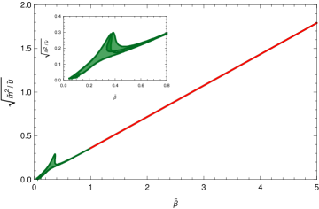
Figure 1: Comparison of the Planck data with the slow-roll result of the MNI single-field inflationary potential (1) with the specific choice for the constant term given in Eq. (2b), for $N=55$. The best choice for the parameters is that located inside the green region. The red line corresponds to fitted line starting from the origin. In the inset we report the comparison for small $\beta$ of the best acceptance regions (for $V_{2}$ and $V_{3}$).

II.2 Unification of Scales

Based on the slow-roll analysis discussed above, one can fix almost all parameters of the MNI (1) potential, and there is only a single free parameter left. In this subsection, we show how this remaining free parameter can be determined by requiring a kind of unification of all scales at the Grand Unification Theory (GUT) scale $k=2\times 10^{16}$ GeV.

The relation $u\beta^{2}/m^{2}>1$ holds. The dimensionless ratio $a=u\beta^{2}/m^{2}$ is found to have the following value

$$a=\frac{\tilde{u}\tilde{\beta}^{2}}{\tilde{m}^{2}}\approx\left(\frac{0.70}{0.26}\right)^{2}\approx 7.24\,,$$ (6)

as extracted from the data of Fig. 1. We emphasize that the result (6), valid at large $\beta$, do not depend on the constant term $V_{0}$, as it is highly desirable.

One can choose a particular point of that straight line where one finds the explicit mass of the MNI model,

$$\tilde{\beta}\approx 270\hskip 14.22636pt\to\hskip 14.22636ptm\sim 7\times 10^{15}{\mathrm{GeV}}\,,$$ (7)

in the the range of the cosmological scale, i.e., $k_{{\mathrm{cosmo}}}\sim 10^{15}-10^{16}$GeV and close to the GUT scale. In this case the dimensionless ratio $a$ again has the value $a\approx 7.24$. One cannot choose larger value for $\tilde{\beta}$ because then the explicit mass would be larger than the typical energy scale of the system, i.e., the cosmological scale. Thus, our choice is a maximum for $\tilde{\beta}$.

With this particular choice $\tilde{\beta}\approx 270$, the initial value for the VeV of the field is around $0.02\,\,m_{p}$ (see Fig. 2).

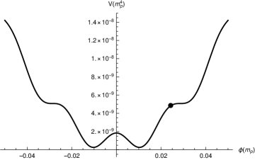
Figure 2: The MNI potential (denoted in the text as $V_{2}$) at the GUT scale. The black blob denotes the initial value of the VeV in the inflationary period.

Thus, we would like to emphasize that the MNI potential (1) requires no large field values in the very beginning of the cosmic inflation, and so, it is more reliably supported by GUT motivated model building rather than typical large-field inflationary models, where one has to assume very large initial value for the VeV of the field ($4-20\,\,m_{p}$). In addition, the initial value for the VeV of the MNI model is again in the range of the GUT scale. Therefore, by the choice $\tilde{\beta}\approx 270$ one is somehow able to unify all scales.

Finally, one should mention the following. If one would like to take into account all consequences of the quantum fluctuations of the inflaton field over inflation (where the rolling down of the VeV is basically considered as a classical process), one has to consider the RG running where the running scale is associated to the slowly rolling field itself lyth . This can be done in a reliable manner if the initial value for the VeV is around the momentum scale (which otherwise has been used as the scale for RG running) typical for inflation which is the GUT scale (or cosmological scale). The MNI model (1) with the dimensionless frequency $\tilde{\beta}\approx 270$ fulfills the required criteria.

III Electroweak Scale

There is a strong interest to find a link between these scalar fields of the Higgs and inflationary physics higgs_inflation_2_1 ; higgs_inflation_2_2 ; higgs_inflation_2_3 ; higgs_inflation_2_4 ; higgs_inflation_1_2 ; higgs_inflation_1_1 ; higgs_inflation_1_3 ; higgs_inflation_1_4 ; higgs_inflation_1_7 ; higgs_inflation_1_6 ; higgs_inflation_1_5 . The Standard Model (SM) Higgs field is an SU(2) complex scalar doublet with four real components, and the underlying symmetry of the electroweak sector is $SU(2)_{L}\times U(1)_{Y}$, thus, the SM Higgs Lagrangian reads as

$${\cal L}=(D_{\mu}\phi)^{\star}(D^{\mu}\phi)-V(\phi)-\frac{1}{2}{\rm Tr}\,({F}_{\mu\nu}{F}^{\mu\nu})$$ (8)

with

$$V=\mu^{2}\phi^{\star}\phi+\lambda(\phi^{\star}\phi)^{2}$$ (9)

and

$$D_{\mu}=\partial_{\mu}+ig{\bf T}\cdot{\bf W}_{\mu}+ig^{\prime}y_{j}B_{\mu},$$ (10)

where the vacuum expectation of the Higgs field is either at zero field for $\mu^{2}>0$ or at $\sqrt{\phi^{\star}\phi}=\sqrt{-\mu^{2}/(2\lambda)}=v/\sqrt{2}$ for $\mu^{2}<0$ with $v=246$ GeV known from low-energy experiments. The field can be parametrized around its ground state, where the unitary phase can be dropped by choosing an appropriate gauge. As a consequence of the Brout-Englert-Higgs mechanism englert_brout ; higgs , three degrees of freedom of the Higgs scalar field (out of the four) mix with weak gauge bosons. The remaining degree of freedom becomes the Higgs boson discovered at CERN’s Large Hadron Collider ATLAS ; CMS . The complete Lagrangian for the Higgs sector of the SM with the single real scalar field $h$ reads

$${\cal L}=\frac{1}{2}\partial_{\mu}h\partial^{\mu}h-\frac{1}{2}M^{2}_{h}h^{2}-\frac{M^{2}_{h}}{2v}h^{3}-\frac{M^{2}_{h}}{8v^{2}}h^{4}\\ +\left(M^{2}_{W}W^{+}_{\mu}W^{-\,\mu}+\frac{1}{2}M^{2}_{Z}Z_{\mu}Z^{\mu}\right)\left(1+2\frac{h}{v}+\frac{h^{2}}{v^{2}}\right),$$ (11)

where $M_{h}=\sqrt{-2\mu^{2}}=\sqrt{2\lambda v^{2}}$. The measured value for the Higgs mass $M_{h}=125.6\,{\mathrm{GeV}}$ implies $\lambda=0.13$. Incidentally, we note that the latter value is close to the predicted value based on an assumption of the absence of new physics between the Fermi and Planck scales and the asymptotic safety of gravity shapo_wett .

Extrapolating the SM of particle physics up to very high energies leads to an interpretation of the Higgs boson as the inflaton. Therefore, the most “economical” choice would be to use the same scalar field for Higgs and inflationary physics. The action can be defined either in the Jordan frame in which some function of the scalar field multiplies the Ricci scalar $R$, or in the Einstein frame in which the Ricci scalar is not multiplied by a scalar field jordan_einstein . To perform the slow-roll study, the action is usually rewritten in the Einstein frame and it takes the form for the case of minimal coupling to gravity,

$$S=\int d^{4}x\sqrt{-g}\left[\dfrac{m_{p}^{2}R}{2}-\frac{1}{2}g^{\mu\nu}\,\partial_{\mu}\phi\,\partial_{\nu}\phi-V(\phi)\right]\,,$$

$$V\equiv\dfrac{\lambda}{4}\left(\phi^{2}-v^{2}\right)^{2}=\dfrac{M^{2}_{h}}{8v^{2}}\left(\phi^{2}-v^{2}\right)^{2},$$ (12)

where the metric tensor being denoted by $g^{\mu\nu}$, $\sqrt{-g}\equiv\sqrt{-{\rm det}\,g}$ while $\phi\equiv h$ and $V$ is the quartic-type double-well scalar potential of (11),

$$V(\phi)=\frac{\lambda}{4}v^{4}-\frac{1}{2}\lambda v^{2}\phi^{2}+\frac{\lambda}{4}\phi^{4}\,.$$ (13)

where the field variable is shifted as $h\to h+v$. The case of non-minimal inflation is discussed in Appendix B.

Another proposal to build up the scalar sector is the Higgs inflation from false vacuum with minimal coupling to gravity where the SM Higgs potential is extended and assumed to develop a second (or more) minimum higgs_inflation_2_1 ; higgs_inflation_2_2 ; higgs_inflation_2_3 ; higgs_inflation_2_4 . The difficulty is to achieve an exit from the inflationary phase: one may introduce new fields, but than the attractive minimality of the model would be lost.

Another possible drawback of the Higgs-inflaton potential to its applicability is that the measured Higgs mass is close to the lower limit, $126$ GeV, ensuring absolute vacuum stability within the SM NNLO_stability . However, it was also shown bezrukov_rubio_shapo that traditional Higgs inflation can be possible within a minimalistic framework even if the SM vacuum is not completely stable. Various polynomial Higgs potentials have been studied by functional RG higgs_frg_1 ; higgs_frg_2 and reported no stability problems.

All versions of the MNI model studied by us contain two adjustable parameters (the ratio $u/m^{2}$ and the frequency $\beta$) and a normalization (the field-independent terms has been fixed by us). The Taylor expansion of the MNI model (1) recovers the SM Higgs potential (13) up to quartic terms and the parameters can be related:

$$V_{\rm MNI}\approx V_{0}+\frac{1}{2}(m^{2}-u\beta^{2})\phi^{2}+\frac{1}{24}u\beta^{4}\phi^{4}+{\mathcal{O}}(\phi^{6})\,,$$ (14)

so that

$$\lambda v^{2}\equiv(u\beta^{2}-m^{2}),\hskip 11.38092pt\lambda\equiv\frac{1}{6}u\beta^{4}.$$ (15)

Thus the MNI model (1) can be considered as an UV completion of the SM Higgs potential. Further details of the UV completion is shown in Appendix C. The measurable quantities are related to the parameters of the model according to the following relations:

$$M_{h}\equiv m\sqrt{2\left(\frac{u\beta^{2}}{m^{2}}-1\right)},\hskip 11.38092ptv\equiv\frac{1}{\beta}\sqrt{\frac{6(u\beta^{2}/m^{2}-1)}{u\beta^{2}/m^{2}}}.$$ (16)

Their low-energy/IR values are given at the electroweak scale by

$$M_{h,{\mathrm{IR}}}=125\,\,{\mathrm{GeV}},\hskip 14.22636ptv_{{\mathrm{IR}}}=245\,\,{\mathrm{GeV}}\,,$$ (17)

at the scale $k_{{\mathrm{IR}}}\sim 250{{\mathrm{GeV}}}$.

Notice that taking into account higher order terms in Eq. (14) gives rise to results consistent with (16), as discussed in Appendix D.

Let us note, that the Higgs mass and VeV defined by (16) can be calculated also at the cosmological scales. For example, in the large $\tilde{\beta}$ region the slow-roll study produces values for the Higgs mass and VeV in the same order of magnitude which serves as a high-energy/UV scale

$$M_{h,{\mathrm{UV}}}\sim \;v_{{\mathrm{UV}}}\sim 10^{15}\,{\mathrm{GeV}}\,,$$ (18a)

$$m_{{\mathrm{UV}}}\sim \;10^{15}{\mathrm{GeV}},\hskip 5.69046pt\beta_{{\mathrm{UV}}}\sim 10^{-15}\,{\mathrm{GeV}}^{-1}\,,$$ (18b)

at the scale $k_{{\mathrm{UV}}}\sim 10^{15}{{\mathrm{GeV}}}$. These need to be scaled down (by orders of magnitude) to their measured values at the electroweak scale (17). The integration of high-energy modes is a well-known method which provides us this scaling down by the successful integration of the field fluctuations. Therefore, let us discuss the integration of the high-energy modes in the MNI model in the post-inflation period.

IV Mode Integration

In principle, a comprehensive study of the integration of high-energy modes requires an accurate treatment of gauge and fermion fields and not just a single scalar potential. However, the MNI model has a very important feature, namely it contains a periodic and a quadratic self-interaction term (apart from the trivial constant term). It allows to perform explicitly, in an easy way, the integration of modes up to the electroweak scale. The explanation is the following. The integration of modes is done by solving the RG flow differential equation where not the action but its Hessian (second derivative) appears on the one side eea_rg_1 ; eea_rg_2 . So, even if the scalar field couples to any gauge or fermion fields in the action (which are not higher than quadratic in the scalar field), the Hessian remains periodic in the scalar sector. Therefore, it represents a reliable approximation if one looks for the solution of the equation among scalar periodic functions and neglect the effect of other fields.

IV.1 Flow Equation for the Potential

A field theory closely related to the MNI model (1), namely, the massive sine-Gordon scalar model, was extensively studied in $d=2$ dimensions by functional RG method msg_lpa_1 ; msg_lpa_2 ; msg_lpa_3 ; msg_beyond_lpa . Here, we consider $d=4$ dimensions. The procedure, standard in RG approaches, consists in eliminating the high-energy modes by integrating them. This gives an equation for the flow of the potential, and the general fact is that this equation is a functional one. When the high-energy modes are integrated out, the potential therefore becomes scale-dependent, $V\to V_{k}$, where with the symbol $V_{k}$ we denote that the modes with momenta larger than $k$ have been integrated out. To determine the dependence on the scale $k$ one has to solve the RG flow equation which has the following form at the level of the local potential approximation where higher-order derivatives of the field are neglected eea_rg_1 ; eea_rg_2 ,

$$k\partial_{k}{V_{k}(\varphi)}=\frac{1}{2}\int\frac{d^{d}p}{(2\pi)^{2}}\,\frac{k\partial_{k}R_{k}}{R_{k}+p^{2}+\partial^{2}_{{\phi}}V_{k}}\,,$$ (19)

where $R_{k}=R_{k}(p^{2})$ is a cut-off function, which in the functional RG jargon is called regulator function. Then, one can turn to dimensionless quantities, denoted by a tilde superscript as written in Eqs. (II.1). The RG flow equation becomes

$$\left(d-\frac{d-2}{2}\tilde{\varphi}\partial_{\tilde{\varphi}}+k\partial_{k}\right)\tilde{V}_{k}(\tilde{\varphi})=\hskip 56.9055pt$$

$$-\alpha_{d}\int_{0}^{\infty}dy\,\frac{r^{\prime}\,\,y^{\frac{d}{2}+1}}{[1+r]\,y\,+\partial^{2}_{\tilde{\phi}}\tilde{V}_{k}}\,,$$ (20)

with $\alpha_{d}=\Omega_{d}/(2(2\pi)^{d})$ and $\Omega_{d}=2\pi^{d/2}/\Gamma(d/2)$, where it is intended we have to put $d=4$. Moreover $r(y)$ is the dimensionless regulator defined by $r(y)=R_{k}(p^{2})/p^{2}$, with $y=p^{2}/k^{2}$ and $r^{\prime}=dr/dy$. The integral in the right-hand-side of Eq. (IV.1) can be performed analytically by the appropriate choice of the regulator function, for example by using $r(y)=(1/y-1)\Theta(1-y)$. The results should be independent on the particular regulator which has been chosen: this issue has been discussed in considerable detail in the functional RG literature, so we just pass to present our results.

Two comments are anyway in order: i) the mode integration procedure above described give the same results for all variants of the MNI model ($V_{1}$, $V_{2}$ and $V_{3}$) since the derivation with respect to the field eliminates any dependence on field-independent terms; ii) the results presented in Fig. 3 and Fig. 4, and the UV-insensitivity property, do not depend on the choice of the regulator.

Our results can be summarized by observing that one finds two phases controlled by the dimensionless quantity $\tilde{u}_{k}\tilde{\beta}_{k}^{2}/\tilde{m}_{k}^{2}$, which tends to a constant in the IR limit. In the ($Z_{2}$) symmetric phase the magnitude of this constant is arbitrary (and depends on the initial conditions), but always smaller than one, i.e., $\lim_{k\to 0}|\tilde{u}_{k}\tilde{\beta}_{k}^{2}/\tilde{m}_{k}^{2}|<1$ (see the blue lines of Fig. 3).

In the spontaneously broken (SSB) phase, the IR value of the magnitude of the ratio is exactly one (independently of the initial values) which serves as an upper bound, see green lines of Fig. 3. The black line separates the two phases.

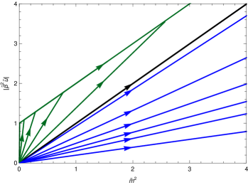
Figure 3: Flow of the MNI model showing two phases separated by a black line with a unit slope. The blue lines corresponds to the symmetric phase, while the green lines correspond to the SSB phase.

In other words, trajectories in the SSB phase (green lines) merge into a master trajectory (green line parallel to the black one) of Fig. 3 which implies

$$\bar{u}_{k}\tilde{\beta}_{k}^{2}=1+\tilde{m}_{k}^{2}\,,$$ (21)

and it results in the following scaling:

$$\frac{\bar{u}_{k}\tilde{\beta}_{k}^{2}}{\tilde{m}_{k}^{2}}-1=\frac{1}{\tilde{m}_{k}^{2}}=\frac{k^{2}}{m^{2}_{{\mathrm{UV}}}}.$$ (22)

This scaling relation is valid when the running is determined by the master trajectory which, apart from the very beginning of the running, is always the case in the SSB phase. We observe that Eq. (22) has been obtained with a non-perturbative approach for the MNI potential (1), but one may expect that it is valid for other classed of inflationary potentials, as we are going to discuss in Section IV.2 and V. However, the MNI potential (1) is well suited to find Eq. (22) in a particularly transparent way.

Eq. (22) can be used to determine the IR value of the Higgs mass and VeV from the UV initial conditions (18a) and compared to the known results of (17). Indeed by substituting (22) into (16) and assuming running parameters $\tilde{u}_{k}\tilde{\beta}_{k}^{2}/\tilde{m}_{k}^{2}=u_{k}\beta^{2}/m^{2}$, one gets

$$M_{h}(k)=m_{{\mathrm{UV}}}\sqrt{2\left(\frac{\tilde{u}_{k}\tilde{\beta}_{k}^{2}}{\tilde{m}_{k}^{2}}-1\right)}.$$ (23)

Now, one uses Eq. (22) and obtains

$$M_{h}(k)=m_{{\mathrm{UV}}}\,\sqrt{2}\,\sqrt{\frac{k^{2}}{m_{{\mathrm{U}}V}^{2}}}=\sqrt{2}\,\cancel{m_{{\mathrm{UV}}}}\frac{k}{\cancel{m_{{\mathrm{UV}}}}}=\sqrt{2}k,$$ (24)

where the cancellation of the UV mass has been made evident. We observe, for absolute clarity, that this property does not depend of the specific form of the flow (IV.1), but is a consequence of the fact that the ratio $u\beta^{2}/m^{2}$ is constant.

Similarly, one gets

$$v(k)=\frac{1}{\beta_{{\mathrm{UV}}}}\sqrt{\frac{6(\tilde{u}_{k}\tilde{\beta}_{k}^{2}/\tilde{m}_{k}^{2}-1)}{\tilde{u}_{k}\tilde{\beta}_{k}^{2}/\tilde{m}_{k}^{2}}}=\frac{\sqrt{6}k}{m_{{\mathrm{UV}}}\beta_{{\mathrm{UV}}}}\,,$$ (25)

which has important consequences. Since $k_{{\mathrm{IR}}}$ = 250 GeV, it provides the required IR values (17), at least the same order, in accordance with measurements. Furthermore, the IR values for the Higgs mass becomes independent of the UV initial parameter (see Fig. 4).

We conclude this Section by observing that the (dimensionful) Higgs mass has a weak RG running in the framework of perturbative RG in the SM Peskin . We are in agreement with this fact, since in our model the (dimensionful) mass $m$ has no running at all. However, with the non-perturbative approach followed in the present paper, the Higgs mass is an effective mass and it is not the explicit mass $m$. This is shown in Fig. 4 clearly demonstrating the linear dependence of the effective Higgs mass obtained using the MNI model (1).

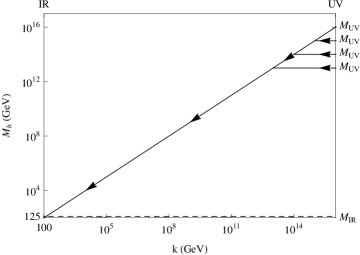
Figure 4: Flow of the Higgs mass from the cosmological (UV) scale to the electroweak (IR) scale obtained from the study of the MNI model. The trajectories merge into a single line showing UV insensitivity.

IV.2 Comments on Universality

The previous derivation show that the details at cosmological scale do not influence the quantities at the electroweak scale. This property manifests itself through the cancellation of the parameter $m$ of the MNI determined at cosmological scale using PLANCK data. In practice, whatever is the value of $m$ and $\beta$ at cosmological scale, one gets the same value for the Higgs mass, which depends only on the chosen energy scale at electroweak, IR scale, which we can denote by $k_{\rm ew}$. This is evident from the universality of the flow, as depicted in Fig. 4, where all trajectories flow into the same point. Our analysis also shows that the initial condition, which we may denote by $k_{\rm start}$, chosen as starting point for the mode integration, also does not play a role.

Now, the question that naturally emerges is the following: is this property specific to the MNI alone or not? Before answering, we pause to comment that in general, the MNI is very suited to show the property of independence of the Higgs mass from the initial conditions and from the values of the parameters at cosmological scale, since the mode integration can be performed straightforwardly using known results from field theory. Actually, the cancellation of the mass $m$ emerge naturally and with a minimally simple calculation. However, this usefulness of the MNI does not imply that it is the only model exhibiting such features. Indeed, we expect that other two-parameter inflationary model with $Z_{2}$ symmetry will give the same results. The reason for such expectation is three-fold: from one side, during the mode integration, all powers of the field are generated and the interplay of the minima depends on these powers. Such a generation is not specific of the MNI model and will be exhibited by other models: actually, we can say the opposite, namely that if the model has an Higgs mass depending on the parameters determined from cosmological data, then most probably it could be characterized as unphysical. So, this led to conclude that extending an inflationary model towards low energies should produce the same Higgs mass provided that $k_{ew}$ is fixed, and the MNI is in our opinion just a simple model showing this result. From the other side, it is well known that mode integration makes the potential tend to a convex form starting from a concave one, and this is in agreement with $M_{h}(k_{ew})/m\ll 1$. Finally, it should be noted that for scalar theories in four dimensions, the only relevant and marginal couplings are the quadratic and the quartic one respectively. When considering more complicated functional forms for the potential, the scaling arguments cannot be straightforwardly applied, and the irrelevance of higher-order field terms is not evident from the $\beta$-functions. Even in this case, the simple scaling arguments are expected to hold, and so we expect the irrelevance from the UV conditions to hold even for different UV completions.

V Conclusions and Outlook

A good candidate for an inflationary potential should fulfill the following conditions, (i) have an as-simple-possible functional form (with the smallest possible number of parameters), (ii) provide the best agreement with observations, (iii) be as “economical” as possible in term of the formulation of the theory. In this paper, we propose the extended version of the massive sine-Gordon theory as an inflationary potential and we refer to it as the massive Natural Inflation (MNI) model. We show that adding the mass term to the periodic potential produces a remarkably improved agreement with the Planck results. We attribute such improvement to the fact that it has infinitely many minima, but they are non-degenerate and with tunable controllable energy difference, providing a way to be as much as possible both “$\phi^{2}$ and not-$\phi^{2}$”. The crucial point emerging from a careful analysis of different potentials is that the inflationary potential should have a concave region, and the mass term in the MNI potential add such an overall convexity in presence of the many minima.

To explore the issue of the convexity, we used the known renormalization group (RG) results for the MNI model, extending them to $d=4$, to perform explicitly the mode integration. We then determined the phase diagram associated to the running determined by the slow-roll conditions having in mind the post-inflation period. The obtained values for the ratio $|\tilde{u}_{k}\tilde{\beta}_{k}^{2}/\tilde{m}_{k}^{2}|$ are found in the phase of spontaneous symmetry breaking (above the critical line). Thus, the study of the MNI model shows that slow-roll conditions represent strong constraints on the RG running i.e., it stays in its broken phase. Moreover, the mode integration produces a convex (dimensionful) potential in agreement with the theoretical requirement of the convexity of the effective potential.

In conclusion, we introduced a model for cosmological inflation, based on a UV completion of the Higgs potential, which has the following properties:

• it works at cosmological level, and its parameters can be fixed from PLANCK and BICEP2 experimental data. (This property is shared with many other models which are consistent with available data at the cosmological scale, but still constitutes an important consistency check of our model.)

• Our model also works at the electroweak scale which means its parameter can be fixed by comparison with experimental data. This property, by contrast, is not shared by other UV-admissible models which work at the cosmological scale. Within our assumptions, the Higgs mass is found to be independent of the parameters found at the cosmological scale.

• We argue that these properties are shared by other two-parameter inflationary models, but our model provides an ideal framework to explicitly show it in a straightforward way.

We conclude that the model is valid both at cosmological and electroweak scales.

Finally, we comment on the consequences of our results related to three major issues of inflationary cosmology which have and are intensely discussed. The first concerns the identification of the inflaton with the Higgs field, i.e., whether the inflationary potential can be be extended to electroweak scale in a reliable way. The second is whether the high-energy properties of the theory affect or not the low-energy ones: when there is not such influence, one talks about UV-insensitivity fumagalli . The third issue is related to the fact that many inflationary models can be and have been proposed encyc , so that it may be asked whether and how the correct model should be chosen. The fact that one has to choose an ad hoc potential with a fine tuning of its parameters and of the initial conditions is certainly an argument against inflationary scenarios. Our paper brings a contribution to this on-going discussion, since our results suggest that the answer to first question is “yes”, in the sense that the results for the Higgs mass does not depend on the values of the model parameter at cosmological scale and that one can explicitly build a model valid at cosmological and electroweak scale. The answer to second question, looking at the results of the MNI analysis presented in the present paper, is that there is UV-insensitivity, as the MNI clearly shows with the cancelation of the mass $m$ at cosmological scale in determining $M_{h}(k_{ew})$. For the third question we conclude “no”, in the sense that other models with non-fine tuned initial conditions share the same properties. The affirmative answer to the first question supports Higgs inflationary models. If one were to insist that a single specific model, with uniquely determined parameters, should explain the physical properties at all scales, then the model-independence and UV-insensitivity could be considered as an argument against Higgs inflation. However, if one is taking an approach like the renormalization group approach à la Wilson, then the model-independence (and UV-insensitivity) is not only desirable, but, in a sense, required.

Summing all the radiative corrections to the quartic Higgs potential (and of course having at disposal more experimental data) could shed light on this apparent contradiction and on the form of the effective action at the cosmological scale. However, we think that the top-down approach based on a guessed action at high-energies may give very useful informations to clarify the properties that the UV action should have in order to fulfill the requested requirements at all scales. This approach is opposite to the more standard one bottom-up, which starts from the low-energy properties and tries to obtain the action at high-energies, and it may give complementary information. This is one of the reasons for which we hope that the results presented in this paper may contribute to the discussion on the validity of specific inflationary models.

In conclusion, we found a class of MNI models which show UV insensitivity and can act as viable candidates for an inflaton mechanism, via integration of the high-energy modes. While it will be impossible, from low-energy experiments alone, to determine which is the correct one, one could confirm that only rather moderate extensions of the Standard Model (in this case, the addition of periodic terms) would be required for a consistent extrapolation to very high energy scales, the latter being of cosmological relevance.

Acknowledgements.— This work was supported by the János Bolyai Research Scholarship of the Hungarian Academy of Sciences and by the ÚNKP-17-3 New National Excellence Program of the Ministry of Human Capacities. Useful discussions with F. Bianchini, G. Gori, J. Rubio, Z. Trocsanyi and G. Somogyi are gratefully acknowledged. Support from the National Science Foundation (Grant PHY–1710856) also is being acknowledged. Financial support by the CNR/MTA Italy–Hungary 2019–2021 Joint Project ”Strongly interacting systems in confined geometries” is gratefully acknowledged.

Appendix A Inflationary predictions

In this appendix we discuss the applicability of the Natural Inflation (NI) and the Massive Natural Inflation (MNI) potentials for cosmology. The slow-roll parameters ($\epsilon$, $\eta$, $n_{s}$, $r$) of the NI model reads as

$$\epsilon= \frac{\tilde{\beta}^{2}}{2}\cot^{2}\left(\frac{\tilde{\beta}\tilde{\phi}}{2}\right),\hskip 11.38092pt\eta=\frac{\tilde{\beta}^{2}}{2}\frac{\cos(\tilde{\beta}\tilde{\phi})}{\sin^{2}\left(\frac{\tilde{\beta}\tilde{\phi}}{2}\right)},$$

$$N= -\frac{2}{\tilde{\beta}^{2}}\log\cos\left(\frac{\tilde{\beta}\tilde{\phi}}{2}\right)\Big{|}^{\tilde{\phi}_{i}}_{\tilde{\phi}_{f}}$$

$$n_{s}-1 \approx\tilde{\beta}^{2}\left[1-2\sin^{-2}\left(\frac{\tilde{\beta}\tilde{\phi}}{2}\right)\right],\,\,\,\,\,\,r\approx 8\tilde{\beta}^{2}\cot\left(\frac{\tilde{\beta}\tilde{\phi}}{2}\right)$$

which imply the relation $n_{s}-1+\frac{r}{4}=-\tilde{\beta}^{2}$ which is very similar to that of obtained for the quadratic monomial potential but having a dependence on the frequency $\tilde{\beta}$, thus, it appears as an additional parameter which can be tuned ($\tilde{\beta}\sim 0.15$) to achieve a better agreement with the Planck data, see orange line segments of Fig. 5.

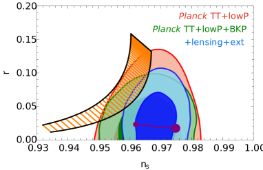
Figure 5: CMBR parameters, i.e., scalar tilt $n_{s}$ and tensor-to-scalar ratio $r$ derived (i) for the Natural Inflation model for various frequencies (orange line segments) and (ii) for the MNI model with fixed ratio $\tilde{u}/\tilde{m}^{2}\sim 1/(0.22)^{2}$ and frequency $\tilde{\beta}\sim 0.3$ (purple line segment). Both are compared to results of the Planck mission planck_1 ; planck_2 ; planck_3 where dark color regions stand for 95% CL and light color regions correspond to 68% CL.

The slow-roll parameters of the MNI model (2a),

$$\epsilon= \frac{1}{2}\left(\frac{\frac{\tilde{u}}{\tilde{m}^{2}}\tilde{\beta}\sin(\tilde{\beta}\tilde{\phi})+\tilde{\phi}}{\frac{\tilde{u}}{\tilde{m}^{2}}\left[1-\cos(\tilde{\beta}\tilde{\phi})\right]+\frac{1}{2}\tilde{\phi}^{2}}\right)^{2}$$ (26)

$$\eta= \frac{\frac{\tilde{u}}{\tilde{m}^{2}}\tilde{\beta}^{2}\cos(\tilde{\beta}\tilde{\phi})+1}{\frac{\tilde{u}}{\tilde{m}^{2}}\left[1-\cos(\tilde{\beta}\tilde{\phi})\right]+\frac{1}{2}\tilde{\phi}^{2}}$$ (27)

$$N= -\int_{\tilde{\phi}_{i}}^{\tilde{\phi}_{f}}d\tilde{\phi}\frac{\frac{\tilde{u}}{\tilde{m}^{2}}\left[1-\cos(\tilde{\beta}\tilde{\phi})\right]+\frac{1}{2}\tilde{\phi}^{2}}{\frac{\tilde{u}}{\tilde{m}^{2}}\tilde{\beta}\sin(\tilde{\beta}\tilde{\phi})+\tilde{\phi}}$$ (28)

depend on the ratio $\tilde{u}/\tilde{m}^{2}$ and the frequency $\tilde{\beta}$. The inclusion of the explicit mass term ($\frac{1}{2}m^{2}\phi^{2}$) in the periodic (i.e., NI) potential improves the inflationary predictions of the model, see Fig. 5.

Appendix B Non-minimal Inflation

In this appendix we discuss the case of a large non-minimal coupling to gravity higgs_inflation_1_1 ; higgs_inflation_1_2 ; higgs_inflation_1_3 ; higgs_inflation_1_4 ; higgs_inflation_1_5 ; higgs_inflation_1_6 ; higgs_inflation_1_7 , where the interpretation of the Higgs boson as the inflaton results in the following action in the Jordan frame

$$S=\int d^{4}x\sqrt{-\bar{g}}\frac{m_{p}^{2}}{2}\left[F(\tilde{h})\bar{R}-\bar{g}^{\mu\nu}\partial_{\mu}\tilde{h}\partial_{\nu}\tilde{h}-2U(\tilde{h})\right]\,,$$

$$F(h)=1+\xi\tilde{h}^{2},\hskip 5.69046ptU(\tilde{h})=m_{p}^{2}\dfrac{\lambda}{4}\left(\tilde{h}^{2}-\dfrac{v^{2}}{m^{2}_{p}}\right)^{2}\,,$$ (29)

where $\tilde{h}$ is the dimensionless Higgs scalar ($h=m_{p}\tilde{h}$), $\xi$ is a new parameter and $\bar{g}^{\mu\nu}$ is the metric in the Jordan frame. Of course, by convention, $\sqrt{-\bar{g}}\equiv\sqrt{-{\rm det}\,\bar{g}}$, while $U(\tilde{h})$ is the dimensionless quartic-type double-well scalar potential with a $Z_{2}$ symmetry, equivalent to the SM Higgs potential of (11). In order to show this one has to (i) introduce a dimensionful field variable, (ii) replace the quartic self-coupling by the Higgs mass, i.e., $\lambda=M^{2}_{h}/(2v^{2})$ as is indicated below Eq. (11), and (iii) shift the field variable as $h\to h+v$.

To perform the slow-roll study, the action is usually rewritten in the Einstein frame and it takes the form

$$S=\int d^{4}x\sqrt{-g}\left[\dfrac{m_{p}^{2}R}{2}-\frac{1}{2}g^{\mu\nu}\,\partial_{\mu}\phi\,\partial_{\nu}\phi-V(\phi)\right]\,,$$

$$V\equiv m_{p}^{2}\dfrac{U}{F^{2}},\hskip 5.69046pt\dfrac{d\phi}{d\tilde{h}}=m_{p}\dfrac{\sqrt{1+\xi(1+6\xi)\tilde{h}^{2}}}{1+\xi\tilde{h}^{2}}\,,$$ (30)

where the metric tensor being denoted by $g^{\mu\nu}$. For $\xi\neq 0$, the Higgs-$\xi$ inflaton potential reads

$$V(\phi)=\frac{m_{p}^{4}\lambda}{4\xi^{2}}\left[1-\exp\left(-\sqrt{\frac{2}{3}}\dfrac{\phi}{m_{p}}\right)\right]^{2},$$ (31)

which is considered as a zero parameter model since the overall factor of the potential is entirely determined by the amplitude of the CMBR anisotropies. In the framework of this inflationary scenario, one needs to take extra precautions in order not to violate perturbative unitarity.

Appendix C UV completion

Alternatively, the MNI-type UV completion of the SM Higgs potential can be formulated as

$$V=\frac{1}{2}M^{2}\phi^{\star}\phi+u[\cos(b\sqrt{\phi^{\star}\phi})-1]\,,$$ (32)

which recovers the scalar potential in (8) after its Taylor expansion with $\mu^{2}\equiv 1/2\,\,(M^{2}-ub^{2})$ and $\lambda\equiv\tfrac{1}{24}\,\,ub^{4}$. Performing the same parametrization of the field used in order to get from (8) to (11) one finds

$$V=\frac{1}{2}\,\,\frac{M^{2}}{2}(h+v)^{2}+u\left[\cos\left(\frac{b}{\sqrt{2}}(h+v)\right)-1\right],$$ (33)

which is identical (apart from constant terms) to the MNI model (1) after shifting the field by a constant $h+v\to\phi$ and introducing $m^{2}\equiv M^{2}/2$ and $\beta\equiv b/\sqrt{2}$. This validates that the MNI model is a suitable extension of the SM Higgs potential. The broken symmetric case corresponds to parameters where $1<u\beta^{2}/m^{2}=ub^{2}/M^{2}$, i.e., where $\mu^{2}<0$.

Appendix D Effect of higher order terms on the vacuum expectation value

The vacuum expectation value (VEV) $v$ is defined by the value of the field ($\phi$) at the minima of the potential:

$$V(\phi=v)=\min(V).$$ (34)

In our case the VEV is the closest solutions to zero of the equation

$$\left.\frac{dV}{d\phi}\right|_{\phi=v}=0\,,$$ (35)

which for the MNI model writes as

$$m^{2}v-\beta u\sin(\beta v)=0\,.$$ (36)

One obtains

$$\sqrt{\frac{u\beta^{2}/m^{2}-1}{u\beta^{2}/m^{2}}}=\sqrt{1-\frac{\sin(\beta v)}{\beta v}}\,.$$ (37)

The left hand side is smaller than one and we remind we are looking for the solutions for $v$ which is the closest to zero. Thus the calculations with only the first order of the right hand side (which is equivalent to keep only the $\phi^{n}$ terms, with $n\leq 4$, in the potential) is a reasonable approximation, see Fig. 6.

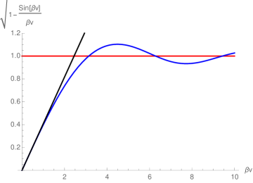
Figure 6: The first order approximation of the right hand side of (37) (black line). T he red line is the maximum value of the left hand side of (37) while the blue curve is the exact result.

We conclude that taking into account the higher terms changes the scaling of the VEV, which anyway stays very close to the first order approximation written in the paper.

References

- (1) A. H. Guth, Phys. Rev. D 23, 347 (1981).
- (2) A. Linde, Phys. Lett. B 108, 389 (1982).
- (3) A. Albrecht and P. J. Steinhardt, Phys. Rev. Lett. 48, 1220 (1982).
- (4) J. Earman and J. Mosterin, Philos. Sci. 66, 1 (1999).
- (5) P. J. Steinhardt, Sci. Am. 304, 18 (2011).
- (6) F. Bezrukov, J. Rubio, and M. Shaposhnikov, Phys. Rev. D 92, 083512 (2015).
-
(7)
Javier Rubio,
arXiv:1807.02376 - (8) J. Borchardt, H. Gies, and R. Sondenheimer, Eur. Phys. J. C 76, 472 (2016).
- (9) A. Jakovac, I. Kaposvari, and A. Patkos, Mod. Phys. Lett. A 32, 1750011 (2017).
- (10) V. Branchina and E. Messina, Phys. Rev. Lett. 111, 241801 (2013).
- (11) V. Branchina, E. Messina, A. Platania, JHEP 1409, 182 (2014); E. Bentivegna, V. Branchina, F. Contino, and D. Zappala, ibid. 1712, 100 (2017).
- (12) J. Martin, C. Ringeval, and V. Vennin, Encyclopaedia Inflationaris, Phys. Dark Univ. 5-6, 75 (2014).
- (13) P. Creminelli, D. Lopez Nacir, M. Simonovic, G. Trevisan, and M. Zaldarriaga, Phys. Rev. Lett. 112, 241303 (2014).
- (14) S. Coleman, Phys. Rev. D 11, 2088 (1975).
- (15) K. Freese, J. A. Frieman, and A. V. Olinto, Phys. Rev. Lett. 65, 3233 (1990).
- (16) K. Freese and W. H. Kinney, JCAP 03, 044 (2015).
- (17) C. P. Burgess, M. Cicoli, F. Quevedo, and M. Williams, JCAP 11, 045 (2014).
- (18) K. Yonekura, JCAP 10, 054 (2014).
- (19) K. Kohri, C. S. Lim, and C. M. Lin, JCAP 08 001 (2014).
- (20) T. Chiba, K. Kohri, PTEP 2014, 093E01 (2014).
- (21) L. Boyle, K. M. Smith, C. Dvorkin, and N. Turok, Phys. Rev. D 92, 043504 (2015).
- (22) I. P. Neupane, Phys. Rev. D 90, 123502 (2014).
- (23) J. B. Munoz and M. Kamionkowski, Phys. Rev. D 91, 043521 (2015).
- (24) C. Burgess and D. Roest, JCAP 06, 012 (2015).
-
(25)
I. Nandori,
arXiv:1108.4643 - (26) P. A. R. Ade et al. [Planck], Astron. Astrophys. 594, A20 (2016).
- (27) P. A. R. Ade et al. [Planck], Astron. Astrophys. 594, A13 (2016).
- (28) P. A. R. Ade et al. [BICEP2 and Keck Array], Phys. Rev. Lett. 116, 031302 (2016).
- (29) I. Nandori, S. Nagy, K. Sailer, and A. Trombettoni, Phys. Rev. D 80, 025008 (2009).
- (30) I. Nandori, Phys. Lett. B 662, 302 (2008).
- (31) S. Nagy, I. Nandori, J. Polonyi, and K. Sailer, Phys. Rev. D 77, 025026 (2008).
- (32) I. Nandori, Phys. Rev. D 84, 065024 (2011).
- (33) M. Postma, NIKHEF 53 (2009).
- (34) D. H. Lyth and A. Riotto, Phys. Rept. 314 1-146 (1999).
- (35) D. L. Bennett, H. B. Nielsen, and I. Picek, Phys. Lett. B 208, 275 (1988).
- (36) C. D. Froggatt, H. B. Nielsen, Phys. Lett. B 368, 96 (1996).
- (37) C. P. Burgess, V. Di Clemente, and J. R. Espinosa, JHEP 0201, 041 (2002).
- (38) G. Isidori, V. S. Rychkov, A. Strumia, and N. Tetradis, Phys. Rev. D 77, 025034 (2008).
- (39) F. Bezrukov and M. Shaposhnikov, Phys. Lett. B 659, 703 (2008).
- (40) F. Bezrukov and M. Shaposhnikov, JHEP 0907, 089 (2009).
- (41) C. P. Burgess, H. M. Lee, and M. Trott, JHEP 0909, 103 (2009).
- (42) J. L. F. Barbon and J. R. Espinosa, Phys. Rev. D 79, 081302 (2009).
- (43) A. De Simone, M. P. Hertzberg, and F. Wilczek, Phys. Lett. B 678, 1 (2009).
- (44) R. N. Lerner and J. McDonald, Phys. Rev. D 82, 103525 (2010).
- (45) G. F. Giudice and H. M. Lee, Phys. Lett. B 694, 294 (2011).
- (46) F. Englert and R. Brout, Phys. Rev. Lett. 13, 321 (1964).
- (47) P. W. Higgs, Phys. Rev. Lett. 13 508 (1964).
- (48) ATLAS Collaboration, Phys. Lett. B 710, 49 (2012).
- (49) CMS Collaboration, Phys. Lett. B 710, 26 (2012).
- (50) M. Shaposhnikov and C. Wetterich, Phys. Lett. B 683, 196 (2010).
- (51) M. Postma, M. Volponi, Phys. Rev. D 90 103516 (2014).
- (52) G. Degrassi, S. Di Vita, J. Elias-Miró, J. R. Espinosa, G. F. Giudice, G. Isidori, and A. Strumia, JHEP 08, 098 (2012).
- (53) C. Wetterich, Phys. Lett. B 301 90 (1993).
- (54) T. R. Morris, Int. J. Mod. Phys. A 9 2411 (1994).
- (55) M. E. Peskin and D. V. Schroeder, An introduction to quantum field theory (Reading, Addison-Wesley, 1995).
- (56) J. Fumagalli and M. Postma, JHEP 1605, 049 (2016).