Sequential Multiple Testing

Abstract

We study an online multiple testing problem where the hypotheses arrive sequentially in a stream. The test statistics are independent and assumed to have the same distribution under their respective null hypotheses. We investigate two procedures LORD and LOND, proposed by (Javanmard and Montanari, 2015), which are proved to control the FDR in an online manner. In some (static) model, we show that LORD is optimal in some asymptotic sense, in particular as powerful as the (static) Benjamini-Hochberg procedure to first asymptotic order. We also quantify the performance of LOND. Some numerical experiments complement our theory.

1 Introduction

Multiple testing is now a well-established area in statistics and arises in almost every scientific field (Dudoit and van der Laan, 2007; Dickhaus, 2014; Roquain, 2011). In this paper, we consider a scenario where infinitely many hypotheses $\mathcal{H}=(\mathbb{H}_{1},\mathbb{H}_{2},\mathbb{H}_{3},\dots)$ arrive sequentially in a stream with corresponding P-values $P_{1},P_{2},P_{3},\dots$, and we are required to decide whether we accept or reject $\mathbb{H}_{i}$ only based on $P_{1},\dots,P_{i}$. We propose to use the recent sequential multiple testing procedures of (Javanmard and Montanari, 2015) which control the FDR in an online manner, and study the asymptotic optimality properties of these methods in the context of sparse mixture asymptotically generalized Gaussian model (see Definition 1) which the normal model often used as benchmark in various works on multiple testing.

1.1 The risk of a multiple testing procedure

Consider a setting where we want to test an ordered infinite sequence of null hypotheses, denoted $\mathcal{H}=(\mathbb{H}_{1},\mathbb{H}_{2},\mathbb{H}_{3},\dots,$), where at each step $i$ we have to decide whether to reject $\mathbb{H}_{i}$ having access to only previous decisions. The test that we use for $\mathbb{H}_{i}$ rejects for large positive values of a statistic $X_{i}$. Throughout, we assume that test statistics are all independent. Denote the collection of the first $n$ hypotheses in the stream by $\mathcal{H}(n)=(\mathbb{H}_{1},\dots,\mathbb{H}_{n})$, and the vector of first $n$ test statistics by $\mathbf{X}(n)=(X_{1},\dots,X_{n})$. Let $\Phi_{i}$ denote the survival function of $X_{i}$ and $\boldsymbol{\Phi}(n)=(\Phi_{1},\dots,\Phi_{n})$. We assume that the corresponding P-values can be computed (or at least approximated). The simplest such case is when $\mathbb{H}_{i}$ is a singleton, $\mathbb{H}_{i}=\{\Phi_{i}^{\rm null}\}$, and the null distributions $\Phi_{1}^{\rm null},\Phi_{2}^{\rm null},\dots,$ are known. In that case, the $i$-th P-value is defined as $P_{i}=\Phi_{i}^{\rm null}(X_{i})$, which is the probability of exceeding the observed value of the statistic under its null distribution.

Let $\mathscr{F}$ index all the false null hypotheses in the stream, and let $\mathscr{F}_{n}\subset[n]:=\{1,\dots,n\}$ index the false null hypotheses in the first $n$ hypotheses, meaning

$$\mathscr{F}_{n}=\{i\in[n]:\Phi_{i}\notin\mathbb{H}_{i}\}.$$ (1)

A multiple testing procedure $\mathscr{R}$ takes the infinite sequence of test statistics $\mathbf{X}$ and returns a subset of indices representing the null hypotheses that the procedure rejects. Given such a procedure $\mathscr{R}$, the false discovery rate is defined as the expected value of the false discovery proportion (Benjamini and Hochberg, 1995)

$$\textsc{fdr}_{n}(\mathscr{R})=\operatorname{\mathbb{E}}_{\boldsymbol{\Phi}}[\textsc{fdp}_{n}(\mathscr{R}(\mathbf{X}))],\quad\textsc{fdp}_{n}(\mathscr{R}):=\frac{|\mathscr{R}(\mathbf{X}(n))\setminus\mathscr{F}_{n}|}{|\mathscr{R}(\mathbf{X}(n))|},$$ (2)

where we denoted the cardinality of a set $\mathscr{A}\subset[n]$ by $|\mathscr{A}|$ and use the convention that $0/0=0$. While the FDR of a multiple testing procedure is analogous to the level or size of a test procedure, the false non-discovery rate (FNR) plays the role of power and is defined as the expected value of the false non-discovery proportion

$$\textsc{fnr}_{n}(\mathscr{R})=\operatorname{\mathbb{E}}_{\boldsymbol{\Phi}}[\textsc{fnp}_{n}(\mathscr{R}(\mathbf{X}))],\quad\textsc{fnp}_{n}(\mathscr{R}):=\frac{|\mathscr{F}_{n}\setminus\mathscr{R}(\mathbf{X}(n))|}{|\mathscr{F}_{n}|}.$$ (3)

In analogy with the risk of a test — which is defined as the sum of the probabilities of type I and type II error — we define the risk of a multiple testing procedure $\mathscr{R}$ as the sum of the false discovery rate and the false non-discovery rate

$${\rm risk}_{n}(\mathscr{R})=\textsc{fdr}_{n}(\mathscr{R})+\textsc{fnr}_{n}(\mathscr{R}).$$ (4)

Remark 1.

The procedure that never rejects and the one that always reject both achieve a risk of 1, so that any method that has a risk exceeding 1 is useless.

1.2 More related work

The literature on multiple testing is by now vast. Only more recently, though, have multiple testing procedures been proposed for the sequential setting. In the context of testing $J>2$ (fixed) null hypotheses about $J$ sequences of data streams of arbitrary size, (Bartroff, 2014) proposes general stepup and stepdown procedures which provide control of the simultaneous generalized type I and II error rates. See also (Bartroff and Song, 2014) for procedures controlling the type I and II FWER’s, and (Bartroff and Song, 2013) for procedures controlling the FDR and FNR (defined differently).

Another situation also considered in literature is where the hypotheses are ordered based on prior information on how promising each hypothesis is. In this context, (G’Sell et al., 2016) develops two rules (FowardStop and StrongStop) to choose the number of hypotheses to reject which are shown to control the FDR. A variation of StrongStop rule can also be applied in sequential model selection in regression model. (Foygel-Barber and Candès, 2015) proposes the Sequential stepup procedure (SeqStep) which also guarantees FDR control under independence. (Li and Barber, 2016) develops a broader class of ordered hypotheses testing procedures under such setting, called accumulation tests, which generalize the existing two methods (FowardStop and SeqStep). (Lei and Fithian, 2016) derives an improved version of Selective SeqStep, called Adaptive SeqStep. See (Fithian et al., 2014; Fithian et al., 2015; Lockhart et al., 2014) for more methods and applications in selective sequential model selection.

Still in the sequential setting, (Foster and Stine, 2008) develops an alpha-investing procedure which provides uniform control of mFDR (a weaker control than FDR control) in online testing under some condition. The alpha-investing rule spends some of the wealth to perform each test and earns more wealth each time a discovery is made. (Aharoni and Rosset, 2014) provides a broader class of online procedures called generalized alpha-investing and also establish mFDR control. (Javanmard and Montanari, 2015) proposes two procedures called LOND and LORD algorithms which control both FDR and mFDR in online testing. We refer to Section 4.1 and 4.2 for more details of rules and discuss their asymptotic risk in our context. More generally, (Javanmard and Montanari, 2016) studies generalized alpha-investing rules and obtains conditions for FDR control under a general dependence structure of test statistics. They also develop modified procedures for online control of the false discovery exceedance.

In the present paper we study some asymptotic power properties of the LORD and LOND methods, complement the results of (Javanmard and Montanari, 2015). This paper is a continuation of our previous work in the static setting (Arias-Castro and Chen, 2016), where an asymptotic oracle risk bound for multiple testing is obtained, and both the method of Benjamini and Hochberg (1995) and the distribution-free method of Foygel-Barber and Candès (2015) are proved to achieve that bound. Various other oracle bounds and corresponding optimality results for multiple testing procedures are available in the literature; see, for example, (Genovese and Wasserman, 2002; Sun and Cai, 2007; Storey, 2007; Bogdan et al., 2011; Neuvial and Roquain, 2012; Meinshausen et al., 2011; Ji et al., 2012; Jin and Ke, 2014; Butucea et al., 2015).

1.3 Content

The rest of the paper is organized as follows. In Section 3.1 we consider the normal location model and derive the performance of LORD under this model. Generalizing this model, in Section 3.2 we consider a nonparametric Asymptotic Generalized Gaussian model. We analyze the asymptotic performance of the LORD and LOND procedures of Javanmard and Montanari (2015) under this model in Section 4.1 and Section 4.2. We present some numerical experiments in Section 5. All proofs are gathered in Section 6.

2 Methods

We describe the LORD and LOND procedures of Javanmard and Montanari (2015), which are the methods we study in this paper. Recall that $\mathbb{H}_{1},\mathbb{H}_{2},\dots$ are tested sequentially and that $P_{i}$ denotes the P-value corresponding to the test of $\mathbb{H}_{i}$. These two procedures, and most others, work as follows: set a significance level $\alpha_{i}$ based on $P_{1},\dots,P_{i-1}$ (except for $\alpha_{1}$ which is set beforehand) and reject $\mathbb{H}_{i}$ if $P_{i}\leq\alpha_{i}$. The LORD and LOND methods vary in how they set these thresholds, although they both start with a sequence of the form

$$\lambda_{i}\geq 0\text{ such that }\sum_{i=1}^{\infty}\lambda_{i}=q,$$ (5)

where $q$ denotes the desired FDR control level In what follows, we stay close to the notation used in (Javanmard and Montanari, 2015).

2.1 The LORD method

Based on a chosen sequence (5), the LORD algorithm — which stands for (significance) Levels based On Recent Discovery — sets the sequential significance levels $(\alpha_{i})_{i=1}^{\infty}$ as follows:

$$\alpha_{i}=\lambda_{i-t_{i}},\quad t_{i}=\max\{l<i:\mathbb{H}_{l}\text{ is rejected}\},$$ (6)

with $t_{1}:=0$.

In (Javanmard and Montanari, 2016) the LORD algorithm is shown to control FDR at a level less than or equal to $q$ in an online fashion, specifically,

$$\sup_{n\geq 1}\textsc{fdr}_{n}(\mathscr{R})\leq q,$$ (7)

if the P-values are independent. More generally, Javanmard and Montanari (2016) study a class of monotone generalized alpha-investing procedures (which includes LORD as a special case) and prove that any rule in this class controls the cumulative FDR at each stage provided the P-values corresponding to true nulls are independent from the other P-values.

2.2 LOND

Based on a chosen sequence (5), the LOND algorithm — which stands for (significance) Levels based On Number of Discovery — sets the sequential significance levels $(\alpha_{i})_{i=1}^{\infty}$ as follows:

$$\alpha_{i}=\lambda_{i}(D(i-1)+1).$$ (8)

where $D(n)$ denotes the number of discoveries in $\mathcal{H}(n)=(\mathbb{H}_{1},\dots,\mathbb{H}_{n})$, with $D(0):=0$.

In (Javanmard and Montanari, 2015) the LOND is shown to control FDR at level less than or equal to $q$ everywhere in an online manner, the same as (7), if the P-values are independent.

3 Models

In this paper we study the FNR of each of the LORD and LOND methods of Javanmard and Montanari (2015) on the first $n$ hypotheses as $n\to\infty$. As benchmark, we use the oracle that we considered previously(Arias-Castro and Chen, 2016) for the static setting defined by these $n$ hypothesis testing problems. For the reader not familiar with that paper, at least in the models that we consider, this turns out to be asymptotically equivalent to applying the Benjamini-Hochberg (BH) method to the first $n$ hypotheses. Note that the latter accesses all the first $n$ hypotheses at once and is thus not constrained to be sequential in nature.

The static setting we consider is that of a location mixture model. We assume that we know the null distribution function $\Phi$, assumed to be continuous for simplicity. We then assume that the test statistics are independent with respective distribution $X_{i}\sim\Phi_{i}=\Phi(\cdot-\mu_{i})$, where $\mu_{i}=0$ under the null $\mathbb{H}_{i}$ and $\mu_{i}>0$ otherwise. Both minimax and Bayesian considerations lead one to consider a prior on the $\mu_{i}$’s where a fraction $\varepsilon$ of the $\mu_{i}$’s are randomly picked and set equal to some $\mu>0$, while the others are set to 0. The prior is therefore defined based on $\varepsilon$ and $\mu$, which together control the signal strength. The P-value corresponding $\mathbb{H}_{i}$ is $P_{i}:=\bar{\Phi}(X_{i})$, where $\bar{\Phi}:=1-\Phi$ is the null survival function.

3.1 The normal model

As an emblematic example of the distributional models that we consider in this paper, let $\Phi$ denote the standard normal distribution. Assume as above that $X_{i}\sim\Phi$ under $\mathbb{H}_{i}$ and $X_{i}\sim\Phi(\cdot-\mu)$ otherwise. Thus, under the each null hypothesis, the corresponding test statistic is standard normal, while that statistic is normal with mean $\mu$ and unit variance otherwise. This is the model we consider in (Arias-Castro and Chen, 2016) and the inspiration comes from a line of research on testing the global null $\bigcap_{i}\mathbb{H}_{i}$ in the static setting (Ingster, 1997; Ingster and Suslina, 2003; Donoho and Jin, 2004). As in this line of work, we use the parameterization pioneered by Ingster (1997), namely

$$\varepsilon=n^{-\beta}\text{ and }\mu=\sqrt{2r\log n}.$$ (9)

In the static setting, we know from our previous work (Arias-Castro and Chen, 2016) that any threshold-type procedure has risk tending to 1 as $n\to\infty$ when $r<\beta$ are fixed. We also know that the BH method with FDR control at $q\to 0$ slowly has risk tending to 0 when $r>\beta$ are fixed. In fact, these results are derived in the wider context of an asymptotically generalized Gaussian model, which we consider later. Thus $r=\beta$ is the static selection boundary.

Remark 2.

(Javanmard and Montanari, 2015) compared the power of their procedures in terms of lower bounds on the total discovery rate under the same mixture model but with a fixed mixture weight $\varepsilon$. In contrast, here we focus on the setting where $\varepsilon\to 0$, meaning that the fraction of false null hypotheses (i.e., true discoveries) is negligible compared to the total number of null hypotheses being tested.

3.2 Asymptotically generalized Gaussian model

Beyond the normal model, we follow (Arias-Castro and Chen, 2016; Donoho and Jin, 2004) and consider other location models where the base distribution has a polynomial right tail in log scale.

Definition 1.

A survival function $\bar{\Phi}=1-\Phi$ is asymptotically generalized Gaussian (AGG) on the right with exponent $\gamma>0$ if $\lim_{x\to\infty}x^{-\gamma}\log\bar{\Phi}(x)=-1/\gamma$.

The AGG class of distributions is nonparametric and quite general. It includes the parametric class of generalized Gaussian (GG) distributions with densities $\{\psi_{\gamma},\gamma>0\}$ given by $\log\psi_{\gamma}(x)\propto-|x|^{\gamma}/\gamma$, which comprises the normal distribution ($\gamma=2$) and the double exponential distribution ($\gamma=1$). We assume that $\gamma\geq 1$ so that the null distribution has indeed a sub-exponential right tail.

Remark 3.

We note that the scale (e.g., standard deviation) is fixed, but this is really without loss of generality as both the LORD and LOND methods are scale invariant. This is because the P-values are scale invariant.

The model is the same at that considered in Section 3.1 except that $\Phi$ is an unspecified (but known to the statistician) AGG distribution with parameter $\gamma\geq 1$. As in (Donoho and Jin, 2004), we use the following parameterization

$$\varepsilon=n^{-\beta}\text{ and }\mu=\left(\gamma r\log n\right)^{1/\gamma},$$ (10)

where $r\geq 0$ and $\beta\in(0,1)$ are always assumed fixed.

4 Performance analysis

In this section we analyze the performance of the LORD and LOND methods in the static setting described earlier. Recall that $q$ denotes the desired FDR control level. Typically $q$ is set to a small number, like $q=0.10$. In this paper we allow $q\to 0$ as $\varepsilon\to 0$, but slowly. Specifically, we always assume that

$$q=q(n)>0 n^{a}q(n)\to\infty a>0$$ and for all fixed . (11)

4.1 The performance of LORD

We first establish a performance bound for LORD. It happens that, despite required to control the FDR in an online fashion, LORD achieves the static selection boundary when desired FDR control is appropriately set.

Theorem 1 (Performance bound for LORD).

Consider a static AGG mixture model with exponent $\gamma\geq 1$ parameterized as in (10). Assume that we apply LORD with $(\lambda_{i})_{i=1}^{\infty}$ defined as $\lambda_{i}\propto i^{-\nu}$ with $\sum_{i=1}^{\infty}\lambda_{i}=q$, where $\nu>1$ and $q$ satisfies (11). If $r>\nu\beta$, the LORD procedure has $\textsc{fnr}_{n}\to 0$ as $n\to\infty$. In particular, if $q\to 0$, then it has risk tending to 0.

Note that the latter part comes from the fact that the LORD procedure controls of the FDR at the desired level $q$ as established in (Javanmard and Montanari, 2015) in the more demanding online setting. In essence, therefore, LORD (with a proper choice of $\nu$ above) achieves the static oracle selection boundary $r=\beta$.

Remark 4.

Assume that, instead, we apply LORD with any decreasing sequence $(\lambda_{i})_{i=1}^{\infty}$ satisfying $\sum_{i=1}^{\infty}\lambda_{i}=q$ and

$$i^{\nu}\lambda_{i}\to\infty,\text{ for any fixed }\nu>1.$$ (12)

Then the conclusions of Theorem 1 remain valid. In particular, such a choice of sequence (e.g., $\lambda_{i}\propto(\log i)^{2}/i$) adapts to the (usually unknown) values of $r$ and $\beta$. (We provide details in Section 6.)

4.2 The performance of LOND

We now turn to LOND and establish a performance bound under the same setting.

Theorem 2.

Consider a static AGG mixture model with exponent $\gamma\geq 1$ parameterized as in (10). Assume that we apply LOND with $(\lambda_{i})_{i=1}^{\infty}$ defined as $\lambda_{i}\propto i^{-\nu}$ with $\sum_{i=1}^{\infty}\lambda_{i}=q$, where $\nu>1$ and $q$ satisfies (11). If $r>\beta+(\nu^{1/\gamma}-r^{1/\gamma})^{\gamma}+\nu-1$, the LORD procedure has $\textsc{fnr}_{n}\to 0$ as $n\to\infty$. In particular, if $q\to 0$, then it has risk tending to 0.

In essence, LOND (with a proper choice of $\nu$ above) has risk tending to 0 when $r-(1-r^{1/\gamma})^{\gamma}>\beta$. This is the best upper bound that we were able to establish for the LOND algorithm. We do not know if it is optimal or not. In particular, it’s quite possible that LOND also achieves the static selection boundary.

Remark 5.

The analog of Remark 4 applies here as well. (Technical details are omitted.)

5 Numerical experiments

In this section, we perform some simulations to study the performance of LORD and LOND algorithms on finite data, and also to compare them with the (static) BH procedure. We consider the normal model and the double-exponential model. It is worth repeating that the BH procedure, which is a static procedure, requires knowledge of all P-values to determine the significance level for testing the hypotheses. Hence, it does not address the scenario in online testing. In contrast, the sequential methods decide the significance level at each step based on previous outcomes and are required to control de FDR at each step.

In our experiments, for both LORD and LOND, we choose the sequence $(\lambda_{i})_{i=1}^{\infty}$ as

$$\lambda_{i}=Li^{-1.05},$$ (13)

with $L$ set to ensure $\sum_{i=1}^{\infty}\lambda_{i}=q$, where (as before) $q$ denotes the desired FDR level.

5.1 Fixed sample size

In this first set of experiments, the sample size is chosen large at $n=10^{9}$. We draw $m$ observations from the alternative distribution $\Phi(\cdot-\mu)$, and the other $n-m$ from the null distribution $\Phi$. All the models are parameterized as in (10). We choose a few values for the parameter $\beta$ so as to exhibit different sparsity levels, while the parameter $r$ takes values in a grid of spanning $[0,1.5]$. Each situation is repeated 300 times and we report the average FDP and FNP for each procedure. The FDR control level is set at $q=0.1$.

5.1.1 Normal model

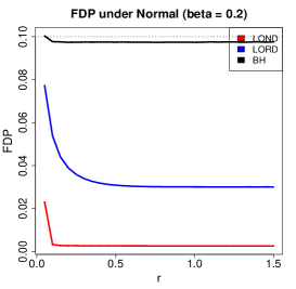
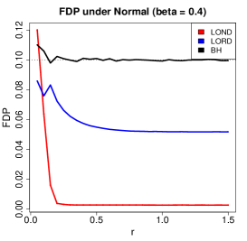
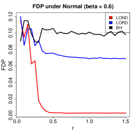
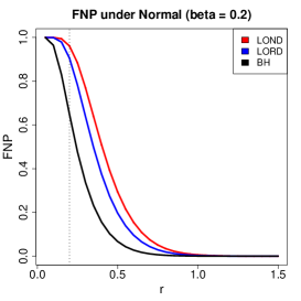
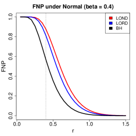
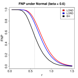
In this model $\Phi$ is the standard normal distribution. The simulation results are reported in Figure 1 and Figure 2. In Figure 1 we report the FDP. We see that LOND becomes more conservative than LORD as $r$ increases. In Figure 2 we report the FNP. We see that LOND is clearly less powerful than LORD in the regime $\beta=0.2$, but performs comparably to LORD in the regime $\beta=0.6$ . This is in line with the theory that LOND can at least achieve the line $r=\beta+(1-r^{1/\gamma})^{\gamma}$, which is getting closer to $r=\beta$ with increasing values of $\beta$. We notice that both LORD and LOND are clearly less powerful than BH in finite samples, even at $n=10^{9}$, even though our theory says that LORD achieves the same selection boundary as BH in the large-sample limit. Also, due to the limitation in choice of $\nu$ (here $\nu=1.05$), the selection boundary that LORD can achieve is $r=\nu\beta$ by theory, which explains why LORD lags behind BH. Finally, we remark the transition of LORD from high FNP to low FNP happens in the vicinity of the theoretical threshold ($r=\beta$).

Figure 1: Simulation results showing the FDP for the BH, LORD and LOND methods under the normal model in three distinct sparsity regimes. The black horizontal line delineates the desired FDR control level ($q=0.1$).

Figure 2: Simulation results showing the FNP for the BH, LORD and LOND methods under the normal model in three distinct sparsity regimes. The black vertical line delineates the theoretical threshold ($r=\beta$).

5.1.2 Double-exponential model

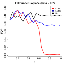
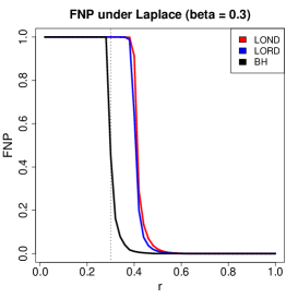
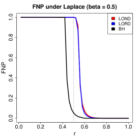
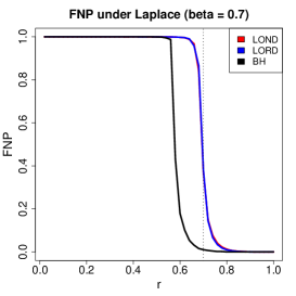
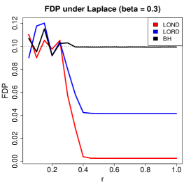
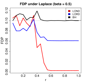
In this model $\Phi$ is the double-exponential distribution with variance 1. The simulation results are reported in Figure 3 (FDP) and Figure 4 (FNP). Here we observe that LOND becomes more conservative than LORD as $r$ increases in terms of FDP. The LOND and LORD perform more comparably than in the normal setting in terms of FNP, especially when $\beta$ is close to 1. This is again in line with our theoretical results. The BH method clearly outperforms the other two methods even though $n=10^{9}$. Due to the limitation in choice of $\nu$ (here $\nu=1.05$), the selection boundary that LORD can achieve is $r=\nu\beta$ by theory, which explains why LORD lags behind BH. The transition of three methods from FNP near 1 to FNP near 0 happens, again, in the vicinity of the theoretical threshold, but is much sharper here.

Figure 3: Simulation results showing the FDP for the BH, LORD and LOND methods under the double-exponential model in three distinct sparsity regimes. The black horizontal line delineates the desired FDR control level ($q=0.1$).

Figure 4: Simulation results showing the FNP for the BH, LORD and LOND methods under the double exponential model in three distinct sparsity regimes. The black vertical line delineates the theoretical threshold ($r=\beta$).

5.2 Varying sample size

In this second set of experiments we examine the effect of various sample sizes on the risk of the LORD and LOND procedures under the standard normal model and the double-exponential model (with variance 1).

5.2.1 FNR of LORD with a fixed level

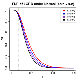
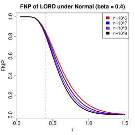
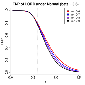
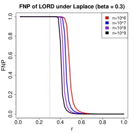
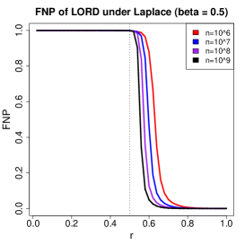
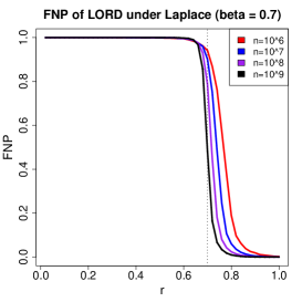
In this subsection, we present numerical experiments meant to illustrate the theoretical results we derived about asymptotic FNR of LORD. We fix $q=0.1$ , and choose a few values for the parameter $\beta$ so as to exhibit different sparsity levels, while the parameter $r$ takes values in a grid of spanning $[0,1.5]$. We plot the average FNP of LORD procedure with different $n\in\{10^{6},10^{7},10^{8},10^{9}\}$. The simulation results are reported in Figure 5 and Figure 6. Each situation is repeated 200 times. We observe that in the normal model when $r>\beta$, the FNP decreases as n is getting larger. In the double-exponential model, as $n$ increases, the FNP transition lines are getting closer the theoretical thresholds $r=\beta$, especially when $\beta=0.7$.

Figure 5: Simulation results showing the FNP for LORD under the normal model in three distinct sparsity regimes with different sample size. The black vertical line delineates the theoretical threshold ($r=\beta$).

Figure 6: Simulation results showing the FNP for LORD under the double exponential model in three distinct sparsity regimes with different sample size. The black vertical line delineates the theoretical threshold ($r=\beta$).

5.2.2 Varying level

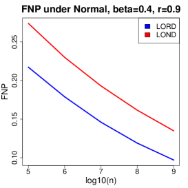
Here we explore the effect of letting the desired FDR control level $q$ tend to 0 as $n$ increases in accordance with (11). Specifically, we set it as $q=q_{n}=1/\log n$. We choose $n$ on a log scale, specifically, $n\in\{10^{5},10^{6},10^{7},10^{8},10^{9}\}$. Each time, we fix a value of $(\beta,r)$ such that $r>\beta$.

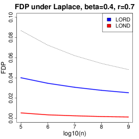
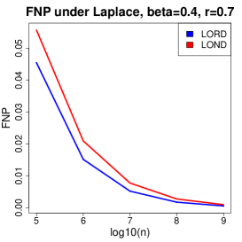
In the first setting, we set $(\beta,r)=(0.4,0.9)$ for normal model and $(\beta,r)=(0.4,0.7)$ for double-exponential model. The simulation results are reported in Figure 7 and Figure 8. We see that, in both models, the risks of the two procedures decrease to zero as the sample size gets larger. LORD clearly dominates LOND (in terms of FNP). Both methods have FDP much lower than the level $q_{n}$, and in particular, LOND is very conservative.

Figure 7: FDP and FNP for the LORD and LOND methods under the normal model with $(\beta,r)=(0.4,0.9)$ and varying sample size $n$. The black line delineates the desired FDR control level ($q=q_{n}$).

Figure 8: FDP and FNP for the LORD and LOND methods under the double-exponential model with $(\beta,r)=(0.4,0.7)$ and varying sample size $n$. The black line delineates the desired FDR control level ($q=q_{n}$).

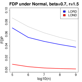
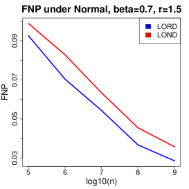
Figure 9: FDP and FNP for the LORD and LOND methods under the normal model with $(\beta,r)=(0.7,1.5)$ and varying sample size $n$. The black line delineates the desired FDR control level ($q=q_{n}$).

Figure 10: FDP and FNP for the LORD and LOND methods under the double-exponential model with $(\beta,r)=(0.7,0.9)$ and varying sample size $n$.

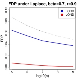
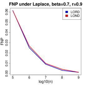
In the second setting, we set $(\beta,r)=(0.7,1.5)$ for normal model and $(\beta,r)=(0.7,0.9)$ for double-exponential model. The simulation results are reported in Figure 9 and Figure 10. In this sparser regime, we can see that although LORD still dominates, the difference in FNP between two methods is much smaller than that in dense regime, especially in the double-exponential model. Both methods have FDP lower than the level $q_{n}$, and in particular, LOND is very conservative.

6 Proofs

We prove our results in this section. Let $\Phi$ denote the CDF of null distribution. Without loss of generality, we assume throughout that $\Phi(0)=1/2$. Let $F(t)$ denote the CDF of the P-values under alternatives so that

$$F(t)=\Phi(\mu-\Phi^{-1}(1-t)),$$ (14)

where $\Phi^{-1}$ is the inverse function of $\Phi$. Let

$$G(t)=(1-\varepsilon)t+\varepsilon F(t),$$ (15)

which is the CDF of the P-values from the mixture model. Let $\bar{F}=1-F$, which is the survival function of the P-values under alternatives. Note that

$$\bar{F}(t)=1-F(t)=1-\Phi(\mu-\xi)=\bar{\Phi}(\mu-\xi),$$ (16)

where $\xi:=\Phi^{-1}(1-t)$, or equivalently, $t=\bar{\Phi}(\xi)$. Because $\Phi$ is as in Definition 1, when $\xi\to\infty$, we have

$$t=\bar{\Phi}(\xi)=\exp\Big{\{}-\frac{\xi^{\gamma}}{\gamma}(1+o(1))\Big{\}}\to 0,$$ (17)

which also implies, when $t\to 0$, that

$$\xi=\Phi^{-1}(1-t)\sim(\gamma\log(1/t))^{1/\gamma}.$$ (18)

6.1 Discovery times (LORD)

We apply LORD to the static setting under consideration. Denote $\tau_{l}$ as the time of $l$-th discovery (with $\tau_{0}=0$), and $\Delta_{l}=\tau_{l}-\tau_{l-1}$ as the time between the $(l-1)$-th and $l$-th discoveries. Assume a sequence satisfying (5) has been chosen. Given the update rule of (6), it can be seen that the inter-discovery times $\{\Delta_{l}:l\geq 1\}$ are IID.

To prove Theorem 1, we will use the following bound on the expected inter-discovery time.

Proposition 1.

Consider a static AGG mixture model with exponent $\gamma\geq 1$ parameterized as in (10). Assume that $\beta\in(0,1)$ and $r\geq 0$ are both fixed. Assume that $r>\beta$ and let $\nu>1$ be such that $\nu<r/\beta$. If we apply LORD with $(\lambda_{i})_{i=1}^{\infty}$ defined as $\lambda_{i}\propto i^{-\nu}$ with $\sum_{i=1}^{\infty}\lambda_{i}=q$,

$$\operatorname{\mathbb{E}}(\Delta_{l}\wedge n)\leq 2n^{\beta}+C,\quad\text{for all }l>0,$$ (19)

for some $C>0$ that does not depend on $n$. The same holds if we apply LORD with $(\lambda_{i})_{i=1}^{\infty}$ satisfying (12) and $\sum_{i=1}^{\infty}\lambda_{i}=q$.

We prove this result. Recall the definition of $G$ in (15) and note that $G\geq\varepsilon F$. By the update rule of LORD algorithm, for all $m\geq 1$ we have

$$\operatorname{\mathbb{P}}(\Delta_{l}>m) =\prod_{i=\tau_{l-1}+1}^{\tau_{l-1}+m}(1-G(\alpha_{i}))=\prod_{i=\tau_{l-1}+1}^{\tau_{l-1}+m}(1-G(\lambda_{i-\tau_{l-1}}))$$ (20)

$$=\prod_{i=1}^{m}(1-G(\lambda_{i}))\leq\exp\Big{\{}-\sum_{i=1}^{m}G(\lambda_{i})\Big{\}}\leq\exp\Big{\{}-\varepsilon\sum_{i=1}^{m}F(\lambda_{i})\Big{\}}.$$ (21)

Let $t^{*}$ be the value such that $\Phi^{-1}(1-t^{*})=\mu$, i.e., $t^{*}=\Phi(-\mu)=n^{-r+o(1)}$ by the fact that $\Phi$ satisfies Definition 1. Then, for $t\geq t^{*}$, we get

$$\Phi^{-1}(1-t)\leq\Phi^{-1}(1-t^{*})=\mu,$$ (22)

and then

$$F(t)=\Phi(\mu-\Phi^{-1}(1-t))\geq\Phi(\mu-\Phi^{-1}(1-t^{*}))=\Phi(\mu-\mu)=\Phi(0)=1/2,$$ (23)

so that if $\lambda_{i}=Li^{-\nu}\geq t^{*}$, i.e., $i\leq n_{1}:=\lfloor(L/t^{*})^{1/\nu}\rfloor=n^{r/\nu+o(1)}$, we have $F(\lambda_{i})\geq\Phi(0)=1/2$.

Remark 6.

If instead $(\lambda_{i})_{i=1}^{\infty}$ satisfies (12) then $i^{\nu}\lambda_{i}\to\infty$ as $i\to\infty$, so that exists a constant $L>0$ such that $\lambda_{i}\geq Li^{-\nu}$ for all $i$, and this is all that we need to proceed.

Thus, for $m\leq n_{1}$,

$$\sum_{i=1}^{m}F(\lambda_{i})\geq m/2,$$ (24)

and for $m>n_{1}$,

$$\sum_{i=1}^{m}F(\lambda_{i})\geq\sum_{i=1}^{n_{1}}F(\lambda_{i})\geq n_{1}/2.$$ (25)

Thus,

$$\operatorname{\mathbb{P}}(\Delta_{l}>m)\leq\exp\{-\varepsilon(m\wedge n_{1})/2\}.$$ (26)

Next we bound $\operatorname{\mathbb{E}}(\Delta_{l}\wedge n)$. Due to the fact that $\{\Delta_{l}\wedge n>m\}=\{\Delta_{l}>m\}$ for $1\leq m\leq n-1$, and $\{\Delta_{l}\wedge n>m\}=\emptyset$ if $m\geq n$, we have

$$\operatorname{\mathbb{E}}(\Delta_{l}\wedge n) =\sum_{m=0}^{\infty}\operatorname{\mathbb{P}}(\Delta_{l}\wedge n>m)$$ (27)

$$=\sum_{m=1}^{n-1}\operatorname{\mathbb{P}}(\Delta_{l}>m)+1$$ (28)

$$\leq\sum_{m=1}^{n-1}\exp\{-\varepsilon(m\wedge n_{1})/2\}+1.$$ (29)

We split the summation over $1\leq m\leq n_{1}$ and $n_{1}+1\leq m\leq n$ and derive the corresponding upper bound separately. For the first part,

$$\sum_{m=1}^{n_{1}}\exp\{-\varepsilon(m\wedge n_{1})/2\}=\sum_{m=1}^{n_{1}}\exp\{-\varepsilon m/2\}\leq\frac{1}{\exp\{\varepsilon/2\}-1}<\frac{2}{\varepsilon}=2n^{\beta}.$$ (30)

For the second part,

$$\sum_{m=n_{1}+1}^{n-1}\exp\{-\varepsilon(m\wedge n_{1})/2\}=\sum_{m=n_{1}+1}^{n-1}\exp\{-\varepsilon n_{1}/2\}\leq n\exp\{-\varepsilon n_{1}/2\}=o(1),$$ (31)

since $\varepsilon n_{1}=n^{r/\nu-\beta+o(1)}$ and $\frac{r}{\nu}>\beta$. Combining the above two bounds, we obtain

$$\operatorname{\mathbb{E}}(\Delta_{l}\wedge n)\leq 2n^{\beta}+o(1)+1.$$ (32)

This establishes Proposition 1.

6.2 Proof of Theorem 1

Note the number of false nulls is $m=|\mathscr{F}_{n}|=\varepsilon n\sim n^{1-\beta}$. The false non-discovery rate of LORD (denoted $\textsc{fnr}_{n}$) is as follows:

$$\textsc{fnr}_{n} =\operatorname{\mathbb{E}}\bigg{(}\frac{\sum_{i=1}^{n}\mathbb{I}\{i\notin\mathcal{H}_{0}(n):P_{i}\geq\alpha_{i}\}}{m}\bigg{)}$$ (33)

$$=\frac{\sum_{i=1}^{n}\operatorname{\mathbb{E}}[\operatorname{\mathbb{E}}(\mathbb{I}\{i\notin\mathcal{H}_{0}(n):P_{i}\geq\alpha_{i}\}\mid\alpha_{i})]}{m}$$ (34)

$$=\frac{\sum_{i=1}^{n}\operatorname{\mathbb{E}}[\operatorname{\mathbb{P}}(i\notin\mathcal{H}_{0}(n),P_{i}\geq\alpha_{i}\mid\alpha_{i})]}{m}$$ (35)

$$=\frac{\sum_{i=1}^{n}\operatorname{\mathbb{E}}[\varepsilon\bar{F}(\alpha_{i})]}{\varepsilon n}$$ (36)

$$=\frac{\sum_{i=1}^{n}\operatorname{\mathbb{E}}[\bar{F}(\alpha_{i})]}{n}.$$ (37)

So it suffices to bound the RHS of the equation.

Let $D(n)$ be the number of discoveries in first $n$ hypotheses $\mathcal{H}(n)$ by applying LORD with the sequence $(\lambda_{i})$. Let $\tilde{\Delta}_{l}=\Delta_{l}=\tau_{l}-\tau_{l-1}$, for $1\leq l\leq D(n)$, and $\tilde{\Delta}_{D(n)+1}=n-\tau_{D(n)}$. Due to the fact that $0\leq\tilde{\Delta}_{l}\leq(\Delta_{l}\wedge n)$, for $1\leq l\leq D(n)+1$, we have for any fixed $\delta>0$ ,

$$\operatorname{\mathbb{P}}(\tilde{\Delta}_{l}\geq\frac{\operatorname{\mathbb{E}}(\Delta_{l}\wedge n)}{\delta})\leq\frac{\operatorname{\mathbb{E}}(\tilde{\Delta}_{l})}{\operatorname{\mathbb{E}}(\Delta_{l}\wedge n)}\cdot\delta\leq\delta,\quad\text{for }1\leq l\leq D(n)+1,$$ (38)

by Markov Inequality. Note that $(\Delta_{l}\wedge n)$’s are IID. We define $M_{n}:=\left\lceil\operatorname{\mathbb{E}}(\Delta)/\delta\right\rceil$, where $\Delta\overset{d}{=}\Delta_{l}\wedge n$ for all $l>0$.

For any $i\in\mathcal{H}(n)$, there exists only one $j=j(i)\in\{1,2,\dots,D(n)+1\}$ such that $i\in(\tau_{j-1},\tau_{j}\wedge n]$, and

$$\operatorname{\mathbb{E}}\big{[}\bar{F}(\alpha_{i})\big{]} =\operatorname{\mathbb{E}}\big{[}\bar{F}(\alpha_{i})\cdot\mathbb{I}\{\tilde{\Delta}_{j(i)}\geq M_{n}\}\big{]}+\operatorname{\mathbb{E}}\big{[}\bar{F}(\alpha_{i})\cdot\mathbb{I}\{\tilde{\Delta}_{j(i)}<M_{n}\}\big{]}$$ (39)

$$\leq\delta+\operatorname{\mathbb{E}}\big{[}\bar{F}(\alpha_{i})\cdot\mathbb{I}\{\tilde{\Delta}_{j(i)}<M_{n}\}\big{]},$$ (40)

so that

$$\sum_{i=1}^{n}\operatorname{\mathbb{E}}\big{[}\bar{F}(\alpha_{i})\big{]}\leq n\delta+\operatorname{\mathbb{E}}\bigg{[}\sum_{i=1}^{n}\bar{F}(\alpha_{i})\cdot\mathbb{I}\{\tilde{\Delta}_{j(i)}<M_{n}\}\bigg{]}.$$ (41)

By Proposition 1, there is $C>0$ not depending on $n$ such that

$$\operatorname{\mathbb{E}}(\Delta)\leq 2n^{\beta}+C,\quad\text{for all }l>0.$$ (42)

And thus, there is some $L^{\prime}>0$ (constant in $n$) such that, for $1\leq i\leq M_{n}$,

$$\lambda_{i}=Li^{-\nu}\geq L\cdot(M_{n})^{-\nu}=L\cdot\left\lceil\operatorname{\mathbb{E}}(\Delta)/\delta\right\rceil^{-\nu}\geq L\cdot\left\lceil(2n^{\beta}+C)/\delta\right\rceil^{-\nu}\geq L^{\prime}n^{-\beta\nu}.$$ (43)

Remark 7.

If instead $(\lambda_{i})_{i=1}^{\infty}$ satisfies (12) then $i^{\nu}\lambda_{i}\to\infty$ as $i\to\infty$, so that exists a constant $L>0$ such that $\lambda_{i}\geq Li^{-\nu}$ for all $i$, and this is all that we need to proceed.

Since $\bar{F}$ is a decreasing function, the second term in RHS of (41) can be bounded as

$$\operatorname{\mathbb{E}}\bigg{[}\sum_{i=1}^{n}\bar{F}(\alpha_{i})\cdot\mathbb{I}\{\tilde{\Delta}_{j(i)}<M_{n}\}\bigg{]} =\operatorname{\mathbb{E}}\bigg{[}\sum_{j=1}^{D(n)+1}\sum_{i=\tau_{j-1}+1}^{\tau_{j}\wedge n}\bar{F}(\alpha_{i})\cdot\mathbb{I}\{\tilde{\Delta}_{j}<M_{n}\}\bigg{]}$$ (44)

$$=\operatorname{\mathbb{E}}\bigg{[}\sum_{j=1}^{D(n)+1}\sum_{i=1}^{\tilde{\Delta}_{j}}\bar{F}(\lambda_{i})\cdot\mathbb{I}\{\tilde{\Delta}_{j}<M_{n}\}\bigg{]}$$ (45)

$$\leq\operatorname{\mathbb{E}}\bigg{[}\sum_{j=1}^{D(n)+1}\sum_{i=1}^{\tilde{\Delta}_{j}}\bar{F}(L^{\prime}n^{-\beta\nu})\cdot\mathbb{I}\{\tilde{\Delta}_{j}<M_{n}\}\bigg{]}$$ (46)

$$\leq\operatorname{\mathbb{E}}\bigg{[}\sum_{i=1}^{n}\bar{F}(L^{\prime}n^{-\beta\nu})\bigg{]}\leq n\cdot\bar{F}(L^{\prime}n^{-\beta\nu}).$$ (47)

Combining these bounds, we obtain

$$\textsc{fnr}_{n}(\mathscr{R})=\frac{\sum_{i=1}^{n}\operatorname{\mathbb{E}}[\bar{F}(\alpha_{i})]}{n}\leq\delta+\bar{F}(L^{\prime}n^{-\beta\nu}).$$ (48)

Since $L^{\prime}n^{-\beta\nu}\to 0$ as $n\to\infty$, by equation (18) we have

$$\xi_{n}:=\Phi^{-1}(1-L^{\prime}n^{-\beta\nu})=(\gamma\beta\nu\log n)^{1/\gamma}(1+o(1)),$$ (49)

so that

$$\mu-\xi_{n} =(\gamma r\log n)^{1/\gamma}-(\gamma\beta\nu\log n)^{1/\gamma}(1+o(1))$$ (50)

$$\sim(r^{1/\gamma}-(\beta\nu)^{1/\gamma})(\gamma\log n)^{1/\gamma}\to\infty,\quad\text{as }n\to\infty,$$ (51)

since $r>\beta\nu$. Therefore, $\bar{F}(L^{\prime}n^{-\beta\nu})=\bar{\Phi}(\mu-\xi_{n})\to 0$ as $n\to\infty$. Hence,

$$\limsup_{n\to\infty}\textsc{fnr}_{n}\leq\delta.$$ (52)

This being true for any $\delta>0$, necessarily, $\textsc{fnr}_{n}\to 0$ as $n\to\infty$. This establishes Theorem 1.

6.3 Discovery times (LOND)

We apply LOND to the static setting under consideration. Denote $\tau_{l}$ as the time of $l$-th discovery (with $\tau_{0}=0$), and $\Delta_{l}=\tau_{l}-\tau_{l-1}$ as the time between the $(l-1)$-th and $l$-th discoveries. Assume a sequence satisfying (5) has been chosen. Given the update rule of (8), it can be seen that the inter-discovery times $\{\Delta_{l}:l\geq 1\}$ are i.i.d..

To prove Theorem 2, we will use the following bound on the expected discovery times.

Proposition 2.

Consider a static AGG mixture model with exponent $\gamma\geq 1$ parameterized as in (10). Assume that $\beta\in(0,1)$ and $r\in[0,1]$ are both fixed. For any $\nu>1$, if we apply LOND with $(\lambda_{i})_{i=1}^{\infty}$ defined as $\lambda_{i}\propto i^{-\nu}$ with $\sum_{i=1}^{\infty}\lambda_{i}=q$,

$$\operatorname{\mathbb{E}}(\tau_{l}\wedge n)\leq l\cdot n^{\beta+(\nu^{1/\gamma}-r^{1/\gamma})^{\gamma}+b_{n}},\quad\text{for all }l>0,$$ (53)

where $b_{n}\to 0$ as $n\to\infty$.

We now prove this result. By the update rule of LOND algorithm, for all $l\geq 0$, and all $m\geq\tau_{l}+1$, we have

$$\operatorname{\mathbb{P}}(\tau_{l+1}>m\mid\tau_{l})=\prod_{i=\tau_{l}+1}^{m}(1-G((l+1)\lambda_{i}))\leq\exp\{-\sum_{i=\tau_{l}+1}^{m}G((l+1)\lambda_{i})\}.$$ (54)

Note $\tau_{l}$ is the time of $l$-th discovery (with $\tau_{0}=0$) by LOND. Let $\tilde{\tau}_{l}=\tau_{l}\wedge n$. If $\tilde{\tau}_{l}=n$, we have $\operatorname{\mathbb{E}}(\tilde{\tau}_{l+1}\mid\tilde{\tau}_{l})=n=\tilde{\tau}_{l}$. Otherwise, if $\tilde{\tau}_{l}=\tau_{l}<n$,

$$\operatorname{\mathbb{E}}(\tilde{\tau}_{l+1}\mid\tilde{\tau}_{l}) =\tau_{l}+1+\sum_{m=\tau_{l}+1}^{\infty}\operatorname{\mathbb{P}}(\tau_{l+1}\wedge n>m\mid\tau_{l})$$ (55)

$$=\tau_{l}+1+\sum_{m=\tau_{l}+1}^{n-1}\operatorname{\mathbb{P}}(\tau_{l+1}>m\mid\tau_{l})$$ (56)

$$\leq\tau_{l}+1+\sum_{m=\tau_{l}+1}^{n}\exp\{-\sum_{i=\tau_{l}+1}^{m}G((l+1)\lambda_{i})\}$$ (57)

$$=\tilde{\tau}_{l}+1+\sum_{m=\tilde{\tau}_{l}+1}^{n}\exp\{-\sum_{i=\tilde{\tau}_{l}+1}^{m}G((l+1)\lambda_{i})\}.$$ (58)

Next we bound $\operatorname{\mathbb{E}}(\tilde{\tau}_{l+1}\mid\tilde{\tau}_{l})$. Let $t^{*}$ be the value such that $\Phi^{-1}(1-t^{*})=\mu$, i.e., $t^{*}=\Phi(-\mu)=n^{-r+o(1)}$ by the fact that $\Phi$ satisfies Definition 1. Then, for $t\geq t^{*}$, we get

$$\Phi^{-1}(1-t)\leq\Phi^{-1}(1-t^{*})=\mu,$$ (59)

and,

$$F(t)=\Phi(\mu-\Phi^{-1}(1-t))\geq\Phi(\mu-\Phi^{-1}(1-t^{*}))=\Phi(\mu-\mu)=\Phi(0)=1/2,$$ (60)

so that if $(l+1)\lambda_{i}=(l+1)Li^{-\nu}\geq t^{*}$, i.e., $i\leq n_{1}:=\lfloor((l+1)L/t^{*})^{1/\nu}\rfloor=n^{r/\nu+o(1)}$, we have $F((l+1)\lambda_{i})\geq\Phi(0)=1/2$.

We consider the following cases.

Case 1: $\tilde{\tau}_{l}<n_{1}<n$.

In this case, for $\tilde{\tau}_{l}+1\leq m\leq n_{1}$,

$$\sum_{i=\tilde{\tau}_{l}+1}^{m}G((l+1)\lambda_{i})\geq\sum_{i=\tilde{\tau}_{l}+1}^{m}\varepsilon F((l+1)\lambda_{i})\geq\varepsilon\cdot(m-\tilde{\tau}_{l})/2,$$ (61)

and for $m>n_{1}$,

$$\sum_{i=\tilde{\tau}_{l}+1}^{m}G((l+1)\lambda_{i})\geq\sum_{i=\tilde{\tau}_{l}+1}^{m}\varepsilon F((l+1)\lambda_{i})\geq\sum_{i=\tilde{\tau}_{l}+1}^{m}\varepsilon F((l+1)\lambda_{m})=(m-\tilde{\tau}_{l})\varepsilon F((l+1)\lambda_{m}),$$ (62)

since $F(x)$ is non-decreasing.

We split the summation in (58) over $\tau_{l}+1\leq m\leq n_{1}$ and $n_{1}+1\leq m\leq n$ and derive the corresponding upper bound separately. For the first part,

$$\sum_{m=\tilde{\tau}_{l}+1}^{n_{1}}\exp\{-\sum_{i=\tilde{\tau}_{l}+1}^{m}G((l+1)\lambda_{i})\} \leq\sum_{m=\tilde{\tau}_{l}+1}^{n_{1}}\exp\{-\varepsilon(m-\tilde{\tau}_{l})/2\}=\sum_{m=1}^{n_{1}-\tilde{\tau}_{l}}\exp\{-\varepsilon m/2\}$$ (63)

$$\leq\frac{1}{\exp\{\varepsilon/2\}-1}<\frac{2}{\varepsilon}=2n^{\beta}.$$ (64)

For the second part,

$$\sum_{m=n_{1}+1}^{n}\exp\Big{\{}-\sum_{i=\tilde{\tau}_{l}+1}^{m}G((l+1)\lambda_{i})\Big{\}} \leq\sum_{m=n_{1}+1}^{n}\exp\{-(m-\tilde{\tau}_{l})\varepsilon F((l+1)\lambda_{m})\}$$ (65)

$$\leq\sum_{m=n_{1}+1}^{n}\exp\{-(m-n_{1})\varepsilon F((l+1)\lambda_{n})\}$$ (66)

$$\leq\sum_{m=1}^{n-n_{1}}\exp\{-m\varepsilon F((l+1)\lambda_{n})\}$$ (67)

$$\leq\frac{1}{\exp\{\varepsilon F((l+1)\lambda_{n})\}-1}$$ (68)

$$<\frac{1}{\varepsilon F((l+1)\lambda_{n})}\leq\frac{1}{\varepsilon F(\lambda_{n})}.$$ (69)

Case 2: $n_{1}\leq\tilde{\tau}_{l}<n$.

For this case, we don’t need to split the summation, since

$$\sum_{m=\tilde{\tau}_{l}+1}^{n}\exp\{-\sum_{i=\tilde{\tau}_{l}+1}^{m}G((l+1)\lambda_{i})\} \leq\sum_{m=\tilde{\tau}_{l}+1}^{n}\exp\{-(m-\tilde{\tau}_{l})\varepsilon F((l+1)\lambda_{m})\}$$ (70)

$$\leq\sum_{m=1}^{n-\tilde{\tau}_{l}}\exp\{-m\varepsilon F((l+1)\lambda_{n})\}$$ (71)

$$<\frac{1}{\varepsilon F((l+1)\lambda_{n})}\leq\frac{1}{\varepsilon F(\lambda_{n})}.$$ (72)

Case 3: $n_{1}\geq n$.

Since $\tilde{\tau}_{l}<n\leq n_{1}$, we have that

$$\sum_{m=\tilde{\tau}_{l}+1}^{n}\exp\{-\sum_{i=\tilde{\tau}_{l}+1}^{m}G((l+1)\lambda_{i})\} \leq\sum_{m=\tilde{\tau}_{l}+1}^{n}\exp\{-(m-\tilde{\tau}_{l})\varepsilon/2\}$$ (73)

$$\leq\sum_{m=1}^{n-\tilde{\tau}_{l}}\exp\{-m\varepsilon/2\}<\frac{2}{\varepsilon}=2n^{\beta}.$$ (74)

Combining all the cases, we obtain

$$\operatorname{\mathbb{E}}(\tilde{\tau}_{l+1}\mid\tilde{\tau}_{l})\leq\tilde{\tau}_{l}+1+\frac{2}{\varepsilon}+\frac{1}{\varepsilon F(\lambda_{n})},$$ (75)

where $F(\lambda_{n})=\bar{\Phi}(\xi_{n}-\mu)$, and $\xi_{n}:=\Phi^{-1}(1-\lambda_{n})$. Since $\lambda_{n}=Ln^{-\nu}\to 0$ as $n\to 0$, by equation (18), we have $\xi_{n}\sim(\gamma\nu\log n)^{1/\gamma}$, so that

$$\xi_{n}-\mu =(\gamma\nu\log n)^{1/\gamma}(1+o(1))-(\gamma r\log n)^{1/\gamma}$$ (76)

$$\sim(\nu^{1/\gamma}-r^{1/\gamma})(\gamma\log n)^{1/\gamma}\to\infty,\quad\text{as }n\to\infty,$$ (77)

by the fact that $\nu>1\geq r$. By Definition 1,

$$F(\lambda_{n})=\bar{\Phi}(\xi_{n}-\mu)=\exp\Big{\{}-\frac{(\xi_{n}-\mu)^{\gamma}}{\gamma}(1+o(1))\Big{\}}=n^{-(\nu^{1/\gamma}-r^{1/\gamma})^{\gamma}+o(1)}.$$ (78)

Thus, when $n$ is large enough,

$$\operatorname{\mathbb{E}}(\tilde{\tau}_{l+1}\mid\tilde{\tau}_{l})\leq\tilde{\tau}_{l}+1+\frac{2}{\varepsilon}+\frac{1}{\varepsilon F(\lambda_{n})}\leq\tilde{\tau}_{l}+n^{\beta+(\nu^{1/\gamma}-r^{1/\gamma})^{\gamma}+o(1)},\quad\text{for all }l>0,$$ (79)

where the $o(1)$ is uniform in $l$, and this further implies that

$$\operatorname{\mathbb{E}}(\tilde{\tau}_{l+1})=\operatorname{\mathbb{E}}[\operatorname{\mathbb{E}}(\tilde{\tau}_{l+1}\mid\tilde{\tau}_{l})]\leq\operatorname{\mathbb{E}}(\tilde{\tau}_{l})+n^{\beta+(\nu^{1/\gamma}-r^{1/\gamma})^{\gamma}+o(1)},\quad\text{for all }l>0,$$ (80)

so that

$$\operatorname{\mathbb{E}}(\tau_{l}\wedge n)\leq l\cdot n^{\beta+(\nu^{1/\gamma}-r^{1/\gamma})^{\gamma}+o(1)},\quad\text{for all }l>0.$$ (81)

6.4 Proof of Theorem 2

It suffices to consider the case where $r\in[0,1]$ since the observations from $\mathbb{H}_{0}$ almost never get substantially larger than $(\gamma\log n)^{1/\gamma}$. For $r\in[0,1]$, if $r-(1-r^{1/\gamma})^{\gamma}>\beta$, we can choose $\nu>1$ close to 1 and $\eta>0$ close to 0 such that $r>\rho:=\beta+(\nu^{1/\gamma}-r^{1/\gamma})^{\gamma}+\nu-1+\eta$. By Proposition 2, when $n$ is large enough,

$$\operatorname{\mathbb{E}}(\tau_{l}\wedge n)\leq l\cdot n^{\beta+(\nu^{1/\gamma}-r^{1/\gamma})^{\gamma}+\eta},\quad\text{for all }l>0.$$ (82)

Fix $\delta>0$ and let $n_{2}:=\lceil n^{\beta+(\nu^{1/\gamma}-r^{1/\gamma})^{\gamma}+\eta}/\delta\rceil$. Note $n_{2}=o(n)$, since $1\geq r>\beta+(\nu^{1/\gamma}-r^{1/\gamma})^{\gamma}+\eta$.

For $n_{2}\leq i\leq n$, let $\zeta_{i}:=i\,\delta\,n^{-\beta-(\nu^{1/\gamma}-r^{1/\gamma})^{\gamma}-\eta}$, we get

$$\operatorname{\mathbb{P}}(D(i)<\zeta_{i}) =\operatorname{\mathbb{P}}(\tau_{\lceil\zeta_{i}\rceil}>i)\leq\operatorname{\mathbb{P}}(\tau_{\lceil\zeta_{i}\rceil}\geq i)=\operatorname{\mathbb{P}}(\tau_{\lceil\zeta_{i}\rceil}\wedge n\geq i)$$ (83)

$$\leq\frac{\operatorname{\mathbb{E}}(\tau_{\lceil\zeta_{i}\rceil}\wedge n)}{i}\leq\frac{\lceil\zeta_{i}\rceil\cdot n^{\beta+(\nu^{1/\gamma}-r^{1/\gamma})^{\gamma}+\eta}}{i}$$ (84)

$$<\frac{(\zeta_{i}+1)\cdot n^{\beta+(\nu^{1/\gamma}-r^{1/\gamma})^{\gamma}+\eta}}{i}$$ (85)

$$=\delta+\frac{n^{\beta+(\nu^{1/\gamma}-r^{1/\gamma})^{\gamma}+\eta}}{i}<2\delta.$$ (86)

By Rule (8) defining the LOND algorithm,

$$\operatorname{\mathbb{E}}[\bar{F}(\alpha_{i})]=\operatorname{\mathbb{E}}[\bar{F}(\lambda_{i}(D(i-1)+1))]\leq\operatorname{\mathbb{E}}[\bar{F}(\lambda_{i}D(i))],$$ (87)

due to the fact that $D(i-1)+1\geq D(i)$ and that $\bar{F}(x)$ is a non-increasing function, so that LOND’s false non-discovery rate (denoted $\textsc{fnr}_{n}$) is bounded as follows

$$\textsc{fnr}_{n}=\frac{1}{n}\sum_{i=1}^{n}\operatorname{\mathbb{E}}[\bar{F}(\alpha_{i})]\leq\frac{1}{n}\sum_{i=1}^{n}\operatorname{\mathbb{E}}[\bar{F}(\lambda_{i}D(i))].$$ (88)

For $1\leq i\leq n_{2}$,

$$\frac{1}{n}\sum_{i=1}^{n_{2}}\operatorname{\mathbb{E}}[\bar{F}(\lambda_{i}D(i))]\leq\frac{n_{2}}{n}.$$ (89)

And for $n_{2}+1\leq i\leq n$,

$$\operatorname{\mathbb{E}}[\bar{F}(\lambda_{i}D(i))] =\operatorname{\mathbb{E}}[\bar{F}(\lambda_{i}D(i))\cdot\mathbb{I}\{D(i)<\zeta_{i}\}]+\operatorname{\mathbb{E}}[\bar{F}(\lambda_{i}D(i))\cdot\mathbb{I}\{D(i)\geq\zeta_{i}\}]$$ (90)

$$\leq 2\delta+\bar{F}(\lambda_{i}\zeta_{i}),$$ (91)

and since $\nu>1$, we have

$$\lambda_{i}\zeta_{i}=L\delta\cdot i^{1-\nu}\cdot n^{-\beta-(\nu^{1/\gamma}-r^{1/\gamma})^{\gamma}-\eta}\geq L\delta\cdot n^{1-\nu}\cdot n^{-\beta-(\nu^{1/\gamma}-r^{1/\gamma})^{\gamma}-\eta}=\lambda_{n}\zeta_{n},$$ (92)

which implies that,

$$\frac{1}{n}\sum_{i=1}^{n}\operatorname{\mathbb{E}}[\bar{F}(\lambda_{i}D(i))]\leq\frac{n_{2}}{n}+\frac{n-n_{2}}{n}(2\delta+\bar{F}(\lambda_{n}\zeta_{n}))\leq 2\delta+\bar{F}(\lambda_{n}\zeta_{n})+o(1).$$ (93)

Since $\lambda_{n}\zeta_{n}=L\delta n^{-\rho}\to 0$ as $n\to\infty$, by equation (18)

$$\xi_{n}:=\Phi^{-1}(1-\lambda_{n}\zeta_{n})=(\gamma\rho\log n)^{1/\gamma}(1+o(1)),$$ (94)

then

$$\mu-\xi_{n} =(\gamma r\log n)^{1/\gamma}-(\gamma\rho\log n)^{1/\gamma}(1+o(1))$$ (95)

$$\sim(r^{1/\gamma}-\rho^{1/\gamma})(\gamma\log n)^{1/\gamma}\to\infty,\quad\text{as }n\to\infty,$$ (96)

since $r>\rho$. Therefore, $\bar{F}(\lambda_{n}\zeta_{n})=\bar{\Phi}(\mu-\xi_{n})\to 0$ as $n\to\infty$. Hence,

$$\limsup_{n\to\infty}\textsc{fnr}_{n}\leq 2\delta.$$ (97)

This being true for any $\delta>0$, necessarily, $\textsc{fnr}_{n}\to 0$ as $n\to\infty$.

7 Acknowledgement

We would like to thank Jiaqi Gu from Department of Computer Science, University of California, Los Angeles, for his help with the large-sample size numerical experiments in Section 5.

References

• Aharoni and Rosset (2014) Aharoni, E. and S. Rosset (2014). Generalized α𝛼\alpha-investing: definitions, optimality results and application to public databases. Journal of the Royal Statistical Society: Series B (Statistical Methodology) 76(4), 771–794.
• Arias-Castro and Chen (2016) Arias-Castro, E. and S. Chen (2016). Distribution-free multiple testing. arXiv preprint arXiv:1604.07520.
• Bartroff (2014) Bartroff, J. (2014). Multiple hypothesis tests controlling generalized error rates for sequential data. arXiv preprint arXiv:1406.5933.
• Bartroff and Song (2013) Bartroff, J. and J. Song (2013). Sequential tests of multiple hypotheses controlling false discovery and nondiscovery rates. arXiv preprint arXiv:1311.3350.
• Bartroff and Song (2014) Bartroff, J. and J. Song (2014). Sequential tests of multiple hypotheses controlling type i and ii familywise error rates. Journal of statistical planning and inference 153, 100–114.
• Benjamini and Hochberg (1995) Benjamini, Y. and Y. Hochberg (1995). Controlling the false discovery rate: A practical and powerful approach to multiple testing. Journal of the Royal Statistical Society. Series B (Methodological) 57(1), 289–300.
• Bogdan et al. (2011) Bogdan, M., A. Chakrabarti, F. Frommlet, and J. K. Ghosh (2011). Asymptotic bayes-optimality under sparsity of some multiple testing procedures. The Annals of Statistics, 1551–1579.
• Butucea et al. (2015) Butucea, C., N. A. Stepanova, and A. B. Tsybakov (2015). Variable selection with hamming loss. arXiv preprint arXiv:1512.01832.
• Dickhaus (2014) Dickhaus, T. (2014). Simultaneous statistical inference. Springer.
• Donoho and Jin (2004) Donoho, D. and J. Jin (2004). Higher criticism for detecting sparse heterogeneous mixtures. The Annals of Statistics 32(3), 962–994.
• Dudoit and van der Laan (2007) Dudoit, S. and M. J. van der Laan (2007). Multiple testing procedures with applications to genomics. Springer Science & Business Media.
• Fithian et al. (2014) Fithian, W., D. Sun, and J. Taylor (2014). Optimal inference after model selection. arXiv preprint arXiv:1410.2597.
• Fithian et al. (2015) Fithian, W., J. Taylor, R. Tibshirani, and R. Tibshirani (2015). Selective sequential model selection. arXiv preprint arXiv:1512.02565.
• Foster and Stine (2008) Foster, D. P. and R. A. Stine (2008). α𝛼\alpha-investing: a procedure for sequential control of expected false discoveries. Journal of the Royal Statistical Society: Series B (Statistical Methodology) 70(2), 429–444.
• Foygel-Barber and Candès (2015) Foygel-Barber, R. and E. J. Candès (2015). Controlling the false discovery rate via knockoffs. The Annals of Statistics 43(5), 2055–2085.
• Genovese and Wasserman (2002) Genovese, C. and L. Wasserman (2002). Operating characteristics and extensions of the false discovery rate procedure. Journal of the Royal Statistical Society: Series B (Statistical Methodology) 64(3), 499–517.
• G’Sell et al. (2016) G’Sell, M. G., S. Wager, A. Chouldechova, and R. Tibshirani (2016). Sequential selection procedures and false discovery rate control. Journal of the Royal Statistical Society: Series B (Statistical Methodology) 78(2), 423–444.
• Ingster (1997) Ingster, Y. I. (1997). Some problems of hypothesis testing leading to infinitely divisible distributions. Mathematical Methods of Statistics 6(1), 47–69.
• Ingster and Suslina (2003) Ingster, Y. I. and I. A. Suslina (2003). Nonparametric goodness-of-fit testing under Gaussian models, Volume 169 of Lecture Notes in Statistics. New York: Springer-Verlag.
• Javanmard and Montanari (2015) Javanmard, A. and A. Montanari (2015). On online control of false discovery rate. arXiv preprint arXiv:1502.06197.
• Javanmard and Montanari (2016) Javanmard, A. and A. Montanari (2016). Online rules for control of false discovery rate and false discovery exceedance. arXiv preprint arXiv:1603.09000.
• Ji et al. (2012) Ji, P., J. Jin, et al. (2012). Ups delivers optimal phase diagram in high-dimensional variable selection. The Annals of Statistics 40(1), 73–103.
• Jin and Ke (2014) Jin, J. and T. Ke (2014). Rare and weak effects in large-scale inference: methods and phase diagrams. arXiv preprint arXiv:1410.4578.
• Lei and Fithian (2016) Lei, L. and W. Fithian (2016). Power of ordered hypothesis testing. arXiv preprint arXiv:1606.01969.
• Li and Barber (2016) Li, A. and R. F. Barber (2016). Accumulation tests for fdr control in ordered hypothesis testing. Journal of the American Statistical Association (just-accepted), 1–38.
• Lockhart et al. (2014) Lockhart, R., J. Taylor, R. J. Tibshirani, and R. Tibshirani (2014). A significance test for the lasso. Annals of statistics 42(2), 413.
• Meinshausen et al. (2011) Meinshausen, N., M. H. Maathuis, P. Bühlmann, et al. (2011). Asymptotic optimality of the westfall–young permutation procedure for multiple testing under dependence. The Annals of Statistics 39(6), 3369–3391.
• Neuvial and Roquain (2012) Neuvial, P. and E. Roquain (2012). On false discovery rate thresholding for classification under sparsity. The Annals of Statistics 40(5), 2572–2600.
• Roquain (2011) Roquain, E. (2011). Type i error rate control in multiple testing: a survey with proofs. Journal de la Société Française de Statistique 152(2), 3–38.
• Storey (2007) Storey, J. D. (2007). The optimal discovery procedure: a new approach to simultaneous significance testing. Journal of the Royal Statistical Society: Series B (Statistical Methodology) 69(3), 347–368.
• Sun and Cai (2007) Sun, W. and T. T. Cai (2007). Oracle and adaptive compound decision rules for false discovery rate control. Journal of the American Statistical Association 102(479), 901–912.