Open-flavor charmed/bottom $sq\bar{q}\bar{Q}$ and $qq\bar{q}\bar{Q}$ tetraquark states

Abstract

We provide comprehensive investigations for the mass spectrum of exotic open-flavor charmed/bottom $sq\bar{q}\bar{c}$, $qq\bar{q}\bar{c}$, $sq\bar{q}\bar{b}$, $qq\bar{q}\bar{b}$ tetraquark states with various spin-parity assignments $J^{P}=0^{+},1^{+},2^{+}$ and $0^{-},1^{-}$ in the framework of QCD sum rules. In the diquark configuration, we construct the diquark-antidiquark interpolating tetraquark currents using the color-antisymmetric scalar and axial-vector diquark fields. The stable mass sum rules are established in reasonable parameter working ranges, which are used to give reliable mass predictions for these tetraquark states. We obtain the mass spectra for the open-flavor charmed/bottom $sq\bar{q}\bar{c}$, $qq\bar{q}\bar{c}$, $sq\bar{q}\bar{b}$, $qq\bar{q}\bar{b}$ tetraquark states with various spin-parity quantum numbers. In addition, we suggest searching for exotic doubly-charged tetraquarks, such as $[sd][\bar{u}\bar{c}]\to D_{s}^{(\ast)-}\pi^{-}$ in future experiments at facilities such as BESIII, BelleII, PANDA, LHCb and CMS, etc.

I Introduction

During the past 14 years, there are many unexpected hadrons observed experimentally, such as the XYZ states Patrignani et al. (2016) and hidden-charm pentaquarks Aaij et al. (2015), etc. These resonances cannot be interpreted as conventional quark-antiquark mesons or three-quark baryons in the conventional quark model Klempt and Zaitsev (2007). They are exotic hadron candidates, whose significant experimental and theoretical progress have been reviewed in Refs. Chen et al. (2016a); Esposito et al. (2015); Olsen (2015); Lebed et al. (2016).

Very recently, the D0 Collaboration reported the evidence for the narrow structure $X(5568)$ in the $B_{s}^{0}\pi^{\pm}$ invariant mass spectrum with 5.1$\sigma$ significance Abazov et al. (2016). Its mass and decay width were measured to be $m_{X(5568)}=5567.8\pm 2.9(\rm stat)^{+0.9}_{-1.9}(\rm syst){\rm~{}MeV}$ and $\Gamma_{X(5568)}=21.9\pm 6.4(\rm stat)^{+5.0}_{-2.5}(\rm syst){\rm~{}MeV}$, and its spin-parity quantum number was determined to be either $J^{P}=0^{+}$ or $1^{+}$. Later, the LHCb and CMS collaborations also performed their analyses of the $pp$ collision data at energies $\sqrt{s}=7$ TeV and 8 TeV to search for the $X(5568)$ state Aaij et al. (2016); Collaboration (2016), but they did not find any unexpected structure in the $B_{s}^{0}\pi^{\pm}$ invariant mass distribution. However, the D0 Collaboration themselves confirmed the $X(5568)$ meson in the $B_{s}^{0}\pi^{\pm}$ invariant mass distribution with another channel $B_{s}^{0}\to D_{s}\mu\nu$ at the same mass and at the expected width and rate Collaboration (2016).

Reported in the $B_{s}^{0}\pi^{\pm}$ final states, the $X(5568)$ meson, if it exists, could be a bottom-strange $su\bar{d}\bar{b}$ (or $sd\bar{u}\bar{b}$) tetraquark state with valence quarks of four different flavors. To date, the $X(5568)$ resonance has trigged many theoretical studies, including the diquark-antidiquark tetraquark state Chen et al. (2016b); Agaev et al. (2016a); Zanetti et al. (2016); Wang (2016a, b); Wang and Zhu (2016); Tang and Qiao (2016); Agaev et al. (2016b); Dias et al. (2016); Albuquerque et al. (2016); Liu et al. (2016); Stancu (2016); Ali et al. (2016); He and Ko (2016); Burns and Swanson (2016); Guo et al. (2016); Lü and Dong (2016); Goerke et al. (2016); Agamaliev et al. (2016), hadron molecule Agaev et al. (2016c); Kang and Oller (2016); Chen and Ping (2016); Albaladejo et al. (2016); Lang et al. (2016); Chen and Liu (2016); Lu et al. (2016); Sun et al. (2016), non-resonant schemes Liu and Li (2016), hybridized tetraquark model Esposito et al. (2016), and so on. One can find the detailed introduction for these theoretical studies in the recent review paper Chen et al. (2016c).

In the charm sector, the two narrow charm-strange mesons $D_{s0}^{\ast}(2317)$ and $D_{s1}(2460)$ were observed in 2003 in the $D_{s}^{+}\pi^{0}$ and $D_{s}^{\ast+}\pi^{0}$ invariant mass distributions by the BaBar Aubert et al. (2003) and CLEO Besson et al. (2003) collaborations, respectively. Their observed masses are $(2317.7\pm 0.6)$ MeV and $(2459.5\pm 0.6)$ MeV, respectively, which are much lower than the Godfrey–Isgur (GI) model predictions Godfrey and Kokoski (1991). These states quickly attracted many theoretical studies involving various exotic assignments Barnes et al. (2003); Chen and Li (2004), which can also be found in the review paper Ref. Chen et al. (2016c) and its related references. Among these configurations, the four-quark assignment $cq\bar{s}\bar{q}$ is particularly interesting.

Inspired by the experimental information and theoretical studies of the $X(5568)$, $D_{s0}^{\ast}(2317)$ and $D_{s1}(2460)$ mesons, we shall provide comprehensive studies for the open-flavor charmed/bottom $sq\bar{q}\bar{Q}$ and $qq\bar{q}\bar{Q}$ tetraquark states in this paper. If the existence of the $X(5568)$ is confirmed, many other charmed/bottom tetraquarks may also exist Liu et al. (2016); Wang and Zhu (2016); Ali et al. (2016). Hence, in this paper we shall investigate tetraquark systems with various spin-parity quantum numbers $J^{P}=0^{+},1^{+},2^{+}$ and $0^{-},1^{-}$ in the framework of QCD sum rules.

This paper is organized as follows. In Sect. ii@, we construct the open-flavor charmed/bottom tetraquark interpolating currents and introduce the QCD sum rule formalism. The two-point correlation functions and the spectral densities are calculated for various channels. In Sect. iii@, we establish stable tetraquark mass sum rules and make reliable predictions for the mass spectra of these tetraquark states. The last section is a brief summary.

II Formalism of tetraquark sum rules

In this section, we will briefly introduce the method of QCD sum rules Shifman et al. (1979); Reinders et al. (1985); Colangelo and Khodjamirian (2000) for the tetraquark systems. To begin, we construct the diquark-antidiquark tetraquark operators with one heavy quark and three light quark fields. In the diquark configurations, all models agree that only the color antisymmetric scalar $q^{T}_{a}C\gamma_{5}q_{b}$ and axial-vector $q^{T}_{a}C\gamma_{\mu}q_{b}$ diquark fields are favored to maintain low color electrostatic field energy Jaffe (2005). To explore the lowest-lying tetraquarks, we use only these two favored $S$-wave diquarks to compose the color antisymmetric $[\mathbf{\bar{3}_{c}}]_{q_{1}q_{2}}\otimes[\mathbf{3_{c}}]_{\bar{q_{3}}\bar{Q}}$ tetraquark currents following Refs. Du et al. (2013); Chen et al. (2014); Chen and Zhu (2011, 2010)

$$\begin{split}J_{1}&=q^{T}_{1a}C\gamma_{5}q_{2b}(\bar{q}_{3a}\gamma_{5}C\bar{Q}^{T}_{b}-\bar{q}_{3b}\gamma_{5}C\bar{Q}^{T}_{a})\,,~{}~{}~{}~{}J^{P}=0^{+}\,,\\ J_{2}&=q^{T}_{1a}C\gamma_{\mu}q_{2b}(\bar{q}_{3a}\gamma^{\mu}C\bar{Q}^{T}_{b}-\bar{q}_{3b}\gamma^{\mu}C\bar{Q}^{T}_{a})\,,~{}~{}~{}J^{P}=0^{+}\,,\\ J_{3\mu}&=q^{T}_{1a}C\gamma_{5}q_{2b}(\bar{q}_{3a}\gamma_{\mu}C\bar{Q}_{b}^{T}-\bar{q}_{3b}\gamma_{\mu}C\bar{Q}_{a}^{T})\,,~{}~{}~{}~{}J^{P}=0^{-},\,1^{+}\,,\\ J_{4\mu}&=q^{T}_{1a}C\gamma_{\mu}q_{2b}(\bar{q}_{3a}\gamma_{5}C\bar{Q}_{b}^{T}-\bar{q}_{3b}\gamma_{5}C\bar{Q}^{T}_{a})\,,~{}~{}~{}~{}J^{P}=0^{-},\,1^{+}\,,\\ J_{5\mu\nu}&=q^{T}_{1a}C\gamma_{\mu}q_{2b}(\bar{q}_{3a}\gamma_{\nu}C\bar{Q}_{b}^{T}-\bar{q}_{3b}\gamma_{\nu}C\bar{Q}_{a}^{T})\,,~{}~{}~{}~{}J^{P}=0^{+},\,1^{-},\,2^{+}(\mbox{S});\,1^{-},\,1^{+}(\mbox{A});\,0^{+}(\mbox{T})\,,\end{split}$$ (1)

in which $Q$ is a heavy quark ($c$ or $b$) and $q_{1},q_{2},q_{3}$ are light quarks ($u,d,s$). For the tensor current $J_{5\mu\nu}$, we list its $J^{P}$ assignments for the traceless symmetric part (S), the antisymmetric part (A) and the trace (T). All these interpolating currents can couple to the tetraquark states that carry the same spin-parity quantum numbers. In this paper, we shall investigate the charm-strange $[sq][\bar{q}\bar{c}]$, non-strange charmed $[qq][\bar{q}\bar{c}]$, bottom-strange $[sq][\bar{q}\bar{b}]$, and non-strange bottom $[qq][\bar{q}\bar{b}]$ tetraquark systems by using the interpolating currents in Eq. (1), where $q$ is an up or down quark.

We shall study the following two-point correlation functions using the scalar, vector and tensor currents

$$\Pi(q^{2}) =i\int d^{4}x\,e^{iq\cdot x}\,\langle 0|T[J(x)J^{\dagger}(0)]|0\rangle\,,$$ (2)

$$\Pi_{\mu\nu}(q^{2}) =i\int d^{4}x\,e^{iq\cdot x}\,\langle 0|T[J_{\mu}(x)J_{\nu}^{\dagger}(0)]|0\rangle\,,$$ (3)

$$\Pi_{\mu\nu,\rho\sigma}(q^{2}) =i\int d^{4}x\,e^{iq\cdot x}\,\langle 0|T[J_{\mu\nu}(x)J_{\rho\sigma}^{{\dagger}}(0)]|0\rangle\,.$$ (4)

In general, the two-point functions $\Pi_{\mu\nu}(q^{2})$ in Eq. (3) and $\Pi_{\mu\nu,\rho\sigma}(q^{2})$ in Eq. (4) contain several different invariant functions referring to pure spin-0, spin-1 or spin-2 hadron states. These invariant functions have distinct tensor structures in $\Pi_{\mu\nu}(q^{2})$ and $\Pi_{\mu\nu,\rho\sigma}(q^{2})$. For the vector current, it is easy to write the corresponding two-point function as

$$\Pi_{\mu\nu}(q^{2})=\eta_{\mu\nu}\Pi_{V}(q^{2})+\frac{q_{\mu}q_{\nu}}{q^{2}}\Pi_{S}(q^{2})\,,$$ (5)

where $\eta_{\mu\nu}=q_{\mu}q_{\nu}/q^{2}-g_{\mu\nu}$ is a projector for the pure spin-1 invariant function $\Pi_{V}(q^{2})$ while $q_{\mu}q_{\nu}/q^{2}$ is a projector for spin-0 invariant function $\Pi_{S}(q^{2})$. To pick out different invariant functions in $\Pi_{\mu\nu,\rho\sigma}(q^{2})$ for the tensor current $J_{5\mu\nu}$, we introduce some projectors following Ref. Govaerts et al. (1987)

$$\begin{split}P_{0T}&=\frac{1}{16}g_{\mu\nu}g_{\rho\sigma}\,,~{}~{}~{}~{}~{}~{}~{}\mbox{for}\,J^{P}=0^{+},\,\mbox{T}\\ P_{0S}&=T_{\mu\nu}T_{\rho\sigma}\,,~{}~{}~{}~{}~{}~{}~{}~{}~{}~{}\mbox{for}\,J^{P}=0^{+},\,\mbox{S}\\ P_{0TS}&=\frac{1}{4}(T_{\mu\nu}g_{\rho\sigma}+T_{\rho\sigma}g_{\mu\nu})\,,~{}~{}~{}~{}~{}~{}~{}~{}~{}~{}\mbox{for}\,J^{P}=0^{+},\,\mbox{TS}\\ P_{1A}^{N}&=T_{\mu\nu,\rho\sigma}^{-}\,,~{}~{}~{}~{}~{}~{}~{}\mbox{for}\,J^{P}=1^{-},\,\mbox{A}\\ P_{1S}^{N}&=T_{\mu\nu,\rho\sigma}^{+}\,,~{}~{}~{}~{}~{}~{}~{}\mbox{for}\,J^{P}=1^{-},\,\mbox{S}\\ P_{1AS}^{N}&=2\left(\frac{q_{\mu}q_{\rho}}{q^{2}}\eta_{\nu\sigma}-\frac{q_{\nu}q_{\sigma}}{q^{2}}\eta_{\mu\rho}\right)\,,~{}~{}~{}~{}~{}~{}~{}\mbox{for}\,J^{P}=1^{-},\,\mbox{AS}\\ P_{1A}^{P}&=\eta_{\mu\rho}\eta_{\nu\sigma}-\eta_{\mu\sigma}\eta_{\nu\rho}\,,~{}~{}~{}~{}~{}~{}~{}\mbox{for}\,J^{P}=1^{+},\,\mbox{A}\\ P_{2S}^{N}&=\left(\eta_{\mu\rho}\eta_{\nu\sigma}+\eta_{\mu\sigma}\eta_{\nu\rho}-\frac{2}{3}\eta_{\mu\nu}\eta_{\rho\sigma}\right)\,,~{}~{}~{}~{}~{}~{}~{}\mbox{for}\,J^{P}=2^{+},\,\mbox{S}\end{split}$$ (6)

where

$$\begin{split}T_{\mu\nu}&=\frac{q_{\mu}q_{\nu}}{q^{2}}-\frac{1}{4}g_{\mu\nu}\,,\\ T_{\mu\nu,\rho\sigma}^{\pm}&=\left[\frac{q_{\mu}q_{\rho}}{q^{2}}\eta_{\nu\sigma}\pm(\mu\leftrightarrow\nu)\right]\pm(\rho\leftrightarrow\sigma)\,.\end{split}$$ (7)

One notes that in Eq. (6) there are three different projectors for the scalar ($J^{P}=0^{+}$) channel, $P_{0T}$, $P_{0S}$ and $P_{0TS}$, which can be used to pick out different invariant functions induced by the the trace part, traceless symmetric part and the cross term respectively from the current $J_{5\mu\nu}$. However, all these three invariant functions couple to the $J^{P}=0^{+}$ channel with different coupling constants. We will discuss all of them in this paper. A similar situation happens for the vector ($J^{P}=1^{-}$) channel in Eq. (6).

As usual, the dispersion relation is used to describe the two-point correlation function at the hadronic level

$$\Pi(q^{2})=\frac{(q^{2})^{N}}{\pi}\int_{s<}^{\infty}\frac{\mbox{Im}\Pi(s)}{s^{N}(s-q^{2}-i\epsilon)}ds+\sum_{n=0}^{N-1}b_{n}(q^{2})^{n}\,,$$ (8)

in which the unknown subtraction constants $b_{n}$ in the second term can be removed by taking the Borel transform of $\Pi(q^{2})$. The imaginary part of the two-point function is usually defined as the spectral function, which can be evaluated at the hadronic level by inserting intermediate hadron states

$$\rho(s)\equiv\frac{\mbox{Im}\Pi(s)}{\pi} =\sum_{n}\delta(s-m_{n}^{2})\langle 0|J_{\mu}|n\rangle\langle n|J_{\mu}^{\dagger}|0\rangle$$ (9)

$$=f_{X}^{2}\delta(s-m_{X}^{2})+\mbox{continuum},$$ (10)

where the single narrow pole plus continuum parametrization is adopted in the last step. The inserted intermediate states $n$ carry the same quantum numbers as the interpolating current $J_{\mu}(x)$. The quantity $m_{X}$ denotes the mass of the lowest lying resonance and $f_{X}$ is the coupling constant. For the scalar and vector currents, the leptonic coupling constants are defined as

$$\langle 0|J|X\rangle =f_{S}\,,$$ (11)

$$\langle 0|J_{\mu}|X\rangle =f_{V}\epsilon_{\mu}+f_{S}\,q_{\mu}\,,$$ (12)

in which $\epsilon_{\mu}$ is the polarization vector. For the tensor current, the coupling constants are defined as

$$\begin{split}\langle 0|J_{\mu\nu}|X\rangle&=f_{0T}g_{\mu\nu}+f_{0S}q_{\mu}q_{\nu}\,~{}~{}~{}(J^{P}=0^{+})\\ &+f_{1S}^{-}(\epsilon_{\mu}q_{\nu}+\epsilon_{\nu}q_{\mu})+f_{1A}^{-}(\epsilon_{\mu}q_{\nu}-\epsilon_{\nu}q_{\mu})\,~{}~{}~{}(J^{P}=1^{-})\\ &+f_{1A}^{+}\epsilon^{\mu\nu\rho\sigma}\epsilon_{\rho}q_{\sigma}\,~{}~{}~{}(J^{P}=1^{+})\\ &+f_{2S}\epsilon_{\mu\nu}\,~{}~{}~{}(J^{P}=2^{+})\,,\end{split}$$ (13)

where $\epsilon_{\mu\nu}$ is the polarization tensor and $\epsilon^{\mu\nu\rho\sigma}$ is the completely antisymmetric tensor.

At the quark-gluonic level, the correlation function can be computed by using perturbative QCD augmented with nonperturbative quark and gluon condensates. Comparing the two-point correlation functions at both the hadronic and quark-gluonic levels, one can establish QCD sum rules for hadron parameters like hadron masses, magnetic moments and coupling constants. The technique of Borel transformation is usually adopted to remove the unknown constants in Eq. (8) and suppress the continuum contributions to correlation functions, which results in the Borel sum rules

$$\mathcal{L}_{k}(s_{0},M_{B}^{2})=f_{X}^{2}m_{X}^{2k}e^{-m_{X}^{2}/M_{B}^{2}}=\int_{M_{Q}^{2}}^{s_{0}}dse^{-s/M_{B}^{2}}\rho(s)s^{k}\,,$$ (14)

in which the lower integral limit $M_{Q}^{2}=(m_{Q}+m_{q_{1}}+m_{q_{2}}+m_{q_{3}})^{2}$ denotes a physical threshold for the $q_{1}q_{2}\bar{q}_{3}\bar{Q}$ system. The mass of the lowest-lying hadron state is thus obtained as

$$m_{X}(s_{0},M_{B}^{2})=\sqrt{\frac{\mathcal{L}_{1}(s_{0},M_{B}^{2})}{\mathcal{L}_{0}(s_{0},M_{B}^{2})}}\,,$$ (15)

where $M_{B}$ is the Borel parameter and $s_{0}$ is the continuum threshold above which the contributions from the continuum and higher excited states can be approximated well by the QCD spectral function $\rho(s)$.

In this paper, we calculate the correlation functions and spectral densities by considering the perturbative term, quark condensates, gluon condensate, quark-gluon mixed condensates, four-quark condensates and the dimension eight condensates at leading order in $\alpha_{s}$. In our evaluation, the strange quark propagator was considered in momentum space. For all interpolating currents in Eq. (1), we collect the expressions of the spectral densities in Appendix A. We use the projectors defined in Eq. (6) to pick out the different invariant functions for the vector and tensor currents. As shown in Eq. (1), the tensor current $J_{5\mu\nu}$ can couple to two different scalar channels ($J^{P}=0^{+}$) as well as two different vector channels ($J^{P}=1^{-}$). We evaluate the invariant functions and spectral densities for all these channels and list them in Appendix A. In addition, one can also find the projectors $P_{0TS}$ (for $J^{P}=0^{+}$ TS) and $P_{1AS}^{N}$ (for $J^{P}=1^{-}$ AS) in Eq. (6), which can be used to pick out the cross-term invariant functions for the scalar and vector channels respectively. However, we find that the perturbative terms for these two invariant functions are proportional to the light quark mass $m_{q}$, which can be neglected in the chiral limit. Such invariant functions can not provide reliable predictions for hadron properties and thus we will not use them to perform QCD sum rule analyses in this paper.

III QCD sum rule analysis

In this section, we use the two-point correlation functions obtained above to perform QCD sum rule analyses for the charmed/bottom $su\bar{d}\bar{Q}$ and $ud\bar{d}\bar{Q}$ tetraquark systems, in which the following parameter values for the quark masses and QCD condensates are adopted Reinders et al. (1985); Patrignani et al. (2016); Narison (2012); Kuhn et al. (2007)

$$\begin{split}&m_{u}=m_{d}=0\,,\\ &m_{s}(2\,\text{GeV})=(96^{+8}_{-4})\text{ MeV}\,,\\ &m_{c}(m_{c})=\overline{m}_{c}=(1.27\pm 0.03)\mbox{ GeV}\,,\\ &m_{b}(m_{b})=\overline{m}_{b}=(4.18^{+0.04}_{-0.03})\mbox{ GeV}\,,\\ &\langle\bar{q}q\rangle=-(0.24\pm 0.01)^{3}\text{ GeV}^{3}\,,\\ &\langle\bar{s}s\rangle=(0.8\pm 0.1)\langle\bar{q}q\rangle\,,\\ &\langle\bar{q}g_{s}\sigma\cdot Gq\rangle=-M_{0}^{2}\langle\bar{q}q\rangle\,,\\ &\langle\bar{s}g_{s}\sigma\cdot Gs\rangle=-M_{0}^{2}\langle\bar{s}s\rangle\,,\\ &M_{0}^{2}=(0.8\pm 0.2)\text{ GeV}^{2}\,,\\ &\langle g_{s}^{2}GG\rangle=(0.48\pm 0.14)\text{ GeV}^{4}\,,\end{split}$$ (16)

where we use the “running masses” for the heavy quarks in the $\overline{\rm MS}$ scheme. We use the chiral limit in our analysis in which the up and down quark masses $m_{u}=m_{d}=m_{q}=0$.

As shown in Eq. (15), the extracted hadron mass is a function of the Borel parameter $M_{B}$ and the continuum threshold $s_{0}$. To obtain a reliable mass sum rule analysis, one should choose suitable working ranges for these two free parameters. We determine the lower bound on the Borel parameter by requiring the perturbative term contribution be larger than three times of the dominant nonperturbative terms. The study of the pole contribution can yield the upper bound on $M_{B}$. For the continuum threshold $s_{0}$, we will choose a reasonable value to minimize the dependance of the extracted hadron mass with respect to $M_{B}$. In the following, we will use the $sq\bar{q}\bar{c}$ systems as examples to discuss the detail of the numerical analyses for all channels, which can be classified into three types:

1. This type can provide stable mass sum rules and give reliable mass predictions. We use the interpolating current $J_{2}(x)$ with $J^{P}=0^{+}$ as an example to perform the numerical analysis. As shown in the left panel of Fig. 1, we show the variation of $m_{X}$ with respect to the continuum threshold $s_{0}$ for different value of the Borel mass $M_{B}^{2}$. We find that there are some minimum points around which $m_{X}$ is stable at $s_{0}=7.0$ GeV². For larger continuum threshold after these points, the hadron mass will increase gradually with $s_{0}$ and the curves with different values of $M_{B}^{2}$ intersect at $s_{0}=10.0$ GeV². Thus we can determine the optimal working range for the continuum threshold with a reasonable $10\%$ uncertainty to be $9.0\leq s_{0}\leq 11.0$ GeV² (shaded region in the left panel of Fig. 1), in which the $M_{B}$ dependance of $m_{X}$ will be very weak. Accordingly, we can also obtain the Borel window as $4.7\leq M_{B}^{2}\leq 5.0$ GeV² by studying the OPE convergence and pole contribution. We show the Borel curves in the right panel of Fig. 1 for the hadron mass $m_{X}$. One notes that the sum rules are very stable in the Borel window and the extracted hadron mass increases with respect to $s_{0}$. Using the central value $s_{0}=10.0$ GeV², we can extract the hadron mass for the $J^{P}=0^{+}$ $sq\bar{q}\bar{c}$ tetraquark state

   $$m_{X_{0^{+},\,2}^{cs}}=(2.91\pm 0.11\pm 0.07\pm 0.04\pm 0.01)\,\mbox{GeV}\,,$$ (17)

   in which the errors come from the uncertainties in the threshold values $s_{0}$, $M_{0}^{2}$, various QCD condensates and the charm quark mass, respectively.

   

   

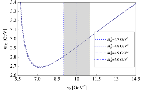
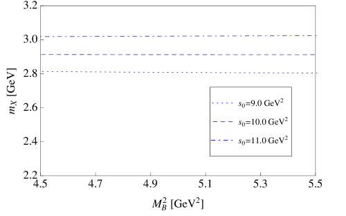
   Figure 1: Variation of the hadron mass $m_{X}$ with respect to $s_{0}$ and $M_{B}^{2}$ for $sq\bar{q}\bar{c}$ system with $J^{P}=0^{+}$ using the interpolating current $J_{2}(x)$.

   

   

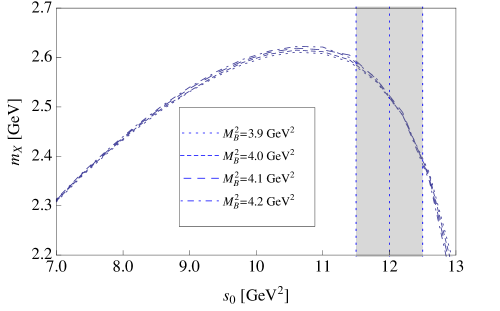
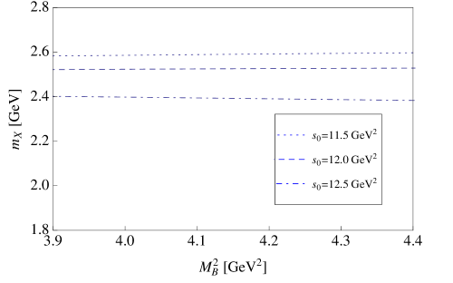
   Figure 2: Variation of the hadron mass $m_{X}$ with respect to $s_{0}$ and $M_{B}^{2}$ for $sq\bar{q}\bar{c}$ system with $J^{P}=0^{+}$ (S) using the interpolating current $J_{5\mu\nu}(x)$.

2. In this type we consider the traceless symmetric part of the interpolating current $J_{5\mu\nu}(x)$ in the scalar channel with $J^{P}=0^{+}$ (S). In the left panel of Fig . 2, we show the variation of the $m_{X}$ with respect to the continuum threshold $s_{0}$ in the Borel window $3.9\leq M_{B}^{2}\leq 4.2$ GeV². We find that the behaviour of these $s_{0}$-dependance curves is very different from those in type A as shown in Fig . 1. Instead of minimum points for type A, the $s_{0}$-dependance curves in type B have maximum points and then the extracted hadron mass decreases gradually with respect to $s_{0}$. However, we are still able to find the optimal values for the continuum threshold $11.5\leq s_{0}\leq 12.5$ GeV² to minimize the dependance of $m_{X}$ on the Borel mass $M_{B}^{2}$. In this working range, we plot the stable Borel curves in the right panel of Fig. 2 in the above Borel window, from which the extracted hadron mass decreases with respect to $s_{0}$. We finally obtain

   $$m_{X_{0^{+},\,S}^{cs}}=(2.52\pm 0.10\pm 0.11\pm 0.06\pm 0.05)\,\mbox{GeV}\,,$$ (18)

   in which the errors come from the uncertainties in the threshold values $s_{0}$, $M_{0}^{2}$, various QCD condensates and the charm quark mass, respectively.

3. In the third type we study the traceless antisymmetric part of the interpolating current $J_{5\mu\nu}(x)$ in the vector channel with $J^{P}=1^{-}$ (A). We first study the variation of the hadron mass with $s_{0}$ in its Borel window $2.6\leq M_{B}^{2}\leq 3.2$ GeV². As shown in the left panel of Fig. 3, the behaviour is totally different from those in types A and B. The extracted hadron mass $m_{X}$ increases monotonically with $s_{0}$ without any minimum or maximum point and the curves with different value of $M_{B}^{2}$ do not intersect anywhere. It seems that the mass sum rules are unstable in this situation. To explore the further behavior of $s_{0}$-dependance, we define the following hadron mass

   $$\overline{m}_{X}(s_{0})=\sum_{i=1}^{N}\frac{m_{X}(s_{0},M_{B,\ i}^{2})}{N}\,,$$ (19)

   in which the $M_{B,\ i}^{2}(i=1,2,\cdots,N)$ represent $N$ definite values for the Borel parameter $M_{B}^{2}$ in the Borel window $2.6\leq M_{B}^{2}\leq 3.2$ GeV². The $\overline{m}_{X}(s_{0})$ is defined as an averaged hadron mass for some definite value $M_{B}^{2}$. Using this average hadron mass, we can define the following quantity

   $$\chi^{2}(s_{0})=\sum_{i=1}^{N}\left[\frac{m_{X}(s_{0},M_{B,\ i}^{2})}{\overline{m}_{X}(s_{0})}-1\right]^{2}\,.$$ (20)

   According to the above definition, the optimal choice for the continuum threshold $s_{0}$ in the QCD sum rule analysis can be obtained by minimizing the quantity $\chi^{2}(s_{0})$, which is only the function of $s_{0}$. We show this relation in the right panel of Fig. 3, from which there is a minimum point around $s_{0}=13.5$ GeV². It is clearly that the $M_{B}^{2}$-dependance for the extracted hadron mass is the weakest at this point. We can thus determine the working range for the continuum threshold to be $12.0\leq s_{0}\leq 15.0$ GeV² in our analysis, as shown in the left panel of Fig. 3. In this area, we show $m_{X}$ as a function of the Borel parameter $M_{B}^{2}$ in Fig. 4 and predict the hadron mass at the central values $s_{0}=13.5$ GeV², $M_{B}^{2}=2.9$ GeV² to be

   $$m_{X_{1^{-},\,A}^{cs}}=(3.35\pm 0.14\pm 0.07\pm 0.04\pm 0.01)\,\mbox{GeV}\,,$$ (21)

   in which the errors come from the uncertainties in the threshold values $s_{0}$, $M_{0}^{2}$, various QCD condensates and the charm quark mass, respectively.

   

   

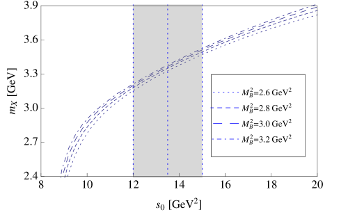
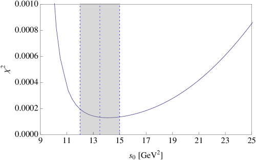
   Figure 3: Left panel: hadron mass $m_{X}$ as a function of $s_{0}$ for the $sq\bar{q}\bar{c}$ system using the traceless antisymmetric part of $J_{5\mu\nu}(x)$ with $J^{P}=1^{-}$(A). Right panel: the quantity $\chi^{2}$ as the function of the continuum threshold $s_{0}$.

   

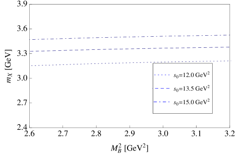
   Figure 4: Mass prediction for the $sq\bar{q}\bar{c}$ system with $J^{P}=1^{-}$(A).

$J^{PC}$	Currents	$s_{0}$(GeV2)	Borel window (GeV2)	$m_{X^{cs}}$(GeV)	Type
$0^{+}$	$J_{1}$	$7.5\pm 0.5$	$3.3-3.6$	$2.55\pm 0.10$	A
	$J_{2}$	$10.0\pm 0.5$	$4.7-5.0$	$2.91\pm 0.14$	A
	$J_{5\mu\nu}$(T)	$10.0\pm 0.5$	$2.2-3.1$	$2.88\pm 0.15$	A
	$J_{5\mu\nu}$(S)	$12.0\pm 0.5$	$3.9-4.2$	$2.53\pm 0.13$	B
$1^{+}$	$J_{3\mu}$	$7.5\pm 0.5$	$3.5-3.8$	$2.55\pm 0.12$	A
	$J_{4\mu}$	$9.5\pm 0.5$	$3.2-3.9$	$2.81\pm 0.13$	A
	$J_{5\mu\nu}$(A)	$9.5\pm 0.5$	$3.5-3.8$	$2.83\pm 0.13$	A
$2^{+}$	$J_{5\mu\nu}$(S)	$10.0\pm 0.5$	$3.4-4.0$	$2.91\pm 0.13$	A
$0^{-}$	$J_{3\mu}$	$7.5\pm 0.5$	$4.0-4.3$	$2.31\pm 0.09$	A
	$J_{4\mu}$	$12.0\pm 0.5$	$3.2-4.1$	$3.30\pm 0.16$	A
$1^{-}$	$J_{5\mu\nu}$(A)	$13.5\pm 1.0$	$2.6-3.4$	$3.35\pm 0.16$	C
	$J_{5\mu\nu}$(S)	$15.5\pm 1.0$	$3.2-3.9$	$3.55\pm 0.18$	C

Table 1: Mass spectrum for the charm-strange $sq\bar{q}\bar{c}$ tetraquark states.

For all interpolating currents in Eq. (1), we perform similar numerical analyses and collect the extracted hadron masses for the $sq\bar{q}\bar{c}$ tetraquark states in Table 1, together with the Borel windows and the working ranges for $s_{0}$. We show the three types introduced above in the last column. The error sources for the hadron masses include the uncertainties of the heavy quark masses, the QCD condensates, $M_{0}^{2}$, and the uncertainty of the continuum threshold $s_{0}$. As shown in Eqs. (17), (18) and (21), the uncertainty in $s_{0}$ is the dominant error source of the hadron mass while that of $M_{0}^{2}$ parameterizing the mixed condensate is also important. However, we list only the total errors in Table 1 with error analyses to summarize the results. In Table 1, we find that the extracted masses for the scalar $sq\bar{q}\bar{c}$ charmed tetraquarks with $J^{P}=0^{+}$ to be almost degenerate around $2.54$ GeV from the currents $J_{1}(x)$ and $J_{5\mu\nu}(x)$(S), while $2.90$ GeV from the currents $J_{2}(x)$ and $J_{5\mu\nu}(x)$(T). These values for the scalar charmed tetraquarks are higher than the mass of the charm-strange $D_{s0}^{\ast}(2317)$ meson. In addition, we obtain the hadron mass $m_{X_{cs}}=(2.55\pm 0.12)$ GeV for the axial-vector $sq\bar{q}\bar{c}$ tetraquark using the current $J_{3\mu}(x)$ with $J^{P}=1^{+}$. This result is not far from the mass of the narrow charm-strange $D_{s1}(2460)$ meson within the error.

Replacing the strange quark in $sq\bar{q}\bar{c}$ systems to be a down quark, we can study the non-strange charmed tetraquark systems $qq\bar{q}\bar{c}$ in similar way as the above analyses. The OPE series are a bit different by changing the condensates $\langle\bar{s}s\rangle$, $\langle\bar{s}Gs\rangle$ into $\langle\bar{q}q\rangle$, $\langle\bar{q}Gq\rangle$ respectively and neglecting the $m_{q}$ proportional terms in the chiral limit. The numerical results for these systems are then obtained and collected in Table 2. Similarly, we can easily study the strange and non-strange bottom tetraquark systems $sq\bar{q}\bar{b}$ and $qq\bar{q}\bar{b}$ in the heavy quark symmetry. After performing the QCD sum rule analyses, we collect the numerical results for the $sq\bar{q}\bar{b}$ and $qq\bar{q}\bar{b}$ systems in Tables 3 and 4, respectively. In Table 3, the masses for the bottom-strange $sq\bar{q}\bar{b}$ tetraquarks extracted from the interpolating currents $J_{1}(x)$ and $J_{3\mu}(x)$ were previously obtained in Ref. Chen et al. (2016b), which were used to explain the newly reported $X(5568)$ structure.

Except for the scalar and axial-vector states, we also investigate the other channels with $J^{P}=0^{-},1^{-},2^{+}$ and collect the results in Tables 1-4.

$J^{PC}$	Currents	$s_{0}$(GeV2)	Borel window (GeV2)	$m_{X^{cq}}$(GeV)	Type
$0^{+}$	$J_{1}$	$9.5\pm 0.5$	$3.1-4.0$	$2.82\pm 0.12$	A
	$J_{2}$	$10.0\pm 0.5$	$4.4-5.0$	$2.91\pm 0.13$	A
	$J_{5\mu\nu}$(T)	$10.5\pm 0.5$	$2.1-2.6$	$2.93\pm 0.13$	A
	$J_{5\mu\nu}$(S)	$8.5\pm 0.5$	$2.4-3.3$	$2.23\pm 0.12$	B
$1^{+}$	$J_{3\mu}$	$9.5\pm 0.5$	$3.3-3.9$	$2.83\pm 0.12$	A
	$J_{4\mu}$	$10.0\pm 0.5$	$3.0-4.2$	$2.88\pm 0.12$	A
	$J_{5\mu\nu}$(A)	$9.5\pm 0.5$	$3.3-3.9$	$2.82\pm 0.12$	A
$2^{+}$	$J_{5\mu\nu}$(S)	$10.0\pm 0.5$	$3.2-4.1$	$2.90\pm 0.15$	A
$0^{-}$	$J_{3\mu}$	$6.5\pm 0.5$	$4.1-4.4$	$2.21\pm 0.06$	A
	$J_{4\mu}$	$13.0\pm 0.5$	$3.4-4.0$	$3.29\pm 0.15$	C
$1^{-}$	$J_{5\mu\nu}$(A)	$13.5\pm 1.0$	$2.7-3.3$	$3.29\pm 0.16$	C
	$J_{5\mu\nu}$(S)	$15.5\pm 1.0$	$3.3-4.0$	$3.52\pm 0.17$	C

Table 2: Mass spectrum for the non-strange charmed $qq\bar{q}\bar{c}$ tetraquark states.

$J^{PC}$	Currents	$s_{0}$(GeV2)	Borel window (GeV2)	$m_{X^{bs}}$(GeV)	Type
$0^{+}$	$J_{1}$	$34.0\pm 2.0$	$6.0-6.3$	$5.59\pm 0.18$	A
	$J_{2}$	$37.0\pm 2.0$	$8.4-8.7$	$5.83\pm 0.21$	A
	$J_{5\mu\nu}$(T)	$41.0\pm 2.0$	$4.3-5.3$	$6.02\pm 0.21$	A
	$J_{5\mu\nu}$(S)	$61.0\pm 2.0$	$6.1-7.3$	$7.32\pm 0.21$	A
$1^{+}$	$J_{3\mu}$	$34.0\pm 2.0$	$6.3-6.6$	$5.59\pm 0.19$	A
	$J_{4\mu}$	$38.0\pm 2.0$	$6.0-7.3$	$5.86\pm 0.20$	A
	$J_{5\mu\nu}$(A)	$38.0\pm 2.0$	$6.3-7.4$	$5.88\pm 0.18$	A
$2^{+}$	$J_{5\mu\nu}$(S)	$40.0\pm 2.0$	$6.2-8.0$	$6.01\pm 0.22$	A
$0^{-}$	$J_{3\mu}$	$38.0\pm 2.0$	$6.6-6.9$	$5.62\pm 0.24$	A
	$J_{4\mu}$	$43.0\pm 2.0$	$5.5-6.7$	$6.32\pm 0.18$	A
$1^{-}$	$J_{5\mu\nu}$(A)	$43.0\pm 2.0$	$4.4-5.0$	$6.19\pm 0.25$	C
	$J_{5\mu\nu}$(S)	$44.0\pm 2.0$	$4.8-5.5$	$6.22\pm 0.27$	C

Table 3: Mass spectrum for the bottom-strange $sq\bar{q}\bar{b}$ tetraquark states.

$J^{PC}$	Currents	$s_{0}$(GeV2)	Borel window (GeV2)	$m_{X^{bq}}$(GeV)	Type
$0^{+}$	$J_{1}$	$38.0\pm 2.0$	$5.8-7.4$	$5.86\pm 0.20$	A
	$J_{2}$	$37.0\pm 2.0$	$8.0-8.3$	$5.83\pm 0.20$	A
	$J_{5\mu\nu}$(T)	$41.0\pm 2.0$	$4.3-5.3$	$6.02\pm 0.21$	A
	$J_{5\mu\nu}$(S)	$52.0\pm 2.0$	$5.1-5.6$	$6.74\pm 0.24$	C
$1^{+}$	$J_{3\mu}$	$38.0\pm 2.0$	$6.1-7.4$	$5.87\pm 0.21$	A
	$J_{4\mu}$	$40.0\pm 2.0$	$5.8-6.7$	$5.98\pm 0.21$	A
	$J_{5\mu\nu}$(A)	$38.0\pm 2.0$	$6.1-7.4$	$5.86\pm 0.21$	A
$2^{+}$	$J_{5\mu\nu}$(S)	$40.0\pm 2.0$	$6.0-6.7$	$5.99\pm 0.21$	A
$0^{-}$	$J_{3\mu}$	$37.0\pm 2.0$	$6.8-7.1$	$5.51\pm 0.25$	A
	$J_{4\mu}$	$44.0\pm 2.0$	$5.6-6.0$	$6.23\pm 0.24$	C
$1^{-}$	$J_{5\mu\nu}$(A)	$40.0\pm 2.0$	$4.1-4.7$	$5.88\pm 0.27$	C
	$J_{5\mu\nu}$(S)	$41.0\pm 2.0$	$4.5-5.0$	$5.94\pm 0.27$	C

Table 4: Mass spectrum for the non-strange bottom $qq\bar{q}\bar{b}$ tetraquark states.

IV Decay properties of the open-flavor charmed/bottom tetraquarks

Using the mass spectra obtained above, we can study the possible decay patterns of the $sq\bar{q}\bar{c}$, $qq\bar{q}\bar{c}$, $sq\bar{q}\bar{b}$, $qq\bar{q}\bar{b}$ tetraquark states in various channels. These open-flavor charmed/bottom tetraquarks will decay easily through the fall-apart mechanism so long as the kinematics allows. We study both the S-wave and P-wave two-body hadronic decays by considering the conservation of the angular momentum, parity and isospin in Tables 5 and 6.

In Table 5, we list the possible S-wave two-body hadronic decay modes for the $sq\bar{q}\bar{c}$, $qq\bar{q}\bar{c}$, $sq\bar{q}\bar{b}$, $qq\bar{q}\bar{b}$ tetraquark states with various quantum numbers. We consider isospin-0/1 for $sq\bar{q}\bar{c}$, $sq\bar{q}\bar{b}$ states and isospin-$\frac{1}{2}$/$\frac{3}{2}$ for $qq\bar{q}\bar{c}$, $qq\bar{q}\bar{b}$ states, respectively. In the chiral limit, these tetraquarks in the same isospin multiplet are predicted to be degenerate since we do not differentiate between the up and down quarks. For the charmed/bottom-strange $sq\bar{q}\bar{c}$ and $sq\bar{q}\bar{b}$ states, their decay patterns are very different for the isospin-scalar and isospin-vector channels except some one $D/B$ meson plus one $K$ meson decay modes. Such decays are allowed by the isospin symmetry for both channels. However, the situation is different for the non-strange $qq\bar{q}\bar{c}$ and $qq\bar{q}\bar{b}$ tetraquarks. In Table 5, one notes that all possible decay modes for the isospin-$\frac{3}{2}$ states are allowed for the corresponding isospin-$\frac{1}{2}$ ones.

As shown in Table 5, there is no allowed S-wave decay modes for the tensor $sq\bar{q}\bar{b}$ states. This is because the predicted hadron mass for these tetraquarks in Table 3 is lower than any possible S-wave two-body hadronic decay threshold. There also exist some other tetraquark states below the S-wave decay thresholds, which are denoted by “$-$” in Table 5. However, it is shown that the P-wave decays are allowed for these states, as shown in Table 6. This means that the P-wave decay modes are dominant for these tetraquark states and thus they are much narrower than other states. These tetraquark states will be prime candidates for observation.

$I(J^{P})$	$sq\bar{q}\bar{b}$	$sq\bar{q}\bar{c}$	$I(J^{P})$	$qq\bar{q}\bar{b}$	$qq\bar{q}\bar{c}$
$0(0^{+})$	$B_{s}^{0}\eta/\eta^{\prime}$, $B_{s}^{\ast}\omega/\phi$, $B^{\ast}K^{\ast}(892)$,	$D_{s}\eta/\eta^{\prime}$,	$\frac{1}{2}(0^{+})$	$B\eta/\eta^{\prime}$, $B^{\ast}\omega/\phi$,	$D\pi/\eta/\eta^{\prime}$,
	$B_{s1}(5830)^{0}h_{1}(1170)/f_{1}(1285)$,	$D_{s}^{\ast}\omega$,		$B\pi$, $B^{\ast}\rho$	$D^{\ast}\omega/\rho$
	$B_{1}(5721)^{0}K_{1}(1270)$, $BK$	$DK$
$1(0^{+})$	$B_{s}^{0}\pi$, $BK$, $B_{s}^{\ast}\rho$, $B^{\ast}K^{\ast}(892)$,	$D_{s}\pi$,	$\frac{3}{2}(0^{+})$	$B\pi$, $B^{\ast}\rho$	$D\pi$,
	$B_{s1}(5830)^{0}b_{1}(1235)/a_{1}(1260)$,	$D_{s}^{\ast}\rho$,			$D^{\ast}\rho$
	$B_{1}(5721)^{0}K_{1}(1270)$	$DK$
$0(1^{+})$	$-$	$-$	$\frac{1}{2}(1^{+})$	$B^{\ast}\pi$, $B\omega$	$D^{\ast}\pi$, $D\omega/\rho$
$1(1^{+})$	$B_{s}^{\ast}\pi$	$D_{s}^{\ast}\pi$	$\frac{3}{2}(1^{+})$	$B^{\ast}\pi$, $B\rho$	$D^{\ast}\pi$, $D\rho$
$0(2^{+})$	$-$	$D_{s}^{\ast}\omega$	$\frac{1}{2}(2^{+})$	$-$	$D^{\ast}(2007)^{0}\omega/\rho$
$1(2^{+})$	$-$	$D_{s}^{\ast}\rho$	$\frac{3}{2}(2^{+})$	$-$	$D^{\ast}(2007)^{0}\rho$
$0(0^{-})$	$B_{s}^{0}\sigma$	$D_{s}\sigma/f_{0}(980)$	$\frac{1}{2}(0^{-})$	$B\sigma$	$D\sigma/a_{0}/f_{0}$, $D_{0}^{\ast}(2400)\pi$
$1(0^{-})$	$-$	$D_{s}a_{0}(980)$, $D_{s0}^{\ast}(2317)\pi$	$\frac{3}{2}(0^{-})$	$-$	$Da_{0}(980)$, $D_{0}^{\ast}(2400)\pi$
$0(1^{-})$	$-$	$D_{s}h_{1}(1170)/f_{1}(1285)$,	$\frac{1}{2}(1^{-})$	$B_{1}(5721)^{0}\pi$	$Dh_{1}/f_{1}/a_{1}/b_{1}$, $D_{0}^{\ast}\omega/\rho$,
		$D_{s}^{\ast}\sigma/f_{0}(980)$, $D_{s0}^{\ast}(2317)\omega$,			$D^{\ast}\sigma/f_{0}/a_{0}$, $D^{\ast}h_{1}/b_{1}$,
		$D_{s1}(2536)\omega$, $D_{s}^{\ast}h_{1}(1170)$			$D_{1}(2420)^{0}\omega/\rho/\pi$
$1(1^{-})$	$B_{s1}(5830)^{0}\pi$	$D_{s}b_{1}(1235)/a_{1}(1260)$,	$\frac{3}{2}(1^{-})$	$B_{1}(5721)^{0}\pi$	$D^{\ast}a_{0}$, $Da_{1}/b_{1}$, $D_{0}^{\ast}\rho$,
		$D_{s1}(2460)\pi$, $D_{s0}^{\ast}(2317)\rho$,			$D_{0}^{\ast}(2400)\pi/\rho$,
		$D_{s}^{\ast}a_{0}(980)$, $D_{s1}(2536)\rho$			$D^{\ast}(2007)^{0}b_{1}$

Table 5: Possible S-wave decay modes for the open-flavor charmed/bottom tetraquark states where ‘$-$’ denotes that the predicted tetraquark masses are below all allowed S-wave two-body hadronic decay thresholds.

$I(J^{P})$	$sq\bar{q}\bar{b}$	$sq\bar{q}\bar{c}$	$I(J^{P})$	$qq\bar{q}\bar{b}$	$qq\bar{q}\bar{c}$
$0(0^{+})$	$B_{s}^{0}h_{1}/f_{1}$, $B_{s}^{\ast}\sigma/f_{0}$, $BK_{1}(1270)$,	$D_{s}^{\ast}\sigma$	$\frac{1}{2}(0^{+})$	$Bh_{1}/f_{1}/b_{1}/a_{1}$,	$D_{1}(2420)\pi$, $D^{\ast}\sigma$,
	$B_{s1}(5830)^{0}\omega/\phi$, $B_{s}^{\ast}h_{1}/f_{1}$,			$B^{\ast}\sigma/f_{0}/h_{1}/b_{1}/a_{1}$,
	$B_{1}(5721)^{0}K^{\ast}(892)$, $B^{\ast}K_{1}/K_{0}^{\ast}$			$B_{1}(5721)^{0}\pi/\rho/\omega/\phi$
$1(0^{+})$	$B_{s1}(5830)^{0}\pi/\rho$, $B_{s}^{\ast}a_{0}$, $BK_{1}$,	$D_{s1}(2460)\pi$	$\frac{3}{2}(0^{+})$	$Bb_{1}/a_{1}$,	$D_{1}(2420)\pi$,
	$B_{s}^{0}b_{1}/a_{1}$, $B_{s}^{\ast}a_{0}/b_{1}/a_{1}$,			$B^{\ast}a_{0}/b_{1}/a_{1}$,
	$B_{1}(5721)^{0}K^{\ast}(892)$, $B^{\ast}K_{1}/K_{0}^{\ast}$			$B_{1}(5721)^{0}\pi/\rho$
$0(1^{+})$	$B_{s}^{0}/B_{s}^{\ast}\sigma$	$D_{s}/D_{s}^{\ast}\sigma$	$\frac{1}{2}(1^{+})$	$B/B^{\ast}\sigma$, $B_{1}(5721)^{0}\pi$	$D_{1}(2420)\pi$, $D/D^{\ast}\sigma$
$1(1^{+})$	$B_{s1}(5830)^{0}\pi$	$D_{s1}(2460)\pi$	$\frac{3}{2}(1^{+})$	$B_{1}(5721)^{0}\pi$	$D_{1}(2420)\pi$
$0(2^{+})$	$B_{s}^{\ast}\sigma$	$D_{s}^{\ast}\sigma$	$\frac{1}{2}(2^{+})$	$B^{\ast}\sigma$, $B_{1}(5721)^{0}\pi$	$D_{1}(2420)\pi$, $D^{\ast}\sigma$
$1(2^{+})$	$B_{s1}(5830)^{0}\pi$	$D_{s1}(2460)\pi$	$\frac{3}{2}(2^{+})$	$B_{1}(5721)^{0}\pi$	$D_{1}(2420)\pi$
$0(0^{-})$	$B_{s}^{0}\omega$, $B_{s}^{\ast}\eta/\eta^{\prime}/\omega$,	$D_{s}\omega$, $D_{s}^{\ast}\eta/\eta^{\prime}\omega$, $D_{s1}\sigma$,	$\frac{1}{2}(0^{-})$	$B^{\ast}\pi/\eta/\eta^{\prime}$,	$D\rho/\omega/\phi$, $D^{\ast}\pi/\eta/\eta^{\prime}$,
	$B^{\ast}K$, $B/B^{\ast}K^{\ast}$	$D^{\ast}K$, $D/D^{\ast}K^{\ast}$		$B\rho/\omega$, $B^{\ast}\rho/\omega$	$D^{\ast}\rho/\omega/\phi$, $D_{1}(2420)\sigma$
$1(0^{-})$	$B_{s}^{0}\rho$, $B_{s}^{\ast}\pi/\rho$, $B^{\ast}K$, $B/B^{\ast}K^{\ast}$	$D_{s}\rho$, $D_{s}^{\ast}\pi/\rho$, $D^{\ast}K$, $D/D^{\ast}K^{\ast}$	$\frac{3}{2}(0^{-})$	$B^{\ast}\pi/\rho,B\rho$	$D/D^{\ast}\rho$, $D^{\ast}\pi$
$0(1^{-})$	$B_{s}^{0}\omega,BK$,	$D_{s}\eta/\eta^{\prime}/\omega$, $D_{s}^{\ast}\omega/\eta/\eta^{\prime}$, $D_{s1}\sigma$,	$\frac{1}{2}(1^{-})$	$B/B^{\ast}\pi$	$D\pi/\eta/\eta^{\prime}/\rho/\omega/\phi$,
		$D/D^{\ast}K$, $D/D^{\ast}K^{\ast}$			$D^{\ast}\pi/\eta/\eta^{\prime}/\rho/\omega/\phi$
$1(1^{-})$	$B_{s}^{\ast}\pi$, $B_{s}^{0}\rho/\pi,BK$	$D_{s}\pi/\rho$, $D_{s}^{\ast}\pi/\rho$,	$\frac{3}{2}(1^{-})$	$B/B^{\ast}\pi$	$D\pi/\rho$, $D^{\ast}\pi/\rho$
		$D/D^{\ast}K$, $D/D^{\ast}K^{\ast}$

Table 6: Possible P-wave decay modes for the open-flavor charmed/bottom tetraquark states.

V Conclusions and discussion

In this paper, we have studied the open-flavor charmed/bottom $sq\bar{q}\bar{c}$, $qq\bar{q}\bar{c}$, $sq\bar{q}\bar{b}$, $qq\bar{q}\bar{b}$ tetraquark states with the spin-parity quantum numbers $J^{P}=0^{+},1^{+},2^{+}$ and $0^{-},1^{-}$. In the diquark configurations, we use only the color-antisymmetric scalar and axial-vector diquarks to compose the color-antisymmetric $[\mathbf{\bar{3}_{c}}]_{diquark}\otimes[\mathbf{3_{c}}]_{antidiquark}$ tetraquark interpolating currents. Finally, we obtain five tetraquark currents in Eq. (1) with various spin-parity quantum numbers.

After performing the numerical analyses, we obtained the hadron masses for the open-flavor charmed/bottom $sq\bar{q}\bar{c}$, $qq\bar{q}\bar{c}$, $sq\bar{q}\bar{b}$, $qq\bar{q}\bar{b}$ tetraquark states. For the charm-strange $sq\bar{q}\bar{c}$ systems, we extract the hadron mass $m_{X_{cs}}=(2.55\pm 0.12)$ GeV using the interpolating current $J_{3\mu}(x)$ with $J^{P}=1^{+}$, which is not far from the mass of the $D_{s1}(2460)$ meson within the error. In the scalar channel, however, the results for the $sq\bar{q}\bar{c}$ systems disfavor the tetraquark explanation of the charm-strange $D_{s0}^{\ast}(2317)$ meson.

Our results indicate that many other charmed/bottom tetraquarks may exist, and we have evaluated their masses. The tetraquarks $[su][\bar{d}\bar{c}]$, $\frac{[su][\bar{u}\bar{c}]+[sd][\bar{d}\bar{c}]}{\sqrt{2}}$, and $[sd][\bar{u}\bar{c}]$ can form an iso-triplet. Since we do not differentiate the up and down quarks in the OPE series, these tetraquark states in the same isospin multiplet have the same extracted hadron masses in our analyses. In other words, the mass spectra in Tables 1–4 contain all open-flavor charmed/bottom tetraquarks. Among these states, the exotic doubly-charged tetraquarks, such as $[sd][\bar{u}\bar{c}]\to D_{s}^{(\ast)-}\pi^{-}$, is especially interesting, and have not been observed so far. Our results for their mass spectra can be useful for their searches in future experiments at facilities such as BESIII, BelleII, PANDA, LHCb, CMS, etc.

Appendix A Spectral densities

In this appendix, we collect the spectral densities for all interpolating currents defined in Eq. (1). To calculate these spectral densities, we use the momentum space propagators for the heavy quarks (bottom and charm) and strange quark while coordinate space propagators for the light quarks

$$\begin{split}iS_{Q}^{ab}&=\frac{i\delta^{ab}}{\hat{p}-m_{Q}}+\frac{i}{4}g_{s}\frac{\lambda^{n}_{ab}}{2}G^{n}_{\mu\nu}\frac{\sigma^{\mu\nu}(\hat{p}+m_{Q})+(\hat{p}+m_{Q})\sigma^{\mu\nu}}{(p^{2}-m_{Q}^{2})^{2}}+\frac{i\delta^{ab}}{12}\langle g^{2}_{s}GG\rangle m_{Q}\frac{p^{2}+m_{Q}\hat{p}}{(p^{2}-m_{Q}^{2})^{4}}\,,\\ iS_{q}^{ab}&=\frac{i\delta^{ab}}{2\pi^{2}x^{4}}\hat{x}+\frac{i}{32\pi^{2}}\frac{\lambda^{n}_{ab}}{2}g_{s}G^{n}_{\mu\nu}\frac{1}{x^{2}}(\sigma^{\mu\nu}\hat{x}+\hat{x}\sigma^{\mu\nu})-\frac{\delta^{ab}}{12}\langle\bar{q}q\rangle+\frac{\delta^{ab}x^{2}}{192}\langle g_{s}\bar{q}\sigma\cdot Gq\rangle-\frac{m_{q}\delta^{ab}}{4\pi^{2}x^{2}}+\frac{i\delta^{ab}m_{q}\langle\bar{q}q\rangle}{48}\hat{x}\,,\end{split}$$ (22)

where $\hat{x}=\gamma_{\mu}x^{\mu}$, $\hat{p}=\gamma_{\mu}p^{\mu}$. The nonperturbative terms correlated to $\langle\bar{s}s\rangle$ and $\langle\bar{s}g_{s}\sigma\cdot Gs\rangle$ are also calculated by considering the various strange quark condensates. We will use the projectors defined in Eq. (6) to pick out the different invariant functions and also the spectral densities for the vector and tensor currents. Up to dimension eight, the spectral density can be written as

$$\rho(s)=\rho^{pert}(s)+\rho^{\langle\bar{q}q\rangle}(s)+\rho^{\langle GG\rangle}(s)+\rho^{\langle\bar{q}Gq\rangle}(s)+\rho^{\langle\bar{q}q\rangle^{2}}(s)+\rho^{\langle\bar{q}q\rangle\langle\bar{q}Gq\rangle}\,.$$ (23)

• For the current $J_{1}(x)$ with $J^{P}=0^{+}$

  $$\rho^{pert}_{1}(s) =\frac{1}{512\pi^{6}}\int^{\alpha_{max}}_{\alpha_{min}}d\alpha\int^{\beta_{max}}_{\beta_{min}}d\beta\frac{(1-\alpha-\beta)^{2}(\alpha m_{s}^{2}+\beta m_{Q}^{2}-\alpha\beta s)^{3}(\alpha m_{s}^{2}+\beta m_{Q}^{2}-3\alpha\beta s)}{\alpha^{3}\beta^{3}}\,,$$

  $$\rho^{\langle\bar{q}q\rangle}_{1}(s) =-\frac{\langle\bar{q}q\rangle}{16\pi^{4}}\int^{\alpha_{max}}_{\alpha_{min}}d\alpha\int^{\beta_{max}}_{\beta_{min}}d\beta\left(\frac{m_{Q}}{\alpha}+\frac{m_{s}}{\beta}\right)\frac{(1-\alpha-\beta)(\alpha m_{s}^{2}+\beta m_{Q}^{2}-\alpha\beta s)(\alpha m_{s}^{2}+\beta m_{Q}^{2}-2\alpha\beta s)}{\alpha\beta}\,,$$

  $$\rho^{\langle\bar{s}s\rangle}_{1}(s) =\frac{m_{s}\langle\bar{s}s\rangle(s-m_{Q}^{2})(s^{2}-5m_{Q}^{2}s-2m_{Q}^{4})}{384\pi^{4}s}-\frac{m_{Q}^{4}m_{s}\langle\bar{s}s\rangle\log[m_{Q}^{2}/s]}{64\pi^{4}}\,,$$

  $$\rho^{\langle GG\rangle}_{1}(s) =\frac{\langle g_{s}^{2}GG\rangle}{1024\pi^{6}}\int^{\alpha_{max}}_{\alpha_{min}}d\alpha\int^{\beta_{max}}_{\beta_{min}}d\beta\Bigg{[}\left(\frac{m_{Q}^{2}}{\alpha^{3}}+\frac{m_{s}^{2}}{\beta^{3}}\right)\frac{(1-\alpha-\beta)^{2}(2\alpha m_{s}^{2}+2\beta m_{Q}^{2}-3\alpha\beta s)}{3}$$

  $$+\left(\frac{1}{\alpha}+\frac{1}{\beta}\right)\frac{(1-\alpha-\beta)(\alpha m_{s}^{2}+\beta m_{Q}^{2}-\alpha\beta s)(\alpha m_{s}^{2}+\beta m_{Q}^{2}-2\alpha\beta s)}{\alpha\beta}\Bigg{]}\,,$$

  $$\rho^{\langle\bar{q}Gq\rangle}_{1}(s) =\frac{\langle\bar{q}g_{s}\sigma\cdot Gq\rangle}{64\pi^{4}}\int^{\alpha_{max}}_{\alpha_{min}}d\alpha\int^{\beta_{max}}_{\beta_{min}}d\beta\Bigg{[}\left(\frac{m_{Q}}{\alpha}+\frac{m_{s}}{\beta}\right)$$ (24)

  $$-\left(\frac{m_{Q}}{\alpha^{2}}+\frac{m_{s}}{\beta^{2}}\right)(1-\alpha-\beta)\Bigg{]}(2\alpha m_{s}^{2}+2\beta m_{Q}^{2}-3\alpha\beta s)\,,$$

  $$\rho^{\langle\bar{q}q\rangle^{2}}_{1}(s) =\frac{m_{Q}m_{s}\langle\bar{q}q\rangle^{2}}{12\pi^{2}}\sqrt{\left(1-\frac{m_{Q}^{2}-m_{s}^{2}}{s}\right)^{2}-\frac{4m_{s}^{2}}{s}}+\frac{\langle\bar{q}q\rangle\langle\bar{s}s\rangle(s-m_{Q}^{2})(s-m_{Q}m_{s}-m_{Q}^{2})}{24\pi^{2}s}\,,$$

  $$\rho^{\langle\bar{q}q\rangle\langle\bar{q}Gq\rangle}_{1}(s) =\frac{\langle\bar{s}s\rangle\langle\bar{q}g_{s}\sigma\cdot Gq\rangle+\langle\bar{q}q\rangle\langle\bar{s}g_{s}\sigma\cdot Gs\rangle}{48\pi^{2}}$$

  $$+\frac{m_{Q}m_{s}\langle\bar{q}q\rangle\langle\bar{q}g_{s}\sigma\cdot Gq\rangle}{48\pi^{2}}\int_{0}^{1}d\alpha\Bigg{[}\frac{2m_{s}^{2}}{\alpha^{2}}\delta^{\prime}\left(s-\tilde{m}^{2}_{Q}\right)-\frac{1}{\alpha(1-\alpha)}\delta\left(s-\tilde{m}^{2}_{Q}\right)\Bigg{]}\,.$$

  in which

  $$\alpha_{max} =\frac{1}{2}\left[1+\frac{m_{Q}^{2}-m_{s}^{2}}{s}+\sqrt{\left(1+\frac{m_{Q}^{2}-m_{s}^{2}}{s}\right)^{2}-\frac{4m_{Q}^{2}}{s}}\right]\,,$$

  $$\alpha_{min} =\frac{1}{2}\left[1+\frac{m_{Q}^{2}-m_{s}^{2}}{s}-\sqrt{\left(1+\frac{m_{Q}^{2}-m_{s}^{2}}{s}\right)^{2}-\frac{4m_{Q}^{2}}{s}}\right]\,,$$

  $$\beta_{max} =\frac{m_{s}^{2}\alpha}{s\alpha-m_{Q}^{2}}\,,$$ (25)

  $$\beta_{min} =1-\alpha\,,$$

  $$\tilde{m}^{2}_{Q} =\frac{m_{Q}^{2}\alpha+m_{s}^{2}(1-\alpha)}{\alpha(1-\alpha)}\,.$$

• For the current $J_{2}(x)$ with $J^{P}=0^{+}$

  $$\rho^{pert}_{2}(s) =4\rho^{pert}_{1}(s),\,\rho^{\langle\bar{q}q\rangle}_{2}(s)=8\rho^{\langle\bar{q}q\rangle}_{1}(s),\,\rho^{\langle\bar{s}s\rangle}_{2}(s)=4\rho^{\langle\bar{s}s\rangle}_{1}(s)\,,$$

  $$\rho^{\langle GG\rangle}_{2}(s) =\frac{\langle g_{s}^{2}GG\rangle}{256\pi^{6}}\int^{\alpha_{max}}_{\alpha_{min}}d\alpha\int^{\beta_{max}}_{\beta_{min}}d\beta\Bigg{[}\left(\frac{m_{Q}^{2}}{\alpha^{3}}+\frac{m_{s}^{2}}{\beta^{3}}\right)\frac{(1-\alpha-\beta)^{2}(2\alpha m_{s}^{2}+2\beta m_{Q}^{2}-3\alpha\beta s)}{3}$$

  $$-\left(\frac{1}{\alpha}+\frac{1}{\beta}\right)\frac{(1-\alpha-\beta)(\alpha m_{s}^{2}+\beta m_{Q}^{2}-\alpha\beta s)(\alpha m_{s}^{2}+\beta m_{Q}^{2}-2\alpha\beta s)}{\alpha\beta}\Bigg{]}\,,$$

  $$\rho^{\langle\bar{q}Gq\rangle}_{2}(s) =\frac{\langle\bar{q}g_{s}\sigma\cdot Gq\rangle}{8\pi^{4}}\int^{\alpha_{max}}_{\alpha_{min}}d\alpha\int^{\beta_{max}}_{\beta_{min}}d\beta\left(\frac{m_{Q}}{\alpha}+\frac{m_{s}}{\beta}\right)(2\alpha m_{s}^{2}+2\beta m_{Q}^{2}-3\alpha\beta s)\,,$$ (26)

  $$\rho^{\langle\bar{q}q\rangle^{2}}_{2}(s) =\frac{4m_{Q}m_{s}\langle\bar{q}q\rangle^{2}}{3\pi^{2}}\sqrt{\left(1-\frac{m_{Q}^{2}-m_{s}^{2}}{s}\right)^{2}-\frac{4m_{s}^{2}}{s}}+\frac{\langle\bar{q}q\rangle\langle\bar{s}s\rangle(s-m_{Q}^{2})(s-m_{Q}m_{s}-m_{Q}^{2})}{3\pi^{2}s}\,,$$

  $$\rho^{\langle\bar{q}q\rangle\langle\bar{q}Gq\rangle}_{2}(s) =\frac{\langle\bar{s}s\rangle\langle\bar{q}g_{s}\sigma\cdot Gq\rangle+\langle\bar{q}q\rangle\langle\bar{s}g_{s}\sigma\cdot Gs\rangle}{6\pi^{2}}+\frac{2m_{Q}m_{s}^{3}\langle\bar{q}q\rangle\langle\bar{q}g_{s}\sigma\cdot Gq\rangle}{3\pi^{2}}\int_{0}^{1}d\alpha\frac{1}{\alpha^{2}}\delta^{\prime}\left(s-\tilde{m}^{2}_{Q}\right)\,.$$

• For the trace of current $J_{5\mu\nu}(x)$ with $J^{P}=0^{+}$(T)

  $$\rho^{pert}_{3}(s) =\frac{1}{4}\rho^{pert}_{1}(s),\,\rho^{\langle\bar{q}q\rangle}_{3}(s)=\frac{1}{8}\rho^{\langle\bar{q}q\rangle}_{1}(s),\,\rho^{\langle\bar{s}s\rangle}_{3}(s)=\frac{1}{4}\rho^{\langle\bar{s}s\rangle}_{1}(s)\,,$$

  $$\rho^{\langle GG\rangle}_{3}(s) =\frac{\langle g_{s}^{2}GG\rangle}{4096\pi^{6}}\int^{\alpha_{max}}_{\alpha_{min}}d\alpha\int^{\beta_{max}}_{\beta_{min}}d\beta\Bigg{[}\frac{(1-\beta)(\alpha m_{s}^{2}+\beta m_{Q}^{2}-\alpha\beta s)(\alpha m_{s}^{2}+\beta m_{Q}^{2}-2\alpha\beta s)}{4\alpha^{2}\beta}$$

  $$+\frac{m_{Q}^{2}(1-\alpha-\beta)^{2}(2\alpha m_{s}^{2}+2\beta m_{Q}^{2}-3\alpha\beta s)}{3\alpha^{3}}\Bigg{]}\,,$$

  $$\rho^{\langle\bar{q}Gq\rangle}_{3}(s) =\frac{\langle\bar{q}g_{s}\sigma\cdot Gq\rangle}{2048\pi^{4}}\int^{\alpha_{max}}_{\alpha_{min}}d\alpha\int^{\beta_{max}}_{\beta_{min}}d\beta(2\alpha m_{s}^{2}+2\beta m_{Q}^{2}-3\alpha\beta s)$$ (27)

  $$\Bigg{[}3\left(\frac{m_{Q}}{\alpha}+\frac{m_{s}}{\beta}\right)+\frac{(m_{Q}-m_{s})(1-\alpha-\beta)}{\alpha\beta}\Bigg{]}\,,$$

  $$\rho^{\langle\bar{q}q\rangle^{2}}_{3}(s) =\frac{m_{Q}m_{s}\langle\bar{q}q\rangle^{2}}{48\pi^{2}}\sqrt{\left(1-\frac{m_{Q}^{2}-m_{s}^{2}}{s}\right)^{2}-\frac{4m_{s}^{2}}{s}}+\frac{\langle\bar{q}q\rangle\langle\bar{s}s\rangle(s-m_{Q}^{2})(s-m_{Q}m_{s}-m_{Q}^{2})}{192\pi^{2}s}\,,$$

  $$\rho^{\langle\bar{q}q\rangle\langle\bar{q}Gq\rangle}_{3}(s) =\frac{\langle\bar{s}s\rangle\langle\bar{q}g_{s}\sigma\cdot Gq\rangle}{384\pi^{2}}+\frac{\langle\bar{q}q\rangle\langle\bar{s}g_{s}\sigma\cdot Gs\rangle}{768\pi^{2}}+\frac{m_{Q}^{2}\langle\bar{q}q\rangle\langle\bar{s}g_{s}\sigma\cdot Gs\rangle}{1536\pi^{2}s}$$

  $$+\frac{m_{Q}m_{s}\langle\bar{q}q\rangle\langle\bar{q}g_{s}\sigma\cdot Gq\rangle}{768\pi^{2}}\int_{0}^{1}d\alpha\Bigg{[}\frac{8m_{s}^{2}}{\alpha^{2}}\delta^{\prime}\left(s-\tilde{m}^{2}_{Q}\right)-\frac{1}{\alpha(1-\alpha)}\delta\left(s-\tilde{m}^{2}_{Q}\right)\Bigg{]}\,.$$

• For the traceless symmetric part of the current $J_{5\mu\nu}(x)$ with $J^{P}=0^{+}$(S)

  $$\rho^{pert}_{4}(s) =\frac{1}{128\pi^{6}}\int^{\alpha_{max}}_{\alpha_{min}}d\alpha\int^{\beta_{max}}_{\beta_{min}}d\beta(1-\alpha-\beta)^{2}(\alpha m_{s}^{2}+\beta m_{Q}^{2}-\alpha\beta s)^{2}\Bigg{[}\frac{(1-\alpha-\beta)(\alpha m_{s}^{2}+\beta m_{Q}^{2}-5\alpha\beta s)^{2}}{8\alpha^{3}\beta^{3}}$$

  $$-\frac{(1-\alpha-\beta)(\alpha m_{s}^{2}+\beta m_{Q}^{2}-\alpha\beta s)^{2}s}{\alpha^{2}\beta^{2}}-\frac{(\alpha m_{s}^{2}+\beta m_{Q}^{2}-\alpha\beta s)(\alpha m_{s}^{2}+\beta m_{Q}^{2}-27\alpha\beta s)}{16\alpha^{3}\beta^{3}}\Bigg{]}\,,$$

  $$\rho^{\langle\bar{q}q\rangle}_{4}(s) =-\frac{3\langle\bar{q}q\rangle}{128\pi^{4}}\int^{\alpha_{max}}_{\alpha_{min}}d\alpha\int^{\beta_{max}}_{\beta_{min}}d\beta\left(\frac{m_{Q}}{\alpha}+\frac{m_{s}}{\beta}\right)\frac{(1-\alpha-\beta)(\alpha m_{s}^{2}+\beta m_{Q}^{2}-\alpha\beta s)(\alpha m_{s}^{2}+\beta m_{Q}^{2})}{\alpha\beta}\,,$$

  $$\rho^{\langle\bar{s}s\rangle}_{4}(s) =\frac{m_{s}\langle\bar{s}s\rangle(s-m_{Q}^{2})(9s^{4}-45m_{Q}^{2}s^{3}-29m_{Q}^{4}s^{2}+7m_{Q}^{6}s-2m_{Q}^{8})}{1536\pi^{4}s^{3}}-\frac{5m_{Q}^{4}m_{s}\langle\bar{s}s\rangle\log[m_{Q}^{2}/s]}{128\pi^{4}}\,,$$

  $$\rho^{\langle GG\rangle}_{4}(s) =\frac{\langle g_{s}^{2}GG\rangle}{1024\pi^{6}}\int^{\alpha_{max}}_{\alpha_{min}}d\alpha\int^{\beta_{max}}_{\beta_{min}}d\beta\Bigg{\{}-\frac{(1-\alpha-\beta)(\alpha m_{s}^{2}+\beta m_{Q}^{2}-\alpha\beta s)(17\alpha m_{s}^{2}+17\beta m_{Q}^{2}-46\alpha\beta s)}{48\alpha^{2}\beta}$$

  $$+\frac{m_{Q}^{2}(1-\alpha-\beta)^{2}(2\alpha m_{s}^{2}+2\beta m_{Q}^{2}-3\alpha\beta s)}{4\alpha^{3}}-\frac{m_{Q}^{2}(1-\alpha-\beta)^{3}(\alpha m_{s}^{2}+\beta m_{Q}^{2}-3\alpha\beta s)}{3\alpha^{3}}$$

  $$+\frac{(1-\alpha-\beta)^{2}\left[9(\alpha m_{s}^{2}+\beta m_{Q}^{2}-\alpha\beta s)^{2}-78\alpha\beta s(\alpha m_{s}^{2}+\beta m_{Q}^{2}-\alpha\beta s)+28\alpha^{2}\beta^{2}s^{2}\right]}{48\alpha^{2}\beta}\Bigg{\}}\,,$$

  $$\rho^{\langle\bar{q}Gq\rangle}_{4}(s) =\frac{\langle\bar{q}g_{s}\sigma\cdot Gq\rangle}{2048\pi^{4}}\int^{\alpha_{max}}_{\alpha_{min}}d\alpha\int^{\beta_{max}}_{\beta_{min}}d\beta\Bigg{[}\frac{m_{s}(70\alpha m_{s}^{2}+70\beta m_{Q}^{2}-27\alpha\beta s)}{3\beta}$$ (28)

  $$-\frac{m_{Q}(1-\alpha-14\beta)(2\alpha m_{s}^{2}+2\beta m_{Q}^{2}-\alpha\beta s)}{\alpha\beta}+\frac{m_{s}(1-\alpha-\beta)(2\alpha m_{s}^{2}+2\beta m_{Q}^{2}-\alpha\beta s)}{\alpha\beta}\Bigg{]}\,,$$

  $$\rho^{\langle\bar{q}q\rangle^{2}}_{4}(s) =\frac{m_{Q}m_{s}\langle\bar{q}q\rangle^{2}}{16\pi^{2}}\sqrt{\left(1-\frac{m_{Q}^{2}-m_{s}^{2}}{s}\right)^{2}-\frac{4m_{s}^{2}}{s}}$$

  $$+\frac{\langle\bar{q}q\rangle\langle\bar{s}s\rangle(s-m_{Q}^{2})(s^{2}-3m_{Q}m_{s}s-5m_{Q}^{2}s+6m_{Q}^{3}m_{s}+4m_{Q}^{4})}{192\pi^{2}s^{2}}\,,$$

  $$\rho^{\langle\bar{q}q\rangle\langle\bar{q}Gq\rangle}_{4}(s) =\frac{(14s^{2}-3m_{Q}^{2}s-24m_{Q}^{4})\langle\bar{q}q\rangle\langle\bar{s}g_{s}\sigma\cdot Gs\rangle}{1536\pi^{2}s^{2}}+\frac{(s^{2}-2m_{Q}^{4})\langle\bar{s}s\rangle\langle\bar{q}g_{s}\sigma\cdot Gq\rangle}{128\pi^{2}s^{2}}$$

  $$+\frac{m_{Q}m_{s}\langle\bar{q}q\rangle\langle\bar{q}g_{s}\sigma\cdot Gq\rangle}{768\pi^{2}}\int_{0}^{1}d\alpha\Bigg{[}\frac{24m_{s}^{2}}{\alpha^{2}}\delta^{\prime}\left(s-\tilde{m}^{2}_{Q}\right)+\frac{1}{\alpha(1-\alpha)}\delta\left(s-\tilde{m}^{2}_{Q}\right)\Bigg{]}\,.$$

• For the current $J_{3\mu}(x)$ with $J^{P}=1^{+}$

  $$\rho^{pert}_{5}(s) =\frac{1}{1024\pi^{6}}\int^{\alpha_{max}}_{\alpha_{min}}d\alpha\int^{\beta_{max}}_{\beta_{min}}d\beta\frac{(1-\alpha-\beta)^{2}(\alpha m_{s}^{2}+\beta m_{Q}^{2}-\alpha\beta s)^{3}(\alpha m_{s}^{2}+\beta m_{Q}^{2}-5\alpha\beta s)}{\alpha^{3}\beta^{3}}\,,$$

  $$\rho^{\langle\bar{q}q\rangle}_{5}(s) =-\frac{\langle\bar{q}q\rangle}{16\pi^{4}}\int^{\alpha_{max}}_{\alpha_{min}}d\alpha\int^{\beta_{max}}_{\beta_{min}}d\beta\Bigg{[}\frac{m_{Q}(1-\alpha-\beta)(\alpha m_{s}^{2}+\beta m_{Q}^{2}-\alpha\beta s)(\alpha m_{s}^{2}+\beta m_{Q}^{2}-2\alpha\beta s)}{\alpha^{2}\beta}$$

  $$+\frac{m_{s}(1-\alpha-\beta)(\alpha m_{s}^{2}+\beta m_{Q}^{2}-\alpha\beta s)(\alpha m_{s}^{2}+\beta m_{Q}^{2}-3\alpha\beta s)}{2\alpha\beta^{2}}\Bigg{]}\,,$$

  $$\rho^{\langle\bar{s}s\rangle}_{5}(s) =\frac{m_{s}\langle\bar{s}s\rangle(s-m_{Q}^{2})(3s^{3}-13m_{Q}^{2}s^{2}-m_{Q}^{4}s-m_{Q}^{6})}{1536\pi^{4}s^{2}}-\frac{m_{Q}^{4}m_{s}\langle\bar{s}s\rangle\log[m_{Q}^{2}/s]}{128\pi^{4}}\,,$$

  $$\rho^{\langle GG\rangle}_{5}(s) =\frac{\langle g_{s}^{2}GG\rangle}{3072\pi^{6}}\int^{\alpha_{max}}_{\alpha_{min}}d\alpha\int^{\beta_{max}}_{\beta_{min}}d\beta\Bigg{\{}\left(\frac{m_{Q}^{2}}{\alpha^{3}}+\frac{m_{s}^{2}}{\beta^{3}}\right)(1-\alpha-\beta)^{2}(\alpha m_{s}^{2}+\beta m_{Q}^{2}-2\alpha\beta s)$$

  $$+\frac{(1-\alpha-\beta)(\alpha m_{s}^{2}+\beta m_{Q}^{2}-\alpha\beta s)}{2\alpha\beta}\left[\frac{3(\alpha m_{s}^{2}+\beta m_{Q}^{2}-3\alpha\beta s)}{\beta}-\frac{(3\alpha m_{s}^{2}+3\beta m_{Q}^{2}-5\alpha\beta s)}{\alpha}\right]\Bigg{\}}\,,$$

  $$\rho^{\langle\bar{q}Gq\rangle}_{5}(s) =\frac{\langle\bar{q}g_{s}\sigma\cdot Gq\rangle}{64\pi^{4}}\int^{\alpha_{max}}_{\alpha_{min}}d\alpha\int^{\beta_{max}}_{\beta_{min}}d\beta\Bigg{[}\frac{m_{Q}(2\alpha m_{s}^{2}+2\beta m_{Q}^{2}-3\alpha\beta s)}{\alpha}$$ (29)

  $$-\frac{m_{s}(1-\alpha-2\beta)(\alpha m_{s}^{2}+\beta m_{Q}^{2}-2\alpha\beta s)}{\beta^{2}}\Bigg{]}\,,$$

  $$\rho^{\langle\bar{q}q\rangle^{2}}_{5}(s) =\frac{m_{Q}m_{s}\langle\bar{q}q\rangle^{2}}{12\pi^{2}}\sqrt{\left(1-\frac{m_{Q}^{2}-m_{s}^{2}}{s}\right)^{2}-\frac{4m_{s}^{2}}{s}}+\frac{\langle\bar{q}q\rangle\langle\bar{s}s\rangle(s-m_{Q}^{2})(2s^{2}-3m_{Q}m_{s}s-m_{Q}^{2}s-m_{Q}^{4})}{72\pi^{2}s^{2}}\,,$$

  $$\rho^{\langle\bar{q}q\rangle\langle\bar{q}Gq\rangle}_{5}(s) =\frac{(s^{2}+m_{Q}^{4})(\langle\bar{s}s\rangle\langle\bar{q}g_{s}\sigma\cdot Gq\rangle+\langle\bar{q}q\rangle\langle\bar{s}g_{s}\sigma\cdot Gs\rangle)}{96\pi^{2}s^{2}}$$

  $$+\frac{m_{Q}m_{s}\langle\bar{q}q\rangle\langle\bar{q}g_{s}\sigma\cdot Gq\rangle}{48\pi^{2}}\int_{0}^{1}d\alpha\Bigg{[}\frac{2m_{s}^{2}}{\alpha^{2}}\delta^{\prime}\left(s-\tilde{m}^{2}_{Q}\right)-\frac{1}{\alpha}\delta\left(s-\tilde{m}^{2}_{Q}\right)\Bigg{]}\,.$$

• For the current $J_{4\mu}(x)$ with $J^{P}=1^{+}$

  $$\rho^{pert}_{6}(s) =3\rho^{pert}_{5}(s),\,\rho^{\langle\bar{s}s\rangle}_{6}(s)=3\rho^{\langle\bar{s}s\rangle}_{5}(s)\,,$$

  $$\rho^{\langle\bar{q}q\rangle}_{6}(s) =-\frac{3\langle\bar{q}q\rangle}{16\pi^{4}}\int^{\alpha_{max}}_{\alpha_{min}}d\alpha\int^{\beta_{max}}_{\beta_{min}}d\beta\Bigg{[}\frac{m_{Q}(1-\alpha-\beta)(\alpha m_{s}^{2}+\beta m_{Q}^{2}-\alpha\beta s)(\alpha m_{s}^{2}+\beta m_{Q}^{2}-3\alpha\beta s)}{2\alpha^{2}\beta}$$

  $$+\frac{m_{s}(1-\alpha-\beta)(\alpha m_{s}^{2}+\beta m_{Q}^{2}-\alpha\beta s)(\alpha m_{s}^{2}+\beta m_{Q}^{2}-2\alpha\beta s)}{\alpha\beta^{2}}\Bigg{]}\,,$$

  $$\rho^{\langle GG\rangle}_{6}(s) =-\frac{\langle g_{s}^{2}GG\rangle}{1024\pi^{6}}\int^{\alpha_{max}}_{\alpha_{min}}d\alpha\int^{\beta_{max}}_{\beta_{min}}d\beta\Bigg{\{}\left(\frac{m_{Q}^{2}}{\alpha^{3}}+\frac{m_{s}^{2}}{\beta^{3}}\right)\frac{(1-\alpha-\beta)^{2}(\alpha m_{s}^{2}+\beta m_{Q}^{2})}{3}$$

  $$+\frac{(1-\alpha-\beta)(\alpha m_{s}^{2}+\beta m_{Q}^{2}-\alpha\beta s)}{2\alpha\beta}\left[\frac{3\alpha m_{s}^{2}+3\beta m_{Q}^{2}-5\alpha\beta s}{\beta}-\frac{3\alpha m_{s}^{2}+3\beta m_{Q}^{2}-9\alpha\beta s}{\alpha}\right]\Bigg{\}}\,,$$

  $$\rho^{\langle\bar{q}Gq\rangle}_{6}(s) =-\frac{3\langle\bar{q}g_{s}\sigma\cdot Gq\rangle}{64\pi^{4}}\int^{\alpha_{max}}_{\alpha_{min}}d\alpha\int^{\beta_{max}}_{\beta_{min}}d\beta\Bigg{[}\frac{m_{Q}(1-2\alpha-\beta)(\alpha m_{s}^{2}+\beta m_{Q}^{2}-2\alpha\beta s)}{\alpha^{2}}$$ (30)

  $$+\frac{m_{s}(2\alpha m_{s}^{2}+2\beta m_{Q}^{2}-3\alpha\beta s)}{\beta}\Bigg{]}\,,$$

  $$\rho^{\langle\bar{q}q\rangle^{2}}_{6}(s) =\frac{m_{Q}m_{s}\langle\bar{q}q\rangle^{2}}{4\pi^{2}}\sqrt{\left(1-\frac{m_{Q}^{2}-m_{s}^{2}}{s}\right)^{2}-\frac{4m_{s}^{2}}{s}}+\frac{\langle\bar{q}q\rangle\langle\bar{s}s\rangle(s-m_{Q}^{2})(2s^{2}-m_{Q}m_{s}s-2m_{Q}^{2}s-m_{Q}^{3}m_{s})}{16\pi^{2}s^{2}}\,,$$

  $$\rho^{\langle\bar{q}q\rangle\langle\bar{q}Gq\rangle}_{6}(s) =\frac{\langle\bar{s}s\rangle\langle\bar{q}g_{s}\sigma\cdot Gq\rangle+\langle\bar{q}q\rangle\langle\bar{s}g_{s}\sigma\cdot Gs\rangle}{16\pi^{2}}$$

  $$+\frac{m_{Q}m_{s}\langle\bar{q}q\rangle\langle\bar{q}g_{s}\sigma\cdot Gq\rangle}{16\pi^{2}}\int_{0}^{1}d\alpha\Bigg{[}\frac{2m_{s}^{2}}{\alpha^{2}}\delta^{\prime}\left(s-\tilde{m}^{2}_{Q}\right)-\frac{1}{\alpha}\delta\left(s-\tilde{m}^{2}_{Q}\right)\Bigg{]}\,.$$

• For the traceless antisymmetric part of the current $J_{5\mu\nu}(x)$ with $J^{P}=1^{+}$(A)

  $$\rho^{pert}_{7}(s) =-\frac{3}{128\pi^{6}}\int^{\alpha_{max}}_{\alpha_{min}}d\alpha\int^{\beta_{max}}_{\beta_{min}}d\beta\frac{(1-\alpha-\beta)^{2}(\alpha m_{s}^{2}+\beta m_{Q}^{2}-\alpha\beta s)^{3}s}{\alpha^{2}\beta^{2}}\,,$$

  $$\rho^{\langle\bar{q}q\rangle}_{7}(s) =-\frac{3\langle\bar{q}q\rangle}{16\pi^{4}}\int^{\alpha_{max}}_{\alpha_{min}}d\alpha\int^{\beta_{max}}_{\beta_{min}}d\beta\left(\frac{m_{Q}}{\alpha}+\frac{m_{s}}{\beta}\right)\frac{(1-\alpha-\beta)(\alpha m_{s}^{2}+\beta m_{Q}^{2}-\alpha\beta s)(\alpha m_{s}^{2}+\beta m_{Q}^{2}-3\alpha\beta s)}{\alpha\beta}\,,$$

  $$\rho^{\langle\bar{s}s\rangle}_{7}(s) =\frac{m_{s}\langle\bar{s}s\rangle(s-m_{Q}^{2})^{4}}{128\pi^{4}s^{2}}\,,$$

  $$\rho^{\langle GG\rangle}_{7}(s) =\frac{\langle g_{s}^{2}GG\rangle}{512\pi^{6}}\int^{\alpha_{max}}_{\alpha_{min}}d\alpha\int^{\beta_{max}}_{\beta_{min}}d\beta\Bigg{[}-\frac{(1-\alpha-\beta)(\alpha m_{s}^{2}+\beta m_{Q}^{2}-\alpha\beta s)(3\alpha m_{s}^{2}+3\beta m_{Q}^{2}-5\alpha\beta s)}{4\alpha^{2}\beta}$$

  $$+\frac{(\alpha m_{s}^{2}+\beta m_{Q}^{2}-\alpha\beta s)(\alpha m_{s}^{2}+\beta m_{Q}^{2}-3\alpha\beta s)}{4\alpha\beta}-\frac{m_{Q}^{2}(1-\alpha-\beta)^{2}\beta s}{\alpha^{2}}\Bigg{]}\,,$$ (31)

  $$\rho^{\langle\bar{q}Gq\rangle}_{7}(s) =\frac{\langle\bar{q}g_{s}\sigma\cdot Gq\rangle}{128\pi^{4}}\int^{\alpha_{max}}_{\alpha_{min}}d\alpha\int^{\beta_{max}}_{\beta_{min}}d\beta\Bigg{[}11(\alpha m_{s}^{2}+\beta m_{Q}^{2}-2\alpha\beta s)\left(\frac{m_{Q}}{\alpha}+\frac{m_{s}}{\beta}\right)$$ (32)

  $$+\frac{(m_{Q}-m_{s})(1-\alpha-\beta)(\alpha m_{s}^{2}+\beta m_{Q}^{2}-2\alpha\beta s)}{\alpha\beta}\Bigg{]}\,,$$

  $$\rho^{\langle\bar{q}q\rangle^{2}}_{7}(s) =\frac{m_{Q}m_{s}\langle\bar{q}q\rangle^{2}}{2\pi^{2}}\sqrt{\left(1-\frac{m_{Q}^{2}-m_{s}^{2}}{s}\right)^{2}-\frac{4m_{s}^{2}}{s}}$$

  $$-\frac{\langle\bar{q}q\rangle\langle\bar{s}s\rangle(s-m_{Q}^{2})(4s^{2}-3m_{Q}m_{s}s-2m_{Q}^{2}s-3m_{Q}^{3}m_{s}-2m_{Q}^{4})}{24\pi^{2}s^{2}}\,,$$

  $$\rho^{\langle\bar{q}q\rangle\langle\bar{q}Gq\rangle}_{7}(s) =\frac{(5s^{2}+6m_{Q}^{4})\langle\bar{q}q\rangle\langle\bar{s}g_{s}\sigma\cdot Gs\rangle}{96\pi^{2}s^{2}}+\frac{(s^{2}+m_{Q}^{4})\langle\bar{s}s\rangle\langle\bar{q}g_{s}\sigma\cdot Gq\rangle}{16\pi^{2}s^{2}}$$

  $$+\frac{m_{Q}m_{s}\langle\bar{q}q\rangle\langle\bar{q}g_{s}\sigma\cdot Gq\rangle}{96\pi^{2}}\int_{0}^{1}d\alpha\Bigg{[}\frac{24m_{s}^{2}}{\alpha^{2}}\delta^{\prime}\left(s-\tilde{m}^{2}_{Q}\right)-\frac{1}{\alpha(1-\alpha)}\delta\left(s-\tilde{m}^{2}_{Q}\right)\Bigg{]}\,.$$

• For the traceless antisymmetric part of the current $J_{5\mu\nu}(x)$ with $J^{P}=1^{-}$(A)

  $$\rho^{pert}_{8}(s) =\rho^{pert}_{7}(s),\,\rho^{\langle\bar{s}s\rangle}_{8}(s)=\rho^{\langle\bar{s}s\rangle}_{7}(s)\,,$$

  $$\rho^{\langle\bar{q}q\rangle}_{8}(s) =\frac{3\langle\bar{q}q\rangle}{16\pi^{4}}\int^{\alpha_{max}}_{\alpha_{min}}d\alpha\int^{\beta_{max}}_{\beta_{min}}d\beta\left(\frac{m_{Q}}{\alpha}+\frac{m_{s}}{\beta}\right)\frac{(1-\alpha-\beta)(\alpha m_{s}^{2}+\beta m_{Q}^{2}-\alpha\beta s)^{2}}{\alpha\beta}\,,$$

  $$\rho^{\langle GG\rangle}_{8}(s) =\frac{\langle g_{s}^{2}GG\rangle}{512\pi^{6}}\int^{\alpha_{max}}_{\alpha_{min}}d\alpha\int^{\beta_{max}}_{\beta_{min}}d\beta\Bigg{[}\frac{(1-\alpha-\beta)(\alpha m_{s}^{2}+\beta m_{Q}^{2}-\alpha\beta s)(3\alpha m_{s}^{2}+3\beta m_{Q}^{2}-7\alpha\beta s)}{4\alpha^{2}\beta}$$

  $$-\frac{(\alpha m_{s}^{2}+\beta m_{Q}^{2}-\alpha\beta s)^{2}}{4\alpha\beta}-\frac{m_{Q}^{2}(1-\alpha-\beta)^{2}\beta s}{\alpha^{2}}\Bigg{]}\,,$$ (33)

  $$\rho^{\langle\bar{q}Gq\rangle}_{8}(s) =-\frac{\langle\bar{q}g_{s}\sigma\cdot Gq\rangle}{128\pi^{4}}\int^{\alpha_{max}}_{\alpha_{min}}d\alpha\int^{\beta_{max}}_{\beta_{min}}d\beta\Bigg{[}11(\alpha m_{s}^{2}+\beta m_{Q}^{2}-2\alpha\beta s)\left(\frac{m_{Q}}{\alpha}+\frac{m_{s}}{\beta}\right)$$ (34)

  $$+\frac{(m_{Q}-m_{s})(1-\alpha-\beta)(\alpha m_{s}^{2}+\beta m_{Q}^{2}-\alpha\beta s)}{\alpha\beta}\Bigg{]}\,,$$

  $$\rho^{\langle\bar{q}q\rangle^{2}}_{8}(s) =-\frac{m_{Q}m_{s}\langle\bar{q}q\rangle^{2}}{2\pi^{2}}\sqrt{\left(1-\frac{m_{Q}^{2}-m_{s}^{2}}{s}\right)^{2}-\frac{4m_{s}^{2}}{s}}-\frac{\langle\bar{q}q\rangle\langle\bar{s}s\rangle(s-m_{Q}^{2})^{2}(2s-3m_{Q}m_{s}-2m_{Q}^{2})}{24\pi^{2}s^{2}}\,,$$

  $$\rho^{\langle\bar{q}q\rangle\langle\bar{q}Gq\rangle}_{8}(s) =-\frac{(s-m_{Q}^{2})(5s+6m_{Q}^{2})\langle\bar{q}q\rangle\langle\bar{s}g_{s}\sigma\cdot Gs\rangle}{96\pi^{2}s^{2}}-\frac{(s^{2}-m_{Q}^{4})\langle\bar{s}s\rangle\langle\bar{q}g_{s}\sigma\cdot Gq\rangle}{16\pi^{2}s^{2}}$$

  $$-\frac{m_{Q}m_{s}\langle\bar{q}q\rangle\langle\bar{q}g_{s}\sigma\cdot Gq\rangle}{96\pi^{2}}\int_{0}^{1}d\alpha\Bigg{[}\frac{24m_{s}^{2}}{\alpha^{2}}\delta^{\prime}\left(s-\tilde{m}^{2}_{Q}\right)-\frac{1}{\alpha(1-\alpha)}\delta\left(s-\tilde{m}^{2}_{Q}\right)\Bigg{]}\,.$$

• For the traceless symmetric part of the current $J_{5\mu\nu}(x)$ with $J^{P}=1^{-}$(S)

  $$\rho^{pert}_{9}(s) =-\frac{1}{64\pi^{6}}\int^{\alpha_{max}}_{\alpha_{min}}d\alpha\int^{\beta_{max}}_{\beta_{min}}d\beta\frac{(1-\alpha-\beta)^{2}(\alpha m_{s}^{2}+\beta m_{Q}^{2}-\alpha\beta s)^{2}(\alpha m_{s}^{2}+\beta m_{Q}^{2}-3\alpha\beta s)}{\alpha^{2}\beta^{2}}$$

  $$\left[(1-\alpha-\beta)s+\frac{(\alpha m_{s}^{2}+\beta m_{Q}^{2}-\alpha\beta s)}{4\alpha\beta}\right]\,,$$

  $$\rho^{\langle\bar{q}q\rangle}_{9}(s) =\rho^{\langle\bar{q}q\rangle}_{8}(s),\,\rho^{\langle\bar{q}q\rangle^{2}}_{9}(s)=\rho^{\langle\bar{q}q\rangle^{2}}_{8}(s)\,,$$

  $$\rho^{\langle\bar{s}s\rangle}_{9}(s) =\frac{m_{Q}^{2}m_{s}\langle\bar{s}s\rangle(s-m_{Q}^{2})(3s-m_{Q}^{2})(s^{2}+m_{Q}^{2}s+m_{Q}^{4})}{192\pi^{4}s^{3}}+\frac{m_{Q}^{4}m_{s}\langle\bar{s}s\rangle\log[m_{Q}^{2}/s]}{32\pi^{4}}\,,$$

  $$\rho^{\langle GG\rangle}_{9}(s) =\frac{\langle g_{s}^{2}GG\rangle}{256\pi^{6}}\int^{\alpha_{max}}_{\alpha_{min}}d\alpha\int^{\beta_{max}}_{\beta_{min}}d\beta\Bigg{[}\frac{(1-\alpha-\beta)(\alpha m_{s}^{2}+\beta m_{Q}^{2}-\alpha\beta s)(5\alpha m_{s}^{2}+5\beta m_{Q}^{2}-9\alpha\beta s)}{8\alpha^{2}\beta}$$

  $$-\frac{m_{Q}^{2}(1-\alpha-\beta)^{2}\beta s}{2\alpha^{2}}-\frac{m_{Q}^{2}(1-\alpha-\beta)^{3}(\alpha m_{s}^{2}+\beta m_{Q}^{2}-3\alpha\beta s)}{3\alpha^{3}}$$

  $$+\frac{(\alpha m_{s}^{2}+\beta m_{Q}^{2}-\alpha\beta s)^{2}}{8\alpha\beta}-\frac{(1-\alpha-\beta)^{2}(\alpha m_{s}^{2}+\beta m_{Q}^{2}-\alpha\beta s)(\alpha m_{s}^{2}+\beta m_{Q}^{2}-5\alpha\beta s)}{4\alpha^{2}\beta}\Bigg{]}\,,$$

  $$\rho^{\langle\bar{q}Gq\rangle}_{9}(s) =-\frac{\langle\bar{q}g_{s}\sigma\cdot Gq\rangle}{128\pi^{4}}\int^{\alpha_{max}}_{\alpha_{min}}d\alpha\int^{\beta_{max}}_{\beta_{min}}d\beta\Bigg{[}13(\alpha m_{s}^{2}+\beta m_{Q}^{2}-2\alpha\beta s)\left(\frac{m_{Q}}{\alpha}+\frac{m_{s}}{\beta}\right)$$ (35)

  $$-\frac{(m_{Q}-m_{s})(1-\alpha-\beta)(\alpha m_{s}^{2}+\beta m_{Q}^{2}-\alpha\beta s)}{\alpha\beta}\Bigg{]}\,,$$

  $$\rho^{\langle\bar{q}q\rangle\langle\bar{q}Gq\rangle}_{9}(s) =-\frac{(s-m_{Q}^{2})(7s+6m_{Q}^{2})\langle\bar{q}q\rangle\langle\bar{s}g_{s}\sigma\cdot Gs\rangle}{96\pi^{2}s^{2}}-\frac{(s^{2}-m_{Q}^{4})\langle\bar{s}s\rangle\langle\bar{q}g_{s}\sigma\cdot Gq\rangle}{16\pi^{2}s^{2}}$$

  $$-\frac{m_{Q}m_{s}\langle\bar{q}q\rangle\langle\bar{q}g_{s}\sigma\cdot Gq\rangle}{96\pi^{2}}\int_{0}^{1}d\alpha\Bigg{[}\frac{24m_{s}^{2}}{\alpha^{2}}\delta^{\prime}\left(s-\tilde{m}^{2}_{Q}\right)+\frac{1}{\alpha(1-\alpha)}\delta\left(s-\tilde{m}^{2}_{Q}\right)\Bigg{]}\,.$$

• For the traceless symmetric part of the current $J_{5\mu\nu}(x)$ with $J^{P}=2^{+}$(S)

  $$\rho^{pert}_{10}(s) =\frac{1}{96\pi^{6}}\int^{\alpha_{max}}_{\alpha_{min}}d\alpha\int^{\beta_{max}}_{\beta_{min}}d\beta\frac{(1-\alpha-\beta)^{2}(\alpha m_{s}^{2}+\beta m_{Q}^{2}-\alpha\beta s)^{2}}{\alpha^{2}\beta^{2}}$$

  $$\Bigg{[}\frac{(1-\alpha-\beta)(\alpha m_{s}^{2}+\beta m_{Q}^{2}-5\alpha\beta s)^{2}}{8\alpha\beta}+\frac{(\alpha m_{s}^{2}+\beta m_{Q}^{2}-\alpha\beta s)(2\alpha m_{s}^{2}+2\beta m_{Q}^{2}-9\alpha\beta s)}{4\alpha\beta}$$

  $$-(1-\alpha-\beta)(\alpha m_{s}^{2}+\beta m_{Q}^{2}-\alpha\beta s)s\Bigg{]}\,,$$

  $$\rho^{\langle\bar{q}q\rangle}_{10}(s) =\frac{5}{3}\rho^{\langle\bar{q}q\rangle}_{7}(s),\,\rho^{\langle\bar{q}q\rangle^{2}}_{9}(s)=\rho^{\langle\bar{q}q\rangle^{2}}_{8}(s)\,,$$

  $$\rho^{\langle\bar{s}s\rangle}_{10}(s) =\frac{m_{s}\langle\bar{s}s\rangle(s-m_{Q}^{2})(9s^{4}-36m_{Q}^{2}s^{3}-m_{Q}^{4}s^{2}-m_{Q}^{6}s-m_{Q}^{8})}{576\pi^{4}s^{3}}-\frac{5m_{Q}^{4}m_{s}\langle\bar{s}s\rangle\log[m_{Q}^{2}/s]}{96\pi^{4}}\,,$$

  $$\rho^{\langle GG\rangle}_{10}(s) =\frac{\langle g_{s}^{2}GG\rangle}{768\pi^{6}}\int^{\alpha_{max}}_{\alpha_{min}}d\alpha\int^{\beta_{max}}_{\beta_{min}}d\beta\Bigg{[}-\frac{(1-\alpha-\beta)(\alpha m_{s}^{2}+\beta m_{Q}^{2}-\alpha\beta s)(17\alpha m_{s}^{2}+17\beta m_{Q}^{2}-47\alpha\beta s)}{8\alpha^{2}\beta}$$

  $$+\frac{m_{Q}^{2}(1-\alpha-\beta)^{2}(4\alpha m_{s}^{2}+4\beta m_{Q}^{2}-9\alpha\beta s)}{2\alpha^{3}}-\frac{m_{Q}^{2}(1-\alpha-\beta)^{3}(\alpha m_{s}^{2}+\beta m_{Q}^{2}-3\alpha\beta s)}{3\alpha^{3}}$$

  $$-\frac{5(\alpha m_{s}^{2}+\beta m_{Q}^{2}-\alpha\beta s)(\alpha m_{s}^{2}+\beta m_{Q}^{2}-3\alpha\beta s)}{8\alpha\beta}+\frac{(1-\alpha-\beta)^{2}(\alpha m_{s}^{2}+\beta m_{Q}^{2}-\alpha\beta s)s}{\alpha}$$

  $$-\frac{(1-\alpha-\beta)^{2}(\alpha m_{s}^{2}+\beta m_{Q}^{2}-\alpha\beta s)^{2}}{4\alpha^{2}\beta}\Bigg{]}\,,$$

  $$\rho^{\langle\bar{q}Gq\rangle}_{10}(s) =\frac{5\langle\bar{q}g_{s}\sigma\cdot Gq\rangle}{384\pi^{4}}\int^{\alpha_{max}}_{\alpha_{min}}d\alpha\int^{\beta_{max}}_{\beta_{min}}d\beta\Bigg{[}13(\alpha m_{s}^{2}+\beta m_{Q}^{2}-2\alpha\beta s)\left(\frac{m_{Q}}{\alpha}+\frac{m_{s}}{\beta}\right)$$ (36)

  $$-\frac{(m_{Q}-m_{s})(1-\alpha-\beta)(\alpha m_{s}^{2}+\beta m_{Q}^{2}-2\alpha\beta s)}{\alpha\beta}\Bigg{]}\,,$$

  $$\rho^{\langle\bar{q}q\rangle\langle\bar{q}Gq\rangle}_{10}(s) =\frac{5(7s^{2}+6m_{Q}^{4})\langle\bar{q}q\rangle\langle\bar{s}g_{s}\sigma\cdot Gs\rangle}{288\pi^{2}s^{2}}+\frac{5(s^{2}+m_{Q}^{4})\langle\bar{s}s\rangle\langle\bar{q}g_{s}\sigma\cdot Gq\rangle}{48\pi^{2}s^{2}}$$

  $$+\frac{5m_{Q}m_{s}\langle\bar{q}q\rangle\langle\bar{q}g_{s}\sigma\cdot Gq\rangle}{288\pi^{2}}\int_{0}^{1}d\alpha\Bigg{[}\frac{24m_{s}^{2}}{\alpha^{2}}\delta^{\prime}\left(s-\tilde{m}^{2}_{Q}\right)+\frac{1}{\alpha(1-\alpha)}\delta\left(s-\tilde{m}^{2}_{Q}\right)\Bigg{]}\,.$$

• For the current $J_{3\mu}(x)$ with $J^{P}=0^{-}$

  $$\rho^{pert}_{11}(s) =-\frac{1}{1024\pi^{6}}\int^{\alpha_{max}}_{\alpha_{min}}d\alpha\int^{\beta_{max}}_{\beta_{min}}d\beta\frac{(1-\alpha-\beta)^{2}(\alpha m_{s}^{2}+\beta m_{Q}^{2}-\alpha\beta s)^{3}(\alpha m_{s}^{2}+\beta m_{Q}^{2}+3\alpha\beta s)}{\alpha^{3}\beta^{3}}\,,$$

  $$\rho^{\langle\bar{q}q\rangle}_{11}(s) =\frac{\langle\bar{q}q\rangle}{16\pi^{4}}\int^{\alpha_{max}}_{\alpha_{min}}d\alpha\int^{\beta_{max}}_{\beta_{min}}d\beta\Bigg{[}\frac{m_{Q}(1-\alpha-\beta)(\alpha m_{s}^{2}+\beta m_{Q}^{2}-\alpha\beta s)(\alpha m_{s}^{2}+\beta m_{Q}^{2}-2\alpha\beta s)}{\alpha^{2}\beta}$$

  $$+\frac{m_{s}(1-\alpha-\beta)(\alpha m_{s}^{2}+\beta m_{Q}^{2}-\alpha\beta s)(\alpha m_{s}^{2}+\beta m_{Q}^{2}+\alpha\beta s)}{2\alpha\beta^{2}}\Bigg{]}\,,$$

  $$\rho^{\langle\bar{s}s\rangle}_{11}(s) =\frac{m_{s}\langle\bar{s}s\rangle(s-m_{Q}^{2})(s^{3}+m_{Q}^{2}s^{2}+13m_{Q}^{4}s-3m_{Q}^{6})}{1536\pi^{4}s^{2}}+\frac{m_{Q}^{4}m_{s}\langle\bar{s}s\rangle\log[m_{Q}^{2}/s]}{128\pi^{4}}\,,$$

  $$\rho^{\langle GG\rangle}_{11}(s) =-\frac{\langle g_{s}^{2}GG\rangle}{1024\pi^{6}}\int^{\alpha_{max}}_{\alpha_{min}}d\alpha\int^{\beta_{max}}_{\beta_{min}}d\beta\Bigg{\{}\frac{(1-\alpha-\beta)^{2}(\alpha m_{s}^{2}+\beta m_{Q}^{2})}{3}\left(\frac{m_{Q}^{2}}{\alpha^{3}}+\frac{m_{s}^{2}}{\beta^{3}}\right)$$

  $$-\frac{(1-\alpha-\beta)(\alpha m_{s}^{2}+\beta m_{Q}^{2}-\alpha\beta s)}{2\alpha\beta}\left[\frac{\alpha m_{s}^{2}+\beta m_{Q}^{2}-3\alpha\beta s}{\alpha}-\frac{\alpha m_{s}^{2}+\beta m_{Q}^{2}+\alpha\beta s}{\beta}\right]\Bigg{\}}\,,$$

  $$\rho^{\langle\bar{q}Gq\rangle}_{11}(s) =\frac{\langle\bar{q}g_{s}\sigma\cdot Gq\rangle}{64\pi^{4}}\int^{\alpha_{max}}_{\alpha_{min}}d\alpha\int^{\beta_{max}}_{\beta_{min}}d\beta\Bigg{[}\frac{m_{s}(1-\alpha-2\beta)(\alpha m_{s}^{2}+\beta m_{Q}^{2})}{\beta^{2}}$$ (37)

  $$-\frac{m_{Q}(2\alpha m_{s}^{2}+2\beta m_{Q}^{2}-3\alpha\beta s)}{\alpha}\Bigg{]}\,,$$

  $$\rho^{\langle\bar{q}q\rangle^{2}}_{11}(s) =-\frac{m_{Q}m_{s}\langle\bar{q}q\rangle^{2}}{12\pi^{2}}\sqrt{\left(1-\frac{m_{Q}^{2}-m_{s}^{2}}{s}\right)^{2}-\frac{4m_{s}^{2}}{s}}+\frac{m_{Q}\langle\bar{q}q\rangle\langle\bar{s}s\rangle(s-m_{Q}^{2})(m_{s}s+m_{Q}s-m_{Q}^{3})}{24\pi^{2}s^{2}}\,,$$

  $$\rho^{\langle\bar{q}q\rangle\langle\bar{q}Gq\rangle}_{11}(s) =-\frac{(s^{2}-3m_{Q}^{4})(\langle\bar{s}s\rangle\langle\bar{q}g_{s}\sigma\cdot Gq\rangle+\langle\bar{q}q\rangle\langle\bar{s}g_{s}\sigma\cdot Gs\rangle)}{96\pi^{2}s^{2}}$$

  $$-\frac{m_{Q}m_{s}\langle\bar{q}q\rangle\langle\bar{q}g_{s}\sigma\cdot Gq\rangle}{48\pi^{2}}\int_{0}^{1}d\alpha\Bigg{[}\frac{2m_{s}^{2}}{\alpha^{2}}\delta^{\prime}\left(s-\tilde{m}^{2}_{Q}\right)-\frac{1}{\alpha}\delta\left(s-\tilde{m}^{2}_{Q}\right)\Bigg{]}\,.$$

• For the current $J_{4\mu}(x)$ with $J^{P}=0^{-}$

  $$\rho^{pert}_{12}(s) =\rho^{pert}_{11}(s),\,\rho^{\langle\bar{s}s\rangle}_{12}(s)=\rho^{\langle\bar{s}s\rangle}_{11}(s)\,,$$

  $$\rho^{\langle\bar{q}q\rangle}_{12}(s) =\frac{\langle\bar{q}q\rangle}{16\pi^{4}}\int^{\alpha_{max}}_{\alpha_{min}}d\alpha\int^{\beta_{max}}_{\beta_{min}}d\beta\Bigg{[}\frac{m_{Q}(1-\alpha-\beta)(\alpha m_{s}^{2}+\beta m_{Q}^{2}-\alpha\beta s)(\alpha m_{s}^{2}+\beta m_{Q}^{2}+\alpha\beta s)}{2\alpha^{2}\beta}$$

  $$+\frac{m_{s}(1-\alpha-\beta)(\alpha m_{s}^{2}+\beta m_{Q}^{2}-\alpha\beta s)(\alpha m_{s}^{2}+\beta m_{Q}^{2}-2\alpha\beta s)}{\alpha\beta^{2}}\Bigg{]}\,,$$

  $$\rho^{\langle GG\rangle}_{12}(s) =-\frac{\langle g_{s}^{2}GG\rangle}{1024\pi^{6}}\int^{\alpha_{max}}_{\alpha_{min}}d\alpha\int^{\beta_{max}}_{\beta_{min}}d\beta\Bigg{\{}\frac{(1-\alpha-\beta)^{2}(\alpha m_{s}^{2}+\beta m_{Q}^{2})}{3}\left(\frac{m_{Q}^{2}}{\alpha^{3}}+\frac{m_{s}^{2}}{\beta^{3}}\right)$$

  $$-\frac{(1-\alpha-\beta)(\alpha m_{s}^{2}+\beta m_{Q}^{2}-\alpha\beta s)}{2\alpha\beta}\left[\frac{\alpha m_{s}^{2}+\beta m_{Q}^{2}-3\alpha\beta s}{\beta}-\frac{\alpha m_{s}^{2}+\beta m_{Q}^{2}+\alpha\beta s}{\alpha}\right]\Bigg{\}}\,,$$

  $$\rho^{\langle\bar{q}Gq\rangle}_{12}(s) =\frac{\langle\bar{q}g_{s}\sigma\cdot Gq\rangle}{64\pi^{4}}\int^{\alpha_{max}}_{\alpha_{min}}d\alpha\int^{\beta_{max}}_{\beta_{min}}d\beta\Bigg{[}\frac{m_{Q}(1-2\alpha-\beta)(\alpha m_{s}^{2}+\beta m_{Q}^{2})}{\alpha^{2}}$$ (38)

  $$-\frac{m_{s}(2\alpha m_{s}^{2}+2\beta m_{Q}^{2}-3\alpha\beta s)}{\beta}\Bigg{]}\,,$$

  $$\rho^{\langle\bar{q}q\rangle^{2}}_{12}(s) =-\frac{m_{Q}m_{s}\langle\bar{q}q\rangle^{2}}{12\pi^{2}}\sqrt{\left(1-\frac{m_{Q}^{2}-m_{s}^{2}}{s}\right)^{2}-\frac{4m_{s}^{2}}{s}}-\frac{\langle\bar{q}q\rangle\langle\bar{s}s\rangle(s-m_{Q}^{2})(2s^{2}-m_{Q}m_{s}s-2m_{Q}^{2}s+3m_{Q}^{3}m_{s})}{48\pi^{2}s^{2}}\,,$$

  $$\rho^{\langle\bar{q}q\rangle\langle\bar{q}Gq\rangle}_{12}(s) =-\frac{\langle\bar{s}s\rangle\langle\bar{q}g_{s}\sigma\cdot Gq\rangle+\langle\bar{q}q\rangle\langle\bar{s}g_{s}\sigma\cdot Gs\rangle}{48\pi^{2}}$$

  $$-\frac{m_{Q}m_{s}\langle\bar{q}q\rangle\langle\bar{q}g_{s}\sigma\cdot Gq\rangle}{48\pi^{2}}\int_{0}^{1}d\alpha\Bigg{[}\frac{2m_{s}^{2}}{\alpha^{2}}\delta^{\prime}\left(s-\tilde{m}^{2}_{Q}\right)-\frac{1}{\alpha}\delta\left(s-\tilde{m}^{2}_{Q}\right)\Bigg{]}\,.$$

References

- Patrignani et al. (2016) C. Patrignani et al. (Particle Data Group), Chin. Phys. C40, 100001 (2016).
- Aaij et al. (2015) R. Aaij et al. (LHCb), Phys. Rev. Lett. 115, 072001 (2015).
- Klempt and Zaitsev (2007) E. Klempt and A. Zaitsev, Phys. Rept. 454, 1 (2007).
- Chen et al. (2016a) H.-X. Chen, W. Chen, X. Liu, and S.-L. Zhu, Phys. Rept. 639, 1 (2016a), eprint arXiv:1601.02092.
- Esposito et al. (2015) A. Esposito, A. L. Guerrieri, F. Piccinini, A. Pilloni, and A. D. Polosa, Int.J.Mod.Phys. A30, 1530002 (2015).
- Olsen (2015) S. L. Olsen, Front.Phys. 10, 101401 (2015).
- Lebed et al. (2016) R. F. Lebed, R. E. Mitchell, and E. S. Swanson (2016), eprint arXiv:1610.04528.
- Abazov et al. (2016) V. M. Abazov et al. (D0), Phys. Rev. Lett. 117, 022003 (2016).
- Aaij et al. (2016) R. Aaij et al. (LHCb), Phys. Rev. Lett. 117, 152003 (2016).
- Collaboration (2016) The CMS Collaboration, CMS-PAS-BPH-16-002 (2016).
- Collaboration (2016) The D0 Collaboration, http://indico.cern.ch/event/432527/contributions/1072024/(2016).
- Chen et al. (2016b) W. Chen, H.-X. Chen, X. Liu, T. G. Steele, and S.-L. Zhu, Phys. Rev. Lett. 117, 022002 (2016b), eprint arXiv:1602.08916.
- Agaev et al. (2016a) S. S. Agaev, K. Azizi, and H. Sundu, Phys. Rev. D93, 074024 (2016a).
- Zanetti et al. (2016) C. M. Zanetti, M. Nielsen, and K. P. Khemchandani, Phys. Rev. D93, 096011 (2016).
- Wang (2016a) Z.-G. Wang, Commun. Theor. Phys. 66, 335 (2016a).
- Wang (2016b) Z.-G. Wang, Eur. Phys. J. C76, 279 (2016b).
- Wang and Zhu (2016) W. Wang and R. Zhu, Chin. Phys. C40, 093101 (2016).
- Tang and Qiao (2016) L. Tang and C.-F. Qiao, Eur. Phys. J. C76, 558 (2016).
- Agaev et al. (2016b) S. S. Agaev, K. Azizi, and H. Sundu, Phys. Rev. D93, 114007 (2016b).
- Dias et al. (2016) J. M. Dias, K. P. Khemchandani, A. Martínez Torres, M. Nielsen, and C. M. Zanetti, Phys. Lett. B758, 235 (2016).
- Albuquerque et al. (2016) R. Albuquerque, S. Narison, A. Rabemananjara, and D. Rabetiarivony, Int. J. Mod. Phys. A31, 1650093 (2016).
- Liu et al. (2016) Y.-R. Liu, X. Liu, and S.-L. Zhu, Phys. Rev. D93, 074023 (2016).
- Stancu (2016) F. Stancu, J. Phys. G43, 105001 (2016).
- Ali et al. (2016) A. Ali, L. Maiani, A. D. Polosa, and V. Riquer, Phys. Rev. D94, 034036 (2016).
- He and Ko (2016) X.-G. He and P. Ko, Phys. Lett. B761, 92 (2016).
- Burns and Swanson (2016) T. J. Burns and E. S. Swanson, Phys. Lett. B760, 627 (2016).
- Guo et al. (2016) F.-K. Guo, U.-G. Meißner, and B.-S. Zou, Commun. Theor. Phys. 65, 593 (2016).
- Lü and Dong (2016) Q.-F. Lü and Y.-B. Dong (2016), eprint arXiv:1603.06417.
- Goerke et al. (2016) F. Goerke, T. Gutsche, M. A. Ivanov, J. G. Korner, V. E. Lyubovitskij, and P. Santorelli (2016), eprint arXiv:1608.04656.
- Agamaliev et al. (2016) A. K. Agamaliev, T. M. Aliev, and M. Savcı (2016), eprint arXiv:1610.03980.
- Agaev et al. (2016c) S. S. Agaev, K. Azizi, and H. Sundu, Eur. Phys. J. Plus 131, 351 (2016c).
- Kang and Oller (2016) X.-W. Kang and J. A. Oller, Phys. Rev. D94, 054010 (2016).
- Chen and Ping (2016) X. Chen and J. Ping, Eur. Phys. J. C76, 351 (2016).
- Albaladejo et al. (2016) M. Albaladejo, J. Nieves, E. Oset, Z.-F. Sun, and X. Liu, Phys. Lett. B757, 515 (2016).
- Lang et al. (2016) C. B. Lang, D. Mohler, and S. Prelovsek, Phys. Rev. D94, 074509 (2016).
- Chen and Liu (2016) R. Chen and X. Liu, Phys. Rev. D94, 034006 (2016).
- Lu et al. (2016) J.-X. Lu, X.-L. Ren, and L.-S. Geng (2016), eprint arXiv:1607.06327.
- Sun et al. (2016) B.-X. Sun, F.-Y. Dong, and J.-R. Pang (2016), eprint arXiv:1609.04068.
- Liu and Li (2016) X.-H. Liu and G. Li, Eur. Phys. J. C76, 455 (2016).
- Esposito et al. (2016) A. Esposito, A. Pilloni, and A. D. Polosa, Phys. Lett. B758, 292 (2016).
- Chen et al. (2016c) H.-X. Chen, W. Chen, X. Liu, Y.-R. Liu, and S.-L. Zhu (2016c), eprint arXiv:1609.08928.
- Aubert et al. (2003) B. Aubert et al. (BaBar), Phys. Rev. Lett. 90, 242001 (2003), eprint hep-ex/0304021.
- Besson et al. (2003) D. Besson et al. (CLEO), Phys. Rev. D68, 032002 (2003), [Erratum: Phys. Rev.D75,119908(2007)], eprint hep-ex/0305100.
- Godfrey and Kokoski (1991) S. Godfrey and R. Kokoski, Phys. Rev. D43, 1679 (1991).
- Barnes et al. (2003) T. Barnes, F. E. Close, and H. J. Lipkin, Phys. Rev. D68, 054006 (2003), eprint hep-ph/0305025.
- Chen and Li (2004) Y.-Q. Chen and X.-Q. Li, Phys. Rev. Lett. 93, 232001 (2004), eprint hep-ph/0407062.
- Shifman et al. (1979) M. A. Shifman, A. I. Vainshtein, and V. I. Zakharov, Nucl. Phys. B147, 385 (1979).
- Reinders et al. (1985) L. J. Reinders, H. Rubinstein, and S. Yazaki, Phys. Rept. 127, 1 (1985).
- Colangelo and Khodjamirian (2000) P. Colangelo and A. Khodjamirian, Frontier of Particle Physics 3 (2000), eprint hep-ph/0010175.
- Jaffe (2005) R. Jaffe, Phys.Rept. 409, 1 (2005), eprint hep-ph/0409065.
- Du et al. (2013) M.-L. Du, W. Chen, X.-L. Chen, and S.-L. Zhu, Phys.Rev. D87, 014003 (2013).
- Chen et al. (2014) W. Chen, T. Steele, and S.-L. Zhu, Phys.Rev. D89, 054037 (2014).
- Chen and Zhu (2011) W. Chen and S.-L. Zhu, Phys. Rev. D83, 034010 (2011).
- Chen and Zhu (2010) W. Chen and S.-L. Zhu, Phys.Rev. D81, 105018 (2010).
- Govaerts et al. (1987) J. Govaerts, L. J. Reinders, P. Francken, X. Gonze, and J. Weyers, Nucl. Phys. B284, 674 (1987).
- Narison (2012) S. Narison, Phys.Lett. B707, 259 (2012).
- Kuhn et al. (2007) J. H. Kuhn, M. Steinhauser, and C. Sturm, Nucl.Phys. B778, 192 (2007), eprint hep-ph/0702103.