Temporal Anomaly Detection: Calibrating the Surprise

Abstract

We propose a hybrid approach to temporal anomaly detection in access data of users to databases — or more generally, any kind of subject-object co-occurrence data. We consider a high-dimensional setting that also requires fast computation at test time. Our methodology identifies anomalies based on a single stationary model, instead of requiring a full temporal one, which would be prohibitive in this setting. We learn a low-rank stationary model from the training data, and then fit a regression model for predicting the expected likelihood score of normal access patterns in the future. The disparity between the predicted likelihood score and the observed one is used to assess the “surprise” at test time. This approach enables calibration of the anomaly score, so that time-varying normal behavior patterns are not considered anomalous. We provide a detailed description of the algorithm, including a convergence analysis, and report encouraging empirical results. One of the data sets that we tested, TDA, is new for the public domain. It consists of two months’ worth of database access records from a live system. Our code is publicly available at https://github.com/eyalgut/TLR_anomaly_detection.git. The TDA data set is available at https://www.kaggle.com/eyalgut/binary-traffic-matrices.

1 Introduction

Consider a security analyst examining user access logs of a large database system. A blatant security breach might involve a user with insufficient clearance attempting to access a restricted database table. However, there could be more subtle indicators of suspicious activity, such as users accessing database tables that are atypical of their past behavioral pattern, or at unusual times. Moreover, in a distributed attack, perhaps no single user has done anything particularly out of the ordinary, but the general pattern of access to different database tables is atypical in terms of frequency, time of day, identity of the users involved, and so forth.

The difficulty stemming from the nebulous definition of potentially suspicious activity is compounded by the fact that severe anomalies, by their very nature, are extremely rare occurrences, and when the goal is to learn to identify them, we generally do not expect the available training data to contain any positive examples. Furthermore, due to the large number of users and database tables in a typical system, a naive solution, which classifies all previously unseen access events as anomalies, will tend to trigger many false alarms. The latter issue is exacerbated further by the problem of cold start (?) — that is, the activity of previously unseen users (say, new employees). This activity should not automatically be classified as an anomaly, or else too many false alarms will be issued. Additionally, unseen accesses invoked by known users and tables could also cause a similar problem. Thus, a key difficulty in anomaly detection of temporal events from a complex system is to calibrate the surprise level associated with incoming events — and this is the central challenge that we address.

Problem description.

We address the problem of unsupervised anomaly detection in a high-dimensional temporal sequence of user-object access events. The events might be company employees accessing database tables, users interacting with a website, customers executing transactions, and so on. We assume that the users and the objects are atomic (that is, known by a name or identification number only). Time is discretized into fixed units (such as hours), and for each time unit, the access activity is recorded in a binary user-object incidence matrix.

Our goal is to develop an anomaly detection method which allows identifying distributed attacks. Such attacks cannot be characterized by a single suspicious access event — the latter can be handled by more direct means, such as a permissions system; instead, they are characterized by system-wide suspicious access patterns. Thus, our goal is to detect anomalous time intervals, i.e., segments of activity that contain atypical behavior. Our proposed method can also be adapted to diagnosing a specific user’s behavior, or a specific object’s access pattern, as anomalous within a time interval. We leave the details of this extension to future work.

Our setting is similar to the problem of anomaly detection in sequences of traffic matrices in communication engineering (?), where typically the traffic matrix of each time unit contains the number of packets (or bytes) transferred from source to destination IP. In our problem, we consider more general user-object incidence matrices (but, being binary, these only register the presence or absence of an access). In addition, we assume high-dimensional data, and require a fast and efficient computation at test time.

From a bird’s eye view, our approach consists of two orthogonal components: (1) fitting a generative model of the data based on a training set and (2) assigning an anomaly score to new time segments based on the model that we learned. For (1), given the high number of users and objects, as well as their atomicity, we propose a model based on a low-rank assumption. This allows decomposing users and objects into latent factors (?), and discovering abnormal behavior patterns based on the latent factors of a user or object. We extend to our setting previous theoretical results on the sample complexity of learning such a model. Several previous works on anomaly detection for traffic matrices, which we discuss in Section 2, use low-rank models; however, in these works the low-rank model is over the space of (user-object pairs) $\times$ (time intervals), while our low-rank model is over the significantly lower-dimensional space of users $\times$ objects. As a result, our approach can handle higher-dimensional data sets, while requiring less working memory. In addition, our approach performs fast real-time anomaly detection after the model-training phase, while previous approaches do not distinguish between the phases—resulting in a heavy computational burden during the anomaly detection phase.

Our main methodological innovation is in step (2). Here, the likelihood assigned to an observed behavior pattern, based on the fitted model, is used to calculate an anomaly score. We learn the expected likelihood score from the training data, as an independent regression problem, and then use the disparity between the predicted and observed likelihood scores as a measure of surprise. This compensates for characteristic discrepancies between the learned model and the observed behavior at certain times. For instance, a different activity pattern is expected during different hours of the day. However, learning separate models for each possible activity type is prohibitive, for both statistical and computational reasons. Our approach enables us to learn a single model, yet adapt the anomaly score to time-varying normal behavior patterns.

This work was motivated by studying a real database monitoring system which performs anomaly detection. We provide a new data set, which we call TDA (Temporal Database Accesses). It was generated by recording user accesses in a live database system (of the kind often monitored for anomalous behavior) over a two-month period. The data set records accesses of thousands of users into thousands of database tables, and the rate of events was approximately $20,\!000$ per hour. The data is provided in the form of binary access matrices, indicating whether each user accessed each table during each one-hour-long interval. Our code is publicly available at https://github.com/eyalgut/TLR_anomaly_detection.git. The TDA data set is available at https://www.kaggle.com/eyalgut/binary-traffic-matrices.

2 Related Work

Intrusion detection methods can be roughly clustered into two basic categories: rules-based and learning-based methods (?). Some approaches (?; ?; ?; ?; ?; ?) require full sequential event information. In contrast, in this work we focus on the case where accesses in each interval are aggregated, and sequence data is not available.

The problem of change-point detection (?; ?; ?; ?), while not strictly a subset of anomaly or intrusion detection, is of some relevance to the temporal setting. Another natural approach is to model the temporal process via a Markov Model or a Hidden Markov Model, as was done in ?; ? (?; ?). These approaches, however, are infeasible in our setting: due to the large number of users and objects that we are dealing with (typically in the thousands), billions of parameters would need to be estimated, which is impossible to do from a reasonable amount of data.

Variants of association rules are used in ?; ?; ? (?; ?; ?); these are less suitable for handling new instances and large spaces. Some supervised and semi-supervised approaches have also been suggested (?; ?; ?). These are applicable when there is supervision data on anomalies.

The problem of anomaly detection in sequences of traffic matrices seems the most similar to our setting. The traffic matrix of each time unit contains the amount of data transferred from source IP address to destination IP address. ? (?) propose the SRMF (Sparsity Regularized Matrix Factorization) algorithm. A matrix is constructed by vectorizing the traffic matrices into the columns of a new matrix, whose width is the number of time intervals in the data set, and whose height is square the number of IPs in the data set. Each row in this matrix corresponds to a single IP-IP pair, and each column corresponds to a single time interval. Temporal smoothness is assumed. A smooth and low-rank approximation is obtained for this matrix via regularized optimization, and used as a baseline to detect anomalous time intervals. In our setting, SRMF can be used by replacing the vectorized (IP address)$\times$(IP address) matrices with vectorized user $\times$ object access matrices. ? (?) construct a similar matrix, but obtain a low-rank model using PCA. ? (?) propose a Robust PCA algorithm for finding anomalies in a sequence of images, again using a similar matrix with vectorized matrices (images) as columns. These methods all look for low-rank structures in the space of (user-object pairs) $\times$ (time intervals). ? (?) propose MET, a tensor decomposition technique, which searches for a low rank structure in the space of users $\times$ objects $\times$ time-intervals. We compare our algorithm to these approaches in our experiments in Section 5. ? (?) and ? (?) propose deep-learning approaches for anomaly detection on matrices. These methods require a fully-connected input layer, which in our case would include millions of features, and are not applicable to the high-dimensional data sets that we study here.

3 Our approach

To detect anomalous access patterns, we define a probabilistic model for normal access patterns. We learn a baseline low-rank stationary model for a user-object incidence matrix, and then model the deviation of the temporal model from the stationary one. This enables learning and detection using a feasible number of parameters.

Denote the number of different users by $n$ and the number of different objects by $m$. For simplicity of notation we fix $m$ and $n$; however, in practice they need not be known to the algorithm in advance. We assume that the data is provided as a sequence of consecutive time intervals, where for each time interval $t$ an access matrix $B_{t}\in\{0,1\}^{n\times m}$ is provided, where $B_{t}(i,j)=\mathbb{I}[\text{user $i$ accessed object $j$}]$. The length of a time interval is an external application-specific parameter. The goal of the algorithm is to assign an anomaly score to each new access matrix $B_{t}$ which is observed after the training phase. The distribution of $B_{t}$ could be modeled using a matrix $\pi_{t}\in[0,1]^{n\times m}$, where $\pi_{t}(i,j)$ is the probability that user $i$ accesses object $j$ during time interval $t$, and different entries in $B_{t}$ are assumed statistically independent. Thus, at time interval $t$, any possible observation matrix $G\in\{0,1\}^{n\times m}$ would be assigned a probability of

$$\mathbb{P}_{\pi_{t}}[B_{t}=G]:=\!\!\!\!\prod_{i\in[n],j\in[m]}\!\!\!\!\pi_{t}(i,j)^{G(i,j)}(1-\pi_{t}(i,j))^{1-G(i,j)}.$$ (1)

This model allocates a separate set of parameters for each time interval, and is incapable of extrapolating beyond past observations. Hence, we instead posit a single baseline matrix ${\bar{\pi}}\in[0,1]^{n\times m}$, which approximates a stationary (time-independent) distribution. This baseline matrix can be thought of as a rough approximation of $\pi_{t}$ for all time intervals $t$. It induces a distribution on observation matrices in a manner analogous to (1): $\mathbb{P}[B_{t}=G]:=\mathbb{P}_{{\bar{\pi}}}[B_{t}=G]$. This model is similar to the one proposed in ? (?) for a non-temporal variant of matrix completion from probabilistic binary observations. We take the standard approach of assuming that ${\bar{\pi}}$ is low-rank, motivated by the intuition that the relevance of a user to an object can be explained by a small number of latent factors (see, e.g., ?; ?; ? ?; ?; ?).

Let $\hat{\pi}$ be an estimator for $\bar{\pi}$, which is used to approximate $\bar{\pi}$. In Section 4.1 we give our procedure for obtaining $\hat{\pi}$. Having obtained an approximation $\hat{\pi}$ to ${\bar{\pi}}$ based on the training set, we can calculate the log-likelihood of an observation matrix $G$ at time-interval $t$, as induced by the parameters $\hat{\pi}$:

$$\mathrm{LL}(G,\hat{\pi}):=\log\mathbb{P}_{\hat{\pi}}[G]=$$

$$\sum_{i,j}\left(G(i,j)\log\hat{\pi}(i,j)+(1-G(i,j))\log(1-\hat{\pi}(i,j))\right).$$

At this point, one might consider assigning time-interval $t$ an anomaly score based on the value $\mathrm{LL}(B_{t},\hat{\pi})$, where $B_{t}$ is the actual matrix observed at time $t$: a lower log-likelihood value would indicate a higher anomaly level. The problem with this proposal is that it is likely that some time intervals will systematically exhibit behavior that deviates significantly from that of ${\bar{\pi}}$, and these systematic deviations should not be classified as anomalies. In fact, it would be completely normal for these deviations to occur, and less normal if they do not occur. For instance, it is expected that access patterns should be different between night and day, weekdays and weekends, holidays and workdays, and so on, as well as be affected by application-specific circumstances. For instance, if the application monitors a software company’s database accesses, scheduled days of major version updates would likely have patterns different from other days. Thus, we need some way of accounting for systematic, non-anomalous, differences between time intervals.

We address this issue by proposing a compromise between the overly constraining stationary model defined by ${\bar{\pi}}$ and the overly rich model in (1). We model the similarity between $\pi_{t}$ and ${\bar{\pi}}$ in terms of the properties of the time interval $t$. This similarity can be formalized using the cross-entropy between ${\bar{\pi}}$ and $\pi_{t}$. Recall that the cross-entropy between two discrete distributions $p,q$ is $H(p,q):=-\sum_{i}p_{i}\log(q_{i}).$ For two distributions defined as above by matrices $\pi_{1},\pi_{2}\in[0,1]^{m\times n}$, we have

$$H(\pi_{1},\pi_{2})=\sum_{i,j}H_{\mathrm{Ber}}(\pi_{1}(i,j),\pi_{2}(i,j)),$$

where $H_{\mathrm{Ber}}(a,b)$ for $a,b\in[0,1]$ is the cross-entropy between the distributions Bernoulli$(a)$ and Bernoulli$(b)$. The expected value of the measured log-likelihood score $\mathrm{LL}(B_{t},\hat{\pi})$ satisfies

$$E_{B_{t}\sim\pi_{t}}[\mathrm{LL}(B_{t},\hat{\pi})]=-H(\pi_{t},\hat{\pi}).$$

Therefore, if the actual log-likelihood score $\mathrm{LL}(B_{t},\hat{\pi})$ is far from $-H(\pi_{t},\hat{\pi})$, this can be considered an anomalous behavior. The value of $H(\pi_{t},\hat{\pi})$ cannot be computed, since $\pi_{t}$ is unknown. Instead, we train a predictor that estimates it. We represent each time-interval $t$ by a vector $v_{t}\in\mathbb{R}^{d}$ of $d$ natural time-dependent real-valued features, such as time-of-day, day-of-weak, auto-regressive features (such as the log-likelihood in a previous interval) and possibly application-specific features, such as a binary indicator for times of version updates in a software company. We fit a linear regression model $v_{t}\mapsto\langle\hat{w},v_{t}\rangle$ parametrized by $\hat{w}\in\mathbb{R}^{d}$, where $\mathrm{LL}(B_{t},\hat{\pi})\approx\langle\hat{w},v_{t}\rangle$ on the training set. We then define the anomaly score of a new observed time interval $t$ by

$$\mathrm{Deviation}(\hat{\pi},B_{t},t)=|\mathrm{LL}(B_{t},\hat{\pi})-\langle\hat{w},v_{t}\rangle|.$$ (2)

This approach enables identifying anomalous behavior, while avoiding many of the false alarms resulting from normal differences between time intervals. Our definition of deviation identifies cases of a high likelihood also as anomalous, since they might indicate that the interval is less noisy than expected, which might also indicate a possible issue.

Lastly, we address the issue of cold-start (?), in which new users and objects can appear for the first time in the test set, without ever having appeared in the training set. For instance, in the database-access setting, new employees and new database tables can be added over time. If the application monitors an open environment such as a public web site, then the users and objects modeled in ${\bar{\pi}}$ could be a small minority of the set of users and objects observed during the deployment of the system. We address this issue by applying a process commonly known as folding (e.g., ?; ? ?; ?) to incorporate the new users or objects into the model on the fly. In the next section we give a detailed account of the full anomaly detection algorithm.

4 The Algorithm

We describe the two phases of the algorithm: training and testing. In the training phase the model is learned. In the testing phase new intervals come in and are assigned an anomaly score based on the learned model.

In the training phase, the algorithm receives a training set $S=(B_{1},\ldots,B_{T})$, of consecutive access matrices. We split $S$ into two parts, $S_{1}=(B_{1},\ldots,B_{T_{1}}),S_{2}=(B_{T_{1}+1},\ldots,B_{T})$. $S_{1}$ is used to find an estimator $\hat{\pi}$ for the probabilistic stationary model ${\bar{\pi}}$, while $S_{2}$ is used to fit the log-likelihood regressor $\hat{w}$. The full training algorithm is described in Section 4.2.

In the anomaly-detection (testing) phase, an access matrix is provided as input for each time interval, and the algorithm outputs an anomaly score for each such matrix using Eq. (2). The monitoring system now has a ranking of all the intervals by anomaly score, and it can display the full ranking or the top few, as specified by the desired user interface. For instance, if the security analyst can study 10 events a day then the top 10 suspected anomalies will be presented. Thus the threshold of anomalies to display depends on the capacity of the security analyst and the definitions of the monitoring system.

For simplicity of presentation, We first describe the two phases of the algorithm assuming that no new users or objects appear after the model $\hat{\pi}$ is estimated in the training phase. We then explain, in Section 4.3, how the algorithm is seamlessly adapted to handle new users or objects.

Computational complexity

The most computationally expensive step in the algorithm, which we detail below, is an SVD procedure. A naive implementation of SVD is can be cubic in the matrix dimensions. However, since in our application the matrices are usually sparse, a sparse SVD algorithm can be used to speed up computation (e.g., ? ?). All other procedures that our algorithm employs are linear in $m$ and/or $n$.

Below we use several matrix norms: for a matrix $A\in\mathbb{R}^{m\times n}$, denote the nuclear (trace) norm by $\|A\|_{\mathrm{tr}}=\sum_{i}\sigma_{i}$, where $\sigma_{i}$ are the singular values of $A$. The Frobenius norm is $\|A\|_{F}=(\sum_{i=1}^{m}\sum_{j=1}^{n}A_{i,j}^{2})^{{\frac{1}{2}}}$, and the spectral norm is $\|A\|_{\mathrm{sp}}=\max\sigma_{i}$.

4.1 Estimating the matrix model

Our probabilistic estimation problem in the first part of the training process is to estimate a low-rank probability matrix $\hat{\pi}$ based on the sequence of matrices $S_{1}=(B_{1},\ldots,B_{T_{1}})$. In our simplified probabilistic model, the $B_{t}$’s are assumed to be drawn i.i.d. according to some low-rank matrix ${\bar{\pi}}$.

A standard approach for finding a low-rank estimate (?) is to minimize the mean-squared error of the matrix difference, and regularize using the trace norm, which is a convex relaxation of the low-rank constraint. Previous works assume that only a single access matrix drawn from ${\bar{\pi}}$ is available (?; ?), while in our setting several matrices are provided at training time. To estimate ${\bar{\pi}}$, we define a single average matrix $\bar{B}=\frac{1}{T_{1}}\sum_{t=1}^{T_{1}}B_{t}$, and solve the following optimization problem.

$$F(\bar{B},\lambda):=\min_{{\hat{\pi}}\ \in[0,1]^{n\times m}}\|{\hat{\pi}}-\bar{B}\|_{F}^{2}+\lambda\|{\hat{\pi}}\|_{\mathrm{tr}}.$$ (3)

Here $\lambda>0$ balances the trade-off between fidelity to $B$ and the low-rank structure.

We prove the following generalization bound for $F(\bar{B},\lambda)$: For a matrix $A$ and a distribution $D$ over matrices, let $\ell(A,D)$ be an $L$-Lipschitz measure of the quality of $A$ as a model for $D$. Then, $\forall\hat{\pi}\in[0,1]^{n\times m}$ such that $\|\hat{\pi}\|_{\mathrm{tr}}\leq\gamma$, with high probability,

$$|\ell(\hat{\pi},\mathcal{D}_{{\bar{\pi}}})-\ell(\hat{\pi},S)|=O\left(\frac{L\gamma}{\sqrt{T}}\right),$$

where $S$ is an i.i.d. sample of size $T$ drawn from $D_{{\bar{\pi}}}.$ The full proof of this new convergence result can be found in the appendix A. We further show that this result holds, in particular, for the Mean Squared Error loss, thus implying that the minimizer of (3) over the sample of matrices converges to the best possible stationary model for the given distribution.

Minimizing (3) without requiring ${\hat{\pi}}\in[0,1]^{n\times m}$ can be done efficiently, where the result is a model in $\mathbb{R}^{n\times m}$. This is shown in ? (?): For a real-valued matrix $A$, let $\operatorname{SVD}(A)$ be the Singular Value Decomposition of $A$. Let $r$ be the rank of the matrix $\bar{B}$, and let $(U,D,V^{\mathsf{T}})=\operatorname{SVD}(\bar{B})$. Then the minimizer of $F(\bar{B},\lambda)$ is $UD_{\lambda/2}V^{\mathsf{T}}$, where $D_{\lambda}=[\max(d_{1}-\lambda,0),...,\max(d_{r}-\lambda,0)]$. Note that for $\lambda\geq 2||\bar{B}||_{sp}$, the minimizer is zero, which provides an upper bound on the valid range for $\lambda$.

We employ this unconstrained minimization approach to get a model in $\mathbb{R}^{n\times m}$, and then convert it into a solution ${\hat{\pi}}$ that satisfies ${\hat{\pi}}\ \in[0,1]^{n\times m}$ using the clipping strategy proposed in ? (?). This approach is much lighter computationally than solving the full constrained minimization, yet it reportedly results in very similar solutions. This matches our empirical observations in our experiments as well.

The procedure described above for finding a model matrix $\hat{\pi}$ is given in Alg. 1 as the procedure FindModel.

Algorithm 1 FindModel$(\lambda,S)$: Find model matrix

1:$\lambda>0$, training data $S=(B_{1},\ldots,B_{K})$

2:$\hat{\pi}$

3:$\bar{B}\leftarrow\frac{1}{K}\sum_{i=1}^{K}B_{t}$.

4:$(U,D,V^{\mathsf{T}})\leftarrow\operatorname{SVD}(\bar{B})$.

5:$\pi^{\prime}\leftarrow UD_{\lambda/2}V^{\mathsf{T}}$.

6:for $i\in[m],j\in[n]$ do

7:     $\hat{\pi}(i,j)\leftarrow\min(1,\max(\hat{\pi}^{\prime}(i,j),0))$.

8:end for

9:Return $\hat{\pi}$.

Note that while in the rest of our algorithm we use the log-likelihood as a measure of fit between the model $\hat{\pi}$ and the observed matrix $B_{t}$, in (3) the Frobenius norm is used instead, and our generalization bound holds for the Mean Squared Error. This is because the Frobenius norm is more stable for low-rank approximation, and because optimizing over the log-likelihood under the constraints is significantly more computationally demanding, making it impractical in our setting. Our experiments show that this approach works well in practice.

4.2 The full training algorithm

In the first step of the training algorithm, which uses the first part of the training set, $S_{1}$, the value of the regularization parameter $\lambda$ is selected by cross-validation, and the selected $\lambda$ is used to find the estimated model $\hat{\pi}$.

1. A set of values $\Lambda$ is initialized for cross-validation. We use the set $\{\|\bar{B}\|_{\mathrm{sp}}/2^{i}\}_{i=0}^{K}$, where $K$ is selected adaptively, by identifying when decreasing $\lambda$ further does not improve the log-likelihood on the validation set.

2. $k$-fold cross-validation ($k=10$) is performed to select $\lambda\in\Lambda$: In fold $i$, $S_{1}$ is divided to a training part $S_{1}^{t}(i)$ and a validation part $S_{1}^{v}(i)$, and a model $\hat{\pi}_{\lambda}(i)$ is calculated by $\hat{\pi}_{\lambda}(i)\leftarrow\texttt{FindModel}(\lambda,S_{1}^{t}(i))$. The score of $\lambda$ is set to the average

   $$L(\lambda)=\frac{1}{k}\sum_{i=1}^{k}\frac{1}{|S_{1}^{v}(i)|}\sum_{B_{t}\in S_{1}^{v}(i)}\mathrm{LL}(B_{t},\hat{\pi}_{\lambda}(i)).$$

3. The regularization parameter is set to $\lambda^{*}\leftarrow\operatorname*{argmax}L(\lambda)$.

4. The estimated model is set to $\hat{\pi}\leftarrow\texttt{FindModel}(\lambda^{*},S_{1})$.

The second step of the training step uses $S_{2}$ as follows: Having found a model estimate $\hat{\pi}$, we now find a regressor $\hat{w}$ for the expected log-likelihood for time-interval $t$.

1. A training set $\{(v_{t},y_{t})\}_{t=T_{1}+1}^{T}$ for regression is calculated from $S_{2}$ as follows:

   1. The vector of time-dependent features $v_{t}$ is calculated using the definition of the features for $t$ (e.g., time-of-day, day-of-weak, etc.)

   2. $y_{t}\leftarrow\mathrm{LL}(B_{t},\hat{\pi})$.

2. The regressor is set to

   $$\hat{w}\leftarrow\operatorname*{argmin}_{w\in\mathbb{R}^{d}}\sum_{t=T_{1}+1}^{T}(y_{t}-\langle w,v_{t}\rangle)^{2}.$$

The outputs of the training phase are $\hat{\pi}$ and $\hat{w}$, where $\hat{\pi}$ is given as a low-rank matrix decomposition $\hat{\pi}=U\Lambda V^{\mathsf{T}}$ of some rank $k$, with $U\in\mathbb{R}^{n\times k},\Lambda\in\mathbb{R}^{k\times k},V\in\mathbb{R}^{m\times k}$, where $\Lambda$ is diagonal. These values are then used at the anomaly-detection phase to calculate the anomaly score given in Eq. (2).

4.3 Unseen objects: cold start

We now explain how we handle the cold start problem (?), which refers to the fact that objects might be observed for the first time after the training phase and the estimation of $\hat{\pi}$. The challenge is to assign likelihood scores to matrices $B_{t}$ which include new rows or columns that do no appear in $\hat{\pi}$. Previous solutions to the cold start problem in the context of collaborative filtering have suggested finding an existing user whose pattern of accesses most resembles that of the new user, and assigning the new user the same prediction as the existing user or a weighted score of the most similar users (?). Our setup is slightly different, since we are not attempting to predict the values of specific matrix entries. In our algorithm, to calculate the log-likelihood of a matrix $B_{t}$ which includes rows or columns not present in $\hat{\pi}$, we calculate a new version of $\hat{\pi}$ which extends to these rows and columns. This is based on finding similar users/objects in latent space, the low-rank space spanned by $\hat{\pi}$. Each new user or object is projected onto latent space, via a process commonly known as folding (?). Then, we find its nearest neighbor in the existing $\hat{\pi}$, based on the distances in latent space. Finally, we assign the new row/column the same probability vector as its nearest neighbor. Using distances in latent space reduces the risk of overfitting, and also allows storing and searching over smaller matrices.

Formally, let $\bar{B}_{1}=\frac{1}{T_{1}}\sum_{i=1}^{T_{1}}B_{i}\in\mathbb{R}^{n\times m}$ be the matrix representing the aggregate access data from the training set $S_{1}$. Let $\hat{\pi}=U\Lambda V^{\mathsf{T}}$ be the rank-$k$ model estimated in the first step of the training phase. Let $G=\bar{B}_{1}V\in\mathbb{R}^{n\times k}$ and $H=\bar{B}_{1}^{\mathsf{T}}U\in\mathbb{R}^{m\times k}$. Let $G_{i}$ be the $i$’th row in $G$, and let $H_{j}$ be the $j$’th row in $H$. These are the latent representations of user $i$ and object $j$ from $\bar{B}_{1}$, respectively. Alg. 2 gives the procedure $\mathrm{FoldedLL}$ for calculating the folded log-likelihood of a new observation matrix $B_{t}$, assuming for simplicity that all new users/objects appear in the last rows/columns of $B_{t}$ and its dimensions are $n^{\prime},m^{\prime}$. The training and anomaly-detection algorithm described above are made to handle the cold start by replacing $\mathrm{LL}$ in the regression learning step and in the anomaly score step with $\mathrm{FoldedLL}$.

Algorithm 2 $\mathrm{Folded}\mathrm{LL}(B_{t},\hat{\pi},G,H,U,V)$

1:$\hat{\pi}_{\mathrm{fold}}\leftarrow\hat{\pi}$

2:for Each row $u_{l}$ in $B_{t}$, for $l\in\{n+1,\ldots,n^{\prime}\}$ do

3:     $u^{\prime}\leftarrow u_{l}(1:m)\cdot V$

4:     $i\leftarrow\operatorname*{argmin}_{i}\|u^{\prime}-G_{i}\|_{2}.$

5:     Append row $i$ of $\hat{\pi}_{\mathrm{fold}}$ to the end of $\hat{\pi}_{\mathrm{fold}}$.

6:end for

7:for each column $v_{l}$ in $B_{t}$ for $l\in\{m+1,\ldots,m^{\prime}\}$ do

8:     $v^{\prime}\leftarrow v_{l}^{\mathsf{T}}(1:n)\cdot U$

9:     $j\leftarrow\operatorname*{argmin}_{j}\|v^{\prime}-H_{j}\|_{2}.$

10:     Append column $j$ of $\hat{\pi}_{\mathrm{fold}}$ to the end of $\hat{\pi}_{\mathrm{fold}}$.

11:end for

12:Return $\mathrm{LL}(B_{t},\hat{\pi}_{\mathrm{fold}})$

5 Experiments

We tested our algorithm on several data sets. The properties of each data set are given in Table 1.

Data Set	Interval	# intervals	users	objects
	length	in data set
TDA	1 hour	$1488$	$4702$	$11654$
Amazon	1 day	$1894$	$17612$	$6451$
Movielens	1 day	$1822$	$29120$	$24401$
Netflix	1 day	$1565$	$165405$	$12938$
TDA (small)	1 hour	$1488$	$1000$	$1000$
Amazon (small)	1 day	$1894$	$1000$	$1000$

Table 1: Properties of the tested data sets

The first data set is TDA, which is described in Section 1 and is publicly available. TDA records accesses of users to database tables in a live real-world system, during one-hour intervals over a two-month period. The second data set is from Amazon (?). It specifies user permissions to resources inside the company during the time period $3.25.05$ — $8.31.10$. The data set specifies which user had permissions to which resource at each day. We further tested on the movie-rating data sets MovieLens (?) and Netflix (?). In these two data sets, the objects are movies, and an access occurs when a user rates a movie. It should be noted that while no single user-movie pair is repeated in the movie-rating data sets, anomalous behavior (e.g. users rating movies of a genre they seldom rate) can still be identified using latent-factor analysis as performed by our algorithm. We used MovieLens data from the years 2010-2014, during which the level of activity was fairly stable. We used Netflix data from the dates $12.8.99$ — $4.19.14$, for which complete data was available.

The available data sets do not contain known anomalous accesses. Thus, in our experiments we injected anomalous behavior into random intervals, as explained below. We compare our algorithm (termed TLR in the figures below) to five baselines: First, the four algorithms described in Section 2: SRMF (?), PCA (?) , RobustPCA (?) and MET (?). A fifth baseline, which we call MEAN, is similar to our algorithm, except that the deviation score is calculated with respect to the mean log-likelihood of the regression training set, without any adjustments based on regression. In each of the first four baselines, we used the default parameters as recommended by the authors. For SRMF, PCA and MET, the anomaly scores were generated by evaluating the norm of the residual score on each interval. For RobustPCA, the anomaly score was generated by evaluating the norm of the sparse component of the interval.

The first four baseline algorithms all process the entire data set at once. As a result, due to the size of our data sets, it was impossible to run these baselines on the full data sets on a reasonably high-capacity multicore server. Indeed, an important advantage of our algorithm is that it does not process the entire data set at once, and thus can handle much higher-dimensional data sets without requiring a large memory. Since we could not run these baselines on the full data sets, we ran a full comparison on a down-sampled version of the TDA and Amazon data sets, each including only 1000 users and 1000 objects, selected at random from each data set: this size was the largest that was feasible for all algorithms. We term these data sets below “TDA (small)” and “Amazon (small)”. Down-sampling the Movielens and Netflix data set proved ineffective, since the result was so sparse that all algorithms failed completely. For the full data sets, we report the results of our algorithm and of the MEAN baseline.

For our algorithm, we used the following natural time-dependent features for regression, inspired by ? (?): A binary “weekend” feature, the log-likelihood of the previous interval and of the one $24$ hours ago (for TDA) or a week ago (for the others), the number of accesses in the current interval, the number of intervals since the last training set interval, day-of-the-week, and for TDA also hour of the day $h\in\{1,\ldots,24\}$ and shifted hour of the day ($(h+12)\bmod 24$).

Accuracy of regression. Figure 1 shows, for each full data set, the true log-likelihood of each test interval against the predicted log-likelihood based on the learned regressor $\hat{w}$. A straight diagonal line would indicate a perfect prediction. Indeed, the prediction is quite successful for these data sets, and the correlation coefficients ($\rho$) are very close to one, indicating that using linear regression here is reasonable.

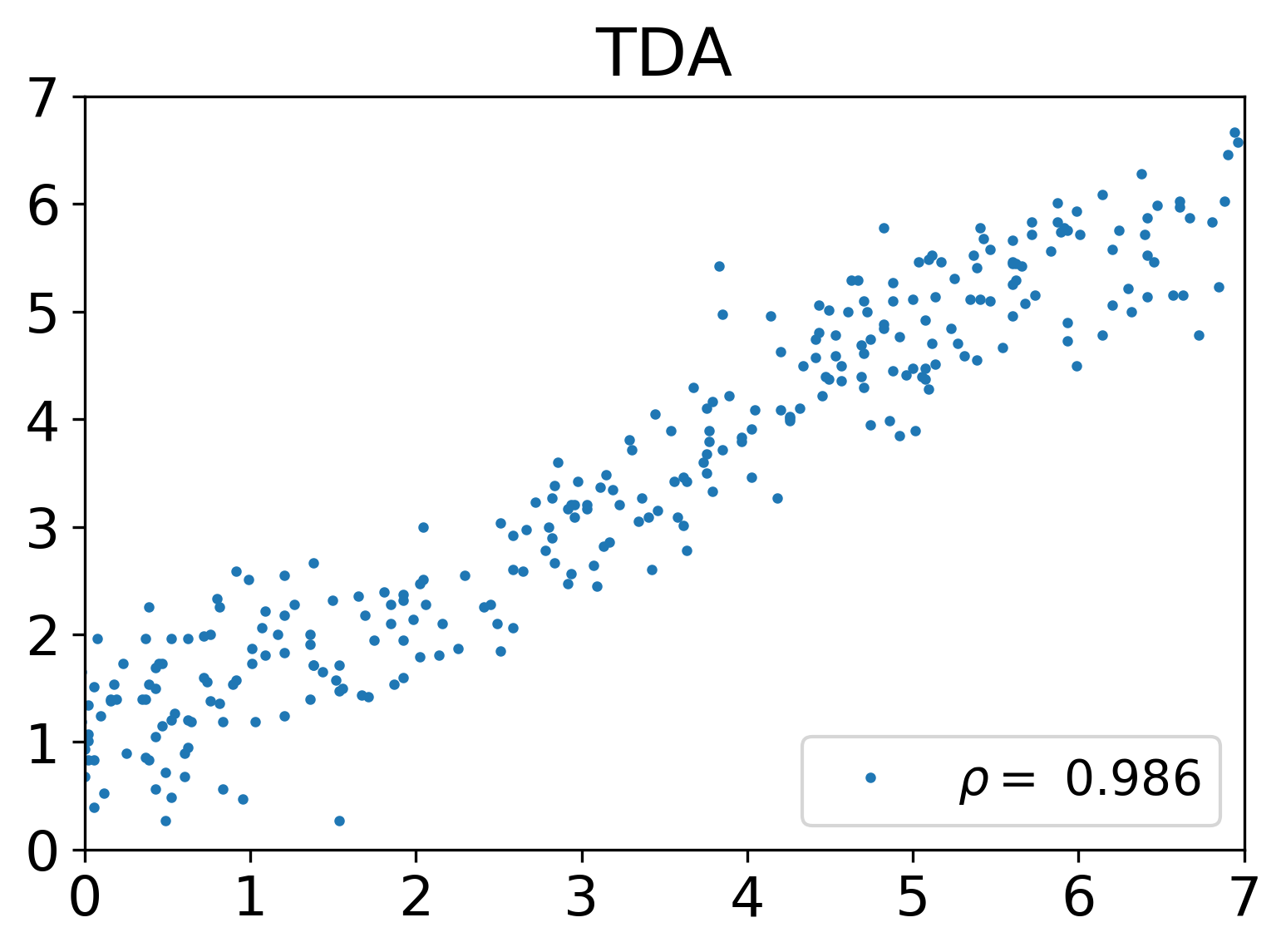
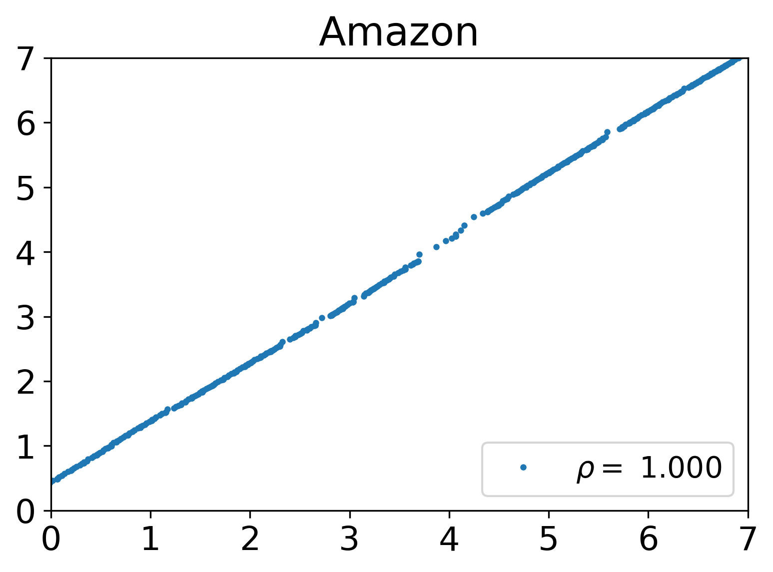
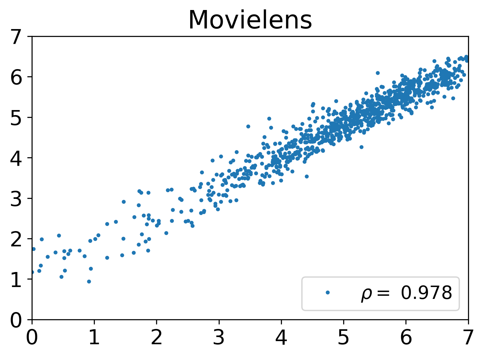
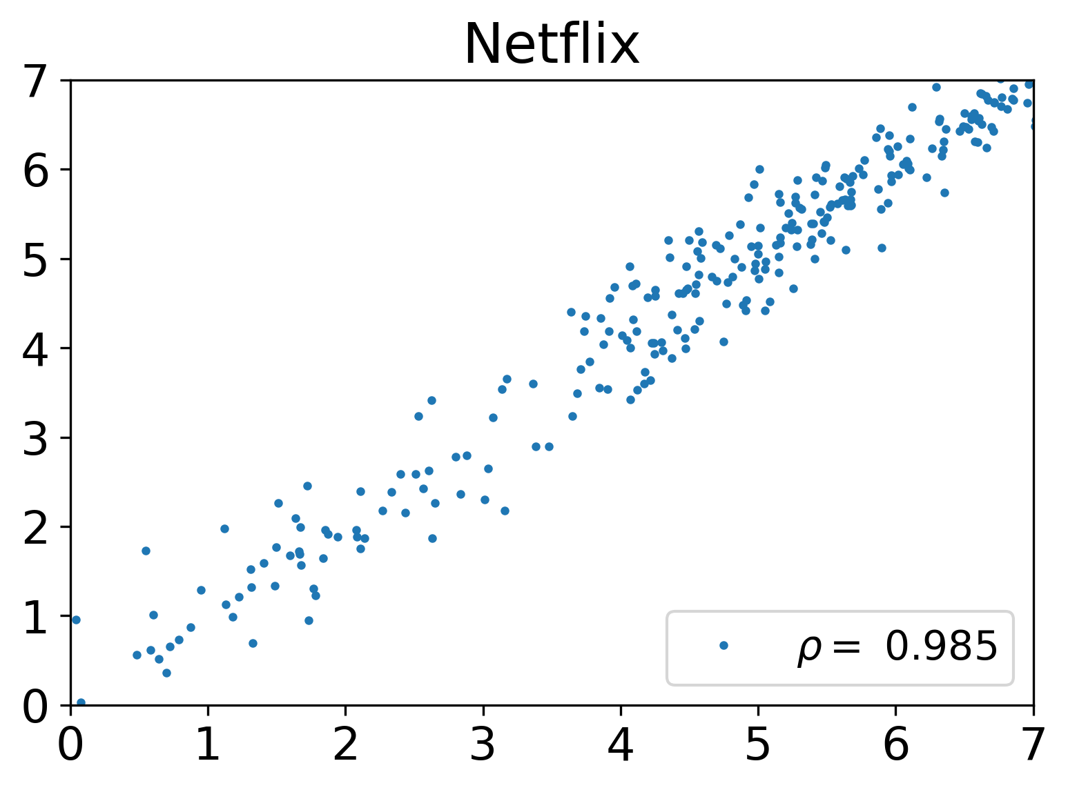
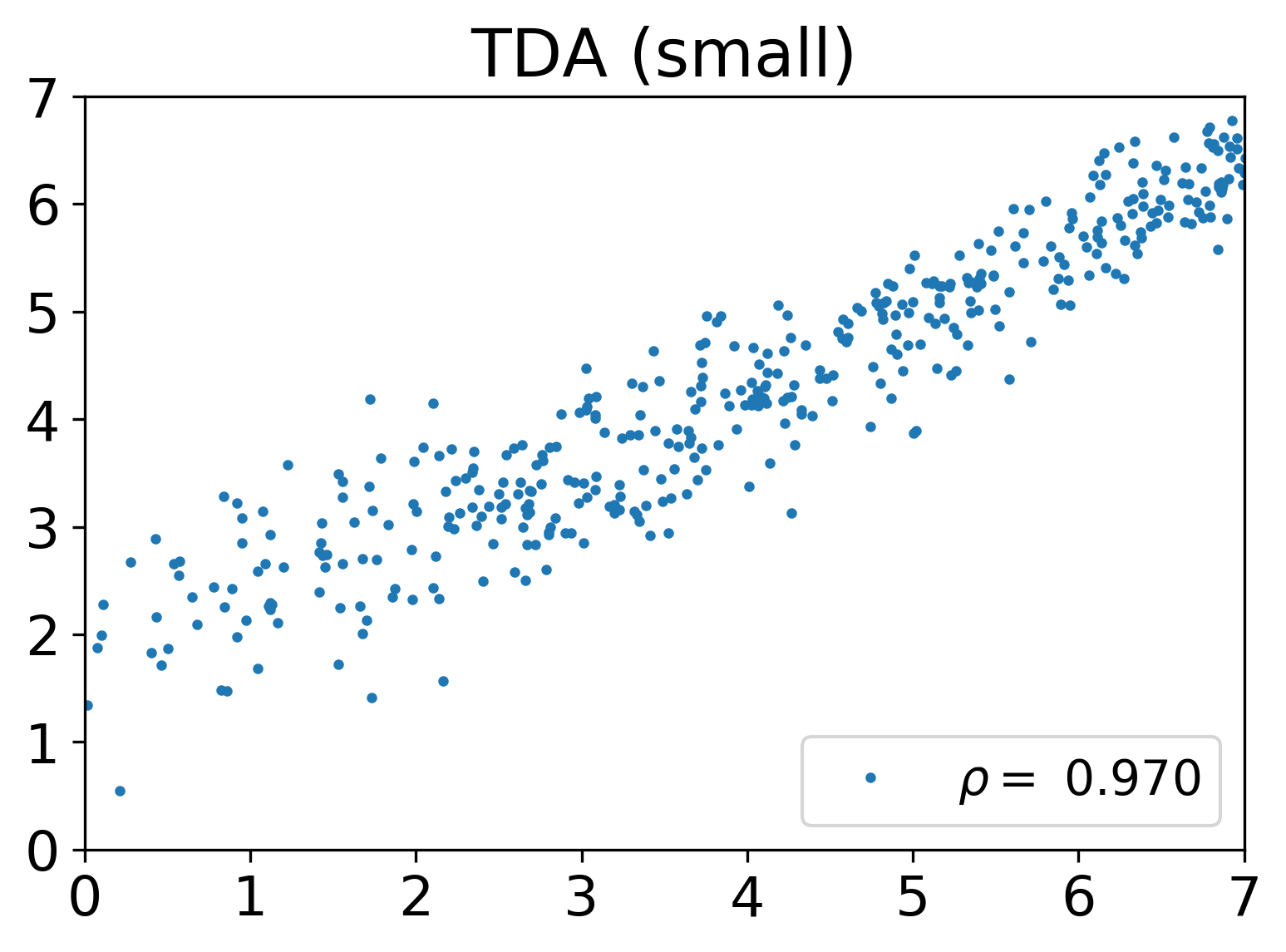
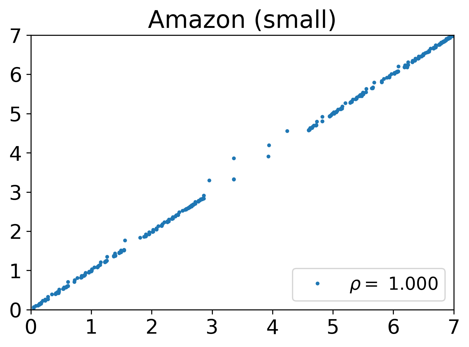
Figure 1: True vs. predicted log-likelihood on the test set (in arbitrary units).

Experiment I: Random accesses. In this experiment, an anomalous interval is simulated by adding random accesses to it: Each bit in the interval’s access matrix is changed to $1$ with an independent probability of $\epsilon>0$. We ran the algorithms 100 times on each data set, each time randomly selecting a single interval to simulate as anomalous. For each noise level, we calculated the AUC (Area under the curve) of the combined ROC curve, and plotted it against the value of $\log_{10}(\epsilon)$. The results of our algorithm and of MEAN on the full data sets, as well as the results of all algorithms on the down-sampled data sets, are reported in Figure 2. It can be seen that the regression model improved the identification of the anomaly in a wide range of noise levels, and that our algorithm is usually better than all baselines.

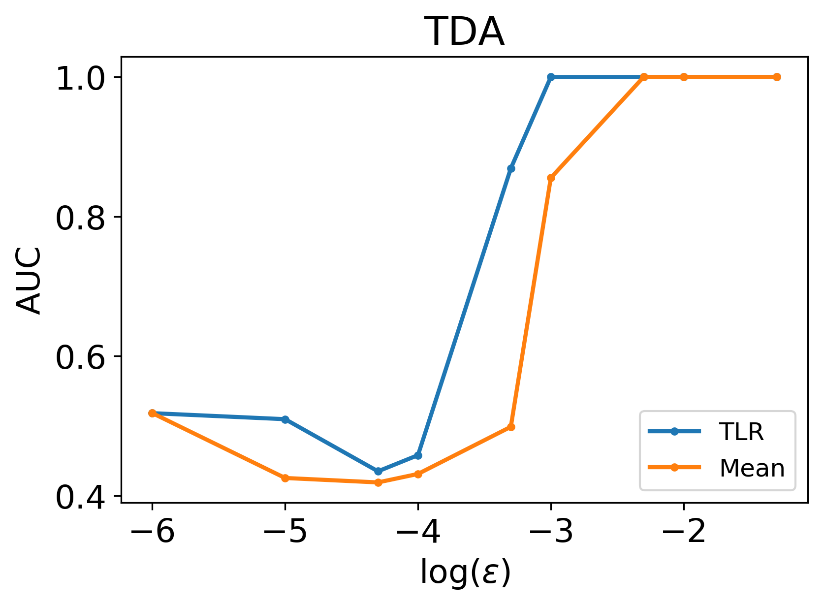
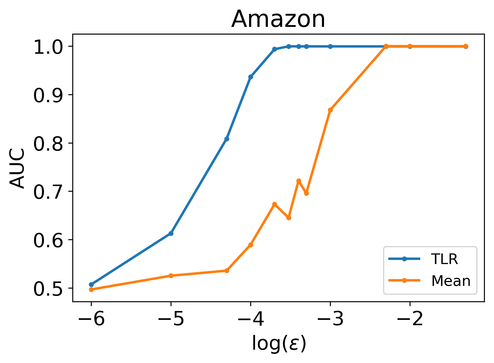
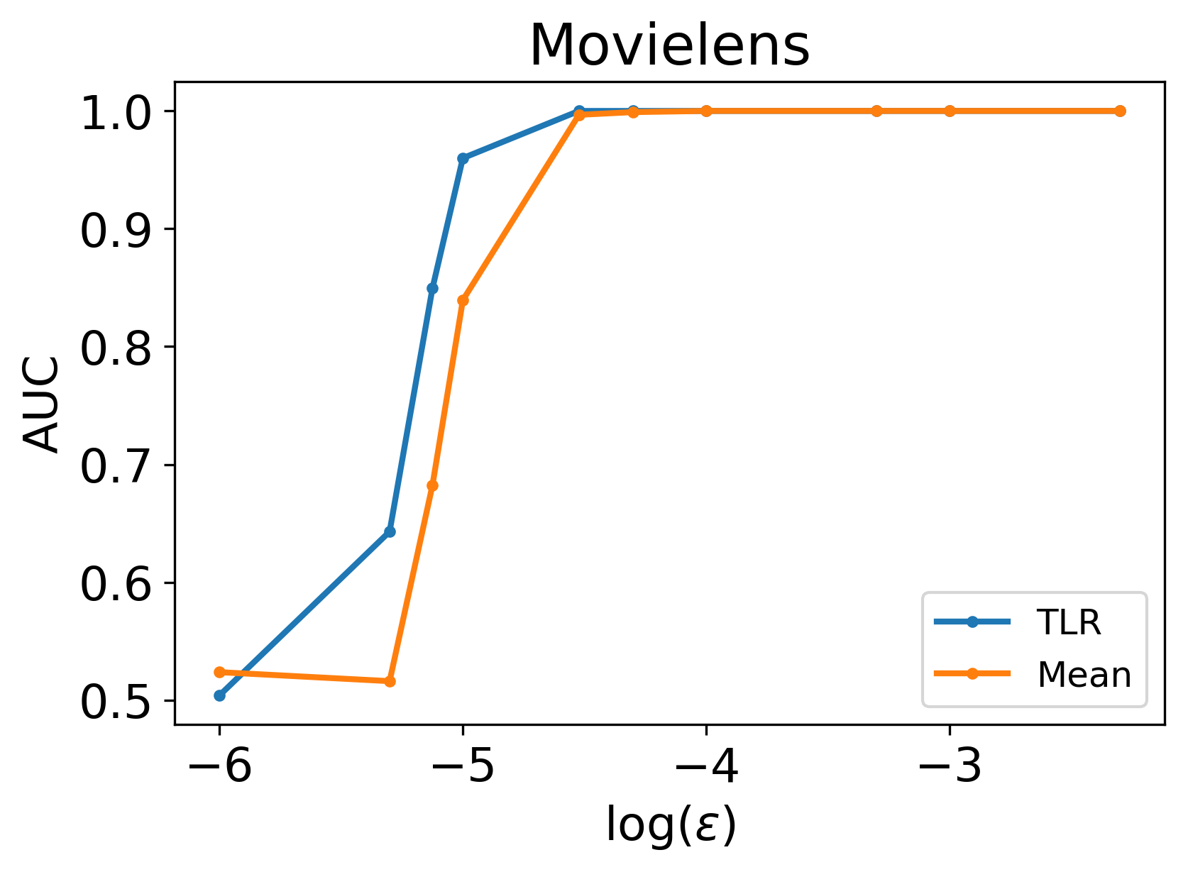
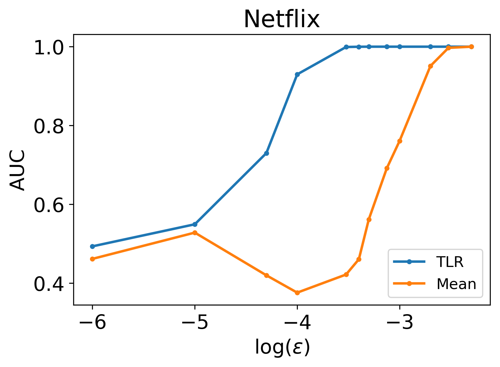
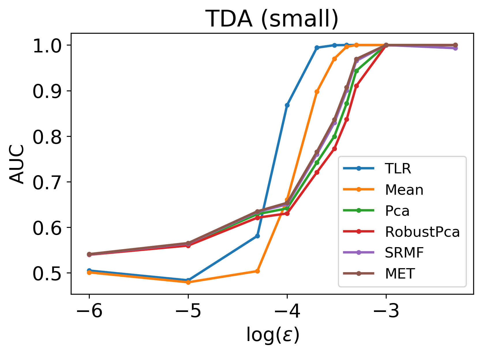
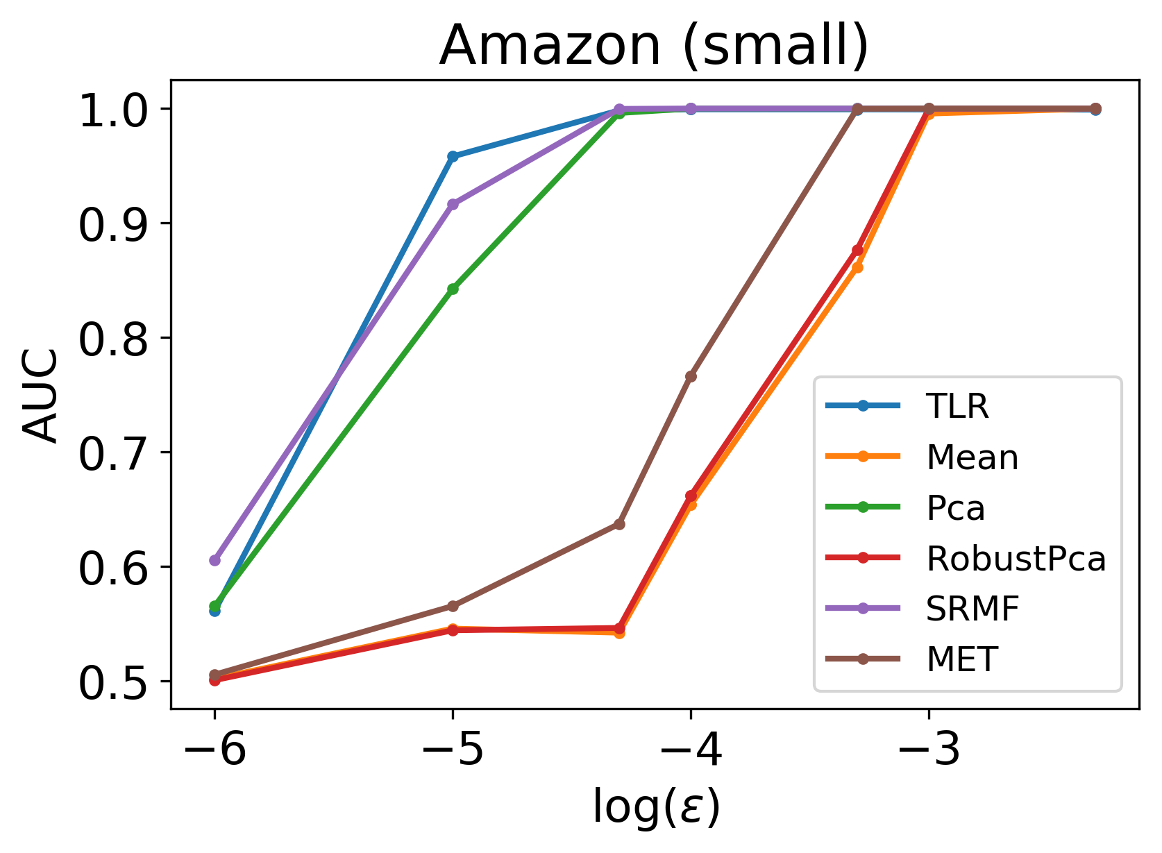
Figure 2: The AUC as a function of the log of the noise in the random access experiment.

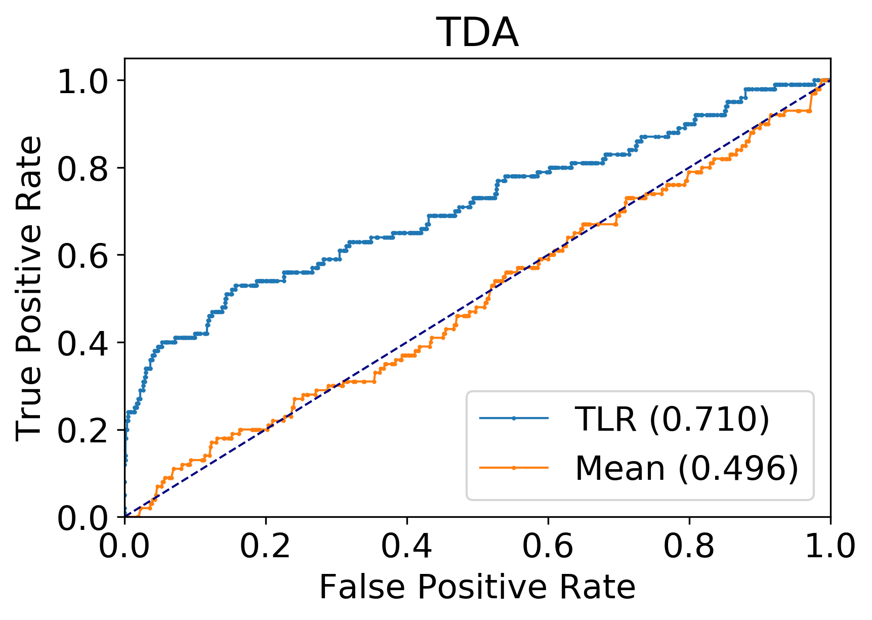
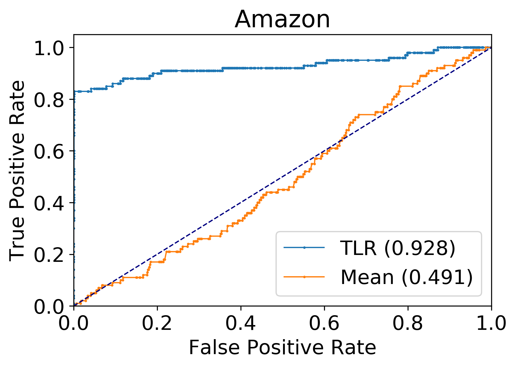
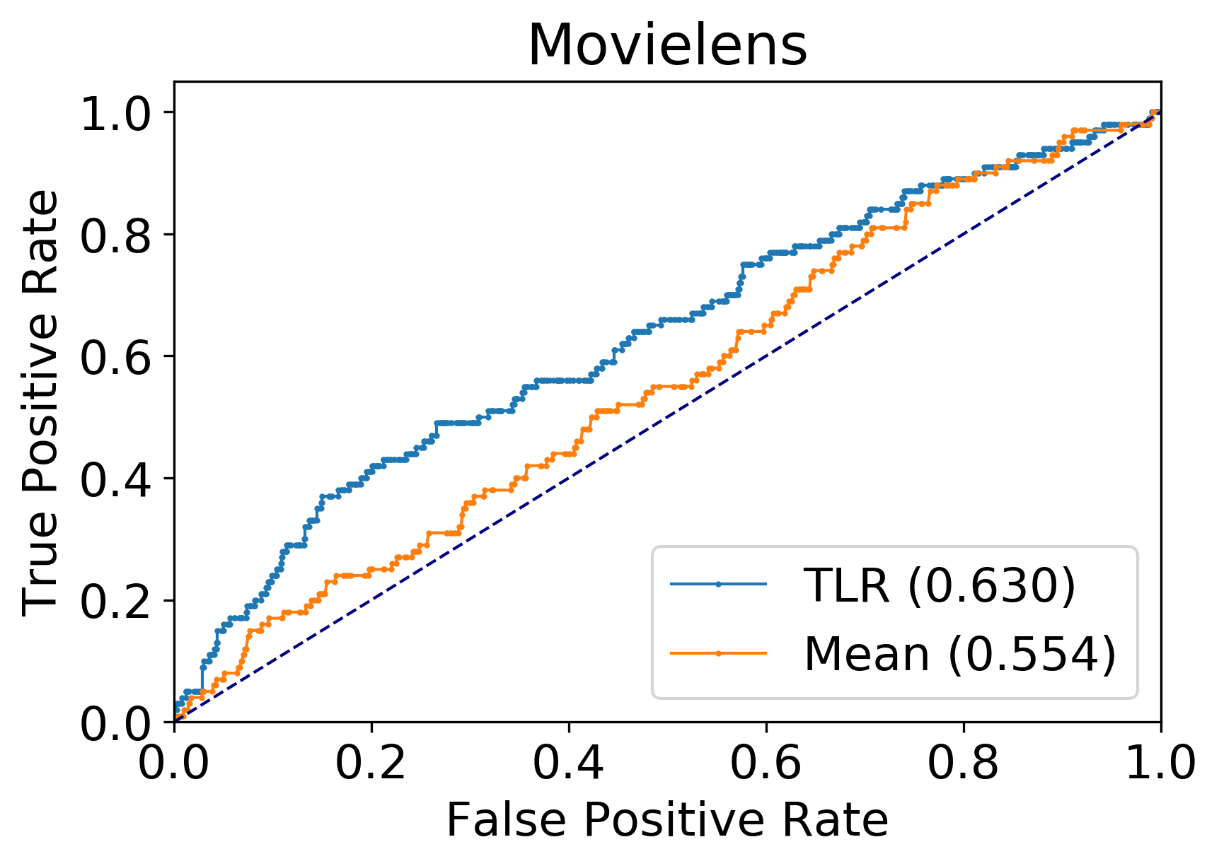
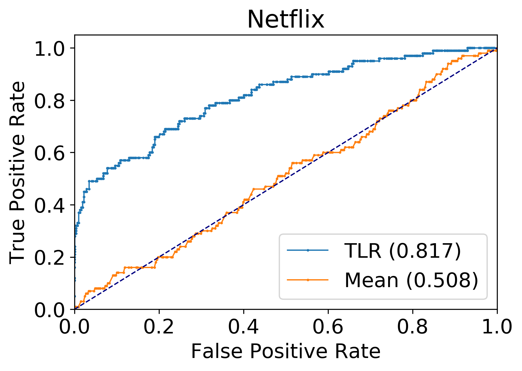
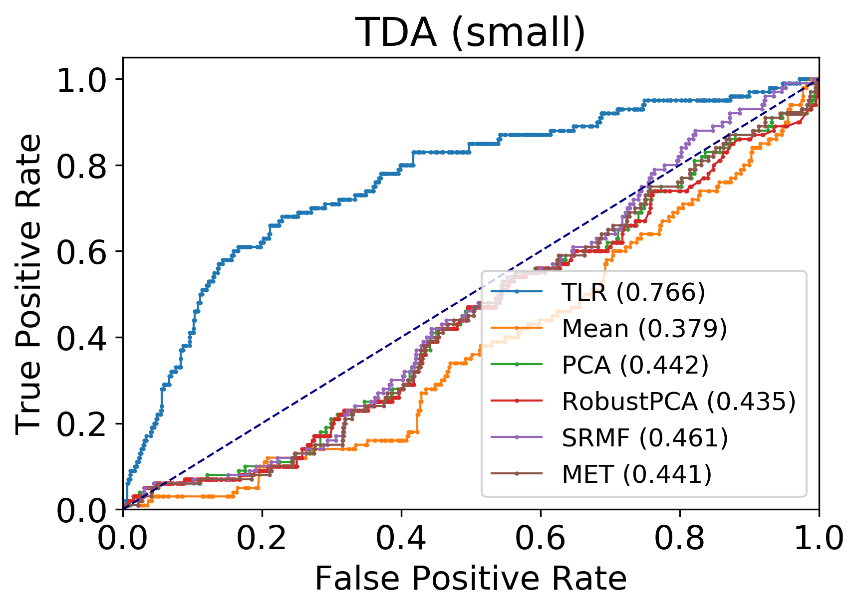
Figure 3: ROC curves for the anomalous time experiment. The AUC is given in parentheses.

Experiment II: Accesses at an anomalous time. We simulated a behavior which is normal at one time, but possibly anomalous at a different time, by replacing two randomly chosen intervals with each other. This moves intervals to a time in which they might be unexpected, hence should be identified as anomalies. We ran the algorithms 100 times on each data set, each time replacing intervals of a single random pair. Figure 3 shows the ROC curves generated from the anomaly scores of each of the algorithms. Note that if the times of the intervals in the pair are similar, e.g., both in the morning of a workday, then no anomaly should be identified. Thus, even the best algorithm could have an AUC which is not very close to one. Figure 3 shows that our algorithm is the most successful here. With the exception of SRMF, the other algorithms are not better than random guessing on this task. This should not be surprising, since these algorithms do not take into account the dependence on the timing of events.

Run time and memory

The baseline algorithms operate on a single matrix/tensor which includes the entire data set, and with no distinction between training time and test time. As a result, the memory requirements of these algorithms are prohibitive for large data sets. In contrast, our algorithm processes single-interval matrices one by one. Therefore, it requires significantly less memory. In addition, our algorithm performs matrix optimization only during training time, while the calculation of anomaly scores during test time is fast, and requires a small memory footprint for the trained model. This allows real-time anomaly detection as new matrices appear. Table 2 reports the run time of each of the algorithms on the tested data sets. The baseline algorithms could only be run on the reduced data sets due to their memory requirements. Our approach shows a clear run-time advantage, during training and more so during testing.

Data Set	TLR (train)	TLR (test)	SRMF	PCA	RobustPCA	MET
TDA	$\mathbf{946}$	$\mathbf{0.0029}$	-	-	-	-
Amazon	$\mathbf{16621}$	$\mathbf{0.0141}$	-	-	-	-
MovieLens	$\mathbf{4652}$	$\mathbf{0.0024}$	-	-	-	-
Netflix	$\mathbf{1964}$	$\mathbf{0.0071}$	-	-	-	-
TDA (small)	$\mathbf{45}$	$\mathbf{0.0042}$	229	140	338	50
Amazon (small)	$\mathbf{209}$	$\mathbf{0.0027}$	279	571	451	354

Table 2: Run-time (seconds) on an 2.8GHz Xeon CPU with 40 cores and 256 GB RAM.

6 Conclusions

The experiments demonstrate that our approach obtains superior results to previous algorithms, while requiring significantly less computational resources. While we focused here on identifying anomalous time intervals, this approach can be adapted to identifying specific users or objects which are anomalous. An additional important challenge is to develop a streaming version of the training stage. These adaptations will be studied in future work.

7 Acknowledgements

This work was supported in part by an IBM grant, and by the Israel Science Foundation (grants 555/15, 755/15).

Appendix A Appendix: Convergence analysis

For two real-valued matrices $X,Y\in\mathbb{R}^{n\times m}$, define the mean squared error between $X$ and $Y$ by

$$\mathrm{MSE}(X,Y):=\frac{1}{mn}\|X-Y\|_{F}^{2}.$$

Recall that ${\bar{\pi}}$ is the assumed stationary model, while $\hat{\pi}$ is our estimate of that stationary model. Below we show that by finding $F(\bar{B},\lambda)$, as defined in (3), we are effectively minimizing $\mathrm{MSE}(\hat{\pi},{\bar{\pi}})$ up to a term that decays to zero. (3) minimizes the squared Frobenius norm $\|\hat{\pi}-B\|_{F}^{2}$ with an additional regularization term $\lambda\|\hat{\pi}\|_{\mathrm{tr}}$. This is equivalent to minimizing $\|\hat{\pi}-B\|_{F}^{2}$ subject to a constraint on $\|\hat{\pi}\|_{\mathrm{tr}}$. Moreover, if $S=(B_{1},\ldots,B_{T})$ and $\bar{B}=\frac{1}{T}\sum_{t=1}^{T}B_{t}$, we have

$$\|\hat{\pi}-\bar{B}\|_{F}^{2}=\|\hat{\pi}\|_{F}^{2}-2\langle\hat{\pi},\bar{B}\rangle+\|\bar{B}\|_{F}^{2}=$$

$$\frac{1}{T}\sum_{t=1}^{T}\|\hat{\pi}-B_{t}\|_{F}^{2}-\frac{1}{T}\sum_{t=1}^{T}\|B_{t}\|_{F}^{2}+\|\bar{B}\|_{F}^{2}.$$

Therefore,

$$\|\hat{\pi}-\bar{B}\|_{F}^{2}=\frac{1}{T}\sum_{t=1}^{T}\|\hat{\pi}-B_{t}\|_{F}^{2}+C$$ (4)

$$=mn\cdot\frac{1}{T}\sum_{t=1}^{T}\mathrm{MSE}(\hat{\pi},B_{t})+C,$$ (5)

where $C$ is a constant independent of $\hat{\pi}$. By a similar derivation, for another constant $C^{\prime}$ independent of $\hat{\pi}$,

$$\mathbb{E}_{B\sim{\bar{\pi}}}[\mathrm{MSE}(\hat{\pi},B)]=\mathrm{MSE}(\hat{\pi},{\bar{\pi}})+C^{\prime}.$$

Therefore, if $|\mathbb{E}_{B\sim{\bar{\pi}}}[\mathrm{MSE}(\hat{\pi},B)]-\frac{1}{T}\sum_{t=1}^{T}\mathrm{MSE}(\hat{\pi},B_{t})|$ is small, finding $F(\bar{B},\lambda)$ is a good proxy for minimizing $\mathrm{MSE}(\hat{\pi},{\bar{\pi}})$. We prove a more general claim, which bounds the diffrence between the empirical loss and the true loss of a general Lipschitz loss, which we define below. Our result generalizes a result from (?) to the case of a training sample with several matrices. The proof employs techniques from (?) and (?).

Let $\ell:[0,1]\times[0,1]\rightarrow\mathbb{R}_{+}$ be a loss function. For two matrices $A,B\in[0,1]^{n\times m}$, let

$$\ell(A,B):=\frac{1}{nm}\sum_{i\in[n],j\in[m]}\ell(A(i,j),B(i,j)).$$

For $L>0$, $\ell$ is $L$-Lipschitz in the first argument if

$$\forall x,x^{\prime},y\in\mathbb{R},|\ell(x,y)-\ell(x^{\prime},y)|\leq L|x-x^{\prime}|,$$

with an analogous definition for the second argument.

For a matrix $X\in[0,1]^{n\times m}$ and a distribution $P$ over matrices $[0,1]^{n\times m}$; denote the true loss of $X$ by $\ell(X,P):=\mathbb{E}_{Y\in P}[\ell(X,Y)]$. For a (multi)set $S\subseteq[0,1]^{n\times m}$, denote the empirical loss of $X$ on $S$ by $\ell(X,S):=\frac{1}{|S|}\sum_{Y\in S}[\ell(X,Y)]$.

The theorem below gives a guarantee for $L$-Lipschitz losses. Note that for the squared-loss $\ell:=\mathrm{MSE}$, where $\mathrm{MSE}(x,y):=(x-y)^{2}$, $\ell$ is $2$-Lipschitz in both arguments: For $x,x^{\prime},y\in[0,1]$,

$$|(x-y)^{2}-(x^{\prime}-y)^{2}|=|x^{2}-x^{\prime 2}-2xy+2x^{\prime}y|$$

$$=|(x-x^{\prime})(x+x^{\prime})-2y(x-x^{\prime})|=|(x-x^{\prime})(x+x^{\prime}-2y)|$$

$$=|(x-x^{\prime})||(x+x^{\prime}-2y)|\leq 2|x-x^{\prime}|.$$

Thus the theorem below holds for the $\mathrm{MSE}$ loss with $L=2$, proving that as the size of the training set grows, minimizing (3) converges to a minimization of $\mathrm{MSE}(\hat{\pi},{\bar{\pi}})$ with high probability. In the following theorem and proof, we use $c$ to indicate a universal constant, whose value can change from line to line.

Theorem A.1.

Let $\ell(x,y)$ be an $L$-Lipschitz loss. Let ${\bar{\pi}}\in[0,1]^{n\times m}$, and let $\mathcal{D}_{\bar{\pi}}$ be the distribution satisfying the probabilistic model defined in Section 3. Assume w.l.o.g. that $m\geq n$. Let $S=(B_{1},B_{2},\ldots,B_{T})\sim\mathcal{D}_{\bar{\pi}}^{m}$ be an i.i.d. sample from $\mathcal{D}_{\bar{\pi}}$. With a probability of at least $1-\delta$, for all $\pi\in[0,1]^{n\times m}$ such that $\|\pi\|_{\mathrm{tr}}\leq\gamma$,

$$|\ell(\pi,\mathcal{D}_{{\bar{\pi}}})-\ell(\pi,S)|\leq c\frac{L\gamma}{n\sqrt{mT}}+L\sqrt{\frac{\ln(\frac{2}{\delta})}{2Tmn}}.$$

Proof.

Let $\Pi\subseteq[0,1]^{n\times m}$. Denote $\psi(S):=\sup_{\pi\in\Pi}(\ell(\pi,\mathcal{D}_{{\bar{\pi}}})-\ell(\pi,S))$. By definition,

$$\forall\pi\in\Pi,\quad\ell(\pi,\mathcal{D}_{{\bar{\pi}}})\leq\ell(\pi,S)+\psi(S).$$ (6)

Note that the sample $S$ has $Tnm$ independent (though not identically distributed) entries. Thus, we upper-bound $\psi(S)$ with high probability using McDiarmid’s inequality (?), which states that if for every two samples $S,S^{\prime}$ which differ by a single entry, $|\psi(S)-\psi(S^{\prime})|\leq\alpha$, then

$$\mathbb{P}\left[\psi(S)-\mathbb{E}[\psi(S)]\geq\epsilon\right]\leq e^{\frac{-2\epsilon^{2}}{Tnm\alpha^{2}}}.$$

To bound $\alpha$, consider two samples, $S,S^{\prime}$, where the matrices in $S$ are denoted $B_{t}$ and the matrices in $S^{\prime}$ are denoted $B^{\prime}_{t}$. Suppose that $S^{\prime}$ differs from $S$ by a single entry $(i,j)$ in the matrix $B_{t_{o}}$, such that $B_{t_{o}}(i,j)=1$ and $B^{\prime}_{t_{o}}(i,j)=0$. We have

$$|\psi(S)-\psi(S^{\prime})|=$$

$$|\sup_{\pi}(\ell(\pi,\mathcal{D}_{{\bar{\pi}}})-\ell(\pi,S))-\sup_{\pi}(\ell(\pi,\mathcal{D}_{{\bar{\pi}}})-\ell(\pi,S^{\prime}))|$$

For bounded $f,g:\mathbb{R}\rightarrow\mathbb{R}$, it holds that $|\sup_{x}f(x)-\sup_{x}g(x)|\leq|\sup_{x}(f(x)-g(x))|$. Therefore

$$|\psi(S)-\psi(S^{\prime})|\leq\frac{1}{T}|\sup_{\pi}\sum_{t}(\ell(\pi,B_{t})-\ell(\pi,B^{\prime}_{t}))|$$

$$=\frac{1}{Tmn}|\sup_{\pi}(\ell(\pi(i,j),B_{t_{o}}(i,j))-\ell(\pi(i,j),B^{\prime}_{t_{o}}(i,j))|$$

$$\leq\frac{L}{Tmn}|B_{t_{o}}(i,j)-B^{\prime}_{t_{o}}(i,j)]|\leq\frac{L}{Tmn},$$

Where we used the fact that $\ell$ is $L$-Lipschitz in the second argument. Setting $\alpha=L/(Tnm)$ and applying McDiarmid’s inequality, we get

$$\mathbb{P}[\psi(S)-\mathbb{E}[\psi(S)]\geq\epsilon]\leq e^{-2\epsilon^{2}Tmn/L^{2}}.$$

Setting the latter to $\frac{\delta}{2}$, we obtain that with a probability of at least $1-\frac{\delta}{2}$,

$$\psi(S)\leq\mathbb{E}[\psi(S)]+L\sqrt{\frac{\ln(\frac{2}{\delta})}{2Tmn}}.$$ (7)

It remains to bound $\mathbb{E}[\psi(S)]$. Let $S^{\prime}=(B^{\prime}_{1},\ldots,B^{\prime}_{T})\sim\mathcal{D}_{\bar{\pi}}^{T}$ be a sample which is independent from $S$. Following a standard symmetrization argument as in (?), we have

$$\mathbb{E}[\psi(S)]=\mathbb{E}_{S}[\sup_{\pi}(\ell(\pi,\mathcal{D}_{{\bar{\pi}}})-\ell(\pi,S))]]$$

$$=\mathbb{E}_{S}[\sup_{\pi}(\mathbb{E}_{S^{\prime}}[\ell(\pi,S^{\prime})-\ell(\pi,S)])]$$

$$\leq\mathbb{E}_{S,S^{\prime}}[\sup_{\pi}(\ell(\pi,S^{\prime})-\ell(\pi,S))]$$

$$=\frac{1}{mnT}\mathbb{E}_{S,S^{\prime}}\big{[}\sup_{\pi}\sum_{i,j,t}\ell(\pi(i,j),B^{\prime}_{t}(i,j))$$

$$\qquad\qquad-\ell(\pi(i,j),B_{t}(i,j))\big{]}.$$

Letting $\sigma_{i,j,t}\sim\mathrm{Uniform}\{-1,1\}$ for $i\in[n],j\in[m],t\in[T]$ be independent Rademacher variables, it follows that

$$\mathbb{E}[\psi(S)]=$$

$$\frac{1}{mnT}\mathbb{E}_{S,S^{\prime},\sigma}\Big{[}\sup_{\pi}\sum_{i,j,t}\sigma_{i,j,t}\big{(}\ell(\pi(i,j),B^{\prime}_{t}(i,j))$$

$$\qquad\qquad\qquad-\ell(\pi(i,j),B_{t}(i,j))\big{)}\Big{]}$$ (8)

$$\leq\frac{2}{mnT}\mathbb{E}_{S,\sigma}\left[\sup_{\pi}\sum_{i,j,t}\sigma_{i,j,t}\ell(\pi(i,j),B_{t}(i,j))\right]$$

$$\leq\frac{2L}{mnT}\mathbb{E}_{\sigma}\left[\sup_{\pi(i,j)}\sum_{i,j,t}\sigma_{i,j,t}\pi(i,j).\right]$$ (9)

The last inequality follows from Talagrand’s contraction principle (?), together with the fact that $\ell(x,y)$ is $L$-Lipschitz in both arguments.

Now, denoting $\nu_{i,j}:=\sum_{t}\sigma_{i,j,t}$, we observe that

$$\mathbb{E}_{\sigma}\left[\sup_{\pi}\sum_{i,j,t}\sigma_{i,j,t}\pi(i,j)\right]=$$

$$\mathbb{E}_{\sigma}\left[\sup_{\pi}\sum_{i,j}\pi(i,j)\sum_{t}\sigma_{i,j,t}\right]=\mathbb{E}_{\sigma}\left[\sup_{\pi}\sum_{i,j}\pi(i,j)\nu_{i,j}\right]$$

Since the nuclear and spectral norms are dual (?), a matrix Hölder inequality holds, where $\nu$ is the matrix with entries $\nu_{i,j}$:

$$\sum_{i,j}\pi(i,j)\nu_{i,j}\leq\|\pi\|_{\mathrm{tr}}\|\nu\|_{{}_{\mathrm{sp}}}.$$

Therefore, combining with (9), and assuming $\sup_{\pi\in\Pi}\|\pi\|_{\mathrm{tr}}\leq\gamma$, it follows that

$$\mathbb{E}[\psi(S)]\leq\frac{2L}{mnT}\mathbb{E}_{\sigma}[\sup_{\pi\in\Pi}\|\pi\|_{\mathrm{tr}}\|\nu\|_{{}_{\mathrm{sp}}}]\leq\frac{2L\gamma}{mnT}\mathbb{E}_{\sigma}[\|\nu\|_{{}_{\mathrm{sp}}}].$$ (10)

It remains to bound $\mathbb{E}_{\sigma}\left[||\nu||_{{}_{\mathrm{sp}}}\right]$. To this end, recall the following result of ? (?): There is a universal constant $c>0$ such that for any random matrix $Z\in\mathbb{R}^{n\times m}$ with independent mean-zero entries, we have

$$\mathbb{E}\left[||Z||_{{}_{\mathrm{sp}}}\right]\leq$$

$$c\Big{(}\max_{i}\sqrt{\sum_{j}\mathbb{E}\left[Z(i,j)^{2}\right]}$$

$$\qquad+\max_{j}\sqrt{\sum_{i}\mathbb{E}\left[Z(i,j)^{2}\right]}+\sqrt[4]{\mathbb{E}\left[Z(i,j)^{4}\right]}\Big{)}.$$

Now $\nu_{i,j}$ is a sum of $T$ i.i.d. Rademacher random variables, and thus $\mathbb{E}[\nu_{i,j}]=0$ and $\mathbb{E}[\nu_{i,j}^{2}]=T$. To bound the $4$th moment, we appeal to Khinchine’s inequality (?, Exercise 5.10), which states that $\mathbb{E}[\nu_{i,j}^{4}]\leq\frac{4!}{2\cdot 2^{2}}\mathbb{E}[\nu_{i,j}^{2}]^{2}=3T^{2}.$ Substituting these moment bounds into Latała’s bound, we get

$$\mathbb{E}\left[||\nu||_{{}_{\mathrm{sp}}}\right]\leq c\left(\sqrt{nT}+\sqrt{mT}+\sqrt[4]{nm}\sqrt{T}\right).$$

Since $\sqrt[4]{nm}\leq\frac{1}{2}(\sqrt{n}+\sqrt{m})$ and $m\geq n$, we have $\mathbb{E}\left[||\nu||_{{}_{\mathrm{sp}}}\right]\leq c\sqrt{Tm}$. Substituting this into (10), we get

$$\mathbb{E}[\psi(S)]\leq c\frac{L\gamma}{n\sqrt{mT}}.$$

Combining this with (7) yields that with probability of at least $1-\frac{\delta}{2}$,

$$\psi(S)\leq c\frac{L\gamma}{n\sqrt{mT}}+L\sqrt{\frac{\ln(\frac{2}{\delta})}{2Tmn}}.$$

Combining this with (6) and the observation that

$$\forall\pi\in\Pi~{}~{}\ell(\pi,\mathcal{D}_{\pi})$$ (11)

$$\leq\ell(\pi,S)+\sup_{\pi^{\prime}\in\Pi}(\ell(\pi^{\prime},\mathcal{D}_{\pi})-\ell(\pi^{\prime},S))$$ (12)

$$\leq\ell(\pi,S)+\psi(S)$$ (13)

, we get that if $\sup_{\pi\in\Pi}\|\pi\|_{\mathrm{tr}}\leq\gamma$, then with probability of at least $1-\frac{\delta}{2}$,

$$\forall\pi\in\Pi,\quad\ell(\pi,\mathcal{D}_{{\bar{\pi}}})-\ell(\pi,S)\leq c\frac{L\gamma}{n\sqrt{mT}}+L\sqrt{\frac{\ln(\frac{2}{\delta})}{2Tmn}}.$$

An analogous argument yields the same bound for $\ell(\pi,S)-\ell(\pi,\mathcal{D}_{\bar{\pi}})$, which implies the statement of the theorem via a union bound. ∎

References

- [2007] T. Ahmed; M. Coates; A. Lakhina. 2007. Multivariate online anomaly detection using kernel recursive least squares. INFOCOM.
- [2007] Bennett, J.; Lanning, S.; et al. 2007. The netflix prize. In Proceedings of KDD cup and workshop, volume 2007, 35.
- [2013] Boucheron, S.; Lugosi, G.; and Massart, P. 2013. Concentration inequalities: A nonasymptotic theory of independence.
- [2011] Candès, E. J.; Li, X.; Ma, Y.; and Wright, J. 2011. Robust principal component analysis? J. ACM 58(3):11:1–11:37.
- [2003] Chan, P. K.; Mahoney, M. V.; and Arshad, M. H. 2003. A machine learning approach to anomaly detection. Florida Inst. Tech.
- [1999] Chung, C. Y.; Gertz, M.; and Levitt, K. 1999. DEMIDS: A misuse detection system for database systems.
- [2007] Das, K., and Schneider, J. 2007. Detecting anomalous records in categorical datasets. SIGKDD
- [2008] Das, K.; Schneider, J.; and Neill, D. B. 2008. Anomaly pattern detection in categorical datasets. SIGKDD
- [2014] Davenport, M. A.; Plan, Y.; van den Berg, E.; Wootters, M. 2014. 1-bit matrix completion. Information and Inference.
- [1990] Deerwester, S.; Dumais, S. T.; Furnas, G. W.; Landauer, T. K.; and Harshman, R. 1990. Indexing by latent semantic analysis. Journal of the American society for information science 41(6):391.
- [2002] Fazel, M. 2002. Matrix rank minimization with applications. Ph.D. Dissertation, PhD thesis, Stanford University.
- [2015] Görnitz, N.; Braun, M. L.; and Kloft, M. 2015. Hidden markov anomaly detection. ICML.
- [2014] Günnemann, S.; Günnemann, N.; and Faloutsos, C. 2014. Detecting anomalies in dynamic rating data: A robust probabilistic model for rating evolution. SIGKDD
- [2016] Harper, F. M., Konstan, J. A. 2016. The movielens datasets: History and context. ACM TIIS.
- [2010] Höhle, M. 2010. Online change-point detection in categorical time series. In Statistical modelling and regression structures.
- [2013] Horn, R. A., and Johnson, C. R. 2013. Matrix analysis. Cambridge University Press, Cambridge, second edition.
- [2015] Hsieh, C.-J.; Natarajan, N.; and Dhillon, I. S. 2015. Pu learning for matrix completion. In ICML, 2445–2453.
- [2008] Kamra, A.; Terzi, E.; and Bertino, E. 2008. Detecting anomalous access patterns in relational databases. VLDB J 17(5):1063–1077.
- [2014] Khaleghi, A., and Ryabko, D. 2014. Asymptotically consistent estimation of the number of change points in highly dependent time series. In ICML, 539–547.
- [2008] Kolda, T. G., and Sun, J. 2008. Scalable tensor decompositions for multi-aspect data mining. ICDM.
- [2004] Lakhina, A.; Crovella, M.; and Diot, C. 2004. Diagnosing network-wide traffic anomalies. SIGCOMM.
- [2000] Larsen, R. M. 2000. Computing the svd for large and sparse matrices. SCCM, Stanford University, June 16.
- [2005] Latała, R. 2005. Some estimates of norms of random matrices. Proc. AMS 133(5):1273–1282.
- [1991] Ledoux, M., and Talagrand, M. 1991. Probability in Banach Spaces. Springer-Verlag.
- [2002] Lee, S. Y.; Low, W. L.; and Wong, P. Y. 2002. ESORICS.
- [2014] Leskovec, J.; Rajaraman, A.; and Ullman, J. D. 2014. Mining of massive datasets. Cambridge University Press.
- [2017] Levi, M.; Allouche, Y.; and Kontorovich, A. 2018. Advanced analytics for connected cars cyber security. In 87th IEEE Vehicular Technology Conference, VTC Spring 2018.
- [2013] Lichman, M. 2013. UCI machine learning repository.
- [1999] Manning, C. D., and Schütze, H. 1999. Foundations of statistical natural language processing. MIT Press, Cambridge, MA.
- [2010] Mathew, S.; Petropoulos, M.; Ngo, H. Q.; and Upadhyaya, S. J. 2010. A data-centric approach to insider attack detection in database systems. RAID.
- [2010] Mazumder, R.; Hastie, T.; and Tibshirani, R. 2010. Spectral regularization algorithms for learning large incomplete matrices. Journal of machine learning research 11(Aug):2287–2322.
- [1989] McDiarmid, C. 1989. On the method of bounded differences. Surveys in combinatorics 141(1):148–188.
- [2010] Rendle, S. 2010. Factorization machines. In 2010 IEEE International Conference on Data Mining, 995–1000.
- [2012] Roughan, M.; Zhang, Y.; Willinger, W.; and Qiu, L. 2012. Spatio-temporal compressive sensing and internet traffic matrices. IEEE/ACM Trans. Netw..
- [2014] Santos, R. J.; Bernardino, J.; and Vieira, M. 2014. Approaches and challenges in database intrusion detection. SIGMOD Record 43(3):36–47.
- [2014] Shamir, O., and Shalev-Shwartz, S. 2014. Matrix completion with the trace norm: learning, bounding, and transducing. Journal of Machine Learning Research 15(1):3401–3423.
- [1995] Shardanand, U., and Maes, P. 1995. Social information filtering: algorithms for automating ”word of mouth”. SIGCHI.
- [2010] Sindhwani, V.; Bucak, S. S.; Hu, J.; and Mojsilovic, A. 2010. One-class matrix completion with low-density factorizations. ICMD.
- [2005] Soule, A.; Salamatian, K.; Nucci, A.; and Taft, N. 2005. Traffic matrix tracking using kalman filters. SIGMETRICS Perform. Eval. Rev. 33(3):24–31.
- [2005] Spalka, A., and Lehnhardt, J. 2005. A comprehensive approach to anomaly detection in relational databases. Data and Applications Security.
- [2004] Srebro, N.; Alon, N.; and Jaakkola, T. S. 2004. Generalization error bounds for collaborative prediction with low-rank matrices. NIPS.
- [2006] Srivastava, A.; Sural, S.; and Majumdar, A. K. 2006. Database intrusion detection using weighted sequence mining. JCP 1(4):8–17.
- [2009] Su, X., and Khoshgoftaar, T. M. 2009. A survey of collaborative filtering techniques. Advances in artificial intelligence.
- [2006] Takeuchi, J.-i., and Yamanishi, K. 2006. A unifying framework for detecting outliers and change points from time series. IEEE Trans. Knowl. Data Eng.
- [2006] Tartakovsky, A. G.; Rozovskii, B. L.; Blazek, R. B.; and Kim, H. 2006. A novel approach to detection of intrusions in computer networks via adaptive sequential and batch-sequential change-point detection methods. IEEE Trans. Sig. Proc. 54(9):3372–3382.
- [2017] Zhou, C. and Paffenroth, R. C. 2017. Anomaly detection with robust deep autoencoders. SIGKDD, 665–674.
- [2017] Azzouni, A. and Pujolle, G. 2017. A long short-term memory recurrent neural network framework for network traffic matrix prediction. arXiv:1705.05690.