An extensive VLT/X-Shooter library of photospheric templates
of pre-main sequence stars

Abstract

Context. Studies of the formation and evolution of young stars and their disks rely on knowledge of the stellar parameters of the young stars. The derivation of these parameters is commonly based on comparison with photospheric template spectra. Furthermore, chromospheric emission in young active stars impacts the measurement of mass accretion rates, a key quantity for studying disk evolution.

Aims. Here we derive stellar properties of low-mass ($M_{\star}$$\lesssim$ 2 $M_{\odot}$) pre-main sequence stars without disks, which represent ideal photospheric templates for studies of young stars. We also use these spectra to constrain the impact of chromospheric emission on the measurements of mass accretion rates. The spectra are reduced, flux-calibrated, and corrected for telluric absorption, and are made available to the community.

Methods. We derive the spectral type for our targets by analyzing the photospheric molecular features present in their VLT/X-Shooter spectra by means of spectral indices and comparison of the relative strength of photospheric absorption features. We also measure effective temperature, gravity, projected rotational velocity, and radial velocity from our spectra by fitting them with synthetic spectra with the ROTFIT tool. The targets have negligible extinction ($A_{V}<0.5$ mag) and spectral type from G5 to K6, and from M6.5 to M8. They thus complement the library of photospheric templates presented by Manara et al. (2013a). We perform synthetic photometry on the spectra to derive the typical colors of young stars in different filters. We measure the luminosity of the emission lines present in the spectra and estimate the noise due to chromospheric emission in the measurements of accretion luminosity in accreting stars.

Results. We provide a calibration of the photospheric colors of young pre-main sequence stars as a function of their spectral type in a set of standard broad-band optical and near-infrared filters. The logarithm of the noise on the accretion luminosity normalized to the stellar luminosity is roughly constant and equal to $\sim-$2.3 for targets with masses larger than 1 solar mass, and decreases with decreasing temperatures for lower-mass stars. For stars with masses of $\sim 1.5M_{\odot}$ and ages of $\sim$1-5 Myr, the chromospheric noise converts to a limit of measurable mass accretion rates of $\sim 3\cdot 10^{-10}M_{\odot}$/yr. The limit on the mass accretion rate set by the chromospheric noise is of the order of the lowest measured values of mass accretion rates in Class II objects.

1 Introduction

The phase of pre-main sequence (PMS) stellar evolution is key for the final stellar mass build-up and for the evolution and dispersal of the surrounding circumstellar disks (e.g., Hartmann et al., 2016). This, in turn, has a strong impact on the final architecture of the planetary systems that form in the disk (Morbidelli & Raymond, 2016).

The determination of how the star accretes mass from the disk, how the system loses mass through winds, and how these processes affect disk evolution, requires a good knowledge of the properties of the central star. In particular, one needs to know its effective temperature ($T_{\rm eff}$) and luminosity ($L_{\star}$), and also the surface gravity (log$g$) and projected rotation velocity ($v$sin$i$), which are the main parameters shaping its photospheric emission flux. This photospheric flux must be subtracted from the observed spectrum in order to measure accretion and ejection diagnostics. The best approach seems to be to use as photospheric templates the spectra of disk-less non-accreting pre-main sequence stars, known as Class III objects based on their infrared classification, as they have similar surface gravity (intermediate between giants and dwarfs) to the accreting stars (Class II objects). Current synthetic spectra for such low-surface-gravity objects are not entirely reliable, as they do not fully reproduce medium- or high-resolution spectra of low-gravity objects (e.g., Allard et al., 2011). On the other hand, synthetic spectra are still valuable templates of non-active stars, and are therefore needed to evaluate the chromosperic flux emitted by very young stars. Therefore, spectra of Class III objects are needed both as photospheric templates and to further calibrate synthetic spectra.

In Manara et al. (2013a, hereafter MTR13) we presented flux-calibrated spectra of 24 low-mass non-accreting PMS stars covering a large wavelength range ($\lambda\lambda\sim$ 300 - 2500 nm), obtained with the medium-resolution spectrograph VLT/X-Shooter. This sample included objects with spectral type from K5 to M9.5 with typically two or more objects per spectral sub-class. The spectra, fully reduced and calibrated, were made available to the community and have already been used as templates for several studies (e.g., Alcalá et al., 2014, 2017; Banzatti et al., 2014; Fang et al., 2016; Manara et al., 2015, 2016, 2017; Manjavacas et al., 2014; Stelzer et al., 2013b; Whelan et al., 2014). From the same spectra we estimated the contribution of chromospheric activity to the emission lines typically used to estimate the accretion luminosity of accreting stars, showing that this has a strong dependence on the spectral type, and hence the stellar mass, of the target. A more detailed study of the photospheric and chromospheric properties of these stars, in particular their effective temperature, surface gravity, rotational velocity, and radial velocity, as well as the comparison between chromospheric and coronal emissions, was then carried out by Stelzer et al. (2013a). This work showed that the chromospheric emission saturates for early-M stars and that the coronal flux dominates that of the chromosphere.

Here we extend the library of photospheric templates with spectra of 16 additional non-accreting PMS stars presented here for the first time and one previously analyzed object. These additional objects have spectral types from G5 to M8, in particular in the ranges not covered by MTR13. The total sample of 41 reduced spectra, including one already analyzed in Manara et al. (2016), is made available through the Centre de Données astronomiques de Strasbourg (CDS) . We present the sample selection, observations, and data reduction in Sect. 2. Then, we discuss the analysis of the spectra and the photospheric properties of these objects in Sect. 3. In Sect. 5 we analyze the emission lines present in the spectra and the implications for measurements of mass accretion rates in PMS objects with disks. Finally, we perform synthetic photometry on the spectra and derive the typical colors for PMS stars in Sect. 4.

2 Sample, observations, and data reduction

The targets were selected to be bona-fide young stellar objects without a disk, that is, Class III according to classifications based on Spitzer data (e.g., Evans et al., 2009), and with negligible or very low extinction, that is, $A_{V}\lesssim$0.5 mag. Moreover, we searched for objects classified in the literature to have spectral type in the G and early K spectral classes, or in the late M spectral class, in order to cover the gaps in spectral types of the library of photospheric templates of young stars studied by MTR13 and Stelzer et al. (2013a). We based our selection on the works of Wahhaj et al. (2010), Manoj et al. (2011), Luhman (2007), and Luhman et al. (2008) and selected 16 single stars for observations. The objects are located in the Taurus, Chamaleon I, Lupus, and Upper Scorpius star-forming regions. Coordinates, information from the literature and archival photometry for these targets are reported in Tables 7-8 of the Appendix A. Information on the binarity of the targets was searched for in the literature (e.g., Nguyen et al., 2012; Daemgen et al., 2015) and is reported in Table 7.

Observations were carried out with the ESO VLT/X-Shooter spectrograph (Vernet et al., 2011). This spectrograph covers simultaneously the wavelength range from $\sim$300 nm to $\sim$2500 nm, and the spectra are divided into three arms, the UVB ($\lambda\lambda\sim$ 300-550 nm), the VIS ($\lambda\lambda\sim$ 500-1050 nm), and the NIR ($\lambda\lambda\sim$ 1000-2500 nm). Slits with different widths were used in the three arms and for brighter or fainter targets. The brighter earlier-type objects were observed with the narrower slits (0.5″-0.4″-0.4″ in the three arms, respectively) leading to the highest spectral resolution (R$\sim$9900, 18200, 10500 in the three arms, respectively). The targets with later spectral type were instead observed using larger slits (1.3″-0.9″-0.9″) leading to lower spectral resolution (R$\sim$ 4000, 7450, 5300) but also to lower flux losses. All the targets were also observed with wider slits of 5.0″ prior to the narrow slit observations to obtain a spectrum with no flux losses needed for absolute flux calibration. The log of the observations is reported in Table 9. The S/N of the spectra depends on the wavelength and on the brightness of the targets. The targets with G- and K-spectral types (see following Section) have a mean S/N$>$60-100, with at least S/N$\sim$5-10 at 355 nm and increasing with wavelengths. The spectra of the four later-type objects have mean S/N$\sim$20-30, ranging from S/N$\sim$5-10 at $\lambda\sim$700 nm and smaller, even zero, at shorter wavelengths, to $\sim$40-60 in the NIR arm of the spectra.

The data reduction was carried out with the ESO X-Shooter pipeline v.2.5.2 (Modigliani et al., 2010). This includes the usual reduction steps, such as flat fielding, bias subtraction, order extraction and combination, rectification, wavelength calibration, flux calibration using standard stars observed in the same night, and extraction of the spectrum. Two additional steps were performed by us on the pipeline-reduced spectra. First, removal of telluric absorption lines was performed using telluric standard stars observed close in time and airmass following the procedure described by Alcalá et al. (2014) both in the VIS arm, and also in the NIR arm. Differently from Alcalá et al. (2014), here we also perform the telluric correction of the NIR spectrum using the flux calibrated spectrum from the pipeline. Then, the spectra obtained with narrow slits were corrected for slit losses by matching those to the one obtained using wider slits, thus obtaining absolute flux calibration. The correction factor is usually constant with wavelength for the objects observed with the 1.3″and 0.9″ wide slits, while a correction factor with a linear dependence on wavelength was applied to the spectra obtained with the narrower slits. We finally checked all the flux-calibrated spectra and the agreement with archival photometry is excellent. The only peculiar case was RXJ0445.8+1556, for which an additional factor of $\sim$1.5 was needed to match the available photometry, probably due to a passage of a cloud while the exposure of the large slit was performed, making this spectrum dimmer than the one obtained with the narrower slits. The lithium absorption line at $\lambda\sim$670.8 nm is detected in all targets with G- or K-class spectral type, and also in LM717.

Additional X-Shooter spectra of Class III objects were presented by Manara et al. (2014) and Manara et al. (2016) and used in these works. However, all but one of these targets have $A_{V}>$ 1 mag, thus they are not included in this work, as we want to include only objects with negligible or very low extinction. We thus include in this work only HBC407, a K0 star with $A_{V}$ = 0.8 mag that was analyzed by Manara et al. (2016).

All the 16 reduced, flux-calibrated, telluric corrected spectra analyzed here, plus the spectrum of HBC407 and the 24 targets analyzed by MTR13 are available electronically on CDS.

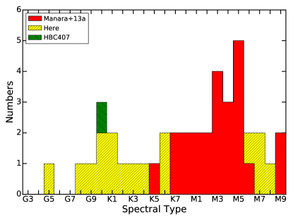
Figure 1: Histogram of the spectral type of the photospheric templates observed with X-Shooter and analyzed here, by MTR13, and by Manara et al. (2016).

3 Stellar properties

Table 1: Spectral types obtained from spectral indices

Object	Spectral type
	This work	Riddick	TiO	HH14
RXJ0445.8+1556	G5	…	…	…
RXJ1526.0-4501	G9	…	…	…
PZ99J160550.5-253313	K1	…	K5.7	K0.8
RXJ1508.6-4423	G8	…	…	…
PZ99J160843.4-260216	K0.5	…	K5.9	K0.5
RXJ1515.8-3331	K0.5	…	K5.6	K0.4
RXJ1547.7-4018	K3	…	K5.5	K2.7
RXJ0438.6+1546	K2	…	K5.6	K1.5
RXJ0457.5+2014	K1	…	K5.9	K1.2
RXJ1538.6-3916	K4	…	K5.7	K4.5
RXJ1540.7-3756	K6	…	K6.5	K9.5
RXJ1543.1-3920	K6	…	K6.4	K8.9
LM717	M6.5	M6.4	M6.4	M6.7
LM601	M7.5	M7.2	M7.7	M7.5
J11195652-7504529	M7	M6.9	M7.0	M7.3
CHSM17173	M8	M7.7	M7.3	M8.0

3.1 Spectral type classification using spectral indices

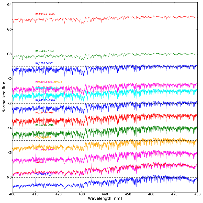
Figure 11: Spectra of Class III YSOs ordered according to their spectral type and normalized at 460 nm.

Spectral types were derived using spectral indices and these estimates have been further confirmed by visually inter-comparing the depth of temperature-sensitive molecular features in the spectra analyzed here. The spectral indices used are the same as in MTR13, which were selected among the indices provided by Riddick et al. (2007), and augmented with other spectral indices by Herczeg & Hillenbrand (2014, hereafter HH14) and the TiO index by Jeffries et al. (2007). These additional indices are particularly useful to assign a spectral type to stars of K- and early M- spectral type, which correspond to a range of stellar temperatures to which the Riddick et al. (2007) indices, developed for later-type objects, are not sensitive. The TiO index by Jeffries et al. (2007), in particular, is sensitive to spectral types K5, or later. The spectral type was thus assigned using the indices by HH14 for stars with spectral type between K0 and K5, the TiO index for stars with K6 and later K spectral type, and the mean values of the three sets of indices for the M spectral type objects. All values were rounded to half a subclass. The values derived with the different indices are reported in Table 1. The spectra of the objects are shown, ordered by spectral type, in Fig. 11-13.

Table 2: Stellar parameters derived for the targets analyzed in this work

Object	RA(2000)	DEC(2000)	$d$	SpT	Teff	log($L_{\star}/L_{\odot}$)	$d_{\rm TGAS}$	log($L_{\star}/L_{\odot}$)TGAS
	h   :m   :s	∘   ’   ”	[pc]		[K]		[pc]
RXJ0445.8+1556	04:45:51.29	+15:55:49.69	140	G5	5770	0.485	141$\pm$4	0.497
RXJ1526.0-4501	15:25:59.65	$-$45:01:15.72	150	G9	5410	$-$0.061	147$\pm$5	$-$0.073
PZ99J160550.5-253313	16:05:50.64	$-$25:33:13.60	145	K1	5000	$-$0.007	105$\pm$6	$-$0.287
RXJ1508.6-4423	15:08:37.75	$-$44:23:16.95	150	G8	5520	0.043	148$\pm$12	0.031
PZ99J160843.4-260216	16:08:43.41	$-$26:02:16.84	145	K0.5	5050	0.140	152$\pm$12	0.181
RXJ1515.8-3331	15:15:45.36	$-$33:31:59.78	150	K0.5	5050	0.098	…	…
RXJ1547.7-4018	15:47:41.76	$-$40:18:26.80	150	K3	4730	$-$0.081	135$\pm$4	$-$0.173
RXJ0438.6+1546	04:38:39.07	+15:46:13.61	140	K2	4900	$-$0.024	145$\pm$5	0.006
RXJ0457.5+2014	04:57:30.66	+20:14:29.42	140	K1	5000	$-$0.150	…	…
RXJ1538.6-3916	15:38:38.36	$-$39:16:54.08	150	K4	4590	$-$0.217	…	…
RXJ1540.7-3756	15:40:41.17	$-$37:56:18.54	150	K6	4205	$-$0.405	…	…
RXJ1543.1-3920	15:43:06.25	$-$39:20:19.5	150	K6	4205	$-$0.397	…	…
LM717	11:08:02.34	$-$76:40:34.3	160	M6.5	2935	$-$1.750	…	…
LM601	11:12:30.99	$-$76:53:34.2	160	M7.5	2795	$-$2.229	…	…
J11195652-7504529	11:19:56.52	$-$75:04:52.9	160	M7	2880	$-$2.177	…	…
CHSM17173	11:10:22.26	$-$76:25:13.8	160	M8	2710	$-$1.993	…	…

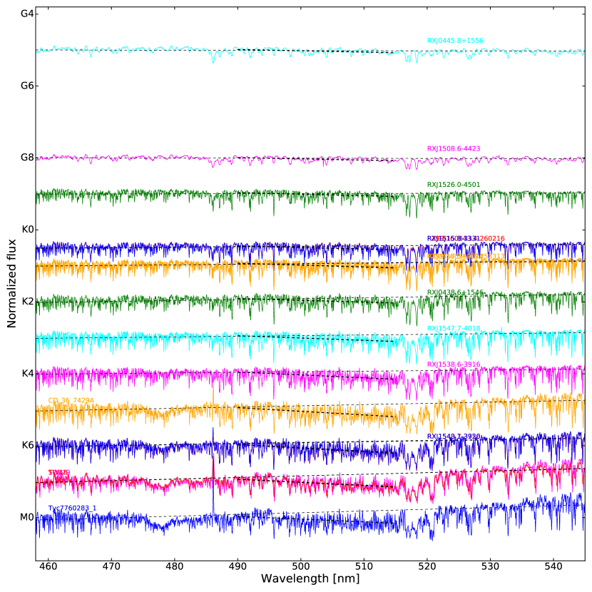
Figure 12: Spectra of Class III YSOs ordered according to their spectral type and normalized at 460 nm.

For the classification of the objects with G spectral type we used a method introduced by HH14. We join with a straight line the continuum emission at $\lambda\lambda$ 460 nm and 540 nm and between $\lambda\lambda$ 490 nm and 515 nm. We then compute the distance between these two lines at $\lambda$ = 515 nm. This distance increases with the spectral type for G and K stars, as shown in Fig. 12. This method allows us to classify G-type objects and, in turn, confirms the classification for K-type objects.

The final values of spectral type for the targets, and the corresponding effective temperatures, are reported in Table 2. The uncertainties on the spectral type are typically one sub-class for objects of G and K spectral types in our sample, and half a sub-class for M-type objects. Our estimates are typically consistent within one spectral sub-class with those from the literature (cf. Table 7), and different by two sub-classes at most. We show in Fig. 1 the histogram of the spectral types of the targets discussed here together with those analyzed by MTR13. When considered together, these libraries are now covering the whole range of spectral type from G8 to M9.5 with at least one template per spectral sub-class.

3.2 Extinction estimate

The targets analyzed here were selected to have negligible extinction ($A_{V}<$0.5 mag). We verify this assumption with two methods.

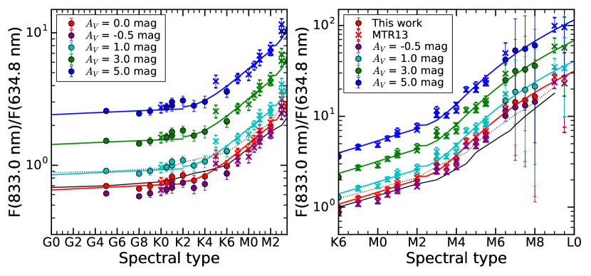
Figure 2: $F_{\rm red}=F(833.0{\rm nm})/F(634.8{\rm nm})$ ratio calculated for the ClassIII spectra analyzed here (circles) and by MTR13 (crosses). Different colors refer to values of $F_{\rm red}$ calculated on spectra reddened with increasing values of $A_{V}$, from 0 mag to 5 mag, as reported in the legend. The data reported as $A_{V}$ = -0.5 mag are obtained by de-reddening the spectrum by $A_{V}$ = 0.5 mag. The black solid line is the value of $F_{\rm red}$ derived by HH14 for $A_{V}$ = 0 mag, and the dotted line for $A_{V}$ = 1 mag. The colored lines are our new estimates of this ratio, which are reported in Table 10.

First, we compare the observed spectra to BT-Settl models (Allard et al., 2011) with the same temperature as the target and with log$g$=4.0 reddened using the extinction law by Cardelli et al. (1989) and $R_{V}$=3.1 with increasing values of $A_{V}$ in steps of 0.1 mag, and normalized at 750 nm to the continuum of the observed spectra. The value of $A_{V}$ at which the squared difference between the target and the model is minimized is then chosen. This method, when applied to G- and K-type objects, leads to values of $A_{V}$=0 mag for RXJ1508.6-4423, RXJ1547.7-4018, RXJ1538.6-3916, and RXJ1540.7-3756, of $A_{V}$=0.1 mag for RXJ1526.0-4501 and RXJ1543.1-3920, of $A_{V}$=0.2 mag for PZ99J160550.5-253313, PZ99J160843.4-260216, RXJ1515.8-3331, and RXJ0457.5+2014, of $A_{V}$=0.3 mag for RXJ0438.6+1546 and $A_{V}$=0.4 mag for RXJ0445.8+1556. These values have typically 1$\sigma$ uncertainties of 0.1 mag, and of 0.2 mag for the highest values. The values of extinction are thus, in all cases, smaller than 0.5 mag, and compatible with $A_{V}$=0 mag within, at most, 3$\sigma$. In the case of the four late-M-type objects, the agreement between the synthetic spectra and the observed one is not good. In particular, it is not possible to have a good agreement in both the near-infrared part of the spectra ($\lambda>1000$ nm) and the optical part ($\lambda>500$ nm) simultaneously. To check the values of $A_{V}$ we use a normalization at 1040 nm, which allows us to find a better match in the near-infrared part of the spectrum. We obtain $A_{V}$=1.3, 0.3, 0.9, and 0.6 mag for LM717, LM601, J11195652-7504529, and CHSM17173, respectively. However, these values are rather uncertain and are highly susceptible to the choice of the normalization wavelength, of the reddening law, and to the uncertainties in the models. We note that the values of $A_{V}$ estimated from the near-infrared colors for these late-type targets by Luhman (2007) are of 0 mag for all the objects apart from LM717, which was estimated at $A_{V}$=0.4 mag (see Table 7). Differences in the values of $A_{V}$ derived from near-infrared or optical spectra could be due to several physical properties of the objects, such as the presence of cold spots on the stellar surface (e.g., Stauffer et al., 2003; Vacca & Sandell, 2011; Pecaut, 2016; Gully-Santiago et al., 2017), which make the targets appear to be of later types in red spectra than in blue spectra.

An independent estimate of $A_{V}$ can be obtained from the ratio $F_{\rm red}=F(833.0{\rm nm})/F(634.8{\rm nm})$, as first suggested by HH14. This ratio is sensitive to $A_{V}$ and depends on the spectral type of the object. Fig. 2 shows the observed values for the objects analyzed here together with those in MTR13 , as well as the values obtained after applying a reddening correction with increasing values of $A_{V}$ from 0 mag to 5 mag, using the reddening law by Cardelli et al. (1989) and $R_{V}$=3.1. We also show the value of $F_{\rm red}$ after de-reddening the spectra by $A_{V}$ = 0.5 mag, reported on the plot as a negative value of $A_{V}$. On the same figure we show the values of this ratio calculated by HH14 for $A_{V}$ = 0 mag and 1 mag. The observed values of $F_{\rm red}$ are consistent with our assumption that $A_{V}\sim 0$ mag for spectral types earlier than M. As for the comparison with synthetic spectra, the values of $A_{V}$ for objects with G- and K spectral type are negligible. There are, however, differences in the M sub-class range. This could be due to the larger uncertainty in the estimate of this ratio in the analysis by HH14, who used both synthetic spectra and observed spectra of dwarfs to calibrate the index. Since synthetic spectra are not reliable in this spectral-type range (e.g., Da Rio et al., 2010; Bell et al., 2012), we argue that all the spectra of our targets are compatible with having negligible extinction, that is, $A_{V}<$ 0.5 mag, and we use our data to re-calibrate the values of $F_{\rm red}$ as a function of spectral type and $A_{V}$. The new values of $F_{\rm red}$ are reported in Table 10.

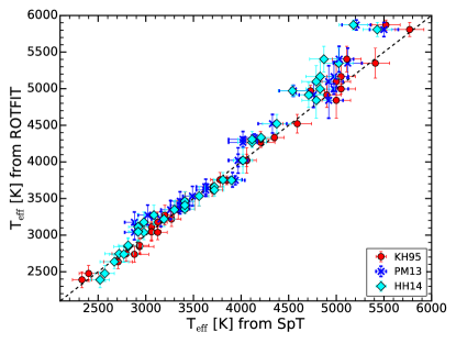
Figure 3: Comparison between temperatures from spectral types and from ROTFIT for the objects analyzed by MTR13, who reported the spectral type for these targets, and by Stelzer et al. (2013a) who presented the ROTFIT analysis, and for those analyzed here. The relations between spectral type and temperature are those used by Manara et al. (2013a), labeled as ‘KH95’ as it is mainly based on Kenyon & Hartmann (1995), as discussed in the text, the one by Pecaut & Mamajek (2013), labeled as ‘PM13’, and the one by Herczeg & Hillenbrand (2014), labeled as ‘HH14’. The relation by Pecaut & Mamajek (2013) is not available for spectral types later than M5.

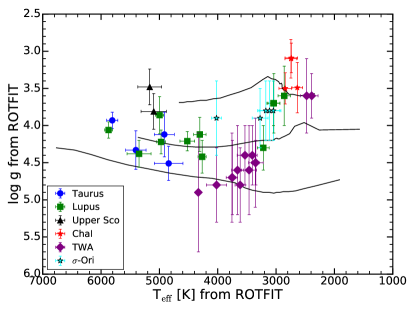
Figure 4: $\log g$–$T_{\rm eff}$  diagram for the targets analyzed here and by Stelzer et al. (2013a) showing the values derived with ROTFIT. Isochrones for 1, 10, and 100 Myr (from top to bottom) are from Baraffe et al. (2015).

3.3 Photospheric properties from ROTFIT

The X-Shooter spectra have sufficient spectral resolution and wavelength coverage to measure photospheric properties, namely the effective temperature ($T_{\rm eff}$), the surface gravity ($\log g$), the projected rotational velocity ($v\sin i$), and the radial velocity (RV) of the targets. We perform this analysis on the objects of our sample, including HBC407, using the ROTFIT tool (e.g., Frasca et al., 2015, 2017), which was also applied by Stelzer et al. (2013a) to analyze the Class III spectra of MTR13. This analysis tool is based on the search for the best template spectrum that reproduces the target spectrum by minimizing the $\chi^{2}$ of the difference between observed and template in specific spectral segments. We adopted as templates a grid of BT-Settl spectra (Allard et al., 2011) with solar iron abundance according to the Asplund et al. (2009) solar mixture and effective temperature in the range 2000–6000 K and $\log g$  from 5.5 to 0.5 dex. The tool is run setting the veiling to zero in all targets, since they are non-accreting objects. For the G- and K-type objects both the VIS and UVB arms have been used in the analysis with ROTFIT, while the VIS arm contains sufficient lines to analyze the colder objects in the sample. For the latter objects, only the VIS arm is used because of the lower S/N of the spectra in the UVB arm. The spectral intervals analyzed with ROTFIT contain features that are sensitive to the effective temperature and/or $\log g$, such as the Na i doublet at $\lambda\approx 8190$ Å and the K i doublet at $\lambda\approx 7660-7700$ Å. The code also allows us to measure the $v\sin i$  by $\chi^{2}$ minimization applied to spectral segments devoid of broad lines. The photospheric parameters derived with ROTFIT are reported in Table 3. For completeness, we include also the values of $v\sin i$  and RV, even if they are not used in the remainder of this paper.

Fig. 3 shows the comparison between $T_{\rm eff}$ derived with ROTFIT and the one obtained by converting the spectral type determined as in Sect. 3.1 using different relations between spectral type and $T_{\rm eff}$. We use here the relation by Kenyon & Hartmann (1995) for objects with spectral type in the G and K classes, and by Luhman et al. (2003) for later-type objects, in line with the analysis by MTR13 and Stelzer et al. (2013a), the one by Pecaut & Mamajek (2013) for 5-30 Myr-old objects, and the one by HH14 for young stars. The values obtained with these two methods using the combined relations of Kenyon & Hartmann (1995) and Luhman et al. (2003) agree within the 1$\sigma$ uncertainties for all targets except RXJ1508.6-4423, HBC407, and RXJ1547.7-4018. Other relations result in larger deviations especially for the stars with earliest types, which are, however, still within 3$\sigma$.

Fig. 4 shows the log$g$-$T_{\rm eff}$ plane for all targets in this work and those analyzed by Stelzer et al. (2013a), overplotted with theoretical isochrones by Baraffe et al. (2015). All the targets are compatible within the uncertainties of the parameters with being young objects with ages $\lesssim$ 10 Myr. These values of log$g$ derived here are thus compatible with the fact that these objects are PMS, and thus closer to luminosity class IV. We note that the coldest stars, thus with lower masses, have smaller values of log$g$, as noted also by Stelzer et al. (2013a). This would suggest a younger age for the objects, and we come back to this point in Sect. 3.4.

Table 3: Photospheric parameters derived with ROTFIT

Object	$T_{\rm eff}$	$\sigma(T_{\rm eff})$	log$g$	$\sigma$(log$g$)	vsin$i$	$\sigma$(vsin$i$)	RV	$\sigma$(RV)
	[K]	[K]	[cgs]	[cgs]	[km/s]	[km/s]	[km/s]	[km/s]
RXJ0445.8+1556	5808	96	3.93	0.11	117.1	7.8	17.6	7.4
RXJ1526.0-4501	5349	205	4.38	0.18	25.0	1.0	5.7	2.0
PZ99J160550.5-253313	5097	218	3.81	0.24	13.0	6.0	-1.5	1.7
RXJ1508.6-4423	5871	68	4.06	0.11	130,2	9.2	7.9	10.1
PZ99J160843.4-260216	5166	204	3.48	0.24	42.5	1.1	-4.3	2.5
RXJ1515.8-3331	4997	71	3.86	0.25	22.3	1.0	2.0	1.9
RXJ1547.7-4018	4971	75	4.22	0.16	11.1	1.0	2.9	1.7
RXJ0438.6+1546	4915	170	4.12	0.30	26.3	1.0	18.6	1.9
RXJ0457.5+2014	4841	244	4.51	0.23	35.6	1.2	13.4	2.1
RXJ1538.6-3916	4522	127	4.21	0.13	1.0	2.0	2.6	1.7
RXJ1540.7-3756	4267	70	4.42	0.22	19.1	1.0	1.7	1.9
RXJ1543.1-3920	4308	107	4.12	0.23	12.1	1.0	4.4	1.8
LM717	2843	107	3.50	0.21	19.0	21.0	23.2	2.5
J11195652-7504529	2738	109	3.09	0.20	44.0	19.0	15.1	5.6
HBC407	5404	175	4.33	0.26	10.0	1.0	19.1	1.7

3.4 Stellar luminosity

The stellar luminosities are obtained with the same procedure as in MTR13. The flux of the observed X-Shooter spectrum is integrated over the whole wavelength range, apart from the telluric bands in the NIR arm, where the continuum of the spectrum is interpolated with a straight line. The flux from the regions shortwards of $\sim$300 nm and at wavelengths longer than $\sim$2500 nm, which are not covered by X-Shooter, is obtained by integrating a BT-Settl synthetic spectrum Allard et al. (2011) with the same $T_{\rm eff}$ as the target and with log$g$ = 4.0, after matching it with the observed spectrum. We check that this method leads to results compatible with those obtained using the bolometric correction by HH14. The stellar luminosity ($L_{\star}$) is then derived from the bolometric flux using the distances to the star-forming regions where the targets are located, namely 140 pc for Taurus (HH14), 150 pc for Lupus (Comerón, 2008), 145 pc for Upper Sco (de Zeeuw et al., 1999), and 160 pc for Chamaeleon I (Luhman, 2008). The computed stellar luminosities are reported in Table 2. We also report in the last two columns of Table 2 the recent distance estimates from the TGAS catalog contained in the Data Release 1 (Gaia Collaboration et al., 2016) of the Gaia satellite (Gaia Collaboration et al., 2016), as well as the stellar luminosity corresponding to these revised distances. Distances obtained from parallax measurements are available for seven targets, with only the distance to PZ99J160550.5-253313 which significantly differs from the ones usually assumed for these objects. The revised distance to this object would change its age from $\sim$15 Myr to $\sim$30 Myr according to the evolutionary models by Siess et al. (2000).

The Hertzsprung-Russel diagram (HRD) is shown in Fig. 5, with the evolutionary tracks of Baraffe et al. (2015) superimposed. This diagram shows an apparent mass-dependent isochronal age trend, with lower-mass stars being typically $\sim$1-10 Myr old, and stars with $M_{\star}$$\gtrsim$0.8 $M_{\odot}$ being $\sim$10-30 Myr old. This trend is observed even in objects belonging to the same star-forming region, for example, Lupus, and is in line with other observations in different star-forming regions (e.g., Bell et al., 2014; Herczeg & Hillenbrand, 2015; Pecaut & Mamajek, 2016), and with the log$g$-$T_{\rm eff}$ trend we see in Fig. 4. Possible origins for this dependence are the presence of spots on the stellar surface, or the effects of convection related to the presence of magnetic fields, or the effects of accretion during the pre-main sequence evolutionary phase, which are currently being implemented in evolutionary models (e.g., Somers & Pinsonneault, 2015; Feiden, 2016; Baraffe et al., 2017). It is also worth noting that the ages inferred from the log$g$-$T_{\rm eff}$ relation differ from those inferred from the HRD. For example, the targets in the Chamaeleon I region are always younger than 1 Myr in the former, and have age $\sim$1-10 Myr in the latter diagram. This discrepancy is in line with previous results (e.g., Slesnick et al., 2006).

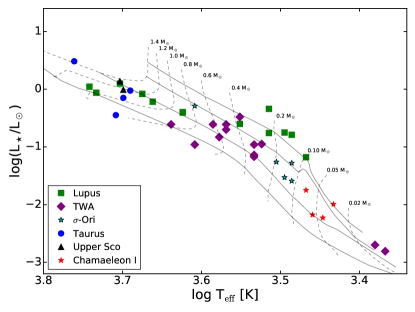
Figure 5: HR diagram of the objects analyzed here and those by MTR13, where $T_{\rm eff}$ is obtained from the spectral type. The models by Baraffe et al. (2015) are also shown. The isochrones are the 1.2, 3, 10, and 30 Myr ones.

Table 4: Photospheric colors of young non-accreting stars

Spectral	$U-B$		$B-V$		$V-R$		$R-I$		$V-J$		$J-H$		$H-Ks$
Type	[mag]	[mag]	[mag]	[mag]	[mag]	[mag]	[mag]	[mag]	[mag]	[mag]	[mag]	[mag]	[mag]	[mag]
G5	0.30	${}^{+0.94}_{-0.45}$	0.72	${}^{+0.24}_{-0.22}$	0.44	${}^{+0.35}_{-0.19}$	0.43	${}^{+0.15}_{-0.12}$	1.46	${}^{+1.18}_{-0.50}$	0.42	${}^{+0.17}_{-0.21}$	0.00	${}^{+0.15}_{-0.18}$
G6	0.25	${}^{+0.71}_{-0.32}$	0.71	${}^{+0.22}_{-0.15}$	0.42	${}^{+0.29}_{-0.15}$	0.41	${}^{+0.13}_{-0.10}$	1.40	${}^{+0.83}_{-0.38}$	0.41	${}^{+0.16}_{-0.14}$	0.04	${}^{+0.11}_{-0.16}$
G7	0.25	${}^{+0.55}_{-0.24}$	0.73	${}^{+0.18}_{-0.11}$	0.42	${}^{+0.23}_{-0.12}$	0.41	${}^{+0.11}_{-0.07}$	1.40	${}^{+0.71}_{-0.30}$	0.42	${}^{+0.14}_{-0.10}$	0.06	${}^{+0.09}_{-0.14}$
G8	0.29	${}^{+0.46}_{-0.19}$	0.77	${}^{+0.14}_{-0.10}$	0.44	${}^{+0.17}_{-0.10}$	0.42	${}^{+0.08}_{-0.06}$	1.44	${}^{+0.58}_{-0.29}$	0.44	${}^{+0.12}_{-0.09}$	0.08	${}^{+0.08}_{-0.12}$
G9	0.35	${}^{+0.35}_{-0.19}$	0.82	${}^{+0.12}_{-0.09}$	0.46	${}^{+0.13}_{-0.08}$	0.44	${}^{+0.07}_{-0.05}$	1.51	${}^{+0.46}_{-0.25}$	0.47	${}^{+0.10}_{-0.08}$	0.08	${}^{+0.08}_{-0.10}$
K0	0.44	${}^{+0.29}_{-0.17}$	0.87	${}^{+0.09}_{-0.08}$	0.49	${}^{+0.10}_{-0.08}$	0.46	${}^{+0.06}_{-0.05}$	1.60	${}^{+0.41}_{-0.23}$	0.50	${}^{+0.09}_{-0.07}$	0.09	${}^{+0.08}_{-0.08}$
K1	0.54	${}^{+0.26}_{-0.16}$	0.93	${}^{+0.09}_{-0.09}$	0.52	${}^{+0.10}_{-0.08}$	0.49	${}^{+0.05}_{-0.06}$	1.72	${}^{+0.38}_{-0.25}$	0.53	${}^{+0.08}_{-0.07}$	0.10	${}^{+0.08}_{-0.07}$
K2	0.65	${}^{+0.27}_{-0.16}$	0.99	${}^{+0.10}_{-0.09}$	0.56	${}^{+0.10}_{-0.09}$	0.52	${}^{+0.05}_{-0.06}$	1.86	${}^{+0.37}_{-0.24}$	0.56	${}^{+0.08}_{-0.08}$	0.12	${}^{+0.08}_{-0.07}$
K3	0.76	${}^{+0.28}_{-0.18}$	1.06	${}^{+0.11}_{-0.08}$	0.60	${}^{+0.10}_{-0.09}$	0.56	${}^{+0.05}_{-0.06}$	2.01	${}^{+0.34}_{-0.24}$	0.60	${}^{+0.07}_{-0.08}$	0.14	${}^{+0.07}_{-0.07}$
K4	0.87	${}^{+0.25}_{-0.19}$	1.13	${}^{+0.11}_{-0.08}$	0.65	${}^{+0.10}_{-0.09}$	0.61	${}^{+0.06}_{-0.05}$	2.18	${}^{+0.35}_{-0.27}$	0.63	${}^{+0.07}_{-0.08}$	0.17	${}^{+0.07}_{-0.08}$
K5	0.95	${}^{+0.26}_{-0.20}$	1.20	${}^{+0.10}_{-0.08}$	0.70	${}^{+0.09}_{-0.10}$	0.67	${}^{+0.06}_{-0.05}$	2.36	${}^{+0.34}_{-0.27}$	0.65	${}^{+0.07}_{-0.08}$	0.20	${}^{+0.06}_{-0.08}$
K6	1.01	${}^{+0.28}_{-0.20}$	1.26	${}^{+0.08}_{-0.09}$	0.75	${}^{+0.09}_{-0.09}$	0.75	${}^{+0.06}_{-0.05}$	2.57	${}^{+0.33}_{-0.25}$	0.67	${}^{+0.07}_{-0.07}$	0.22	${}^{+0.06}_{-0.07}$
K7	1.04	${}^{+0.25}_{-0.20}$	1.33	${}^{+0.07}_{-0.09}$	0.80	${}^{+0.08}_{-0.09}$	0.85	${}^{+0.07}_{-0.04}$	2.80	${}^{+0.33}_{-0.23}$	0.68	${}^{+0.07}_{-0.06}$	0.24	${}^{+0.05}_{-0.07}$
M0	1.03	${}^{+0.25}_{-0.18}$	1.38	${}^{+0.06}_{-0.09}$	0.86	${}^{+0.08}_{-0.08}$	0.96	${}^{+0.06}_{-0.04}$	3.07	${}^{+0.34}_{-0.21}$	0.69	${}^{+0.06}_{-0.06}$	0.25	${}^{+0.05}_{-0.07}$
M1	1.01	${}^{+0.25}_{-0.14}$	1.42	${}^{+0.07}_{-0.08}$	0.92	${}^{+0.08}_{-0.07}$	1.10	${}^{+0.06}_{-0.03}$	3.38	${}^{+0.33}_{-0.18}$	0.70	${}^{+0.05}_{-0.06}$	0.26	${}^{+0.05}_{-0.06}$
M2	0.99	${}^{+0.25}_{-0.12}$	1.46	${}^{+0.08}_{-0.07}$	1.01	${}^{+0.08}_{-0.06}$	1.26	${}^{+0.06}_{-0.03}$	3.75	${}^{+0.30}_{-0.16}$	0.69	${}^{+0.05}_{-0.06}$	0.27	${}^{+0.05}_{-0.06}$
M3	0.99	${}^{+0.23}_{-0.10}$	1.51	${}^{+0.08}_{-0.05}$	1.12	${}^{+0.09}_{-0.05}$	1.44	${}^{+0.06}_{-0.03}$	4.20	${}^{+0.30}_{-0.15}$	0.68	${}^{+0.05}_{-0.07}$	0.29	${}^{+0.05}_{-0.06}$
M4	1.01	${}^{+0.21}_{-0.12}$	1.58	${}^{+0.08}_{-0.05}$	1.28	${}^{+0.09}_{-0.05}$	1.63	${}^{+0.04}_{-0.04}$	4.75	${}^{+0.30}_{-0.13}$	0.66	${}^{+0.05}_{-0.06}$	0.30	${}^{+0.05}_{-0.06}$
M5	1.05	${}^{+0.19}_{-0.16}$	1.68	${}^{+0.07}_{-0.06}$	1.48	${}^{+0.09}_{-0.05}$	1.83	${}^{+0.03}_{-0.05}$	5.40	${}^{+0.28}_{-0.16}$	0.64	${}^{+0.06}_{-0.05}$	0.32	${}^{+0.05}_{-0.05}$
M6	1.06	${}^{+0.18}_{-0.21}$	1.79	${}^{+0.06}_{-0.08}$	1.73	${}^{+0.08}_{-0.07}$	2.02	${}^{+0.02}_{-0.06}$	6.13	${}^{+0.21}_{-0.20}$	0.62	${}^{+0.07}_{-0.04}$	0.34	${}^{+0.06}_{-0.05}$
M7	1.04	${}^{+0.20}_{-0.25}$	1.90	${}^{+0.05}_{-0.10}$	2.01	${}^{+0.08}_{-0.08}$	2.20	${}^{+0.03}_{-0.07}$	6.92	${}^{+0.23}_{-0.25}$	0.61	${}^{+0.08}_{-0.05}$	0.37	${}^{+0.07}_{-0.05}$
M8	0.93	${}^{+0.40}_{-0.31}$	1.98	${}^{+0.07}_{-0.12}$	2.31	${}^{+0.10}_{-0.11}$	2.36	${}^{+0.05}_{-0.08}$	7.72	${}^{+0.32}_{-0.29}$	0.63	${}^{+0.09}_{-0.07}$	0.42	${}^{+0.08}_{-0.06}$
M9	0.69	${}^{+0.81}_{-0.37}$	2.02	${}^{+0.16}_{-0.14}$	2.62	${}^{+0.19}_{-0.13}$	2.47	${}^{+0.10}_{-0.09}$	8.48	${}^{+0.65}_{-0.32}$	0.67	${}^{+0.12}_{-0.13}$	0.50	${}^{+0.10}_{-0.12}$

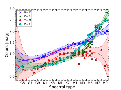
Figure 6: Colors as a function of spectral type for the objects discussed here. The best fit for each color and the 3$\sigma$ confidence intervals are shown with a solid line and a shaded region. The solid purple line is the $B-V$ color for 5-30 Myr-old pre-main sequence stars by Pecaut & Mamajek (2013).

4 Photospheric colors of young stars

The absolutely flux-calibrated X-shooter spectra of our targets, with their large, simultaneous wavelength coverage and high signal-to-noise are perfectly suited to compute broad-band colors for young stars and to be used to study variations of the extinction or the presence of spots on the surface of young objects (e.g., Gully-Santiago et al., 2017). This kind of study relies on the knowledge of the intrinsic colors of the star, which are gravity dependent (e.g., Luhman et al., 2003). These spectra of non-accreting stars are thus ideal for calibrating the relation between spectral type and photospheric color for sub-giants.

We perform synthetic photometry on the spectra in the following bands: Johnson $U$, $B$, and $V$, Cousins $R$ and $I$, and 2MASS $J$, $H$, $Ks$, using the throughputs provided with the TA-DA tool (Da Rio & Robberto, 2012). We then plot the optical colors $B-V$, $V-R$, $U-B$, and $R-I$ for our targets as a function of their spectral type in Fig. 6, and similarly for the near-infrared $J-H$ and $H-K$ colors in Fig. 7. We show the $B-V$ color for pre-main sequence stars derived by Pecaut & Mamajek (2013), and the infrared colors by Pecaut & Mamajek (2013) and Luhman et al. (2003) in the plots. These photospheric colors are consistent within uncertainties with our estimate. We check that a value of $A_{V}$ larger than 0 mag, and up to 0.5 mag, would result in differences in the colors of up to 0.1 mag for the $U-B$ and $B-V$ colors, and less for the other colors. These differences are well within the uncertainties in the relation between spectral type and color we derive. In general the colors increase for later spectral types, but the dependence on the spectral type is usually not a simple relation. For this reason, and in order not to generate bias due to prior assumption on the dependence of a color on the spectral type, we decided to use a non-parametric method to fit the data. In particular, we adopt a local second degree polynomial regression with a Gaussian kernel, using the Python module pyqt_fit.npr_methods.LocalPolynomialKernel. We then bootstrap the result of this fit and derive the 3$\sigma$ confidence level for the fit, which is shown as a shaded region around the best fit on the plots. The most uncertain color is the $U-B$ color, with typical 3-$\sigma$ uncertainties of $\pm$0.3 mag. The largest uncertainty in the colors for later spectral types is due to the low S/N of the spectra, while for those at earlier spectral types the uncertainty is due to the low number of objects.

The relations between photospheric colors and spectral type for young stars, that is, sub-giants, calibrated on our spectra are reported in Table 4. These are given as a function of spectral type since they are independent on the relation between spectral type and effective temperature.

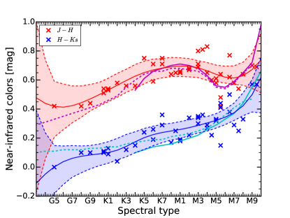
Figure 7: Colors as a function of spectral type for the objects discussed here. The best fit for each color and the 3$\sigma$ confidence intervals are shown with a solid line and a shaded region. The solid purple and cyan lines are the $J-H$ and $H-K$ photospheric colors for pre-main sequence stars by Luhman et al. (2003), while the dashed lines are the same colors for 5-30 Myr-old pre-main sequence stars by Pecaut & Mamajek (2013).

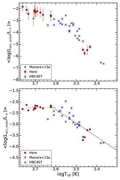
Figure 8: Luminosity of chromospheric emission lines converted into $L_{\rm acc,noise}$ as a function of the logarithm of the effective temperature obtained from the spectral type for all the ClassIII targets discussed here. In the bottom plot the values of $L_{\rm acc,noise}$ are normalized by the stellar luminosity, and the lines represent the fit reported in Equation 1.

5 Impact of chromospheric emission lines on accretion rate estimates

Young non-accreting stars typically show the well-known emission lines that characterize cromospheric activity; namely the hydrogen Balmer lines, most prominently the H$\alpha$ and H$\beta$ lines, the calcium lines, in particular the Ca II infrared triplet (CaIRT) lines at $\lambda\lambda\sim$ 849.80 - 854.21 - 866.21 nm, the Ca K line at $\lambda\sim$ 393.37 nm and the Ca H line at $\lambda\sim$ 396.85 nm, and the helium lines, in particular the one at $\lambda\sim$ 587.6 nm. No emission lines due to chromospheric activity are typically present at infrared wavelengths. The chromospheric calcium lines usually appear as a narrow emission component inside a broad and pronounced photospheric absorption line, and similarly the hydrogen Balmer lines for objects hotter than $\sim$4000 K.

The objects analyzed here span a large range of temperatures, and the presence of the aforementioned lines strongly depends on this parameter. The later-type objects with M spectral type in our sample show the H$\alpha$ and H$\beta$ lines in emission, with the only exception of LM601 where the H$\beta$ line is not detected possibly due to the low S/N of this spectrum at the wavelength of H$\beta$. None of these targets instead present emission in the calcium lines, not even when taking into account the photospheric absorption. The very low signal to noise ratio at the wavelengths of the H and K lines prevents detection of these lines for these cold targets, while the CaIRT lines are not detected even if the S/N is larger than 20 at the wavelengths of these transitions. We measure the flux of the H$\alpha$ and H$\beta$ lines in these targets by directly integrating the continuum-subtracted spectra, which leads to values consistent with those obtained by integrating the emission profiles in the spectrum obtained by the subtraction of the non-active template, since the underlying photospheric absorption is negligible in these cases.

On the other hand, the hotter objects with G and K spectral type in our sample always show prominent calcium and H$\alpha$ emission lines in reversal on the photospheric absorption lines. Thus, the subtraction of the photospheric template, taken as the best-fitting BT-Settl spectrum determined by ROTFIT, is mandatory to measure the flux of these lines. In three objects, namely RXJ1508.6-4423, RXJ1540.7-3756, and RXJ1543.1-3920, the H$\beta$ line is also detected after subtracting the photospheric absorption line, and we can measure their fluxes. In the following, we consider the flux from all the detected lines in the analysis, with the only exception being the Ca H line, as this is usually blended with that of H$\epsilon$ . Although the latter is expected to be faint, the decomposition of the profile is complicated given the projected rotational velocity of our targets and the resolution of our spectra, and we thus prefer to neglect this line in the analysis. The measured flux for these lines is reported in Table 6.

Following MTR13, we apply the relations between line luminosity and accretion luminosity from Alcalá et al. (2014) to the luminosity of the lines produced in the chromospheres. As showed by Rigliaco et al. (2012) and Alcalá et al. (2014), the mean value of the accretion luminosity derived with these relations using multiple emission lines is consistent with the accretion luminosity obtained with the more direct method of directly measuring the excess emission in the Balmer continuum region. We thus want to obtain the equivalent accretion luminosity a typical chromosphere of a non-accreting young star would lead to by taking the mean value of as many emission lines as are present in the spectra. We call this equivalent accretion luminosity a “noise” on the accretion luminosity ($L_{\rm acc,noise}$). We note that, after this conversion, the values of $L_{\rm acc,noise}$ obtained using the H$\alpha$ line luminosity are systematically lower by $\sim$0.5 dex than those derived with the calcium lines, and $\sim$ 0.3 dex lower than those obtained using the H$\beta$ line. The discrepancy between the hydrogen Balmer and the calcium lines has already been reported by MTR13. The values of $L_{\rm acc,noise}$ derived from the four calcium lines analyzed here are instead generally consistent with one another within $\sim$0.2 dex. The two exceptions to these general properties are RXJ1508.6-4423 and RXJ0445.8+1556. The former is one of the three hotter objects in our sample where the H$\beta$ line is detected. We see that the values of $L_{\rm acc,noise}$ derived from the different lines for this object all agree with one another within $\sim$0.2 dex, while the values obtained using the Ca K line are higher than the mean value of $L_{\rm acc,noise}$ by $\sim$0.7 dex. Similarly, the values of $L_{\rm acc,noise}$ obtained for RXJ0445.8+1556 using the H$\alpha$ and CaIRT lines are discrepant by less than $\sim$0.3 dex, while the Ca K line flux leads to a value of $L_{\rm acc,noise}$ higher by $\sim$ 0.7 dex. Since we are interested here in the typical impact of the typical values of the chromospheric emission on the measurements of accretion, and that in accreting objects this is better constrained when multiple lines are used, we decided to include all the detected lines in the analysis, and to use the mean value of $L_{\rm acc,noise}$ of all these lines, which is reported in Table 6.

The dependence of $L_{\rm acc,noise}$ on T_eff, as well as the dependence of the stellar luminosity normalized $L_{\rm acc,noise}$ on $T_{\rm eff}$ is shown in Fig. 8. The four newly added targets with late M spectral type follow the same linear trend in the log($L_{\rm acc,noise}$/$L_{\star}$) versus log(T_eff) relation as found by MTR13. The relation flattens at temperatures larger than $\sim$4000 K, and can be expressed as:

$$\log(L_{\rm acc,noise}/L_{\star})=-2.3\pm 0.1\leavevmode\nobreak\ \leavevmode\nobreak\ \leavevmode\nobreak\ \leavevmode\nobreak\ \leavevmode\nobreak\ {\rm for\leavevmode\nobreak\ \leavevmode\nobreak\ \leavevmode\nobreak\ 4000<T_{eff}<5800K}\\ \log(L_{\rm acc,noise}/L_{\star})=(6.2\pm 0.5)\cdot\log T_{\rm eff}-(24.5\pm 1.9)\\ \leavevmode\nobreak\ \leavevmode\nobreak\ \leavevmode\nobreak\ \leavevmode\nobreak\ \leavevmode\nobreak\ {\rm for\leavevmode\nobreak\ \leavevmode\nobreak\ \leavevmode\nobreak\ T_{eff}\leq 4000K},$$ (1)

where the relation for low temperature is the one reported by MTR13. The values of $\log(L_{\rm acc,noise}/L_{\star})$ have a small dependence on the assumed distance of the targets due to the fact that $L_{\rm acc,noise}$ is not directly proportional to $L_{\rm line}$. However, the value of $L_{\rm acc,noise}$ reported for the objects with $T_{\rm eff}>$ 4000 K does not change even assuming the new distances from the Gaia TGAS catalog.

Since the relation between spectral type and $T_{\rm eff}$ for young stars is still debated in the literature (see Sect. 3.3), it is useful to provide also a relation between log($L_{\rm acc,noise}$/$L_{\star}$) and the spectral type, which is shown in Fig. 9. We perform the same analysis as for the dependence with $T_{\rm eff}$, and obtain the typical values of log($L_{\rm acc,noise}$/$L_{\star}$) as a function of the spectral type of the targets, which are reported in Table 5.

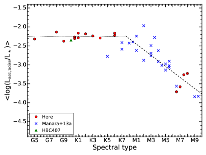
Figure 9: Luminosity of chromospheric emission lines converted into $L_{\rm acc,noise}$ and normalized by the stellar luminosity as a function of the spectral type for all the targets discussed here.

Table 5: Typical noise on the measurements of accretion induced by chromospheric emission

Spectral type	log($L_{\rm acc,noise}$/$L_{\star}$)
G5	-2.25 $\pm$ 0.07
G6	-2.25 $\pm$ 0.07
G7	-2.25 $\pm$ 0.07
G8	-2.25 $\pm$ 0.07
G9	-2.25 $\pm$ 0.07
K0	-2.25 $\pm$ 0.07
K1	-2.25 $\pm$ 0.07
K2	-2.25 $\pm$ 0.07
K3	-2.25 $\pm$ 0.07
K4	-2.25 $\pm$ 0.07
K5	-2.25 $\pm$ 0.07
K6	-2.25 $\pm$ 0.07
K7	-2.25 $\pm$ 0.07
M0	-2.31 $\pm$ 0.07
M1	-2.45 $\pm$ 0.08
M2	-2.60 $\pm$ 0.09
M3	-2.75 $\pm$ 0.11
M4	-2.89 $\pm$ 0.12
M5	-3.04 $\pm$ 0.13
M6	-3.19 $\pm$ 0.15
M7	-3.33 $\pm$ 0.16
M8	-3.48 $\pm$ 0.17
M9	-3.62 $\pm$ 0.19

The flattening of the relation for objects of spectral type earlier than about K7 was already noticed by MTR13, whose sample, however, included only a couple of stars earlier than K7. This is possibly related to the saturation of the chromospheric activity in hotter stars (see e.g., Stelzer et al., 2013a; Frasca et al., 2015). However, we want to stress that $L_{\rm acc,noise}$, computed following the same procedure used to measure $L_{\rm acc}$ in accreting stars, that is, averaging the values of $L_{\rm acc}$ derived from each detected emission line, is not an appropriate diagnostic of chromospheric activity, but is only a way to estimate the effect of chromospheric emission on the measurements of accretion rates. The analysis of the chromospheric properties of these objects is not among the aims of this work.

5.1 Implications for accretion rate estimates

The chromospheric emission of young stars derived here impacts the measurements of $L_{\rm acc}$ in accreting young stars and, in turn, of $\dot{M}_{\rm acc}$. It is particularly instructive to find the values of $\dot{M}_{\rm acc}$ at a given $M_{\star}$ corresponding to the typical chromospheric emission. We thus use the value of $L_{\rm acc,noise}$ for objects with $M_{\star}$$>$ 1 $M_{\odot}$ from Eq. 1 and convert this into $\dot{M}_{\rm acc}$ adopting the stellar luminosity, mass, and radius from one isochrone of the evolutionary models by Siess et al. (2000), similarly as done by MTR13 for lower-mass stars. This model is chosen as it extends to higher stellar masses than the more recent models by Baraffe et al. (2015), and it is thus more appropriate for this analysis. The resulting values of $\dot{M}_{\rm acc}$, which are the limit of the detectable accretion rate in chromospherically active young stars, are shown in Fig. 10 for the 3 Myr and 10 Myr isochrones by Siess et al. (2000), and together with the same limits derived by MTR13 for $M_{\star}$$<$1 $M_{\odot}$. In this plot we also show the measurements of $\dot{M}_{\rm acc}$ for the close to complete samples of Class II stars (i.e., with evidence of disks) in the Lupus (Alcalá et al., 2014, 2017) and Chamaeleon I (Manara et al., 2016, 2017) star-forming regions. The majority of targets show measured accretion rates well above the chromospheric limits. However, both samples include some Class II objects whose measured accretion rate is compatible or smaller than the expected chromospheric emission, and these are shown with empty symbols. The measured emission for these targets is thus probably dominated by chromospheric activity, and it is not possible to determine whether they are accreting or not. For this reason these targets have been defined as “dubious accretors” by Alcalá et al. (2017) and Manara et al. (2017).

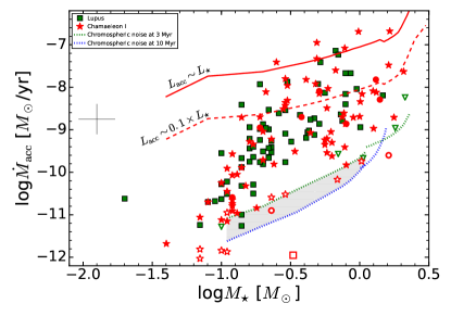
Figure 10: Compilation of mass accretion rates vs. stellar masses measured from VLT/X-Shooter spectra by Alcalá et al. (2014, 2017, green squares, Lupus sample) and by Manara et al. (2016, 2017, red stars, Chamaeleon I sample). The red solid and dashed lines show the values of mass accretion rates corresponding to objects whose accretion luminosity is respectively equal to the stellar luminosity or to 10% of it. The limits derived here due to chromospheric emission are shown with green and blue dotted lines for $\sim$3 Myr and $\sim$10 Myr old objects, respectively.

Table 6: Flux of emission lines and chromospheric noise

Object	$F_{\rm H\alpha}$	$F_{\rm H\beta}$	$F_{\rm CaK393.4nm}$	$F_{\rm Ca849.8nm}$	$F_{\rm Ca854.2nm}$	$F_{\rm Ca866.2nm}$	$\log L_{\rm acc,noise}$
RXJ0445.8+1556	(9.0$\pm$1.3)$\cdot 10^{-13}$	…	(6.9$\pm$1.3)$\cdot 10^{-13}$	(7.6$\pm$1.7)$\cdot 10^{-14}$	(6.6$\pm$1.4)$\cdot 10^{-14}$	(8.7$\pm$1.7)$\cdot 10^{-14}$	-1.8$\pm$0.3
RXJ1526.0-4501	(8.5$\pm$1.7)$\cdot 10^{-14}$	…	(9.1$\pm$3.1)$\cdot 10^{-14}$	(2.1$\pm$0.3)$\cdot 10^{-14}$	(3.2$\pm$0.4)$\cdot 10^{-14}$	(2.7$\pm$0.3)$\cdot 10^{-14}$	-2.4$\pm$0.4
PZ99J160550.5-253313	(1.3$\pm$0.2)$\cdot 10^{-13}$	…	(8.6$\pm$3.6)$\cdot 10^{-14}$	(4.2$\pm$0.5)$\cdot 10^{-14}$	(5.4$\pm$0.6)$\cdot 10^{-14}$	(4.4$\pm$0.5)$\cdot 10^{-14}$	-2.3$\pm$0.4
RXJ1508.6-4423	(6.6$\pm$0.7)$\cdot 10^{-13}$	(1.6$\pm$0.3)$\cdot 10^{-13}$	(3.2$\pm$0.6)$\cdot 10^{-13}$	(2.8$\pm$0.6)$\cdot 10^{-14}$	(3.1$\pm$0.5)$\cdot 10^{-14}$	(3.3$\pm$0.6)$\cdot 10^{-14}$	-2.1$\pm$0.3
PZ99J160843.4-260216	(2.0$\pm$0.3)$\cdot 10^{-13}$	…	(1.6$\pm$0.4)$\cdot 10^{-13}$	(5.0$\pm$0.6)$\cdot 10^{-14}$	(7.1$\pm$0.8)$\cdot 10^{-14}$	(6.2$\pm$0.7)$\cdot 10^{-14}$	-2.2$\pm$0.4
RXJ1515.8-3331	(1.2$\pm$0.2)$\cdot 10^{-13}$	…	(1.3$\pm$0.4)$\cdot 10^{-13}$	(4.2$\pm$0.5)$\cdot 10^{-14}$	(6.1$\pm$0.7)$\cdot 10^{-14}$	(5.4$\pm$0.6)$\cdot 10^{-14}$	-2.2$\pm$0.4
RXJ1547.7-4018	(1.1$\pm$0.2)$\cdot 10^{-13}$	…	(8.9$\pm$3.3)$\cdot 10^{-14}$	(3.1$\pm$0.4)$\cdot 10^{-14}$	(4.5$\pm$0.5)$\cdot 10^{-14}$	(3.9$\pm$0.4)$\cdot 10^{-14}$	-2.3$\pm$0.4
RXJ0438.6+1546	(1.7$\pm$0.2)$\cdot 10^{-13}$	…	(1.0$\pm$0.2)$\cdot 10^{-13}$	(5.4$\pm$0.6)$\cdot 10^{-14}$	(7.3$\pm$0.8)$\cdot 10^{-14}$	(6.0$\pm$0.6)$\cdot 10^{-14}$	-2.2$\pm$0.4
RXJ0457.5+2014	(1.5$\pm$0.2)$\cdot 10^{-13}$	…	(9.4$\pm$2.5)$\cdot 10^{-14}$	(3.7$\pm$0.5)$\cdot 10^{-14}$	(5.2$\pm$0.6)$\cdot 10^{-14}$	(4.4$\pm$0.6)$\cdot 10^{-14}$	-2.3$\pm$0.4
RXJ1538.6-3916	(5.2$\pm$0.9)$\cdot 10^{-14}$	…	(5.5$\pm$1.0)$\cdot 10^{-14}$	(2.3$\pm$0.3)$\cdot 10^{-14}$	(3.2$\pm$0.4)$\cdot 10^{-14}$	(3.0$\pm$0.3)$\cdot 10^{-14}$	-2.5$\pm$0.5
RXJ1540.7-3756	(6.4$\pm$0.9)$\cdot 10^{-14}$	(2.3$\pm$1.0)$\cdot 10^{-14}$	(3.7$\pm$0.5)$\cdot 10^{-14}$	(2.2$\pm$0.2)$\cdot 10^{-14}$	(3.0$\pm$0.3)$\cdot 10^{-14}$	(2.4$\pm$0.3)$\cdot 10^{-14}$	-2.6$\pm$0.4
RXJ1543.1-3920	(7.5$\pm$1.0)$\cdot 10^{-14}$	(3.5$\pm$1.8)$\cdot 10^{-14}$	(4.0$\pm$0.4)$\cdot 10^{-14}$	(2.3$\pm$0.2)$\cdot 10^{-14}$	(3.1$\pm$0.3)$\cdot 10^{-14}$	(2.7$\pm$0.3)$\cdot 10^{-14}$	-2.6$\pm$0.4
LM717	(9.9$\pm$0.5)$\cdot 10^{-16}$	(9.7$\pm$1.0)$\cdot 10^{-17}$	…	…	…	…	-5.5$\pm$0.1
LM601	(3.4$\pm$0.3)$\cdot 10^{-16}$	$<$1.352$\cdot 10^{-16}$	…	…	…	…	-5.5$\pm$0.4
J11195652-7504529	(5.8$\pm$0.4)$\cdot 10^{-16}$	(4.8$\pm$1.6)$\cdot 10^{-17}$	…	…	…	…	-5.8$\pm$0.2
CHSM17173	(1.59$\pm$0.06)$\cdot 10^{-15}$	(1.6$\pm$0.2)$\cdot 10^{-16}$	…	…	…	…	-5.2$\pm$0.1
HBC407	(3.1$\pm$0.7)$\cdot 10^{-14}$	…	…	(1.1$\pm$0.1)$\cdot 10^{-14}$	(1.6$\pm$0.2)$\cdot 10^{-14}$	(1.5$\pm$0.2)$\cdot 10^{-14}$	-2.8$\pm$0.6

6 Summary and conclusions

We present the analysis of new VLT/X-Shooter spectra of photospheric templates of young stars that complements the previous analysis by Manara et al. (2013a) by including objects with spectral types not covered in the previous work. All the spectra are available in reduced form on the CDS website, and they represent a complete set of photospheric templates of young stars with spectral type from G5 to M9.5 and with typically two or more spectra per spectral subclass. The spectra have all been analyzed homogeneously, with spectral types obtained by means of spectral indices and by comparing the relative strength of photospheric absorption features, as well as with an analysis with the ROTFIT tool to derive the photospheric properties ($T_{\rm eff}$, log$g$, $v$sin$i$, RV). We have shown that the two methods produce results in agreement with each other, and that the photospheric properties are compatible with the young ages of these objects. We see the presence of an apparent mass-related isochronal age dependence (younger age for lower-mass stars) when comparing the positions of our targets on the HRD with evolutionary models, as already noted in the literature.

Thanks to the broad wavelength coverage of our spectra and to their absolute flux calibration, we have derived photospheric colors in multiple bands ($U,B,V,R,I,J,H,K_{s}$) as a function of the spectral type. These colors are the first multi-band set of colors computed for a set of pre-main sequence stars, that is, sub-giants, with an ample coverage of spectral types and can be used as standard colors for this kind of object.

We have measured the flux of several emission lines due to chromospheric activity by properly subtracting the photospheric absorption lines. We have converted the flux of these lines into $L_{\rm acc,noise}$, which is the equivalent value of accretion luminosity one would obtain if this emission were due to accretion processes in young stars with disks. This value, which represents the typical lower limit on the measurable accretion rates in young stars, is independent to the stellar temperature for $T_{\rm eff}>4000$ K when normalized for the stellar luminosity. This is possibly related to the saturation of chromospheric emission in these young objects. On the other hand, our data confirm the results of Manara et al. (2013a) that the values of $L_{\rm acc,noise}$ decrease with decreasing stellar temperature for $T_{\rm eff}<4000$ K. We also provide the typical values of $L_{\rm acc,noise}$ for spectral types ranging from G5 to M9. When converted into mass accretion rates, this limit indicates that objects at ages of $\sim$ 1-5 Myr with measured accretion rate $\lesssim 3\cdot 10^{-10}M_{\odot}$/yr and stellar masses $\sim 1.5M_{\odot}$ are probably dominated by chromospheric emission and should be considered with caution.

Appendix A Additional data

Additional information from the literature on the targets discussed here is reported in Tables 7, and archival photometric data in Tables 8. Finally, the observing log is reported in Table 9.

Table 7: Data available in the literature for the Class III YSOs included in this work

Object/other name	RA(2000)	DEC(2000)	Region	SpT	AV	Notes	References
	h   :m   :s	∘   ’   ”			[mag]
RXJ0445.8+1556	04:45:51.29	+15:55:49.69	Taurus	G5	0.2	not SB	1,6
RXJ1526.0-4501	15:25:59.65	-45:01:15.72	Lupus	G5/G7	0.4	not SB	1
PZ99J160550.5-253313	16:05:50.64	-25:33:13.60	Upper Sco	G7/K1	0.7	…	1
RXJ1508.6-4423	15:08:37.75	-44:23:16.95	Lupus	G8	0.0	not SB	1
PZ99J160843.4-260216	16:08:43.41	-26:02:16.84	Upper Sco	G9/G7	0.7	not SB	1
RXJ1515.8-3331	15:15:45.36	-33:31:59.78	Lupus	K0	0.0	…	1
RXJ1547.7-4018	15:47:41.76	-40:18:26.80	Lupus	K1	0.1	…	1
RXJ0438.6+1546	04:38:39.07	+15:46:13.61	Taurus	K2	0.2	not binary	1,6,7
RXJ0457.5+2014	04:57:30.66	+20:14:29.42	Taurus	K3	0.4	6.9″ binary and SB1	1,6
RXJ1538.6-3916	15:38:38.36	-39:16:54.08	Lupus	K4	0.4	not SB	1
RXJ1540.7-3756	15:40:41.17	-37:56:18.54	Lupus	K6	0.1	not SB	1
RXJ1543.1-3920	15:43:06.25	-39:20:19.5	Lupus	K6	0.1	…	1
LM717	11:08:02.34	-76:40:34.3	Chamaeleon I	M6	0.4	…	2,3
LM601	11:12:30.99	-76:53:34.2	Chamaeleon I	M7	0.0	…	2,3
J11195652-7504529	11:19:56.52	-75:04:52.9	Chamaeleon I	M7.25	0.0	…	2,3
CHSM17173	11:10:22.26	-76:25:13.8	Chamaeleon I	M8	0.0	…	2,3

Table 8: Photometry available in the literature for the Class III YSOs included in this work

Object	$U$	$B$	$V$	$R$	$I$	$J$	$H$	$K$
	[mag]	[mag]	[mag]	[mag]	[mag]	[mag]	[mag]	[mag]
RXJ0445.8+1556	…	10.12	9.36	…	8.43	7.8	7.46	7.34
RXJ1526.0-4501	11.97	11.67	10.97	10.42	10.04	9.4	8.98	8.90
PZ99J160550.5-253313	…	11.87	10.89	…	9.80	9.1	8.59	8.46
RXJ1508.6-4423	11.46	11.54	10.65	10.22	9.80	9.36	8.92	8.81
PZ99J160843.4-260216	…	11.16	10.38	…	9.27	8.55	8.05	7.91
RXJ1515.8-3331	12.00	11.61	10.67	10.17	9.57	8.98	8.46	8.38
RXJ1547.7-4018	12.58	12.33	11.16	10.75	10.05	9.29	8.81	8.66
RXJ0438.6+1546	…	11.75	10.86	…	9.62	8.90	8.36	8.24
RXJ0457.5+2014	…	11.99	11.06	…	9.94	9.28	8.82	8.69
RXJ1538.6-3916	…	…	11.47	…	…	9.59	9.01	8.85
RXJ1540.7-3756	…	13.10	12.35	11.70	…	9.93	9.32	9.19
RXJ1543.1-3920	…	13.70	12.25	11.50	…	9.85	9.22	9.10
LM717	…	…	…	18.21	15.46	12.95	12.31	11.95
LM601	…	…	…	…	…	14.07	13.51	13.05
J11195652-7504529	…	…	…	…	16.68	14.05	13.33	12.98
CHSM17173	…	18.7	…	16.80	16.58	13.53	12.90	12.47

Table 9: Night log of the observations

Name	Date of observation [UT]	Slit Width [″x11″]    —			Exp. Time [Nexp x (s)]    —		Exp. Time [Nexp x NDIT x (s)]
		UVB	VIS	NIR	UVB	VIS	NIR
RXJ0445.8+1556	2015-10-17T05:04:37.658	0.5	0.4	0.4	2x180	2x90	2x3x50
RXJ1526.0-4501	2016-02-17T07:31:01.419	0.5	0.4	0.4	2x180	2x90	2x3x50
PZ99J160550.5-253313	2016-01-28T09:09:47.254	0.5	0.4	0.4	2x190	2x100	2x3x60
RXJ1508.6-4423	2016-02-17T08:02:13.669	0.5	0.4	0.4	2x180	2x90	2x3x50
PZ99J160843.4-260216	2016-03-21T04:36:57.171	0.5	0.4	0.4	2x180	2x90	2x3x50
RXJ1515.8-3331	2016-02-17T08:53:32.989	0.5	0.4	0.4	2x180	2x90	2x3x50
RXJ1547.7-4018	2016-02-11T08:57:22.320	0.5	0.4	0.4	2x220	2x130	2x3x60
RXJ0438.6+1546	2015-10-17T05:46:35.986	0.5	0.4	0.4	2x180	2x90	2x3x50
RXJ0457.5+2014	2015-10-28T07:43:56.029	0.5	0.4	0.4	2x180	2x90	2x3x50
RXJ1538.6-3916	2016-02-16T08:36:51.577	0.5	0.4	0.4	4x200	4x100	4x3x50
RXJ1540.7-3756	2016-03-03T06:06:55.329	0.5	0.4	0.4	4x220	4x130	4x3x60
RXJ1543.1-3920	2016-02-17T08:20:47.360	0.5	0.4	0.4	4x250	4x150	4x3x50
LM717	2016-01-28T06:10:11.765	1.3	0.9	0.9	4x900	4x810	4x3x300
LM601	2016-01-26T05:14:58.117	1.3	0.9	0.9	4x900	4x810	4x3x300
J11195652-7504529	2016-01-27T04:55:37.169	1.3	0.9	0.9	4x900	4x810	4x3x300
CHSM17173	2016-01-28T03:28:16.115	1.3	0.9	0.9	4x900	4x810	4x3x300

Appendix B Values of the $F_{\rm red}$ ratio as a function of extinction and spectral type

Table 10: Values of the ratio $F_{\rm 833nm}/F_{\rm 634.8nm}$

Sp. Type	$F_{\rm red}=F_{\rm 833nm}/F_{\rm 634.8nm}$
	$A_{V}$ = 0 mag	$A_{V}$ = 0.5 mag	$A_{V}$ = 1 mag	$A_{V}$ = 2 mag	$A_{V}$ = 3 mag	$A_{V}$ = 4 mag	$A_{V}$ = 5 mag	$A_{V}$ = 6 mag	$A_{V}$ = 10 mag
G5	0.682	0.777	0.886	1.151	1.496	1.940	2.515	3.262	9.256
G6	0.688	0.784	0.893	1.160	1.508	1.956	2.536	3.290	9.331
G7	0.694	0.791	0.901	1.170	1.520	1.972	2.557	3.317	9.405
G8	0.700	0.798	0.909	1.179	1.532	1.987	2.579	3.345	9.480
K0	0.712	0.812	0.925	1.199	1.556	2.018	2.621	3.400	9.629
K1	0.718	0.818	0.932	1.208	1.568	2.034	2.642	3.428	9.703
K2	0.725	0.825	0.940	1.218	1.581	2.049	2.663	3.455	9.777
K3	0.778	0.886	1.009	1.308	1.694	2.197	2.850	3.697	10.481
K4	0.842	0.959	1.091	1.415	1.833	2.377	3.084	4.000	11.344
K5	0.942	1.073	1.222	1.584	2.052	2.662	3.453	4.478	12.704
K6	1.079	1.229	1.399	1.815	2.352	3.050	3.957	5.133	14.561
K7	1.252	1.426	1.624	2.107	2.731	3.541	4.596	5.963	16.915
M0	1.462	1.665	1.897	2.461	3.190	4.137	5.371	6.969	19.766
M0.5	1.581	1.801	2.051	2.661	3.449	4.473	5.809	7.538	21.379
M1	1.708	1.946	2.217	2.876	3.729	4.836	6.280	8.151	23.115
M1.5	1.845	2.102	2.394	3.107	4.029	5.225	6.786	8.808	24.976
M2	1.991	2.268	2.584	3.353	4.348	5.639	7.325	9.508	26.961
M2.5	2.194	2.497	2.842	3.685	4.781	6.202	8.052	10.470	29.737
M3	2.466	2.808	3.197	4.148	5.379	6.977	9.048	11.741	33.227
M3.5	2.976	3.390	3.861	5.012	6.497	8.426	10.921	14.153	39.967
M4	3.726	4.244	4.835	6.276	8.135	10.550	13.670	17.707	49.958
M4.5	4.714	5.370	6.118	7.941	10.293	13.347	17.296	22.401	63.199
M5	5.942	6.768	7.711	10.006	12.970	16.819	21.798	28.237	79.690
M5.5	7.408	8.438	9.613	12.472	16.167	20.965	27.176	35.215	99.431
M6	9.113	10.380	11.824	15.339	19.884	25.785	33.431	43.333	122.423
M6.5	11.058	12.594	14.345	18.606	24.121	31.279	40.562	52.593	148.665
M7	13.241	15.080	17.175	22.274	28.877	37.448	48.569	62.995	178.157
M7.5	15.663	17.838	20.315	26.343	34.154	44.290	57.454	74.537	210.899
M8	18.324	20.868	23.764	30.812	39.950	51.807	67.214	87.221	246.892
M8.5	21.224	24.170	27.523	35.682	46.266	59.998	77.851	101.046	286.135
M9	24.364	27.744	31.591	40.952	53.102	68.862	89.364	116.013	328.628
M9.5	27.742	31.590	35.968	46.624	60.458	78.401	101.754	132.120	374.372
L0	31.359	35.708	40.655	52.695	68.333	88.614	115.020	149.369	423.365

Appendix C Plots of the spectra

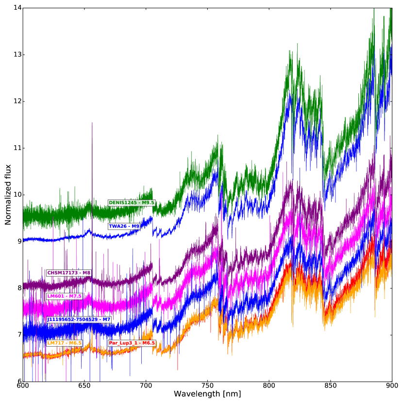
Figure 13: Spectra of Class III YSOs with spectral type later than M6 ordered according to their spectral type and normalized at 750 nm.