Small Area Quantile Estimation

Small Area Quantile Estimation

Abstract

Sample surveys are widely used to obtain information about totals, means, medians, and other parameters of finite populations. In many applications, similar information is desired for subpopulations such as individuals in specific geographic areas and socio-demographic groups. When the surveys are conducted at national or similarly high levels, a probability sampling can result in just a few sampling units from many unplanned subpopulations at the design stage. Cost considerations may also lead to low sample sizes from individual small areas. Estimating the parameters of these subpopulations with satisfactory precision and evaluating their accuracy are serious challenges for statisticians. To overcome the difficulties, statisticians resort to pooling information across the small areas via suitable model assumptions, administrative archives, and census data. In this paper, we develop an array of small area quantile estimators. The novelty is the introduction of a semiparametric density ratio model for the error distribution in the unit-level nested error regression model. In contrast, the existing methods are usually most effective when the response values are jointly normal. We also propose a resampling procedure for estimating the mean square errors of these estimators. Simulation results indicate that the new methods have superior performance when the population distributions are skewed and remain competitive otherwise.

1 Introduction

Sample surveys are widely used to obtain information about the totals, means, medians, and other parameters of finite populations. In many applications, the same information is desired for subpopulations such as individuals in specific geographic areas or in socio-demographic groups. The estimation of finite subpopulation parameters is referred to as the small area estimation problem (Rao 2003). While the geographic areas may not be small, there may be a shortage of direct information from individual areas. Often, the surveys are conducted at national or similarly high levels. The random nature of probability sampling can result in just a few sampling units from many unplanned subpopulations that are not considered at the design stage. Cost considerations can also lead to low sample sizes. Estimating the parameters of these subpopulations with satisfactory precision and evaluating their accuracy are serious challenges for statisticians.

Because of the scarcity of direct information from small areas, reliable estimates are possible only if indirect information from other areas is available and effectively utilized. This leads to a common thread of “borrowing strength.” Statisticians also seek auxiliary information from sources such as administrative archives and census data on subpopulations to obtain indirect estimates for the subpopulation parameter. These estimates may then be combined “optimally.”

The small area estimation problem has been intensively studied for many years. Early publications covering foundational work include Fay and Herriot (1979), Battese, Harter, and Fuller (1988), Prasad and Rao (1990), and Lahiri and Rao (1995). Successful applications can be found in Schaible (1993), Tzavidis et al. (2008), and Kriegler and Berk (2010). Elbers, Lanjouw, and Lanjouw (2003) use a unit-level model that combines census and survey data. The method has been employed by many to reveal the spatial distribution of poverty and income inequality (Haslett and Jones 2005; Neri, Ballini, and Betti 2005; Ballini, Betti, Carrette, and Neri 2006; Tarozzi and Deaton 2009). There are many papers containing novel developments in theory and methodology; see You and Rao (2002), Jiang and Lahiri (2006), Pfeffermann and Sverchkov (2007), Ghosh, Maiti, and Roy (2008), Jiang, Nguyen, and Rao (2010), Chaudhuri and Ghosh (2011), Marchetti, Tzavidis, and Pratesi (2012), Jiongo, Haziza, and Duchesne (2013), and Verret, Rao, and Hiridoglou (2015). We recommend Pfeffermann (2002, 2013), Rao (2003), and Rao and Molina (2015) as additional references.

In this paper, we develop an array of new small area quantile estimators. The existing methods such as that proposed by Molina and Rao (2010) utilize optimal prediction via the conditional expectation. This computation is most convenient when the response values are jointly normal. There are many ways to extend the approach to non-normal data, e.g., transforming the response to improve the fitness of the normal model or employing a skewed normal distribution to compute the optimal predictions. The novelty in our development is the introduction of a semiparametric density ratio model for the error distribution in the unit-level nested error regression model. We avoid restrictive parametric assumptions while “borrowing strength” between small areas. We also propose a resampling procedure to estimate the mean square errors of these estimators. Our simulation results indicate that the new methods have superior performance when the population distributions are skewed and remain competitive otherwise.

The paper is organized as follows. In Section 2, we review closely related developments. In Section 3, we introduce the new methods. In Section 4, we develop a resampling method for the estimation of the mean square errors. In Section 5, we give some theoretical results, leaving the technical proofs to the Appendix. In Section 6, we use simulation to reveal the properties of the new methods and compare them with existing methods using artificial data sets and a real data set. We end the paper with a summary and discussion.

2 Literature review

Let $\{(\mbox{\bf x}_{kj},y_{kj}):k=0,\ldots,m;j=1,\ldots,n_{k}\}$ be a random sample from a finite population with $m+1$ small areas where the $k$th area contains $N_{k}$ sampling units. We use $s_{k}$ to denote the set of observed sampling units in small area $k$. We refer to $\mbox{\bf x}_{kj}$ as an auxiliary variable. In some applications, all the $\mbox{\bf x}_{kj}$ values in the population are available from a census or register. In other applications, these values are known only for $j\in s_{k}$. Of course, the $y_{kj}$ are known only for $j\in s_{k}$. Estimation in both situations will be discussed. We also assume that the finite population and the observed sampling units can both be regarded as samples from a common probability model, i.e., the sampling plan is uninformative. The informative situation needs more careful treatment (Guadarrama, Molina, and Rao 2016).

We are interested in predicting finite-population parameter values under some model assumptions. Most finite-population parameters of interest have the following algebraic form:

$$H_{k}=N_{k}^{-1}\sum_{j=1}^{N_{k}}h(y_{kj})$$ (1)

for some known function $h(\cdot)$. When $h$ is chosen as $h(y)=y$, $H_{k}$ is the small area mean. When $h(y)=\mathbbm{1}(y\leq t)$ for some real value $t$, where $\mathbbm{1}(\cdot)$ is an indicator function, $H_{k}$ is the small area cumulative distribution function $F_{k}(t)$ at $t$. The small area quantile function is the inverse of $F_{k}(t)$. We refer to Molina and Rao (2010) for additional examples.

Under a probability model on the finite population, the minimum variance unbiased prediction (when feasible) of $H_{k}$ is given by

$$E(H_{k}|\mbox{sampled information})=N_{k}^{-1}\sum_{j=1}^{N_{k}}E\{h(y_{kj})|\mbox{sampled information}\}.$$

If the resulting conditional expectation contains unknown model parameters, the prediction will be constructed with the unknown parameters replaced by suitable estimates. This leads to the empirical best predictor(s) (EBP) of Molina and Rao (2010):

$$\hat{H}_{k}=N_{k}^{-1}\big{\{}\sum_{j\not\in s_{k}}\hat{h}_{kj}+\sum_{j\in s_{k}}h(y_{kj})\big{\}}$$ (2)

where $\hat{h}_{kj}$ is the predicted value of $h(y_{kj})$.

In applications, it can be difficult to identify $s_{k}$ from the finite population. Hence, we may use its census version

$$\hat{H}_{k}^{\mbox{\sc c}}=N_{k}^{-1}\sum_{j=1}^{N_{k}}\hat{h}_{kj}.$$ (3)

The EBP works well, but establishing its optimality can be a challenging task.

Once a concrete model is given, the abstract EBP becomes a practical solution. On the model front, the nested-error (unit level) regression model (NER) of Battese, Harter, and Fuller (1988) is widely adopted. Under this model,

$$y_{kj}=\mbox{\bf x}_{kj}^{\tau}\mbox{$\boldsymbol{\betaup}$}+\nu_{k}+\varepsilon_{kj},$$ (4)

where $\nu_{k}$ denotes an area-specific random effect and $\varepsilon_{kj}$ is random error. The homogeneous NER model assumptions include $\nu_{k}\sim N(0,\sigma_{v}^{2})$, $\varepsilon_{kj}\sim N(0,\sigma_{e}^{2})$, and they are independent of each other and the auxiliary variable $\mbox{\bf x}_{kj}$. Relaxing the homogeneity to a more flexible variance structure leads to the heterogeneous NER (HNER) of Jiang and Nguyen (2012). Relaxing the normality of the error distribution to a skewed normal distribution is discussed by Diallo and Rao (2016). Recent extensions include replacing $\mbox{\bf x}_{kj}^{\tau}\mbox{$\boldsymbol{\betaup}$}$ with a spline (Opsomer et al. 2008; Ranalli, Breidt, and Opsomer 2016). One may also transform $y_{kj}$ to make the normality assumption more appropriate (Molina and Rao 2010).

Under NER or HNER models, the regression coefficient $\boldsymbol{\betaup}$ is common across the small areas. Samples from all the areas contain its information. When the overall sample size $n=\sum_{k=0}^{m}n_{k}$ is large, a high precision estimator $\hat{}\mbox{$\boldsymbol{\betaup}$}$ is possible. Given the population means $\bar{\mbox{\bf X}}_{k}$, we get an indirect estimator $\hat{\bar{\mbox{\bf Y}}}_{k}=\bar{\mbox{\bf X}}_{k}^{\tau}\hat{}\mbox{$\boldsymbol{\betaup}$}$. It may be optimally combined with the regression estimator $\bar{y}_{k}+(\bar{\mbox{\bf X}}_{k}-\bar{\mbox{\bf x}}_{k})\hat{\mbox{$\boldsymbol{\betaup}$}}$ in obvious notation to get the so-called BLUP of small area mean $\bar{Y}_{k}$. The linear combination coefficient depends on whether the NER or HNER model is assumed (Jiang and Lahiri 2006; Jiang and Nguyen 2012).

Another general approach is via calibration or generalized regression (Estevao and Sárndal 2006; Pfeffermann 2013). Suppose $\hat{h}_{kj}$ predicting $h(y_{kj})$ is available for all the units in the finite population. A calibration predictor of $H_{k}$ is given by

$$\hat{H}_{k}=N_{k}^{-1}\sum_{j=1}^{N_{k}}\hat{h}_{kj}+N_{k}^{-1}\sum_{j\in s_{k}}w_{kj}\{h(y_{kj})-\hat{h}_{kj}\}$$ (5)

where the $w_{kj}$ are design weights to reduce the risk of bias caused by informative sampling plans, and $s_{k}$ denotes the sample of units selected from area $k$. Under a simple random sample without replacement plan or if the sampling plan is non-informative, we may use $w_{kj}=N_{k}/n_{k}$. Specifically, under linear models such as NER, $\hat{h}_{kj}$ is generally chosen to be $\mbox{\bf x}_{kj}^{\tau}\hat{}\mbox{$\boldsymbol{\betaup}$}$ leading to the generalized regression estimator (GREG); see Pfeffermann (2013). In this case, the calibration estimator improves the efficiency of sample mean $\bar{y}_{k}$ by calibrating the difference between $\bar{}\mbox{\bf x}_{k}$ and $\bar{}\mbox{\bf X}_{k}$. In nonlinear situations, this approach needs census information on $x$ and calibrates only the difference between two averages: $N_{k}^{-1}\sum_{j=1}^{N_{k}}\hat{h}_{kj}$ and $N_{k}^{-1}\sum_{j\in s_{k}}w_{kj}\hat{h}_{kj}$. Hence, it is not a good choice for the estimation of quantiles.

Another choice of $\hat{h}_{kj}$ is via the M-quantile (Breckling and Chambers 1988). A regression quantile relates the response variable $Y$ and some covariate x through the equation

$$P(Y\leq\mbox{\bf x}^{\tau}\mbox{$\boldsymbol{\betaup}$}_{q}|\mbox{\bf X}=\mbox{\bf x})=q$$

for each $q\in(0,1)$ and a $q$-dependent $\mbox{$\boldsymbol{\betaup}$}_{q}$; see Koenker and Bassett (1978). Let $\rho_{q}(t)=q\mathbbm{1}(t<0)+(1-q)\mathbbm{1}(t>0)$. Then $\mbox{$\boldsymbol{\betaup}$}_{q}$ is also a solution to

$$\min{\mathbb{E}}\{\rho_{q}(Y-\mbox{\bf X}^{\tau}\mbox{$\boldsymbol{\betaup}$})|\mbox{\bf X}\}.$$

By this statement, we have implicitly assumed that the solution to the above equation in $\boldsymbol{\betaup}$ does not depend on the value of X. When the model is valid, $\mbox{\bf x}^{\tau}\mbox{$\boldsymbol{\betaup}$}_{q}$ is the $q$th quantile of the conditional distribution of $Y$ given $\mbox{\bf X}=\mbox{\bf x}$. Clearly, $\mbox{\bf X}^{\tau}\mbox{$\boldsymbol{\betaup}$}_{q}$ is a robust description of the conditional distribution of $Y$. Breckling and Chambers (1988) propose the use of a generic $\rho_{q}(\cdot)$ function (say $\psi$) and call the resulting $\mbox{\bf X}^{\tau}\mbox{$\boldsymbol{\betaup}$}_{q}$ the M-quantile.

In the context of small area estimation, let $\hat{}\mbox{$\boldsymbol{\betaup}$}(q)=\hat{}\mbox{$\boldsymbol{\betaup}$}_{q}$ be the fitted M-quantile given $q\in(0,1)$. Note that it depends on $q$. For each unit $k,j$ in the sample, one may find a $q$ value such that

$$y_{kj}=\mbox{\bf x}_{kj}^{\tau}\hat{}\mbox{$\boldsymbol{\betaup}$}(q).$$

An approximation may be used when an exact solution does not exist. Denote the solution as $q_{kj}$. Chambers and Tzavidis (2006) suggest that the average $q_{k\cdot}=n_{k}^{-1}\sum_{j=1}^{n_{k}}q_{kj}$ reflects the general quantile information of area $k$. This leads to $\hat{y}_{kj}=\mbox{\bf x}_{kj}^{\tau}\hat{}\mbox{$\boldsymbol{\betaup}$}(q_{k\cdot})$, the predicted area-specific cumulative distribution function

$$\hat{F}_{k}(t)={N_{k}^{-1}}\big{[}\sum_{j\in s_{k}}\mathbbm{1}(y_{kj}\leq t)+\sum_{j\not\in s_{k}}\mathbbm{1}\{\mbox{\bf x}_{kj}^{\tau}\hat{}\mbox{$\boldsymbol{\betaup}$}(q_{k\cdot})\leq t\}\big{]},$$

and the resulting quantile predictions.

As pointed out by Tzavidis and Chambers (2005) and Tzavidis et al. (2008), from $F_{k}(t)$ to $\hat{F}_{k}(t)$ the difference between $\mathbbm{1}(\mbox{\bf x}_{kj}^{\tau}\mbox{$\boldsymbol{\betaup}$}+\epsilon_{kj}\leq t)$ and $\mathbbm{1}(\mbox{\bf x}_{kj}^{\tau}\mbox{$\boldsymbol{\betaup}$}\leq t)$ is ignored, which leads to a nondiminishing error even when $n_{k}\to\infty$. To overcome this pitfall, a new estimator/predictor following the approach of Chambers and Dunstan (1986) is proposed. Let $\hat{\epsilon}_{kj}=y_{kj}-\hat{y}_{kj}$ be the M-quantile residuals for $j\in s_{k}$ over $k=0,1,\ldots,m$, where $\hat{y}_{kj}=\mbox{\bf x}_{kj}^{\tau}\hat{}\mbox{$\boldsymbol{\betaup}$}(q_{k\cdot})$. For each small area, construct an empirical distribution

$$\hat{G}_{k}(t)=n_{k}^{-1}\sum_{j\in s_{k}}\mathbbm{1}(\hat{\epsilon}_{kj}\leq t).$$

The revised estimate of $F_{k}$ (Tzavidis et al. 2008) can be written

$$\hat{F}^{\mbox{\sc mq}}_{k}(t)=N_{k}^{-1}\big{\{}\sum_{j\in s_{k}}\mathbbm{1}(y_{kj}\leq t)+\sum_{j\not\in s_{k}}\hat{G}_{k}(t-\hat{y}_{kj})\big{\}}.$$ (6)

Note that we have written this estimator in the form of the EBP of Molina and Rao (2010). The approach may also be made outlier-robust (Chambers et al., 2011).

This paper provides a new approach to the prediction of small area quantiles.

3 The proposed approach

We assume the basic NER model structure (4) but allow a generic $G_{k}$ for the distribution of $\varepsilon$, the expectation of which is zero. Hence,

$${\mathbb{E}}\{\mathbbm{1}(y_{kj}\leq y)|\nu_{k},x_{kj}\}=G_{k}(y-\nu_{k}-\mbox{\bf x}_{kj}^{\tau}\mbox{$\boldsymbol{\betaup}$}).$$

Based on a random sample $s_{k}$ and when feasible, we predict $F_{k}(y)$ by

$$\tilde{F}_{k}(y)=n_{k}^{-1}\sum_{j\in s_{k}}G_{k}(y-\nu_{k}-\mbox{\bf x}_{kj}^{\tau}\mbox{$\boldsymbol{\betaup}$}-\delta_{k}),$$ (7)

with $\delta_{k}$ chosen to permit the shrinkage effect via random effect considerations.

When census information on $x$ is available, we follow the principle of EBP (Molina and Rao 2010) to predict $F_{k}(y)$ by

$$\tilde{F}^{\mbox{\sc eb}1}_{k}(y)=N_{k}^{-1}\big{\{}\sum_{j\not\in s_{k}}G_{k}(y-\nu_{k}-\mbox{\bf x}_{kj}^{\tau}\mbox{$\boldsymbol{\betaup}$})+\sum_{j\in s_{k}}\mathbbm{1}(y_{kj}\leq y)\big{\}}.$$

If the identification of $s_{k}$ is difficult, then the following predictor is just as effective:

$$\tilde{F}^{\mbox{\sc eb}2}_{k}(y)=N_{k}^{-1}\sum_{j=1}^{N_{k}}G_{k}(y-\nu_{k}-\mbox{\bf x}_{kj}^{\tau}\mbox{$\boldsymbol{\betaup}$}).$$

Since $\nu_{k}$, $\boldsymbol{\betaup}$, and $G_{k}$ are not known in applications in general, it is common practice to replace them in the above expressions by their predictions/estimates. This leads to a variety of predictors. Let $\hat{F}_{k}(y)$ be a generic predictor of the small area distribution. The corresponding small area quantiles predictor will be defined as

$$\hat{\xi}_{k}=\hat{\xi}_{k,\alpha}=\inf\{y:\hat{F}_{k}(y)\geq\alpha\}$$ (8)

for any $\alpha\in(0,1)$. The remaining tasks are to choose $\delta_{k}$, estimate $G_{k}$, and predict the other quantities.

3.1 Estimation under the NER model

Under NER, we can estimate the unknown parameters via the maximum likelihood. Let $\tilde{\sigma}^{2}$, $\tilde{\sigma}_{v}^{2}$, and $\tilde{}\mbox{$\boldsymbol{\betaup}$}$ be the MLEs. An established small area mean estimate is the empirical BLUP (EBLUP) given by

$$\tilde{\bar{Y}}_{k}=\bar{\mbox{\bf X}}_{k}^{\tau}\tilde{}\mbox{$\boldsymbol{\betaup}$}+\tilde{\gamma}_{k}(\bar{y}_{k}-\bar{\mbox{\bf x}}_{k}^{\tau}\tilde{}\mbox{$\boldsymbol{\betaup}$})=\bar{\mbox{\bf X}}_{k}^{\tau}\tilde{}\mbox{$\boldsymbol{\betaup}$}+\tilde{\gamma}_{k}\tilde{\nu}_{k}$$ (9)

where $\tilde{\gamma}_{k}=n_{k}\tilde{\sigma}_{v}^{2}/(\tilde{\sigma}^{2}+n_{k}\tilde{\sigma}_{v}^{2})$ and $\tilde{\nu}_{k}=\bar{y}_{k}-\bar{\mbox{\bf x}}_{k}^{\tau}\tilde{}\mbox{$\boldsymbol{\betaup}$}$. Note that the EBLUP has shrunk $\tilde{v}_{k}$ toward zero by modeling $v_{k}$ as a random effect. Let $\delta_{k}=\tilde{\bar{Y}}_{k}-\bar{\mbox{\bf x}}_{k}^{\tau}\tilde{}\mbox{$\boldsymbol{\betaup}$}$ in (7); we then get a predictor as

$$\hat{F}^{\mbox{\sc ner}}_{k}(y)=\frac{1}{n_{k}}\sum_{j=1}^{n_{k}}\Phi\left(\{y-(\mbox{\bf x}_{kj}-\bar{}\mbox{\bf x}_{k})^{\tau}\tilde{}\mbox{$\boldsymbol{\betaup}$}-\tilde{\bar{Y}}_{k}\}/\tilde{\sigma}_{e}\right).$$ (10)

The mean of the distribution $\hat{F}^{\mbox{\sc ner}}_{k}(y)$ is exactly $\tilde{\bar{Y}}_{k}$ because of the choice of $\delta_{k}$.

When the census $x$ information is available, the EBP versions of $\hat{F}^{\mbox{\sc ner}}_{k}(y)$ are given by

$$\hat{F}^{\mbox{\sc eb}1}_{k}(y)=N_{k}^{-1}\big{\{}\sum_{j\not\in s_{k}}\Phi(\{y-\tilde{\nu}_{k}-\mbox{\bf x}_{kj}^{\tau}\tilde{}\mbox{$\boldsymbol{\betaup}$}\}/\tilde{\sigma}_{e})+\sum_{j\in s_{k}}\mathbbm{1}(y_{kj}\leq y)\big{\}}$$ (11)

and

$$\hat{F}^{\mbox{\sc eb}2}_{k}(y)=N_{k}^{-1}\sum_{j=1}^{N_{k}}\Phi(\{y-\tilde{\nu}_{k}-\mbox{\bf x}_{kj}^{\tau}\tilde{}\mbox{$\boldsymbol{\betaup}$}\}/\tilde{\sigma}_{e}).$$ (12)

3.2 Estimation under DRM

As pointed out by Diallo and Rao (2016), the normality assumption on the error distribution of $\varepsilon$ can have a marked influence on the estimation of $F_{k}$. To alleviate this concern, a skewed normal distribution can be used. In this paper, we adopt a semiparametric density ratio model (DRM) for $G_{k}$ (Anderson 1979):

$$\log\{dG_{k}(t)/dG_{0}(t)\}=\mbox{$\boldsymbol{\thetaup}$}_{k}^{\tau}\mbox{\bf q}(t),$$ (13)

with a prespecified $d_{2}$-variate function $\mbox{\bf q}(t)$ and area-specific tilting parameter $\mbox{$\boldsymbol{\thetaup}$}_{k}$. We require the first element of $\mbox{\bf q}(t)$ to be one so that the first element of $\mbox{$\boldsymbol{\thetaup}$}_{k}$ is a normalization parameter. The baseline distribution $G_{0}(t)$ is left unspecified, and there many potential choices of $\mbox{\bf q}(t)$. The nonparametric $G_{0}$ has abundant flexibility while the parametric tilting factor $\mbox{$\boldsymbol{\thetaup}$}_{k}^{\tau}\mbox{\bf q}(t)$ enables effective “strength borrowing” between small areas. Note also that any $G_{j}$, not just $G_{0}$, may be regarded as a baseline distribution because

$$\log\{dG_{k}(t)/dG_{j}(t)\}=(\mbox{$\boldsymbol{\thetaup}$}_{k}-\mbox{$\boldsymbol{\thetaup}$}_{j})^{\tau}\mbox{\bf q}(t).$$ (14)

DRM is flexible, as testified by its inclusion of the normal, Gamma, and many other distribution families. Under this model assumption, we look for an estimate of $G_{k}$.

Estimating $G_{k}$ under DRM.

Consider an artificial situation where we have $m+1$ samples $\{\varepsilon_{kj}:j=1,2,\ldots,n_{k};k=0,\ldots,m\}$ from a DRM. Following Owen (1988, 2001) or Qin and Lawless (1994), we confine the form of the candidate $G_{0}$ to $G_{0}(t)=\sum_{k,j}p_{kj}\mathbbm{1}(\varepsilon_{kj}\leq t)$, and the summation $\sum_{k,j}$ is short for $\sum_{k=0}^{m}\sum_{j=1}^{n_{k}}$. The support of $G_{0}$ includes all $\varepsilon_{kj}$, not just those with $k=0$. This is part of the strength-borrowing strategy. In this setting, $p_{kj}=dG_{0}(\varepsilon_{kj})$ and $dG_{k}(\varepsilon_{ij})=p_{ij}\exp\{\mbox{$\boldsymbol{\thetaup}$}_{k}^{\tau}\mbox{\bf q}(\varepsilon_{ij})\},\;k=0,1,\ldots,m,$ where $\mbox{$\boldsymbol{\thetaup}$}_{k}$ are $d_{2}$-variate unknown parameters, and

$$G_{k}(t)=\sum_{i,j}p_{ij}\exp\{\mbox{$\boldsymbol{\thetaup}$}_{k}^{\tau}\mbox{\bf q}(\varepsilon_{ij})\}\mathbbm{1}(\varepsilon_{ij}\leq t).$$ (15)

Clearly, $\mbox{$\boldsymbol{\thetaup}$}_{0}=0$ when $G_{0}$ is chosen as the baseline. Because $\varepsilon_{kj}$ follows $G_{k}(t)$, it contributes to the likelihood only through $dG_{k}(\varepsilon_{kj})$. This leads to the empirical likelihood (EL):

$$L_{n}(G_{0},G_{1},\ldots,G_{m})=\prod_{k,j}dG_{k}(\varepsilon_{kj})=\big{(}\prod_{k,j}p_{kj}\big{)}\cdot\exp\big{[}\sum_{k,j}\{\mbox{$\boldsymbol{\thetaup}$}_{k}^{\tau}\mbox{\bf q}(\varepsilon_{kj})\}\big{]}$$

where the $p_{kj}$’s satisfy $p_{kj}\geq 0$ and for all $k=0,1,\ldots,m$,

$$\sum_{i,j}p_{ij}\exp\{\mbox{$\boldsymbol{\thetaup}$}_{k}^{\tau}\mbox{\bf q}(\varepsilon_{ij})\}=1.$$ (16)

Let $\mbox{$\boldsymbol{\thetaup}$}^{\tau}=(\mbox{$\boldsymbol{\thetaup}$}^{\tau}_{1},\ldots,\mbox{$\boldsymbol{\thetaup}$}_{m}^{\tau})$. Maximizing the empirical log-likelihood

$$\ell_{n}(\mbox{$\boldsymbol{\thetaup}$},G_{0})=\sum_{k,j}p_{kj}+\sum_{k,j}\{\mbox{$\boldsymbol{\thetaup}$}_{k}^{\tau}\mbox{\bf q}(\varepsilon_{kj})\}$$

with respect to $G_{0}$ under constraints (16) results in the fitted probabilities (Qin and Lawless 1994)

$$\hat{p}_{kj}=n^{-1}\{1+\sum_{l=1}^{m}\lambda_{l}[\exp\{\mbox{$\boldsymbol{\thetaup}$}_{l}^{\tau}\mbox{\bf q}(\varepsilon_{kj})\}-1]\}^{-1}$$ (17)

and the profile EL, up to an additive constant,

$$\tilde{\ell}_{n}(\mbox{$\boldsymbol{\thetaup}$})=-\sum_{k,j}\log\{1+\sum_{l=1}^{m}\lambda_{l}[\exp\{\mbox{$\boldsymbol{\thetaup}$}_{l}^{\tau}\mbox{\bf q}(\varepsilon_{kj})\}-1]\}+\sum_{k,j}\{\mbox{$\boldsymbol{\thetaup}$}_{k}^{\tau}\mbox{\bf q}(\varepsilon_{kj})\}$$

with $(\lambda_{1},\lambda_{2},...,\lambda_{m})$ being the solution to

$$\sum_{i,j}\frac{\exp\{\mbox{$\boldsymbol{\thetaup}$}_{k}^{\tau}\mbox{\bf q}(\varepsilon_{ij})\}-1}{1+\sum_{l=1}^{m}\lambda_{l}[\exp\{\mbox{$\boldsymbol{\thetaup}$}_{l}^{\tau}\mbox{\bf q}(\varepsilon_{ij})\}-1]}=0$$

for $k=1,\ldots,m$. The stationary points of $\tilde{\ell}_{n}(\mbox{$\boldsymbol{\thetaup}$})$ coincide with those of a dual form of the empirical log-likelihood function (Keziou and Leoni-Aubin 2008)

$$\breve{\ell}_{n}(\mbox{$\boldsymbol{\thetaup}$})=-\sum_{k,j}\log\big{[}\sum_{r=0}^{m}\rho_{r}\exp\{\mbox{$\boldsymbol{\thetaup}$}_{r}^{\tau}\mbox{\bf q}(\varepsilon_{kj})\}\big{]}+\sum_{k,j}\mbox{$\boldsymbol{\thetaup}$}_{k}^{\tau}\mbox{\bf q}(\varepsilon_{kj}),$$ (18)

with $\rho_{r}=n_{r}/n$, $r=0,1,\ldots,m$.

For point estimation, it is simpler to work with $\breve{\ell}_{n}(\mbox{$\boldsymbol{\thetaup}$})$, which is convex and free from constraints. Once the values of $\varepsilon_{kj}$ are provided, it is relatively simple to find its maximum point, which is the maximum EL estimate of $\boldsymbol{\thetaup}$. We then use (17) to compute the fitted values with $\lambda_{l}$ replaced by $\rho_{l}$. We subsequently obtain $\hat{G}_{k}$ and the other parameters of interest via the invariance principle.

This line of approach first appeared in Qin and Zhang (1997), Qin (1998), Zhang (1997), and others. In particular, the properties of the quantile estimators are discussed by Zhang (2000) and Chen and Liu (2013). In the current application, we use $\hat{\varepsilon}_{kj}$, given below in (20), for the computation.

Parameter estimation with fitted residuals

Suppose we have a sample $(y_{kj},\mbox{\bf x}_{kj})$ for $k=0,1,\ldots,m$ and $j=1,\ldots,n_{k}$ satisfying the NER with the error distribution from the DRM. We first eliminate the random effect $\nu_{k}$ from the NER by centralizing both sides of (4), which leads to

$$y_{kj}-\bar{y}=(\mbox{\bf x}_{kj}-\bar{}\mbox{\bf x}_{k})^{\tau}\mbox{$\boldsymbol{\betaup}$}+\varepsilon_{kj}-\bar{\varepsilon}_{k},$$

where ${\bar{}\mbox{\bf x}}_{k}$ and $\bar{y}_{k}$ are the sample means over small area $k$. The least squares estimator of $\boldsymbol{\betaup}$ under the centralized model is

$$\hat{}\mbox{$\boldsymbol{\betaup}$}=\{\sum_{k,j}(\mbox{\bf x}_{kj}-{\bar{}\mbox{\bf x}}_{k})^{\tau}(\mbox{\bf x}_{kj}-{\bar{}\mbox{\bf x}}_{k})\}^{-1}\{\sum_{k,j}(\mbox{\bf x}_{kj}-{\bar{}\mbox{\bf x}}_{k})^{\tau}(y_{kj}-\bar{y}_{k})\}.$$ (19)

The residuals of this fit are given by

$$\hat{\varepsilon}_{kj}=y_{kj}-\bar{y}_{k}-(\mbox{\bf x}_{kj}-\bar{}\mbox{\bf x}_{k})^{\tau}\hat{}\mbox{$\boldsymbol{\betaup}$}.$$ (20)

We then treat $\{\hat{\varepsilon}_{kj}:j=1,2,\ldots,n_{k}\}$ as samples from the DRM and apply the EL method of Section 3.2.

Let $\ell_{n}(\mbox{$\boldsymbol{\thetaup}$})$ denote the log EL function (18) with $\varepsilon_{kj}$ replaced by $\hat{\varepsilon}_{kj}$. We define the maximum EL estimator of $\boldsymbol{\thetaup}$ by $\hat{}\mbox{$\boldsymbol{\thetaup}$}={\mbox{argmax}}\ell_{n}(\mbox{$\boldsymbol{\thetaup}$})$ and accordingly define the estimators

$$\hat{G}_{k}(t)=\sum_{i,j}\hat{p}_{ij}\exp\{\hat{\mbox{$\boldsymbol{\thetaup}$}}_{k}^{\tau}\mbox{\bf q}(\hat{\varepsilon}_{ij})\}\mathbbm{1}(\hat{\varepsilon}_{ij}<t)$$ (21)

with $\hat{}\mbox{$\boldsymbol{\thetaup}$}_{0}=\mbox{\bf 0}$ by convention and $\hat{p}_{ij}=n^{-1}\{1+\sum_{l=1}^{m}\rho_{l}[\exp\{{\hat{\mbox{$\boldsymbol{\thetaup}$}}_{l}^{\tau}}\mbox{\bf q}(\hat{\varepsilon}_{ij})\}-1]\}^{-1}.$ Consequently, after targeting the small area mean estimate in (10), we estimate $F_{k}(y)$ by

$$\hat{F}^{\mbox{\sc el}}_{k}(y)=\frac{1}{n_{k}}\sum_{j=1}^{n_{k}}\hat{G}_{k}\left(y-(\mbox{\bf x}_{kj}-\bar{}\mbox{\bf x}_{k})^{\tau}\hat{}\mbox{$\boldsymbol{\betaup}$}-\tilde{\bar{Y}}_{k}\right)$$ (22)

where $\tilde{\bar{Y}}_{k}$ is given in (9). When the census $x$ information is available, the EBP versions are

$$\hat{F}^{\mbox{\sc ebel}1}_{k}(y)=N_{k}^{-1}\big{\{}\sum_{j\not\in s_{k}}\hat{G}_{k}(y-\hat{\nu}_{k}-\mbox{\bf x}_{kj}^{\tau}\hat{}\mbox{$\boldsymbol{\betaup}$})+\sum_{j\in s_{k}}\mathbbm{1}(y_{kj}\leq y)\big{\}}$$ (23)

where $\hat{\nu}_{k}=\bar{y}_{k}-\bar{\mbox{\bf x}}_{k}^{\tau}\hat{}\mbox{$\boldsymbol{\betaup}$}$, and

$$\hat{F}^{\mbox{\sc ebel}2}_{k}(y)=N_{k}^{-1}\sum_{j=1}^{N_{k}}\hat{G}_{k}(y-\hat{\nu}_{k}-\mbox{\bf x}_{kj}^{\tau}\hat{}\mbox{$\boldsymbol{\betaup}$}).$$ (24)

The quantiles are estimated accordingly.

4 Variance/MSE estimation

When an estimator is assembled in many steps, its variance is often too complex to be analytically evaluated. Resampling the variance estimation becomes a good choice (Molina and Rao 2010). Based on whether or not census information is available and whether the error distribution is regarded as $N(0,\sigma_{e}^{2})$ under the NER or $G_{k}$ under the DRM, we have four distinct small area quantile estimators. We give a detailed description of a resampling method for the case where census information is available and the error distributions $G_{k}$ satisfy the DRM. We then give a simple description of the changes needed for the other three estimators.

Our resampling procedure is as follows:

1. Under the NER model, obtain the maximum likelihood estimates $\tilde{\sigma}_{v}^{2}$ and $\tilde{\sigma}_{e}^{2}$, and compute $\tilde{\bar{Y}}_{k}$.

2. Calculate $\hat{}\mbox{$\boldsymbol{\betaup}$}$ and obtain $\hat{}\mbox{$\boldsymbol{\thetaup}$}_{k}$ and $\hat{G}_{k}$ as in (21) under DRM.

3. For $b=1,\ldots,B$ over $k,j$ with $B$ large, generate

   $$\nu_{k}^{*(b)}\sim N(0,\tilde{\sigma}_{v}^{2})~{}\mbox{and}~{}e_{kj}^{*(b)}\sim\hat{G}_{k}.$$

4. Construct $B$ (conditionally) independent and identically distributed (iid) bootstrap populations with

   $$y_{kj}^{*(b)}=\mbox{\bf x}_{kj}^{\tau}\hat{}\mbox{$\boldsymbol{\betaup}$}+\nu_{k}^{*(b)}+e_{kj}^{*(b)}$$

   for $j=1,\ldots,N_{k}$ and $k=0,1,\ldots,m$.

5. For each bootstrap sample, compute

   $$F^{*(b)}_{k}(t)=N_{k}^{-1}\sum_{j=1}^{N_{k}}\mathbbm{1}(y_{kj}^{*(b)}\leq t)$$

   and the corresponding $\hat{F}^{*(b)}_{k}(t)$ as in (24).

6. For any parameter that can be written in the form of $H(F_{k})$, compute the bootstrap mean square error estimator of MSE($H(\hat{F}_{k})$) via

   $$\mbox{mse}(H(\hat{F}_{k}))=\frac{1}{B}\sum_{b=1}^{B}\{H(\hat{F}_{k}^{*(b)})-H(F_{k}^{*(b)})\}^{2}.$$ (25)

Sampling from $\hat{G}_{k}$ can easily be done with existing R functions because it is a discrete distribution on $\hat{\epsilon}_{ij}$ with probabilities $\hat{p}_{ij}\exp\{\hat{}\mbox{$\boldsymbol{\thetaup}$}_{k}\mbox{\bf q}(\hat{\varepsilon}_{ij})\}$. Note that the support is over all the fitted residuals, not just those in small area $k$.

Under the NER, we replace $\hat{G}_{k}$ in Step 3 by $N(0,\tilde{\sigma}_{e}^{2})$. Under the DRM without census information, we generate $\epsilon_{kj}$ in Step 3 only for $j\in s_{k}$ and in Step 6 we use the sample variance of $H(\hat{F}_{k}^{*(b)})-H(F_{k}^{*(b)})$ instead of the squared average.

5 Asymptotic properties

For each $k$, the covariates $\{\mbox{\bf x}_{kj},j=1,2,\ldots,n_{k}\}$ are iid with finite mean and nonsingular and finite covariance matrix $\mbox{\bf V}_{k}$; the error terms $\{\varepsilon_{kj}:j=1,2,\cdots,n_{k}\}$ are iid samples, independent of the covariates, with conditional variance $\sigma^{2}_{k}$. The pure residuals $\varepsilon_{kj}$ form $m+1$ samples from populations with the distribution function $G_{k}$ satisfying (13). Let the total sample size $n=\sum_{k}n_{k}\to\infty$, and assume $\rho_{k}=n_{k}/n$ remains a constant (or within an $n^{-1}$ range) as $n$ increases. Let $\hat{}\mbox{$\boldsymbol{\betaup}$}$ and $\hat{}\mbox{$\boldsymbol{\thetaup}$}$ be defined by (19) and the subsequent steps.

Theorem 1.

Assume the general setting presented in this subsection. Let $\mbox{\bf V}_{x}=\sum_{k=0}^{m}\rho_{k}\mbox{\bf V}_{k}$. As $n\rightarrow\infty$, we have $\sqrt{n}(\hat{}\mbox{$\boldsymbol{\betaup}$}-\mbox{$\boldsymbol{\betaup}$})\overset{d}{\longrightarrow}N(0,\mbox{$\mathbf{\Sigma}$}_{\mbox{$\boldsymbol{\betaup}$}}),$ where $\overset{d}{\longrightarrow}$ denotes convergence in distribution and $\mbox{$\mathbf{\Sigma}$}_{\mbox{$\boldsymbol{\betaup}$}}=\mbox{\bf V}_{x}^{-1}(\sum_{k}\rho_{k}\mbox{\bf V}_{k}\sigma_{k}^{2})\mbox{\bf V}_{x}^{-1}$.

For ease of exposition of the next theorem, we introduce some notation. For $k=0,1,\ldots,m$, let

$$h(x;\mbox{$\boldsymbol{\thetaup}$})=\sum_{k=0}^{m}\rho_{k}\exp\{\mbox{$\boldsymbol{\thetaup}$}_{k}^{\tau}\mbox{\bf q}(x)\};~{}~{}~{}h_{k}(x;\mbox{$\boldsymbol{\thetaup}$})=\rho_{k}\exp\{\mbox{$\boldsymbol{\thetaup}$}_{k}^{\tau}\mbox{\bf q}(x)\}/h(x;\mbox{$\boldsymbol{\thetaup}$}).$$

Clearly, $0<h_{k}<1$ for all $k$. Let $\mbox{\bf h}(x;\mbox{$\boldsymbol{\thetaup}$})=\{h_{0}(x;\mbox{$\boldsymbol{\thetaup}$}),\ldots,h_{m}(x;\mbox{$\boldsymbol{\thetaup}$})\}^{\tau}$ and define an $(m+1)\times(m+1)$ matrix

$$\mbox{\bf H}(x;\mbox{$\boldsymbol{\thetaup}$})=\mbox{diag}\{\mbox{\bf h}(x;\mbox{$\boldsymbol{\thetaup}$})\}-\mbox{\bf h}(x;\mbox{$\boldsymbol{\thetaup}$})\mbox{\bf h}^{\tau}(x;\mbox{$\boldsymbol{\thetaup}$}).$$

We will use $h(x;\overset{\sqbullet}{x})$ and $h(x;\overset{\sqbullet}{\mbox{$\boldsymbol{\thetaup}$}})$ for the partial derivatives of $h$ with respect to $x$ and $\boldsymbol{\thetaup}$ respectively. When $\mbox{$\boldsymbol{\thetaup}$}=\mbox{$\boldsymbol{\thetaup}$}^{*}$, the true value of $\boldsymbol{\thetaup}$, we may drop $\mbox{$\boldsymbol{\thetaup}$}^{*}$ in $h(x;\mbox{$\boldsymbol{\thetaup}$}^{*})$ and denote it as $h(x)$. Lastly, we use $d\bar{G}(x)$ for $h(x;\mbox{$\boldsymbol{\thetaup}$}^{*})dG_{0}(x)$ in the integrations.

Theorem 2.

Assume the conditions of Theorem 1. Furthermore, assume the population distributions $G_{k}$ satisfy the DRM (13) with the true parameter value $\mbox{$\boldsymbol{\thetaup}$}^{*}$, and $\int h(t;\mbox{$\boldsymbol{\thetaup}$})dG_{0}<\infty$ in a neighborhood of $\mbox{$\boldsymbol{\thetaup}$}^{*}$. Assume the components of $\mbox{\bf q}(t)$ are linearly independent with the first element being one, twice differentiable, and that there exist a function $\psi(t)$ and $c_{0}>0$ such that

$$\sup_{t:|t-u|\leq c_{0}}\{\|\mbox{\bf q}(t)\|\|{\mbox{\bf q}}(\overset{\sqbullet\sqbullet}{t})\|+\|\mbox{\bf q}(t)\|\|{\mbox{\bf q}}(\overset{\sqbullet}{t})\|^{2}\}\leq\psi(u)$$ (26)

for all $u$ with $\int\psi(u)d\bar{G}(u)<\infty$. Then as $n$ goes to infinity, $\sqrt{n}(\hat{}\mbox{$\boldsymbol{\thetaup}$}-\mbox{$\boldsymbol{\thetaup}$}^{*})\overset{d}{\longrightarrow}N(\mbox{\bf 0},\mbox{$\mathbf{\Omega}$})$ where $\mathbf{\Omega}$ is given in (A.10) in the supplementary material.

The assumption that $\int h(t;\mbox{$\boldsymbol{\thetaup}$})dG_{0}(t)<\infty$ in a neighborhood of $\mbox{$\boldsymbol{\thetaup}$}^{*}$ implies the existence of the moment generating function of $\mbox{\bf q}(t)$ and therefore all its finite moments.

We next examine the asymptotic properties of the proposed small area quantile estimators, which we call EL quantiles for short.

Theorem 3.

Assume the conditions of Theorem 2. Suppose in addition that the $G_{k}(t)$ have smooth and bounded density functions, and $F_{k}(y)$ has positive density at $\xi_{k}$. Then the EL quantile (8) based on (22) is root-$n$ consistent. That is, $\hat{\xi}_{k}-\xi_{k}=O_{p}(n^{-1/2})$.

6 Simulation study

In this section, we investigate the performance of various small area quantile estimators and their variance estimates. In the simulation, we examine the $5\%$, $25\%$, $50\%$, $75\%$, and $95\%$ small area quantile estimations.

6.1 Simulation settings

The first task of the simulation is to create finite populations. We consider the following model for the general structure of the population:

$$y_{kj} = \mbox{\bf x}_{kj}^{\tau}\mbox{$\boldsymbol{\betaup}$}+\nu_{k}+\varepsilon_{kj}.$$ (27)

For authenticity, we use real survey data as a blueprint to design the following simulation populations:

1. For each $k=0,1,\ldots 19$, generate $N_{k}=1000$ three-dimensional $\mbox{\bf x}_{kj}=(x_{kj1},x_{kj2},x_{kj3})$ values, where $x_{kj1}\sim U(0,50)$, $x_{kj2}=50z_{kj}$, $z_{kj}\sim Beta(0.6,0.6)$, and conditional $x_{kj3}|z_{kj}\sim\mbox{Binom}(12,\;0.6+0.1x_{kj2})$.

2. Let $\mbox{$\boldsymbol{\betaup}$}_{0}^{\tau}=(0.019,0.022,0.074)$.

3. Generate $\nu_{k}$ from $N(8,1)$.

For the error distribution, we generate $\varepsilon_{kj}$ from

• (i) $N(0,\sigma_{e}^{2})$ with $\sigma_{e}^{2}=2$;

• (ii) normal mixture $0.5N(-\mu_{k}/6,1)+0.5N(\mu_{k}/6,1)$;

• (iii) normal mixture $0.1N(-\mu_{k}/2,1)+0.9N(\mu_{k}/18,1)$;

• (iv) normal mixture $0.9N(-\mu_{k}/18,1)+0.1N(\mu_{k}/2,1)$.

A single error distribution chosen from the above is applied to all the small areas. Each of them either (i) satisfies the NER model assumption; (ii) is non-normal but symmetric; (iii) is skewed to the right; or (iv) is skewed to the left.

We generate $\mu_{k}$ in (ii)–(iv) from the uniform distribution on the interval $[4.5,6]$ to determine the impact of mildly different error distributions in different small areas.

6.2 Predictors in the simulation

We study the performance of seven representative quantile predictors. Their corresponding area population distribution predictors are as follows.

1. Direct Predictor (DIR): we compute the sample quantiles for small area $k$ based on the sampled response values $y_{kj}$.

2. The NER-based predictor (NER): This predictor $\hat{F}^{\mbox{\sc ner}}_{k}(y)$ is defined in (10) assuming that the error distribution is normal. It uses only sampled $x$ information and the known population mean $\bar{\mbox{\bf X}}_{k}$ for each small area.

3. The EL-based predictor (EL): This predictor $\hat{F}^{\mbox{\sc el}}_{k}(y)$ is defined in (22). It uses only sampled $x$ information and the known subpopulation mean $\bar{}\mbox{\bf X}_{k}$ of each small area.

4. The NER-based census predictor (EB): This predictor $\hat{F}^{\mbox{\sc eb}2}_{k}(y)$ is defined in (12) assuming that the error distribution is normal. The other predictor $\hat{F}^{\mbox{\sc eb}1}_{k}(y)$ leads to nearly identical performance for the quantile estimation. To save space, $\hat{F}^{\mbox{\sc eb}1}_{k}(y)$ is not included in the simulation.

5. The proposed census predictor $\hat{F}^{\mbox{\sc ebel}2}_{k}(y)$ (EBEL): This estimator is given in (24). It is an analog of $\hat{F}^{\mbox{\sc eb}2}_{k}(y)$ except for using an EL-DRM-based estimate of the error distribution in the linear-model setting.

6. The EBP of Molina and Rao (MR): This is the predictor specified in (2) under the NER model. Additional implementation details are given below. The conditional distribution of $y_{kj}$ given sample $s_{k}$ can be expressed as

   $$y_{kj|s}=\mu_{kj|s}+u_{k}+\epsilon_{kj}$$ (28)

   with the conditional mean $\mu_{kj|s}=\mbox{\bf x}_{kj}\mbox{$\boldsymbol{\betaup}$}+\gamma_{k}(\bar{y}_{k}-\mbox{\bf x}_{k}^{\tau}\mbox{$\boldsymbol{\betaup}$})$, area-specific conditional random effect $u_{k}\sim N(0,(1-\gamma_{i})\sigma_{v}^{2})$, and conditional residual error $\epsilon_{kj}\sim N(0,\sigma_{e}^{2})$. The nonrandom constants and unknown parameter values of $\gamma_{k}$, $\sigma_{v}^{2}$, $\sigma_{e}^{2}$ are replaced by their estimated values (MLE in our simulation) in the computation. With this preparation, we generate $y_{kj}^{(\ell)}$ for each $j\not\in s_{k}$ according to (28) for $\ell=1,2,\ldots,L=100$. The corresponding empirical distribution

   $$\hat{F}_{kj|s}(t)=L^{-1}\sum_{\ell=1}^{L}\mathbbm{1}(y_{kj}^{(\ell)}\leq t)$$

   is used to form the predictor

   $$\hat{F}_{k}^{\mbox{\sc mr}}(t)=N_{k}^{-1}\big{\{}\sum_{j\not\in s_{k}}\hat{F}_{kj|s}(t)+\sum_{j\in s_{k}}\mathbbm{1}(y_{kj}\leq t)\big{\}}$$ (29)

   and the corresponding quantile predictions.

7. The M-quantile predictor (MQ): this predictor is specified in (6), and it is also a census predictor. Additional implementation details must be specified. We use

   $$\psi(u;q)=q\mathbbm{1}(u>0)-(1-q)\mathbbm{1}(u\leq 0)$$

   for $q\in(0,1)$. For each $q=\{1,\ldots,199\}/200$ and small area $k$, we search for a solution in $\boldsymbol{\betaup}$ to

   $$\sum_{j\in s_{k}}\psi(y_{kj}-\mbox{\bf x}_{kj}^{\tau}\mbox{$\boldsymbol{\betaup}$};q)\mbox{\bf x}_{kj}^{\tau}=0.$$

   Denote the solution as $\hat{}\mbox{$\boldsymbol{\betaup}$}_{k}(q)$. For each $y_{kj}\in s_{k}$, we find a q-value in $\{1,\ldots,199\}/200$ that minimizes $|y_{kj}-\mbox{\bf x}_{kj}\hat{}\mbox{$\boldsymbol{\betaup}$}_{k}(q)|$, and this gives us $q_{kj}$. The other numerical details have been given earlier.

We do not include the method of Elbers, Lanjouw, and Lanjouw (2003) because it is not designed specifically for small area quantile estimation, and its properties have been well investigated by Molina and Rao (2010). We exclude from the simulation some of the other predictors discussed in this paper. Preliminary experiments indicated that they did not outperform the predictors that we have included.

One must specify $\mbox{\bf q}(t)$ in the EL-DRM-based estimators (EL2, EBEL2). There are many reasonable candidates, and after some experiments, we settled on $\mbox{\bf q}(t)=(1,\mbox{sign-root}(t))^{\tau}$. It is not uniformly the best choice. To reduce the amount of computation, we included only this choice in our simulation. In applications, mild model violation is unavoidable. This choice is motivated by its overall performance in terms of “model robustness.”

The seven predictors listed above form two groups: the first group does not use census $x$ information and the second group does. Their performance will be judged in light of this difference.

6.3 Performance measures

Let ${\hat{\xi}}_{k}^{(j)}$ and ${{\xi}}_{k}^{(j)}$denote a generic quantile estimate in the $j$th repetition and the corresponding population quantile. We report the average mean squared error (amse), defined to be:

$${\mbox{\sc amse}}=\{N(m+1)\}^{-1}\sum_{k=0}^{m}\sum_{j=1}^{N}({\hat{\xi}_{k}^{(j)}}-\xi_{k}^{(j)})^{2}.$$

This combines the loss of precision due to bias and variation; it is a convenient metric of the performance of different estimation methods. We find that using both variance and bias does not lead to more detailed performance information but makes the judgement burdensome.

6.4 Simulation results

We generate a new finite population for each simulation replication. The small area population quantiles therefore vary from replication to replication, which is necessary for assessing the performance of the model-based methods.

We provide simulated amse values of all the methods for the populations generated with $\mbox{$\boldsymbol{\betaup}$}=1.0\mbox{$\boldsymbol{\betaup}$}_{0},1.25\mbox{$\boldsymbol{\betaup}$}_{0}$, and $1.5\mbox{$\boldsymbol{\betaup}$}_{0}$. These choices set the signal-to-noise ratios to around 30%, 50%, and 70%, allowing us to determine the impact of this ratio on the performance of the methods. We choose two sample sizes: $n_{k}=30,50$ corresponding to the total sample size $n=600,1000$ respectively.

Because the resampling method involves considerable computation, the amse estimates are calculated only for $\mbox{$\boldsymbol{\betaup}$}=1.5\mbox{$\boldsymbol{\betaup}$}_{0}$ in two cases: $n=600,n_{k}=30$ with $B=100$ and 1000 repetitions; $n=1000,n_{k}=50$ with $B=100$ and 500 repetitions. To ease the computational burden, the resampling is limited to DIR, EL, MR, and EBEL; the other methods clearly have inferior performance in terms of amse. We report the averages of the ratios of the estimated MSEs and the simulated MSEs across all the small areas except those with the largest two and smallest two simulated MSEs. The closer the ratio to one, the better the method.

Table 1 presents the amse values of the seven estimators when the data are generated from model (27) with $\mbox{$\boldsymbol{\betaup}$}=1.5\mbox{$\boldsymbol{\betaup}$}_{0}$, $n=600,n_{k}=30$, and 1000 repetitions. The ratios of the resampling estimated and simulated AMSEs are given in Table 2. We summarize the results as follows:

1. Under Scenarios (i) and (ii), where the error distributions are normal or close to normal, NER and MR are the winners, with EB the runner-up, and EL and EBEL performing nearly as well. These methods have small and ignorable biases.

2. Under Scenarios (iii) and (iv), where the violation of normality is from moderate to severe, EL and EBEL are clearly the winners. They have much smaller AMSEs than the other methods, particularly for the 5% and 95% quantiles.

3. EL has surprisingly good performance, although it does not use census information.

4. The bootstrap MSE estimates work well for the DIR quantile estimators in all scenarios, implying that the resampling procedure is appropriate in general.

   The bootstrap MSE estimates have satisfactory precision for EL and EBEL in general, but they mildly under-estimate those of EL for the 5% quantile in Scenario (iii) and the 95% quantile in Scenario (iv).

   The bootstrap MSE estimates work well for MR in Scenarios (i) and (ii) but are less satisfactory in Scenarios (iii) and (iv), where the error distributions are non-normal. This is understandable because the version of MR used in our simulation is based on the normality assumption. This problem should disappear when the model assumptions and the resampling procedure are in line.

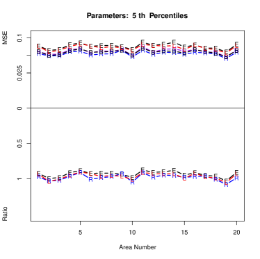
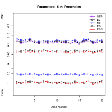
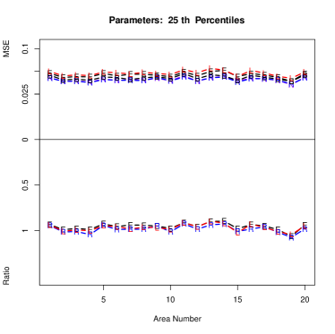
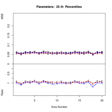
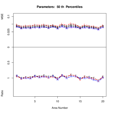
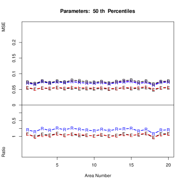
Figure 1: Area-specific MSEs (upper half of each plot) and ratios of bootstrap and simulated MSEs (lower half of each plot) for Scenarios (i) and (iv). In this setting, sample size $n=600$, number of bootstrap repetitions $B=100$, and $\mbox{$\boldsymbol{\betaup}$}=1.5\mbox{$\boldsymbol{\betaup}$}_{0}$.

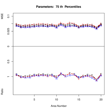
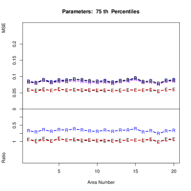
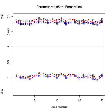
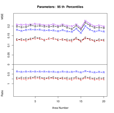
Figure 2: (continued) Area-specific MSEs (upper half of each plot) and ratios of bootstrap and simulated MSEs (lower half of each plot) for Scenarios (i) and (iv). In this setting, sample size $n=600$, number of bootstrap repetitions $B=100$, and $\mbox{$\boldsymbol{\betaup}$}=1.5\mbox{$\boldsymbol{\betaup}$}_{0}$.

The top portions of the plots in Figures 1 and 2 depict the area-specific MSEs of NER, EL, MR, EB, and EBEL. DIR and MQ are not included because their MSEs are much larger; including them masks the differences between the other methods. The lower portions of the plots give the ratios of the estimated and simulated AMSEs of EL, MR, and EBEL. The ratios of the other methods are not included because they do not perform well. The five plots in the left column are for Scenario (i), and these in the right column are for Scenario (iv). The results for Scenarios (ii) and (iii) are between those for (i) and (iv) and are not shown. The plots provide quick visual summaries of the performance.

There are six combinations of the sample sizes and signal-to-noise ratios. We have presented just one combination here. To save space, we include the results for the other five combinations in the supplementary file.

6.5 Illustration

Finite populations created based on statistical models are inevitably artificial. Ideally, we should judge new methods using real-world applications. This is not feasible, but we use a realistic example by downloading from the University of British Columbia library data centre the Survey of Labour and Income Dynamics (SLID) data provided by Statistics Canada (2014). According to the read-me file, this survey complements traditional survey data on labour market activity and income with an additional dimension: the changes experienced by individuals over time.

We are grateful to Statistics Canada for making the data set available, but we do not address the original goal of the survey here. Instead, we use it as a superpopulation to study the effectiveness of our small area quantile estimator.

After some data preprocessing, including removing units containing missing values, we retain 35488 sampling units and 6 variables. The variables are ttin, gender, age, yrx, tweek, and edu, i.e., total income, gender, age, years of experience, number of weeks employed, and education level. We transform ttin into $y=\log(2950+\mbox{ttin})$ so that its distribution is closer to symmetric, where $2950$ is the $5$th percentile of ttin. We ignore the sampling plan under which this data set was obtained. Instead, we examine how well our small area quantile predictors perform if we sample from this “real” population. We create 10 age groups:

$[0,\;20)$

$[20,\;25)$

$[25,\;30)$

$[30,\;35)$

$[35,\;40)$

$[40,\;45)$

$[45,\;50)$

$[50,\;55)$

$[55,\;60)$

$[60,\;\infty)$

Each age group is then divided into male and female subpopulations. This gives a finite population with 20 small domains (the small areas) based on age–gender combinations. The sizes of these small domains are as follows.

Male	1231	1525	1372	1337	1469	1536	1866	1890	1920	3089
Female	1200	1433	1449	1504	1497	1695	2053	2019	1944	3459

We first obtain the fitted values of the responses and residuals for all the units under the standard NER model. In each simulation repetition, we create a shadow population which keeps covariate $\mbox{\bf x}_{kj}$ unaltered but assembles new response value

$$y_{kj}=\hat{y}_{kj}+\hat{\epsilon}_{k,\pi(j)},$$

where $\pi(\cdot)$ is random permutation of $\{1,\ldots,n_{k}\}$. From this population, we sample $n_{k}=30$ units from area $k$ and estimate the 5%, 25%, 50%, 75%, and 95% small area quantiles using NER, EL, MR, and EBEL. For MR and EBEL, we assume that the values of $\mbox{\bf x}_{kj}$ are available for all units in the population. We omit the other methods because our simulation studies showed that they are less effective.

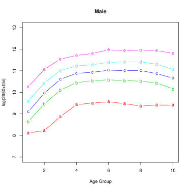
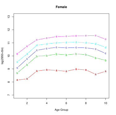
Figure 3: Small area population quantiles for SLID data. Lines a-d stand for area-specific 5%, 25%, 50%, 75% and 95% quantiles, respectively.

The population quantiles across the 10 age groups for both males and females are displayed in Figure 3. As expected, total income increases as age increases for all quantiles and both males and females. We see that compared with the 95% quantiles, the 5% quantiles for both males and females are much farther from the median. Hence, the small area population distributions of the response variable in all the small areas are skewed to the left. It is harder to obtain accurate estimates for the lower quantiles than for the upper quantiles.

We set the number of simulation repetitions to $500$. The simulated amse values and the ratio averages of the bootstrap and simulated MSEs are given in Table 3. The proposed EL and EBEL quantile estimators clearly have the best accuracy in terms of amse. Again, EL has surprisingly good performance, although it does not use census information. The performance of the bootstrap MSE estimates for EL and EBEL is satisfactory except for the 5% quantiles. This is likely due to the left skewness of the small area population distribution. The bootstrap MSE estimates work better for DIR than for MR.

7 Conclusions and discussions

We have proposed two general small area quantile estimation methods under a nested error linear model: the NER under a normal assumption on the error distribution and the EL under a DRM assumption on the error distribution. They are applicable whether or not census information on auxiliary variables is available. Simulation shows that when the error distribution is not normal, the DRM-based EL quantiles have superior performance. The proposed resampling amse estimates work reasonably well for quantiles in the middle range.

Supplementary material

The supplementary material contains proofs of Theorems 1–3 and some additional simulation results.

References

Anderson, J. A. (1979). Multivariate logistic compounds. Biometrika 66: 17–26.

Ballini, F., Betti, G., Carrette, S. and Neri, L. (2006). Poverty and inequality mapping in the Commonwealth of Dominica. Estudios Economicos 2: 123–162.

Battese, G. E., Harter, R. M. and Fuller, W. A. (1988). An error-components model for prediction of county crop areas using survey and satellite data. Journal of the American Statistical Association 80: 28–36.

Breckling, J. and Chambers, R. (1988). M-quantiles. Biometrika 75: 761–771.

Chambers, R. and Dunstan, R. (1986). Estimating distribution functions from survey data. Biometrika 73: 597–604.

Chambers, R. and Tzavidis, N. (2006). M–quantile models for small area estimation. Biometrika 93: 255–268.

Chaudhuri, S. and Ghosh, M. (2011). Empirical likelihood for small area estimation. Biometrika 98: 473–480.

Chambers, R., Chandra, H, Salvati, N and Tzavidis, N. (2011). Outlier robust small area estimation. Journal of Royal Statistical Society, B 76: 47–69.

Chen, J. and Liu, Y. (2013). Quantile and quantile-function estimations under density ratio model. The Annals of Statistics 4: 1669–1692.

Diallo, M. S. and Rao, J. N. K. (2016). Small area estimation of complex parameters under unit-level models with skew-normal errors. Manuscript.

Elbers, C. Lanjouw, J. O. and Lanjouw, P. (2003). Micro-level estimation of poverty and inequality. Econometrica 71: 355–364.

Estevao, V. M. and Sárndal, C. E. (2006). Survey estimates by calibration on complex auxiliary information. International Statistical Review 74: 127–147.

Fay, R. E. and Herriot, R. A. (1979). Estimates of income for small places: An application of James-Stein procedures to census data. Journal of the American Statistical Association 74: 269–277.

Ghosh, M., Maiti, T. and Roy, A. (2008). Influence functions and robust Bayes and empirical Bayes small area estimation. Biometrika 95: 573–585.

Guadarrama, M., Molina, I. and Rao, J. N. K. (2016). Small area estimation of general parameters under complex sampling designs. Manuscript.

Haslett, S. and Jones, G. (2005). Small area estimation using surveys and some practical and statistical issues. Statistics in Transition 7: 541–555.

Jiang, J. and Lahiri, P. S. (2006). Estimation of finite population domain means: A model-assisted empirical best prediction approach. Journal of the American Statistical Association 101: 301–311.

Jiang, J. and Nguyen, T. (2012). Small area estimation via heteroscedastic nested-error regression. The Canadian Journal of Statistics 40: 588–603.

Jiang, J., Nguyen, T. and Rao, J. S. (2010). Fence method for nonparametric small area estimation. Survey Methodology 36: 3–11.

Jiongo, V. D., Haziza, D. and Duchesne, P. (2013). Controlling the bias of robust small-area estimators. Biometrika 100: 843–858.

Keziou, A. and Leoni-Aubin, S. (2008). On empirical likelihood for semiparametric two-sample density ratio models. Journal of Statistical Planning and Inference 138: 915–928.

Koenker R. and Bassett, G. (1978). Regression quantiles. Econometrica 46: 33–50.

Kriegler, B. and Berk, R. (2010). Small area estimation of the homeless in Los Angeles: An application of cost-sensitive stochastic gradient boosting. The Annals of Applied Statistics 4: 1234–1255.

Lahiri, P. S. and Rao, J. N. K. (1995). Robust estimation of mean squared error of small area estimators. Journal of the American Statistical Association 90: 758–766.

Marchetti, S., Tzavidis, N. and Pratesi, M. (2012). Non-parametric bootstrap mean squared error estimation for M-quantile estimators of small area averages, quantiles and poverty indicators. Computational Statistics and Data Analysis 56: 2889–2902.

Molina, I. and Rao, J. N. K. (2010). Small area estimation of poverty indicators. The Canadian Journal of Statistics 38: 369–385.

Neri, L., Ballini F. and Betti, G. (2005). Poverty and inequality in transition countries. Statistics in Transition 7: 135–157.

Opsomer, J. D., Claeskens, G., Ranalli, M. G., Kauermann, G. and Breidt, F. J. (2008). Non-parametric small area estimation using penalized spline regression. Journal of the Royal Statistical Society: B 70: 265–286.

Owen, A. B. (1988). Empirical likelihood ratio confidence intervals for a single functional. Biometrika 75: 237–249.

Owen, A. B. (2001). Empirical Likelihood. New York: Chapman and Hall/CRC.

Pfeffermann, D. (2002). Small area estimation: New developments and directions. International Statistical Review 70: 125–143.

Pfeffermann, D. (2013). New important developments in small area estimation. Statistical Science 28: 40–68.

Pfeffermann, D. and Sverchkov, M. (2007). Small-area estimation under informative probability sampling of areas and within the selected areas. Journal of the American Statistical Association 102: 1427–1439.

Prasad, N. G. N. and Rao, J. N. K. (1990). The estimation of mean squared errors of small area estimators. Journal of the American Statistical Association 85: 163–171.

Qin, J. (1998). Inferences for case-control and semiparametric two-sample density ratio models. Biometrika 85: 619–630.

Qin, J. and Lawless, J. F. (1994). Empirical likelihood and general estimating equations. Annals of Statistics 22: 300–325.

Qin, J. and Zhang, B. (1997). A goodness-of-fit test for logistic regression models based on case-control data. Biometrika 84: 609–618.

Ranalli, M. G., Breidt, F. J. and Opsomer, J. D. (2016). Nonparametric regression methods for small area estimation. In Pratesi, M. (ed.), Analysis of Poverty Data by Small Area Estimation, New York: Wiley, pp. 187–204.

Rao, J. N. K. (2003). Small Area Estimation. New York: Wiley.

Rao, J. N. K. and Molina, I. (2015). Small Area Estimation. Hoboken, NY: Wiley.

Schaible, W. L. (1993). Use of small area estimators in U.S. federal programs. In Kalton, G., Kordos, J. and Platek, R. (eds), Small Area Statistics and Survey Designs, Warsaw: Central Statistical Office, I: 95–114.

Statistics Canada (2014). Survey of labour and income dynamics, 2011. Access: ABACUS. http://hdl.handle.net/10573/42961.

Tarozzi, A. and Deaton, A. (2009). Using census and survey data to estimate poverty and inequality for small areas. Review of Economics and Statistics 91: 773–792.

Tzavidis, N. and Chambers, R. (2005). Bias adjusted estimation for small areas with M-quantile models. Statistics in Transition 7: 707–713.

Tzavidis, N., Salvati, N., Pratesi, M. and Chambers, R. (2008). M-quantile models with application to poverty mapping. Statistical Methodology and Applications 17: 393–411.

Verret, F., Rao, J. N. K. and Hiridoglou, M. A. (2015). Model-based small area estimation under informative sampling. Survey Methodology 41: 333–347.

You, Y. and Rao, J. N. K. (2002). A pseudo-empirical best linear unbiased predictor approach to small area estimation using survey weights. Canadian Journal of Statistics 30: 431–439.

Zhang, B. (1997). Assessing goodness-of-fit of generalized logit models based on case-control data. Journal of Multivariate Analysis 82: 17–38.

Zhang, B. (2000). Quantile estimation under a two-sample semi-parametric model. Bernoulli 6: 491–511.

Table 1: amse  of small area quantile estimators under model (27)

Sample size $n=600$, number of repetitions 1000, $\mbox{$\boldsymbol{\betaup}$}=1.5\mbox{$\boldsymbol{\betaup}$}_{0}$

		AMSE
Scenario	$\alpha$	$5\%$	$25\%$	$50\%$	$75\%$	$95\%$
(i)	DIR	0.4242	0.1490	0.1244	0.1499	0.4324
	NER	0.0806	0.0659	0.0633	0.0656	0.0802
	EL	0.0878	0.0709	0.0682	0.0705	0.0875
	MQ	0.1926	0.0920	0.0764	0.0929	0.2021
	MR	0.0774	0.0657	0.0634	0.0650	0.0765
	EB	0.0797	0.0680	0.0660	0.0676	0.0789
	EBEL	0.0861	0.0729	0.0709	0.0724	0.0852
(ii)	DIR	0.3234	0.1404	0.1236	0.1405	0.3130
	NER	0.0753	0.0620	0.0569	0.0615	0.0741
	EL	0.0841	0.0695	0.0667	0.0690	0.0829
	MQ	0.1376	0.0819	0.0747	0.0823	0.1402
	MR	0.0708	0.0603	0.0571	0.0600	0.0704
	EB	0.0729	0.0629	0.0590	0.0628	0.0722
	EBEL	0.0805	0.0711	0.0691	0.0709	0.0799
(iii)	DIR	0.7323	0.1634	0.0977	0.1025	0.2597
	NER	0.2034	0.0821	0.0712	0.0576	0.1118
	EL	0.1303	0.0573	0.0521	0.0540	0.0681
	MQ	0.4028	0.1162	0.0567	0.0641	0.1607
	MR	0.1756	0.0852	0.0699	0.0560	0.1206
	EB	0.1950	0.0848	0.0737	0.0594	0.1146
	EBEL	0.1284	0.0572	0.0539	0.0549	0.0633
(iv)	DIR	0.2621	0.1028	0.0975	0.1627	0.7385
	NER	0.1138	0.0589	0.0720	0.0835	0.2060
	EL	0.0684	0.0551	0.0529	0.0584	0.1313
	MQ	0.0983	0.0518	0.0534	0.1020	0.4117
	MR	0.1228	0.0572	0.0708	0.0870	0.1774
	EB	0.1169	0.0606	0.0746	0.0866	0.1970
	EBEL	0.0636	0.0560	0.0549	0.0586	0.1291

Table 2: Average ratios of estimated and simulated MSEs under model (27)

Sample size $n=600$, $B=100$, $\mbox{$\boldsymbol{\betaup}$}=1.5\mbox{$\boldsymbol{\betaup}$}_{0}$, number of repetitions 1000

Scenario	$\alpha$	$5\%$	$25\%$	$50\%$	$75\%$	$95\%$
(i)	DIR	0.9693	0.9835	0.9892	0.9780	0.9535
	EL	0.9307	0.9536	0.9607	0.9546	0.9322
	MR	0.9784	0.9823	0.9901	0.9904	0.9906
	EBEL	0.9574	0.9686	0.9732	0.9716	0.9686
(ii)	DIR	0.9819	0.9663	0.9683	0.9774	0.9939
	EL	0.8830	0.9150	0.9411	0.9296	0.9016
	MR	0.9525	0.9503	0.9769	0.9586	0.9637
	EBEL	0.9143	0.9310	0.9503	0.9381	0.9243
(iii)	DIR	0.9564	0.9463	0.9915	0.9977	0.9845
	EL	0.7006	0.9769	0.9787	0.9739	0.9585
	MR	0.3874	0.6753	0.8014	1.0265	0.5598
	EBEL	0.7430	0.9830	0.9817	0.9800	0.9757
(iv)	DIR	0.9723	0.9938	0.9918	0.9505	0.9541
	EL	0.9549	0.9466	0.9523	0.9568	0.6942
	MR	0.5508	1.0016	0.7882	0.6631	0.3841
	EBEL	0.9733	0.9563	0.9564	0.9538	0.7399

Table 3: Simulation results of small area quantile estimators based on SLID data

Sample size $n=600$, $B=100$ for bootstrap, number of repetitions $500$.

	AMSE
$\alpha$	$5\%$	$25\%$	$50\%$	$75\%$	$95\%$
DIR	0.1903	0.0455	0.0208	0.0201	0.0882
NER	0.0709	0.0259	0.0205	0.0165	0.0419
EL	0.0712	0.0153	0.0136	0.0141	0.0205
MQ	0.1144	0.0347	0.0141	0.0259	0.1011
MR	0.0573	0.0258	0.0197	0.0157	0.0438
EB	0.0689	0.0246	0.0188	0.0160	0.0430
EBEL	0.0712	0.0150	0.0131	0.0140	0.0212
	Ratio of bootstrapped and simulated MSEs
$\alpha$	$5\%$	$25\%$	$50\%$	$75\%$	$95\%$
DIR	1.1722	0.8961	1.1356	1.1552	1.1412
EL	0.4501	0.9066	0.9202	0.9966	0.8805
MR	0.4063	0.5612	0.6694	1.0420	0.4576
EBEL	0.3462	0.8469	0.9143	0.9544	0.8115