Periapsis shift and deflection of light by hairy black holes

Abstract

We investigate the orbit equations and the eikonal equation for light respectively, under influence of the hairy black holes (asymptotically flat) in fourth dimensions. We consider two hairy black hole solutions with non-trivial potentials, and one of these solutions has Schwarzschild case as a smooth limit. Following to Landau and Lifshitz we use the Hamilton-Jacobi method, and we show hairy corrections for periapsis shift, where the effect of the hair is to increase it. In the same way, using the eikonal equation we show the deflection of the light and the relevant scalar hair corrections. Interestingly we find that the hair screening the gravitational field, decreasing the angle of deflection as the hair increases.

1 Introduction

The Hamilton-Jacobi formalism was applied in different gravity situations, for example in the context of AdS/CFT Maldacena:1997re it was used to find counterterms Martelli:2002sp ; Batrachenko:2004fd . On the other hand, the Hamilton-Jacobi equations of canonical gravity are the main tool in the derivation of renormalization group equations deBoer:2000cz ; Heemskerk:2010hk .

The scalar field has a fundamental structure in string theory, and the expectation value controls the string coupling constant $g_{s}=\langle e^{\phi}\rangle$. In high energy physics the scalar field is the Higgs particle Aad:2012tfa , and in Cosmology is the $inflaton$ that describes cosmological perturbations observed in the experiments COBE, WMAP and Planck Spergel:2006hy ; Planck:2013jfk . In the context of AdS/CFT the scalar field is a source of the boundary operators. Interestingly the hairy solutions studied here can be obtained from his asymptotically AdS solution. By suitably adjusting the cosmological constant or the scalar field potential so that the effective cosmological vanishes, one can obtain asymptotically flat black holes Anabalon:2013qua . We considered the boundary condition of a scalar field such that $\phi=0$ (at spatial infinity). In Anabalon:2013qua ; Anabalon:2012ih ; Gibbons:1987ps was constructed various exact and regular solutions of hairy black holes (charged) asymptotically flat, and AdS Anabalon:2012ta ; Anabalon:2012ih ; Anabalon:2012dw . Is important understanding that the hair (scalar field) lives behind horizon and boundary, and does not exist a conserved quantity associated with the scalar field. In Anabalon:2013qua ; Nunez:1996xv argument that the back-reaction ensure that the scalar field can over in a strong gravitational field without collapsing completely. In the present paper, we considered Einstein-dilaton theories minimally coupled and with non-trivial potentials, in Nunez:1996xv ; Anabalon:2012ih ; Anabalon:2012dw constructed hairy black holes in dilaton-charged gravity theories without scalar potential, in these cases the coupling of the dilaton with gauge fields ensures the existence of an effective potential. In the extremal case the near horizon data depend completely by the electric and magnetic charges and so the attractor mechanism Ferrara:1995ih ; Strominger:1996kf ; Ferrara:1996dd works like the no-hair theorem.

To describe the geodesics (and null geodesic) we need to consider two actions, one for the gravitational field which describes the geometric of space-time for a given distribution of matter $T_{\mu\nu}$. The another action gives us information about how the particles (of mass $m$) moves in that space-time and is given by

$$I=-mc\int_{a}^{b}ds$$ (1)

where $ds$ is the infinitesimal line universe $ds^{2}=g_{\mu\nu}dx^{\mu}dx^{\nu}$. Taking the variation we get the geodesic equation

$$\frac{d^{2}x^{\mu}}{ds^{2}}+\Gamma_{\alpha\beta}^{\mu}\frac{dx^{\alpha}}{ds}\frac{dx^{\beta}}{ds}=0$$ (2)

but to describe the null geodesics ($ds=0$) the before equation is not complete. The Hamilton-Jacobi is a powerful method to obtain the orbit equations. Landau-Lifshitz showed that the Hamilton-Jacobi equation for a particle in any space-time is $(\mathcal{M},g)$

$$g^{\mu\nu}\frac{\partial I}{\partial x^{\mu}}\frac{\partial I}{\partial x^{\mu}}-m^{2}=0$$ (3)

In literature there is an extensive bibliography about the study of the orbits of several black holes in different theories Frye:2013xia ; Cruz:2004ts ; Magnan:2007uw ; Cruz:2011yr ; Wells:2011st ; Hackmann:2008zz ; Olivares:2013zta . Recently was study Light propagation in a plasma on Kerr space-time using the Hamilton-Jacobi equation Perlick:2017fio , but in fourth dimensions is complicated find a rotated hairy black holes, although there are currently several solutions in three dimensions Correa:2012rc ; Natsuume:1999at .

For light trajectory (null geodesic) we consider the null module condition for four-vector wave $k_{\mu}k^{\mu}=0$. So, replacing $k_{\mu}=\partial\psi/\partial x^{\mu}$ we find eikonal equation in a gravitational field

$$g^{\mu\nu}\frac{\partial\psi}{\partial x^{\mu}}\frac{\partial\psi}{\partial x^{\mu}}=0$$ (4)

The present paper is structured as follows: In section 2, we consider a small review of Newtonian results and its corrections given by general relativity. In section 3, we present the two hairy solutions and its properties, in the section 4 we use the holographic stress tensor method to determine the mass of hairy black holes. Finally, in section 5, following to intuitive procedure of section 2, we calculate the periapsis shift and deflection of light for both hairy black holes, and in the final part, we present the conclusions.

2 Hamilton-Jacobi method in Schwarzschild

The Kepler problem in celestial mechanics consist in found and solve the orbit equations of stellar systems (two body system). Classically is solved (exactly) considering the Newtonian potential

$$U_{N}(r)=-\frac{G_{N}mm^{{}^{\prime}}}{r}$$ (5)

And we can be solved alternatively by Hamilton-Jacobi method. Considering the Lagrangian expression for a particle in the central field force (at the plane $\theta=\pi/2$)

$$L=\frac{m}{2}(\dot{r}^{2}+r^{2}\dot{\varphi}^{2})-U_{N}(r),\qquad M=\frac{\partial L}{\partial\dot{\varphi}}=mr^{2}\dot{\varphi}$$ (6)

The Hamilton-Jacobi equation is

$$\frac{1}{2m}\biggl{(}\frac{\partial I}{\partial r}\biggr{)}^{2}+\frac{1}{2mr^{2}}\biggl{(}\frac{\partial I}{\partial\varphi}\biggr{)}^{2}+U_{N}(r)=\mathcal{E}^{{}^{\prime}}$$ (7)

where the ansatz is $I(r)=-\mathcal{E}^{{}^{\prime}}t+M\varphi+I_{r}^{(0)}$ and its solution is

$$I(r)=-\mathcal{E}^{{}^{\prime}}t+M\varphi+\int{\sqrt{2m(\mathcal{E}^{{}^{\prime}}-U_{N})-\frac{M^{2}}{r^{2}}}dr}$$ (8)

The trajectory is given by equation $\frac{\partial I}{\partial M}=cte$

$$\varphi(r)=\int\frac{Mdr}{r^{2}\sqrt{2m(\mathcal{E}^{{}^{\prime}}-U_{N})-\frac{M^{2}}{r^{2}}}}+\varphi_{0}\Rightarrow\frac{p}{r}=1+e\cos{(\varphi-\varphi_{0})}$$ (9)

Where $p=M^{2}/m^{2}m^{{}^{\prime}}G_{N}$ and the eccentricity is $e=\sqrt{1+2\mathcal{E}^{{}^{\prime}}p/G_{N}mm^{{}^{\prime}}}$. Is easy to show that for elliptical orbit $e<1$

$$\Delta\varphi^{(0)}=-\frac{\partial\Delta I_{r}^{(0)}}{\partial M}=2\int_{r_{min}}^{r_{max}}\frac{Mdr}{r^{2}\sqrt{2m(\mathcal{E}^{{}^{\prime}}-U_{N})-\frac{M^{2}}{r^{2}}}}=2\pi$$ (10)

This is the angle that vector position tour when $r$ changed from $r_{max}$ to $r_{min}$ and return to $r_{max}$. The astronomical observations showed that perihelion of Mercury has deviations $\Delta\varphi^{(0)}\rightarrow\Delta\varphi^{(0)}+\delta\varphi$ . Exist different forms to deal with this problem, classically we can consider perturbations to Newtonian potential $U_{N}\rightarrow U_{N}+\delta U(r)$ Landau ; LandauL ; Wells:2011st . Another option is to consider the corrections of general relativity. The usual method consist in to solve the geodesic equation Magnan:2007uw , but here we focus on the Hamilton-Jacobi method Vasudevan:2005js .

2.1 General relativistic corrections

In this section, we describe step by step the procedure proposed by Landau and Lifshitz Landau . This gives us a correct intuition when we face the hairy case. We will consider the very know Schwarzschild asymptotically flat solution, where the action is

$$S[g_{\mu\nu}]=\frac{1}{2\kappa}\int_{\mathcal{M}}{d^{4}x\sqrt{-g}R}+\frac{1}{\kappa}\int_{\partial\mathcal{M}}{d^{3}xK\sqrt{-h}}$$ (11)

Here $\kappa=8\pi G_{N}$, and the last term is the Gibbons-Hawking boundary term. Where $h_{ab}$ is the boundary metric and $K$ is the trace of the extrinsic curvature. The solution is

$$ds^{2}=-c^{2}N(r)dt^{2}+\frac{dr^{2}}{N(r)}+r^{2}(d\theta^{2}+\sin^{2}{\theta}d\varphi^{2})$$ (12)

where, $N(r)=1-r_{g}/r$ and $r_{g}=2G_{N}m^{{}^{\prime}}/c^{2}$. Here $m^{{}^{\prime}}$ is the gravitational mass. Considering geodesics in the plane $\theta=\pi/2$. The Hamilton-Jacobi equation of the trajectory is

$$\frac{1}{c^{2}N(r)}\biggl{(}\frac{\partial I}{\partial t}\biggr{)}^{2}-N(r)\biggl{(}\frac{\partial I}{\partial r}\biggr{)}^{2}-\frac{1}{r^{2}}\biggl{(}\frac{\partial I}{\partial\varphi}\biggr{)}^{2}-m^{2}c^{2}=0$$ (13)

The ansatz is $I(t,r,\varphi)=-\mathcal{E}_{0}t+M\varphi+I_{r}(r)$, where the energy and mass of particle is $\mathcal{E}_{0}$, $m$, and its angular momentum is $M$. Replacing the expression $I(t,r,\varphi)$ in (13) we can solve $I_{r}$

$$I_{r}(r)=\int{\biggl{[}\frac{r^{2}(\mathcal{E}_{0}^{2}-m^{2}c^{4})+m^{2}c^{4}rr_{g}}{c^{2}(r-r_{g})^{2}}-\frac{M^{2}}{r(r-r_{g})}\biggr{]}}^{1/2}dr$$ (14)

The trajectory equation can be determined by $\varphi(r)=-\frac{\partial I_{r}}{\partial M}+cte$, and is easy to show

$$\varphi(r)=\int\biggl{[}r^{2}\sqrt{\frac{\mathcal{E}_{0}^{2}}{c^{2}}-\biggl{(}m^{2}c^{2}+\frac{M^{2}}{r^{2}}\biggr{)}\biggl{(}1-\frac{r_{g}}{r}\biggr{)}}\biggr{]}^{-1}Mdr+cte$$ (15)

The classical limit given in (9) can be obtained considering $c\rightarrow\infty$, $r_{g}=0$ and $\mathcal{E}_{0}=mc^{2}+\mathcal{E}^{{}^{\prime}}$. Here $\mathcal{E}^{{}^{\prime}}$ is the non-relativistic energy. To obtain the relevant corrections of general relativity we consider small velocities of the planets respect to light, this means $r_{g}/r<<1$. The angular change of closed orbits can be calculated in the similar form to (10)

$$\Delta\varphi(r)=-\frac{\partial\Delta I_{r}}{\partial M}$$ (16)

For that purpose, we need expand (14) and check the Newtonian term and its relativistic correction. Comparing $M^{2}/r^{2}$ part of (8) and (14) is easy concluded that we need to consider the change variable

$$r(r-r_{g})=r^{{}^{\prime}2}\Rightarrow r-\frac{r_{g}}{2}\approx r^{{}^{\prime}}$$ (17)

and introducing the non-relativistic energy $\mathcal{E}^{{}^{\prime}}$. Expanding around $r_{g}/r<<1$ keeping fix $M^{2}/r^{2}$ (regardless of the apostrophe) we have

$$I_{r}=\int\sqrt{2m(E-U)-\frac{M^{2}}{r^{2}}+\frac{3m^{2}c^{2}r_{g}^{2}}{2r^{2}}+O\biggl{(}\frac{r_{g}^{3}}{r^{3}}\biggr{)}}dr$$ (18)

where

$$E=\mathcal{E}^{{}^{\prime}}+\frac{\mathcal{E}^{{}^{\prime}2}}{c^{2}},\qquad U=U_{N}\biggl{(}1+\frac{4\mathcal{E}^{{}^{\prime}}}{mc^{2}}\biggr{)},\qquad U_{N}=-\frac{mm^{{}^{\prime}}G_{N}}{r}$$ (19)

We can see the fundamental correction to $M^{2}/r^{2}$ is given by the term $r_{g}^{2}/r^{2}$, and this term can describe the periapsis shift of the orbit. We consider $E\approx\mathcal{E}^{{}^{\prime}}$, $U\approx U_{N}$ and only expanding around $r_{g}/r<<1$ keeping fix $M^{2}/r^{2}$

$$I_{r}\approx\int\sqrt{2m(\mathcal{E}^{{}^{\prime}}-U_{N})-\frac{M^{2}}{r^{2}}}~{}dr+\frac{3m^{2}c^{2}r_{g}^{2}}{4}\int\frac{1}{r^{2}}\biggl{[}\sqrt{2m(\mathcal{E}^{{}^{\prime}}-U_{N})-\frac{M^{2}}{r^{2}}}\biggr{]}^{-1}dr+\ldots$$ (20)

Considering the limits of integration $(r_{min},r_{max})$, we have $I_{r}\rightarrow\Delta I_{r}$

$$\Delta I^{(0)}_{r}=\int_{r_{min}}^{r_{max}}\sqrt{2m(\mathcal{E}^{{}^{\prime}}-U_{N})-\frac{M^{2}}{r^{2}}}~{}dr$$ (21)

So 

$$\Delta I_{r}\approx\Delta I_{r}^{(0)}-\frac{3m^{2}c^{2}r_{g}^{2}}{4M}~{}\frac{\partial\Delta I_{r}^{(0)}}{\partial M}$$ (22)

then, using (16) is easy to show the correction given for general relativity

$$\Delta\varphi\approx 2\pi+\frac{6\pi G_{N}^{2}m^{2}m^{{}^{\prime}2}}{c^{2}M^{2}}$$ (23)

To determine the trajectory of light ray (null geodesics) we need the eikonal equation (4). This equation is similar to (13) with $m^{2}=0$ and $I\rightarrow\psi$, and in this case, instead of energy $\mathcal{E}=-\partial I/\partial t$ of the particle, we consider the light frequency $\omega_{0}=-\partial\psi/\partial t$, then

$$\psi(r)=-\omega_{0}t+M\varphi+\psi_{r}(r)$$ (24)

From eikonal equation we have

$$\psi_{r}(r)=\frac{\omega_{0}}{c}\int\biggl{[}\frac{r^{2}}{(r-r_{g})^{2}}-\frac{\varrho^{2}}{r(r-r_{g})}\biggr{]}^{1/2}dr,\qquad\varrho=\frac{Mc}{\omega_{0}}$$ (25)

where $\varrho$ is the impact parameter. One more time we need consider the before transformations given in (17)

$$\psi_{r}(r)\approx\frac{\omega_{0}}{c}\int\biggl{(}1+\frac{2r_{g}}{r}-\frac{\varrho^{2}}{r^{2}}\biggr{)}^{1/2}dr$$ (26)

the equation for the trajectory of a light ray is $\varphi(r)=-\frac{\partial\psi_{r}}{\partial M}+cte$, then

$$\varphi(r)=\int\frac{1}{r^{2}}\biggl{[}\sqrt{\frac{1}{\varrho^{2}}-\frac{1}{r^{2}}\biggl{(}1-\frac{r_{g}}{r}\biggr{)}}\biggr{]}^{-1}dr+cte$$ (27)

the gravitational correction is given by $r_{g}$, if we take $r_{g}=0$ the integral is $r=\varrho/\cos{\varphi}$. Namely a line that passing a distance $\varrho$ from the origin, integrating (26) when $r_{g}=0$

$$\Delta\psi_{r}^{(0)}=\frac{\omega_{0}}{c}\int_{0}^{\pi}\sqrt{1-\frac{\varrho^{2}}{r^{2}}}dr=-M\pi$$ (28)

The angle formed by the asymptotes of ray light that comes from a very great distance $(r\rightarrow\infty,\varphi=-\pi/2)$, approaches the nearest point $(r=\varrho,\varphi=0)$ and moves away a great distance $(r\rightarrow\infty,\varphi=\pi/2)$, is $\Delta\varphi^{(0)}=-\partial\Delta\psi_{r}^{(0)}/\partial M=\pi$. The relativistic corrections are given by

$$\Delta\varphi=-\frac{\partial\Delta\psi_{r}}{\partial M}$$ (29)

and for that purpose we need expand (26) around $r_{g}/r<<1$ (keeping constant $\varrho^{2}/r^{2}$)

$$\psi_{r}(r)\approx\psi^{(0)}_{r}+\frac{r_{g}\omega_{0}}{c}\ln{\varrho}+\frac{r_{g}\omega_{0}}{c}\cosh^{-1}\biggl{(}\frac{r}{\varrho}\biggr{)}$$ (30)

The term $\psi^{(0)}_{r}$ corresponds to the classical ray rectilinear $\psi_{r}(r_{g}=0)=\psi^{(0)}_{r}$ in (26). The total changing of $\psi_{r}$ during propagation of the light, from one large distance $R$ at the point $r=\varrho$ close to the center and back again to the distance $R$ is

$$\Delta\psi_{r}=\Delta\psi^{(0)}_{r}+\frac{2r_{g}\omega_{0}}{c}\cosh^{-1}\biggl{(}\frac{r}{\varrho}\biggr{)}$$ (31)

replacing in (29)

$$\Delta\varphi=-\frac{\partial\Delta\psi^{(0)}_{r}}{\partial M}+\frac{2r_{r}R}{\varrho\sqrt{R^{2}-\varrho^{2}}}=\Delta\varphi^{(0)}+\frac{2r_{r}R}{\varrho\sqrt{R^{2}-\varrho^{2}}}$$ (32)

taking the limit $R\rightarrow\infty$ and remember that $\Delta\varphi^{(0)}=\pi$ for the rectilinear ray, we obtain

$$\Delta\varphi=\pi+\frac{2r_{g}}{\varrho}$$ (33)

3 Hairy black hole solutions

We will consider two hairy solutions one of which is the smooth limit of the first when the hairy parameter $\nu\rightarrow\infty$. We are interested in asymptotically flat hairy black hole solutions with a spherical horizon Anabalon:2013sra ; Anabalon:2013eaa . The action is

$$S[g_{\mu\nu},\phi]=\frac{1}{2\kappa}\int_{\mathcal{M}}{d^{4}x\sqrt{-g}\biggl{[}R-\frac{(\partial\phi)^{2}}{2}-V(\phi)\biggr{]}}+\frac{1}{\kappa}\int_{\partial\mathcal{M}}{d^{3}xK\sqrt{-h}}+S^{ct}$$ (34)

where $V(\phi)$ is the scalar potential, $\kappa=8\pi G_{N}$ and $S^{ct}$ is the boundary counterterm which we use for constructed the renormalized quasi-local stress tensor $\tau_{ab}$. The equations of motion for the dilaton and metric are

$$\frac{1}{\sqrt{-g}}\partial_{\mu}\left(\sqrt{-g}g^{\mu\nu}\partial_{\nu}\phi\right)-\frac{\partial V}{\partial\phi}=0$$

$$E_{\mu\nu}=R_{\mu\nu}-\frac{1}{2}g_{\mu\nu}R-\frac{1}{2}T_{\mu\nu}^{\phi}$$

where the stress tensor of the scalar field is

$$T_{\mu\nu}^{\phi}=\partial_{\mu}\phi\partial_{\nu}\phi-g_{\mu\nu}\left[\frac{1}{2}\left(\partial\phi\right)^{2}+V(\phi)\right]$$

When we consider convex or positive semi-definite potential the no-hair theorems ensure that does not exist regular black holes solutions Israel:1967wq ; Bekenstein:1995un ; Sudarsky:1995zg . In Martinez:2006an ; Acena:2013jya ; Anabalon:2013sra ; Anabalon:2013qua ; Acena:2012mr ; Anabalon:2012dw they were able to relax some of those conditions and find a large (exact) family of hairy black holes. In the present article, we will work with following potentials, where $l_{\nu}^{-1}=\sqrt{(\nu^{2}-1)/2\kappa}$ and $j^{-1}=1/\sqrt{2\kappa}$

$$V(\phi) =\frac{2\alpha}{\nu^{2}}\biggl{[}\frac{\nu-1}{\nu+2}\sinh{\phi l_{\nu}(\nu+1)}-\frac{\nu+1}{\nu-2}\sinh{\phi l_{\nu}(\nu-1)}+4\frac{\nu^{2}-1}{\nu^{2}-4}\sinh{\phi l_{\nu}}\biggr{]}$$ (35)

$$V(\phi)=\frac{\alpha j\phi}{\kappa}[2+\cosh(j\phi)]-\frac{3\alpha}{\kappa}\sinh(j\phi)$$ (36)

Along the present paper, we centered in the negative branch: $\phi\in(-\infty,0]$ for which $\alpha>0$

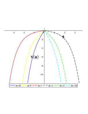
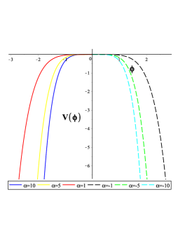
Figure 1: The left hand side graphic (a) describe the potential (35) at $\nu=5$. There are two families: $\phi\in(-\infty,0]$ for which $\alpha>0$ and $\phi\in[0,+\infty)$ for which $\alpha<0$.
The right hand side graphic (b) describe the potential (36). There are two families: $\phi\in(-\infty,0]$ for which $\alpha>0$ and $\phi\in[0,+\infty)$ for which $\alpha<0$.

3.1 Black hole solution

Considering the action (34) with scalar potential (35) and the metric ansatz

$$ds^{2}=\Omega(x)\left[-c^{2}f(x)dt^{2}+\frac{\eta^{2}dx^{2}}{f(x)}+d\theta^{2}+\sin^{2}\theta d\phi^{2}\right]$$ (37)

The equations of motion can be integrated for the conformal factor Anabalon:2013sra ; Anabalon:2013qua ; Acena:2012mr ; Acena:2013jya :

$$\Omega(x)=\frac{\nu^{2}x^{\nu-1}}{\eta^{2}(x^{\nu}-1)^{2}}$$ (38)

where the parameters that characterize the hairy solutions are $\alpha$ and $\nu$. The solutions for scalar field

$$\phi(x)=l_{\nu}^{-1}\ln{x}$$ (39)

and metric function

$$f(x)=\alpha\biggl{[}\frac{1}{\nu^{2}-4}-\frac{x^{2}}{\nu^{2}}\biggl{(}1+\frac{x^{-\nu}}{\nu-2}-\frac{x^{\nu}}{\nu+2}\biggr{)}\biggr{]}+\frac{x}{\Omega(x)}$$ (40)

where $\eta$ is the only integration constant and $l_{\nu}^{-1}=\sqrt{(\nu^{2}-1)/2\kappa}$.

The scalar potential given in (35) and the solution for $\Omega(x),\phi(x),f(x)$ are invariant under the transformation $\nu\rightarrow-\nu$. The boundary where $\Omega(x)$ is blowing-up correspond to $x=1$ and the theory has a standard flat vacuum $V(\phi=0)=0$. The hairy parameter vary in the range $\nu\in[1,+\infty)$, and in the limit $\nu=1$ one gets $l_{\nu}\rightarrow\infty$ and $\phi\rightarrow 0$ so that the Schwarzschild black hole (asymptotically flat) is smoothly obtained.
There are two distinct branches, one that corresponds to $x\in(0,1]$ and the other one to $x\in[1,\infty)$ — the curvature singularities are at $x=0$ for the first branch and $x\rightarrow\infty$ for the second one (these are the locations where the scalar field is also blowing up). Considering the change of coordinates

$$x=1-\frac{1}{\eta r}+\frac{(\nu^{2}-1)}{24\eta^{3}r^{3}}\biggl{[}1+\frac{1}{\eta r}-\frac{9(\nu^{2}-9)}{80\eta^{2}r^{2}}\biggr{]}+O(r^{-6})$$ (41)

we can read off the mass from the sub-leading term of $g_{tt}$:

$$-g_{tt}=f(x)\Omega(x)=1-\frac{\alpha+3\eta^{2}}{3\eta^{3}r}+O(r^{-3})$$ (42)

In the section (4) we use the quasilocal stress tensor to show that the mass of this black hole is

$$m_{1}^{{}^{\prime}}=\frac{4\pi c^{2}}{\kappa}\biggl{(}\frac{\alpha+3\eta^{2}}{3\eta^{3}}\biggr{)}$$ (43)

where the gravitational radio (or mass parameter) is $r_{g}=2m_{1}^{{}^{\prime}}G_{N}/c^{2}$ In the section (4) we verified that this is the gravitational mass of the black hole

3.2 Black hole solution $\nu=\infty$

In Anabalon:2013qua , was studied the following solution, but here we consider the neutral case.
One more time, considering the action (34) with scalar potential (36) and the metric ansatz

$$ds^{2}=\Omega(x)\left[-c^{2}f(x)dt^{2}+\frac{\eta^{2}dx^{2}}{x^{2}f(x)}+d\theta^{2}+\sin^{2}{\theta}d\phi^{2}\right]$$ (44)

The equations of motion can be integrated for the conformal factor Anabalon:2013sra ; Anabalon:2013qua :

$$\Omega(x)=\frac{x}{\eta^{2}\left(x-1\right)^{2}}$$ (45)

Where $\alpha$ is the parameter that characterizes the hairy solution. With this choice of the conformal factor is straightforward to obtain the expressions for the scalar field

$$\phi(x)=j^{-1}\ln{x},\qquad j^{-1}=\frac{1}{\sqrt{2\kappa}}$$ (46)

and the metric function

$$f(x)=\alpha\left[\frac{(x^{2}-1)}{2x}-\ln(x)\right]+\frac{1}{\Omega(x)}$$ (47)

At the boundary $\Omega(x)$ is blowing-up, this correspond to $x=1$. The theory has a standard flat vacuum $V(\phi=0)=0$. There are two distinct branches, one that corresponds to $x\in(0,1]$ and the other one to $x\in[1,\infty)$ — the curvature singularities are at $x=0$ for the first branch and $x\rightarrow\infty$ for the second one (these are the locations where the scalar field is also blowing up). But the difference with the before hairy solution is that does not exist a hairy parameter, and we can not obtain the Schwarzschild case.
Here, $\eta$ is the constant of integration and considering the horizon equation we can solve it

$$f(\eta,x_{h})=0\rightarrow\eta^{2}=\frac{x_{h}}{(x_{h}-1)^{2}}\biggl{[}\frac{\alpha(2x_{h}\ln{x_{h}}-x_{h}^{2}+1)}{2x_{h}}\biggr{]}$$ (48)

Considering the following asymptotic coordinate transformation

$$x=1-\frac{1}{\eta r}+\frac{1}{2\eta^{2}r^{2}}-\frac{1}{8\eta^{3}r^{3}}+O(r^{-5})$$ (49)

the gravitational radio $r_{g}$ (or mass parameter) can be read-off $-g_{tt}$ component in r-coordinate

$$\Omega(x)f(x)=1-\frac{\alpha}{6\eta^{3}r}+O(r^{-3})$$ (50)

then $r_{g}=\alpha/6\eta^{3}$, and the mass of the hairy black hole is

$$m_{2}^{{}^{\prime}}=\frac{4\pi c^{2}}{\kappa}r_{g}=\frac{c^{2}}{2G_{N}}\biggl{(}\frac{\alpha}{6\eta^{3}}\biggr{)},\qquad$$ (51)

In the next section (4) we verified that this is the gravitational mass of the black hole

4 Mass of hairy black holes

Similar to holographic formalism for asymptotic AdS space-times Myers:1999psa ; Anabalon:2015ija ; Anabalon:2015xvl ; Anabalon:2016izw ; Balasubramanian:1999re , for asymptotically-flat exist an identical proposal given in Astefanesei:2005ad ; Astefanesei:2009wi ; Astefanesei:2006zd ; Astefanesei:2010bm . If the boundary has the following topology $S^{2}\times R\times S^{1}$ the gravitational counterterm is

$$S^{ct}=-\frac{1}{\kappa}\int_{\partial\mathcal{M}}d^{3}x\sqrt{2\mathcal{R}}~{}\sqrt{-h}$$ (52)

The (quasilocal) stress tensor was defined in Brown:1992br like

$$\tau_{ab}\equiv\frac{2}{\sqrt{-h}}\frac{\delta S}{\delta h^{ab}}$$ (53)

where for the total action (that including the boundary terms) given in (34) we have Astefanesei:2005ad

$$\tau_{ab}=-\frac{1}{\kappa}\left[K_{ab}-h_{ab}K-\Psi(\mathcal{R}_{ab}-\mathcal{R}h_{ab})-h_{ab}\Box\Psi+\Psi_{;ab}\right]$$ (54)

Considering the foliation ($x=constant$) of the metrics (37) and (44) (both foliations are similar)

$$h_{ab}dx^{a}dx^{b}=\Omega(x)[-c^{2}f(x)dt^{2}+d\theta^{2}+\sin^{2}{\theta}d\varphi^{2}]$$ (55)

Where $\mathcal{R}_{ab}$, $\mathcal{R}$ are the Ricci tensor and Ricci scalar of the foliation (55). The expression for $\Psi$ was given in Astefanesei:2006zd , this is $\Psi=\sqrt{2/\mathcal{R}}$, then

$$\mathcal{R}_{00}=0\quad,\quad\mathcal{R}_{\theta\theta}=1\quad,\quad\mathcal{R}_{\varphi\varphi}=\sin^{2}\theta\quad,\quad\mathcal{R}=\frac{2}{\Omega(x)}\quad,\quad\Psi=\sqrt{\Omega(x)}$$ (56)

Here $K_{ab}$, $K$ and $n_{a}$ are the extrinsic curvature, its trace and the normal of time-like hypersurface defined by induced metric (55). We use the following very useful expressions

$$K_{ab}=\frac{\sqrt{g^{xx}}}{2}\partial_{x}h_{ab},\qquad n_{a}=\frac{\delta_{a}^{x}}{\sqrt{g^{xx}}},\qquad K\sqrt{-h}=n^{a}\partial_{a}\sqrt{-h}$$ (57)

And is easy to show $T^{\nu}_{tt}$ for solution (37) and $T^{\infty}_{tt}$ for (44)

$$T^{\nu}_{tt}=-\frac{c^{2}}{\kappa}\biggl{[}-\frac{(\Omega f)^{{}^{\prime}}}{2\eta}\sqrt{\frac{f}{\Omega}}+\frac{\sqrt{\Omega f}}{2\eta}\biggl{(}\frac{3\Omega^{{}^{\prime}}f}{\Omega}+f^{{}^{\prime}}\biggr{)}-2\sqrt{\Omega}f\biggr{]}$$ (58)

$$T^{\infty}_{tt}=-\frac{c^{2}}{\kappa}\biggl{[}-\frac{x(\Omega f)^{{}^{\prime}}}{2\eta}\sqrt{\frac{f}{\Omega}}+\frac{x\sqrt{\Omega f}}{2\eta}\biggl{(}\frac{3\Omega^{{}^{\prime}}f}{\Omega}+f^{{}^{\prime}}\biggr{)}-2\sqrt{\Omega}f\biggr{]}$$ (59)

The conserved quantity associated with the generator of time translations symmetry $\xi=\partial/c\partial t$ is the energy. For both metrics (37) and (44) we have

$$E=c^{4}\int d^{2}\Sigma\sqrt{\sigma}m^{a}\xi^{b}T_{ab}=4\pi c^{2}T_{tt}\sqrt{\frac{\Omega}{f}}~{}\biggr{|}_{x\rightarrow 1}$$ (60)

Where $\sigma_{ab}$ is the metric of the transversal section (spherical) where $\sqrt{\sigma}=\Omega\sin{\theta}$. The normal to foliation $(t=constant)$ is $m_{a}=\delta_{a}^{t}c\sqrt{\Omega f}$. The energy or mass of the hairy black holes (37), (44) are respectively ($E=m^{{}^{\prime}}c^{2}$)

$$m^{{}^{\prime}}_{1}=\frac{4\pi c^{2}}{\kappa}\biggl{[}\frac{\alpha+3\eta^{2}}{3\eta^{3}}+O(r^{-1})\biggr{]}_{r=\infty}$$ (61)

$$m^{{}^{\prime}}_{2}=\frac{4\pi c^{2}}{\kappa}\biggl{[}\frac{\alpha}{6\eta^{3}}+O(r^{-1})\biggr{]}_{r=\infty}$$ (62)

5 Hamilton-Jacobi method

In this section, we use the Hamilton-Jacobi method to obtain the correction to periapsis shift and deflection of light by hairy solutions given in (3.1) and (3.2). We considered the intuitive procedure given in the section (2.1)

5.1 Corrections of hairy solution

We study the geodesics and null geodesic of the metric given in (37). Setting $\theta=\pi/2$, we have

$$ds^{2}=\Omega(x)\biggl{[}-c^{2}f(x)dt^{2}+\frac{\eta^{2}dx^{2}}{f(x)}+d\varphi^{2}\biggr{]}$$ (63)

The Hamilton-Jacobi equation for geodesic of some celestial body of mass $m$, that orbit around a hairy black hole is

$$-\frac{1}{c^{2}\Omega f}\biggl{(}\frac{\partial I}{\partial t}\biggr{)}^{2}+\frac{f}{\Omega\eta^{2}}\biggl{(}\frac{\partial I}{\partial x}\biggr{)}^{2}+\frac{1}{\Omega}\biggl{(}\frac{\partial I}{\partial\varphi}\biggr{)}^{2}+m^{2}c^{2}=0$$ (64)

The ansatz $I=-\mathcal{E}_{0}t+M\varphi+I_{x}(x)$ and its solution is

$$I_{x}(x)=\int\sqrt{\frac{\eta^{2}}{f^{2}}\biggl{(}\frac{\mathcal{E}_{0}^{2}}{c^{2}}-m^{2}c^{2}\Omega f\biggr{)}-\frac{\eta^{2}M^{2}}{f}}~{}dx$$ (65)

Considering the coordinate transformation (41) and similar to Schwarzschild case we need consider $r\rightarrow r+\frac{r_{g}}{2}$ and $\mathcal{E}_{0}=mc^{2}+\mathcal{E}^{{}^{\prime}}$, then

$$x=1-\frac{1}{\eta(r+\frac{r_{g}}{2})}+\frac{(\nu^{2}-1)}{24\eta^{3}(r+\frac{r_{g}}{2})^{3}}\biggl{[}1+\frac{1}{\eta(r+\frac{r_{g}}{2})}-\frac{9(\nu^{2}-9)}{80\eta^{2}(r+\frac{r_{g}}{2})^{2}}\biggr{]}+O(r^{-6})$$ (66)

We can write $I_{x}$ like $I_{r}$ when $\frac{r_{g}}{r}<<1$

$$I_{r}=\int\sqrt{2m(E-U)+\frac{3\mathcal{A}m^{2}c^{2}r_{g}^{2}}{2r^{2}}-\frac{M^{2}}{r^{2}}+O\biggl{(}\frac{r_{g}^{3}}{r^{3}}\biggr{)}}dr,\qquad\mathcal{A}=1-\frac{\mathcal{E}^{{}^{\prime}}(\nu^{2}-1)}{3mc^{2}\eta^{2}r_{g}^{2}}$$ (67)

Where the expressions for $E$, $U$ was given in (19). The new term $\mathcal{A}$ depend on hairy parameter $\nu$ and constant integration $\eta$. We can show that $\mathcal{A}$ give a hairy correction to periapsis. For this purpose, we need expand (67) around $r_{g}/r<<1$ (keeping fix $M^{2}/r^{2}$) and $E\approx\mathcal{E}^{{}^{\prime}}$, $U\approx U_{N}$

$$\Delta I_{r}=\int_{r_{min}}^{r_{max}}\sqrt{2m(\mathcal{E}^{{}^{\prime}}-U_{N})-\frac{M^{2}}{r^{2}}}+\frac{3m^{2}c^{2}r_{g}^{2}\mathcal{A}}{4}\int_{r_{min}}^{r_{max}}\frac{1}{r^{2}}\biggl{[}\sqrt{2m(\mathcal{E}^{{}^{\prime}}-U_{N})-\frac{M^{2}}{r^{2}}}\biggr{]}^{-1}dr+O\biggl{(}\frac{r_{g}^{4}}{r^{4}}\biggr{)}$$ (68)

$$\Delta I_{r}=\Delta I_{r}^{(0)}-\frac{3m^{2}c^{2}r_{g}^{2}\mathcal{A}}{4M}\frac{\partial\Delta I_{r}^{(0)}}{\partial M}+O\biggl{(}\frac{r_{g}^{4}}{r^{4}}\biggr{)}$$ (69)

And is easily to show,

$$\Delta\varphi\approx 2\pi+\frac{3\pi m^{2}c^{2}r_{g}^{2}\mathcal{A}}{2M^{2}},\qquad\mathcal{A}=1+\frac{(\nu^{2}-1)}{4a}\biggl{(}\frac{\eta}{\alpha+3\eta^{2}}\biggr{)}$$ (70)

when $\nu=1$, we have $\mathcal{A}=1$, e.i. the Schwarzschild case given in (23). Where the orbital parameter $a$ is the semi-major axis. If we consider the horizon equation $f(x_{h},\eta,\alpha)=0$ and solve $\eta=\eta(x_{h},\alpha)$, we can write the hairy correction $\mathcal{A}$ as a function $\mathcal{A}=\mathcal{A}(a,\nu,x_{h},\alpha)$

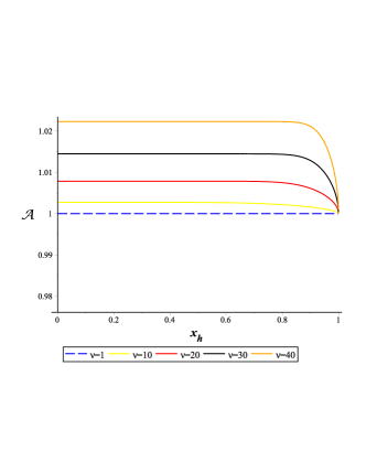
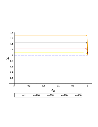
Figure 2: The left hand side graphic (c) describe (70) versus $x_{h}$ for the negative branch, we fix $a=2000~{}AU$ and $\alpha=2~{}AU^{-2}$. And according to our approximation $r_{g}/r<<1$ which means that $x_{h}<<1$. That is, in the graphic all these hairy black holes ($\nu>1$) have the same corrective factor, which is $\mathcal{A}>1$.
The right hand side graphic (d) describe (70) versus $x_{h}$ for the negative branch, we fix $a=2000~{}AU$ and $\alpha=2~{}AU^{-2}$. And according to our approximation $r_{g}/r<<1$ which means that $x_{h}<<1$. That is, in the graphic all these hairy black holes ($\nu>1$) have the same corrective factor, which is $\mathcal{A}>1$. But here the correction is larger than the previous case, because the hair is bigger.

Similar to Schwarzschild case, we can construct the eikonal equation, whose solution is

$$\psi=-\omega_{0}t+M\varphi+\psi_{x}$$ (71)

$$\psi_{x}=\frac{\omega_{0}}{c}\int{\sqrt{1-\varrho^{2}f}}\frac{\eta}{f}dx,\qquad\varrho=\frac{Mc}{\omega_{0}}$$ (72)

The equation of light trajectory is given by

$$\varphi(x)=\int\frac{\eta dx}{\sqrt{\frac{1}{\varrho^{2}}-f}}+cte$$ (74)

We need to consider the hairy-gravity corrections, considering one more time the coordinate transformations given in (66) we can show

$$\psi_{r}\approx\frac{\omega_{0}}{c}\int\sqrt{1+\frac{2r_{g}}{r}-\frac{\varrho_{\nu}^{2}}{r^{2}}}dr$$ (75)

where the impact parameter $\varrho$ has a new hairy correction

$$\varrho^{2}_{\nu}=\varrho^{2}+\frac{\nu^{2}-1}{4\eta^{2}}$$ (76)

Now, expanding around $r_{g}/r<<1$, keeping fix $\varrho_{\nu}^{2}/r^{2}$

$$\psi_{r}\approx\frac{\omega_{0}}{c}\int\sqrt{1-\frac{\varrho^{2}}{r^{2}}}dr+\frac{\omega_{0}r_{g}}{c}\int\frac{dr}{\sqrt{r^{2}-\varrho_{\nu}^{2}}}$$ (77)

In the first term of the expansion of $\psi_{r}$ we have $\sqrt{1-\frac{\varrho^{2}}{r^{2}}-\frac{\nu^{2}-1}{4\eta^{2}r^{2}}}\approx\sqrt{1-\frac{\varrho^{2}}{r^{2}}}$, this is because if we consider the horizon equation we have $\eta=\eta(x_{h},\alpha,\nu)$, and you can prove that for $x_{h}<<1$ ($r_{g}<<r$) we have $\eta^{2}$ large, then $\frac{3}{4r^{2}\eta^{2}}\approx 0$. But for the second term we have only $\sqrt{r^{2}-\varrho^{2}-\frac{\nu^{2}-1}{4\eta^{2}}}$, from which $\frac{\nu^{2}-1}{4\eta^{2}}$ is relevant. This is precisely the relevant hairy correction

$$\Delta\varphi=-\frac{\partial\Delta\psi_{r}^{(0)}}{\partial M}+\frac{2r_{g}Mc}{\omega_{0}\varrho_{\nu}^{2}}\frac{1}{\sqrt{1-\frac{\varrho_{\nu}^{2}}{R^{2}}}}$$ (78)

when $R\rightarrow\infty$

$$\Delta\varphi\approx\pi+\frac{2r_{g}}{\varrho}~{}\frac{\varrho^{2}}{\varrho_{\nu}^{2}}$$ (79)

And one more time when $\nu=1$ we obtain the Schwarzschild case giving in (33). Using the horizon equation $f(\eta,x_{h},\nu,\alpha)=0$ we have $\eta=\eta(x_{h},\nu,\alpha)$

$$\frac{\varrho_{\nu}^{2}}{\varrho^{2}}\biggr{|}_{(x_{h},\nu,\alpha)}=1+\frac{(\nu^{2}-1)}{4\eta^{2}\varrho^{2}}$$ (80)

To graph $\varrho^{2}/\varrho_{\nu}^{2}$ vs $x_{h}$, we consider $\varrho$ like multiples of $R_{\odot}$ (sun radius). For example the stars early-B hyper-giants (BHGs), has radios in the range of $\varrho=63.5R_{\odot}-246R_{\odot}$ Clark:2012ne . The figures in (3) show that the scalar field (hair) screening the effect of gravitational field, causing the deviation of light to be smaller respect to Schwarzschild case ($\nu=1$)

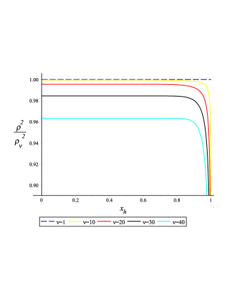
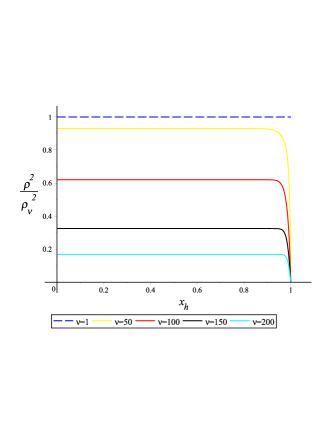
Figure 3: The left hand side graphic (e) describe (80) versus $x_{h}$ for the negative branch, we fix $\varrho=200R_{\odot}$ and $\alpha=10R_{\odot}^{-2}$. And according to our approximation $r_{g}/r<<1$ which means that $x_{h}<<1$, (see the graphic) all these hairy black holes ($\nu>1$) have the same screening factor, which is $\frac{\varrho^{2}}{\varrho_{\nu}^{2}}<1$.
The right hand side graphic (f) describe (80) versus $x_{h}$ for the negative branch, we fix $\varrho=200R_{\odot}$ and $\alpha=10R_{\odot}^{-2}$. And according to our approximation $r_{g}/r<<1$ which means that $x_{h}<<1$, (see the graphic) all these hairy black holes ($\nu>1$) have the same screening factor, which is $\frac{\varrho^{2}}{\varrho_{\nu}^{2}}<1$. But here the screening is larger than the previous case, because the hair is bigger.

5.2 Corrections of hairy solution $\nu=\infty$

We study the geodesics and null geodesics of the metric given in (44). Setting $\theta=\pi/2$, we have

$$ds^{2}=\Omega(x)\biggl{[}-c^{2}f(x)dt^{2}+\frac{\eta^{2}dx^{2}}{x^{2}f(x)}+d\varphi^{2}\biggr{]}$$ (81)

The Hamilton-Jacobi equation is

$$-\frac{1}{c^{2}\Omega f}\biggl{(}\frac{\partial I}{\partial t}\biggr{)}^{2}+\frac{x^{2}f}{\Omega\eta^{2}}\biggl{(}\frac{\partial I}{\partial x}\biggr{)}^{2}+\frac{1}{\Omega}\biggl{(}\frac{\partial I}{\partial\varphi}\biggr{)}^{2}+m^{2}c^{2}=0$$ (82)

the ansatz $I=-\mathcal{E}_{0}t+M\varphi+I_{x}(x)$, and the solution for $I_{x}(x)$ is

$$I_{x}=\int\sqrt{\frac{\eta^{2}}{x^{2}f^{2}}\biggl{(}\frac{\mathcal{E}_{0}}{c^{2}}-m^{2}c^{2}\Omega f\biggr{)}-\frac{\eta^{2}M^{2}}{x^{2}f}}~{}dx$$ (83)

Considering the coordinate transformation (49), and in a similar form to Schwarzschild case, we need to consider $r\rightarrow r+\frac{r_{g}}{2}$ and $\mathcal{E}_{0}=mc^{2}+\mathcal{E}^{{}^{\prime}}$, then, we can write $I_{x}$ like $I_{r}$ when $\frac{r_{g}}{r}<<1$

$$I_{r}=\int\sqrt{2m(E-U)+\frac{3\mathcal{A}m^{2}c^{2}r_{g}^{2}}{2r^{2}}-\frac{M^{2}}{r^{2}}+O\biggl{(}\frac{r_{g}^{3}}{r^{3}}\biggr{)}}~{}dr,\qquad\mathcal{A}=1-\frac{\mathcal{E}^{{}^{\prime}}}{mc^{2}\eta^{2}r_{g}^{2}}$$ (84)

Where the expressions for $E$, $U$ was given in (19). The new term $\mathcal{A}$ depend on constant integration $\eta$. We show that $\mathcal{A}$ give a hairy correction to periapsis shift. For these purpose we need expand (84) around $r_{g}/r<<1$ (keeping fix $M^{2}/r^{2}$) and $E\approx\mathcal{E}^{{}^{\prime}}$, $U\approx U_{N}$. And we have,

$$\Delta\varphi\approx 2\pi+\frac{3\pi m^{2}c^{2}r_{g}^{2}\mathcal{A}}{2M^{2}}$$ (85)

where the orbital parameter $a$ is the semi-major axis,

$$\mathcal{A}(a,\alpha,x_{h})=1+\frac{3\sqrt{\alpha}}{2a}~{}\sqrt{\frac{2x_{h}\ln{x_{h}}-x_{h}^{2}+1}{2(x_{h}-1)^{2}}}$$ (86)

In this case, there are not a hairy parameter such that $\mathcal{A}=1$, the unique form to obtain $\mathcal{A}=1$ is when $\alpha=0$, but according to (40) and (47), these case correspond to a naked singularity. Even if we consider black holes asymptotically AdS , the special case $\alpha=0$ is a naked singularity. Is clear that $\alpha$ has an important role to existence of regular horizon. The condition $\alpha\neq 0$ ensure the existence of scalar potentials given in (35), (36), and this means that if $\alpha=0$, there are not self-interaction of the scalar field that ensures its stability and at the same time, we have a naked singularity.

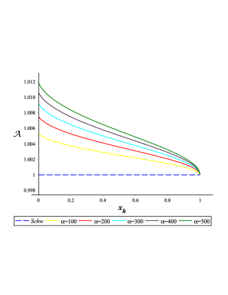
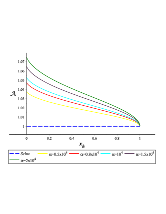
Figure 4: The left hand side graphic (g) describe (86) versus $x_{h}$ for the negative branch, we fix $a=2000~{}AU$ and $\alpha=(100-500)~{}AU^{-2}$. We put the case $Schw$ (Schwarzschild) to compare. And according to our approximation $r_{g}/r<<1$ which means that $x_{h}<<1$. That is, in the graphic all these hairy black holes have different (small) corrective factors, which is approximate $\mathcal{A}\sim 1$.
The right hand side graphic (h) describe (86) versus $x_{h}$ for the negative branch, we fix $a=2000~{}AU$ and $\alpha=(0.5-2)\times 10^{4}~{}AU^{-2}$. We put the case $Schw$ (Schwarzschild) to compare. And according to our approximation $r_{g}/r<<1$ which means that $x_{h}<<1$. That is, in the graphic, all these hairy black holes have different corrective factors. But here the correction is larger than the previous case because $\alpha$ is bigger.

To describe the light trajectory we use the eikonal equation. The ansatz is $\psi=-\omega_{0}t+M\varphi+\psi_{x}$, and the solution for $\psi_{x}$ is

$$\psi_{x}=\frac{\omega_{0}}{c}\int{\sqrt{1-\varrho^{2}f}}\frac{\eta}{xf}dx,\qquad\varrho=\frac{Mc}{\omega_{0}}$$ (87)

The equation of light trajectory is given by

$$\varphi(x)=\int\frac{\eta dx}{x\sqrt{1/\varrho^{2}-f}}+cte$$ (88)

But in here, we can not obtain the Schwarzschild as a smooth limit. To get the hairy-gravity corrections, we need to consider one more time the coordinate transformations given in (49) we can show, for $\frac{r_{g}}{r}<<1$

$$\psi_{r}\approx\frac{\omega_{0}}{c}\int\sqrt{1+\frac{2r_{g}}{r}-\frac{\varrho_{\alpha}^{2}}{r^{2}}}dr$$ (89)

where the impact parameter $\varrho$ has a new hairy term

$$\varrho^{2}_{\alpha}=\varrho^{2}+\frac{3}{4\eta^{2}}$$ (90)

Now, expanding around $r_{g}/r<<1$, keeping fix $\varrho_{\nu}^{2}/r^{2}$, we have

$$\psi_{r}\approx\frac{\omega_{0}}{c}\int\sqrt{1-\frac{\varrho^{2}}{r^{2}}}dr+\frac{\omega_{0}r_{g}}{c}\int\frac{dr}{\sqrt{r^{2}-\varrho_{\alpha}^{2}}}$$ (91)

In the first term of the expansion of $\psi_{r}$ we have $\sqrt{1-\frac{\varrho^{2}}{r^{2}}-\frac{3}{4\eta^{2}r^{2}}}\approx\sqrt{1-\frac{\varrho^{2}}{r^{2}}}$, this is because if we consider $\eta=\eta(x_{h},\alpha)$ given in (48), you can prove that for $x_{h}<<1$ ($r_{g}<<r$) we have $\eta^{2}$ large, then $\frac{3}{4r^{2}\eta^{2}}\approx 0$. But for the second term, we have only $\sqrt{r^{2}-\varrho^{2}-\frac{3}{4\eta^{2}}}$, from which $\frac{3}{4\eta^{2}}$ is not small enough. This is precisely the relevant hairy correction. Working in the same way as in the previous section, we can show that

$$\Delta\varphi=\pi+\frac{2r_{g}}{\varrho}~{}\frac{\varrho^{2}}{\varrho_{\alpha}^{2}};\qquad\frac{\varrho_{\alpha}^{2}}{\varrho^{2}}\biggr{|}_{(x_{h},\alpha)}=1+\frac{3}{2\alpha\varrho^{2}}~{}\frac{(x_{h}-1)^{2}}{2x_{h}\ln{x_{h}-x_{h}^{2}+1}}$$ (92)

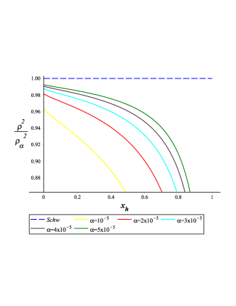
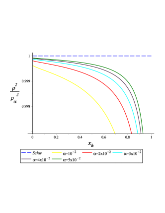
Figure 5: The left hand side graphic (i) describe (92) versus $x_{h}$ for the negative branch, we fix the impact parameter like $\varrho=2000R_{\odot}$. And according to our approximation $r_{g}/r<<1$ which means that $x_{h}<<1$, (see the graphic) these hairy black holes has different screening factors $\frac{\varrho^{2}}{\varrho_{\nu}^{2}}<1$, such that $\alpha\approx 0$.
The right-hand side graphic (k) describe (92) versus $x_{h}$ for the negative branch, we fix $\varrho=2000R_{\odot}$. And according to our approximation, $r_{g}/r<<1$ which means that $x_{h}<<1$, (see the graphic) these hairy black holes has small screening factor. Comparing with the before case, the screening is small, then $\frac{\varrho^{2}}{\varrho_{\nu}^{2}}\sim\frac{1}{\alpha}$ at fixed $\varrho$.

6 Conclusions

Sagittarius $A^{*}$ is a stellar system located in the center of our galaxy, it consists of a supermassive black hole, where until now the orbits of nine stars were studied Eisenhauer:2005cv ; Ghez:2003qj ; Ghez:1998ph ; Schodel:2002vg ; Clark:2012ne . This black hole has a disk accretion, and there are indications that dark matter influences the gravitational dynamics of these stars Ghez:1998ph . In 2004, source IRS 13 black hole was discovered (and other stars that orbit it) that orbit around of Sagittarius $A^{*}$. The principal idea of the present paper is that these hairy solutions (3.1) and (3.2) could be an effective model to describe a more complicated gravitational system. Our idea is to consider this gravitational system (for example Sagittarius $A^{*}$) as a black hole with scalar hair, specially the solution (3.1) has a hairy parameter $\nu$, it can be adjusted in such a way as to describe for example the Sagittarius $A^{*}$. We propose (like an elemental model) to use the results for periapsis shift given in (70), (85), and made astronomical observations to the stars that orbit Sagittarius $A^{*}$ , estimate its shift periapsis and thereby set the parameter of hair $\nu$ (and $\alpha$). In a similar form maybe is possible use the equation for deflection of light given in (80), (92). An interesting future direction is, study and classify the different orbits of these hairy black holes.

7 Acknowledgments

D. Choque would like to thank Dumitru Astefanesei for interesting discussions. D. Choque acknowledge the hospitality of the Universidad Nacional de San Antonio Abad del Cusco (UNSAAC) during the stages of this research. This work has been done with support from the 047-2017-FONDECYT-DE. The UNSAAC is funded by the Peruvian Government through Financing Program of CONCYTEC.

References

• (1) J. M. Maldacena, “The Large N limit of superconformal field theories and supergravity,” Adv. Theor. Math. Phys. 2, 231 (1998) [hep-th/9711200].
• (2) D. Martelli and W. Mueck, “Holographic renormalization and Ward identities with the Hamilton-Jacobi method,” Nucl. Phys. B 654, 248 (2003) doi:10.1016/S0550-3213(03)00060-9 [hep-th/0205061].
• (3) A. Batrachenko, J. T. Liu, R. McNees, W. A. Sabra and W. Y. Wen, “Black hole mass and Hamilton-Jacobi counterterms,” JHEP 0505, 034 (2005) doi:10.1088/1126-6708/2005/05/034 [hep-th/0408205].
• (4) J. de Boer, “The Holographic renormalization group,” Fortsch. Phys.  49, 339 (2001) doi:10.1002/1521-3978(200105)49:4/6¡339:: AID-PROP339,3.0.CO, 2-A [hep-th/0101026].
• (5) I. Heemskerk and J. Polchinski, “Holographic and Wilsonian Renormalization Groups,” JHEP 1106, 031 (2011) doi:10.1007/JHEP06(2011)031 [arXiv:1010.1264 [hep-th]].
• (6) G. Aad et al. [ATLAS Collaboration], “Observation of a new particle in the search for the Standard Model Higgs boson with the ATLAS detector at the LHC,” Phys. Lett. B 716, 1 (2012) doi:10.1016/j.physletb.2012.08.020 [arXiv:1207.7214 [hep-ex]].
• (7) D. N. Spergel et al. [WMAP Collaboration], “Wilkinson Microwave Anisotropy Probe (WMAP) three year results: implications for cosmology,” Astrophys. J. Suppl.  170, 377 (2007) doi:10.1086/513700 [astro-ph/0603449].
• (8) P. A. R. Ade et al. [Planck Collaboration], “Planck 2013 results. XXII. Constraints on inflation,” Astron. Astrophys.  571, A22 (2014) doi:10.1051/0004-6361/201321569 [arXiv:1303.5082 [astro-ph.CO]].
• (9) A. Anabalon, D. Astefanesei, D. Choque and C. Martinez, “Trace Anomaly and Counterterms in Designer Gravity,” JHEP 1603, 117 (2016) doi:10.1007/JHEP03(2016)117 [arXiv:1511.08759 [hep-th]].
• (10) M. Henneaux, C. Martinez, R. Troncoso and J. Zanelli, “Asymptotic behavior and Hamiltonian analysis of anti-de Sitter gravity coupled to scalar fields,” Annals Phys.  322, 824 (2007) doi:10.1016/j.aop.2006.05.002 [hep-th/0603185].
• (11) A. Anabalon, D. Astefanesei and R. Mann, “Exact asymptotically flat charged hairy black holes with a dilaton potential,” arXiv:1308.1693 [hep-th].
• (12) G. W. Gibbons, R. Kallosh and B. Kol, “Moduli, scalar charges, and the first law of black hole thermodynamics,” Phys. Rev. Lett.  77, 4992 (1996) doi:10.1103/PhysRevLett.77.4992 [hep-th/9607108].
• (13) D. Astefanesei, K. Goldstein and S. Mahapatra, “Moduli and (un)attractor black hole thermodynamics,” Gen. Rel. Grav.  40, 2069 (2008) doi:10.1007/s10714-008-0616-6 [hep-th/0611140].
• (14) G. W. Gibbons and K. -i. Maeda, “Black Holes and Membranes in Higher Dimensional Theories with Dilaton Fields,” Nucl. Phys. B 298, 741 (1988).
• (15) A. Anabalon and J. Oliva, “Exact Hairy Black Holes and their Modification to the Universal Law of Gravitation,” Phys. Rev. D 86, 107501 (2012) doi:10.1103/PhysRevD.86.107501 [arXiv:1205.6012 [gr-qc]].
• (16) A. Anabalon, “Exact Black Holes and Universality in the Backreaction of non-linear Sigma Models with a potential in (A)dS4,” arXiv:1204.2720 [hep-th].
• (17) A. Anabalon, “Exact Hairy Black Holes,” Springer Proc. Phys.  157, 3 (2014) doi:10.1007/978-3-319-06761-2 1 [arXiv:1211.2765 [gr-qc]].
• (18) D. Nunez, H. Quevedo and D. Sudarsky, “Black holes have no short hair,” Phys. Rev. Lett.  76, 571 (1996) doi:10.1103/PhysRevLett.76.571 [gr-qc/9601020].
• (19) S. Ferrara, R. Kallosh and A. Strominger, “N=2 extremal black holes,” Phys. Rev. D 52, R5412 (1995) doi:10.1103/PhysRevD.52.R5412 [hep-th/9508072].
• (20) A. Strominger, “Macroscopic entropy of N=2 extremal black holes,” Phys. Lett. B 383, 39 (1996) doi:10.1016/0370-2693(96)00711-3 [hep-th/9602111].
• (21) S. Ferrara and R. Kallosh, “Supersymmetry and attractors,” Phys. Rev. D 54, 1514 (1996) doi:10.1103/PhysRevD.54.1514 [hep-th/9602136].
• (22) C. Frye and C. J. Efthimiou, “Stringy Corrections to the Classical Tests of General Relativity,” arXiv:1306.4869 [hep-th].
• (23) N. Cruz, M. Olivares and J. R. Villanueva, “The Geodesic structure of the Schwarzschild anti-de Sitter black hole,” Class. Quant. Grav.  22, 1167 (2005) doi:10.1088/0264-9381/22/6/016 [gr-qc/0408016].
• (24) N. Cruz, M. Olivares, J. Saavedra and J. R. Villanueva, “Null geodesics in the Reissner-Nordstrom Anti-de Sitter black holes,” arXiv:1111.0924 [gr-qc].
• (25) J. D. Wells, “When effective theories predict: The Inevitability of Mercury’s anomalous perihelion precession,” Published in J.D. Wells, Effective Theories in Physics: From Planetary Orbits to Elementary Particle doi:10.1007/978-3-642-34892-14 [arXiv:1106.1568 [physics.hist-ph]].
• (26) E. Hackmann and C. Lammerzahl, “Geodesic equation in Schwarzschild- (anti-) de Sitter space-times: Analytical solutions and applications,” Phys. Rev. D 78, 024035 (2008) doi:10.1103/PhysRevD.78.024035 [arXiv:1505.07973 [gr-qc]].
• (27) M. Olivares, Y. Vásquez, J. R. Villanueva and F. Moncada, “Motion of particles on a $z=2$ Lifshitz black hole in 3+1 dimensions,” Celestial Mech. Dyn. Astron.  119, 207 (2014) doi:10.1007/s10569-014-9555-6 [arXiv:1306.5285 [gr-qc]].
• (28) C. Magnan, “Complete calculations of the perihelion precession of Mercury and the deflection of light by the Sun in general relativity,” arXiv:0712.3709 [gr-qc].
• (29) V. Perlick and O. Y. Tsupko, “Light propagation in a plasma on Kerr spacetime: Separation of the Hamilton-Jacobi equation and calculation of the shadow,” Phys. Rev. D 95, no. 10, 104003 (2017) doi:10.1103/PhysRevD.95.104003 [arXiv:1702.08768 [gr-qc]].
• (30) F. Correa, A. Faúndez and C. Martínez, “Rotating hairy black hole and its microscopic entropy in three spacetime dimensions,” Phys. Rev. D 87, no. 2, 027502 (2013) doi:10.1103/PhysRevD.87.027502 [arXiv:1211.4878 [hep-th]].
• (31) M. Natsuume and T. Okamura, “Entropy for asymptotically AdS(3) black holes,” Phys. Rev. D 62, 064027 (2000) doi:10.1103/PhysRevD.62.064027 [hep-th/9911062].
• (32) L. D. Landau, E.M. Lifshitz, Mecánica, Editorial Reverte, S.A, 1994.
• (33) L. D. Landau, E.M. Lifshitz, Teor´ıa Cl´asica de los Campos, Editorial Reverte, S.A, 1975.
• (34) M. Vasudevan and K. A. Stevens, “Integrability of particle motion and scalar field propagation in Kerr-(Anti) de Sitter black hole spacetimes in all dimensions,” Phys. Rev. D 72, 124008 (2005) doi:10.1103/PhysRevD.72.124008 [gr-qc/0507096].
• (35) R. Schodel et al., “A Star in a 15.2 year orbit around the supermassive black hole at the center of the Milky Way,” Nature [Nature 419, 694 (2002)] doi:10.1038/nature01121 [astro-ph/0210426].
• (36) A. Anabalon and D. Astefanesei, “On attractor mechanism of $AdS_{4}$ black holes,” Phys. Lett. B 727, 568 (2013) [arXiv:1309.5863 [hep-th]].
• (37) A. Anabalon and D. Astefanesei, “Black holes in $\omega$-defomed gauged $N=8$ supergravity,” Phys. Lett. B 732, 137 (2014) [arXiv:1311.7459 [hep-th]].
• (38) W. Israel, “Event horizons in static vacuum space-times,” Phys.Rev. 164 (1967) 1776–1779;
B. Carter, “Axisymmetric Black Hole Has Only Two Degrees of Freedom,” Phys.Rev.Lett. 26 (1971) 331–333;
R. H. Price, “Nonspherical perturbations of relativistic gravitational collapse. 1. Scalar and gravitational perturbations,” Phys.Rev. D5 (1972) 2419–2438;
R. H. Price, “Nonspherical Perturbations of Relativistic Gravitational Collapse. II. Integer-Spin, Zero-Rest-Mass Fields,” Phys.Rev. D5 (1972) 2439–2454;
S. W. Hawking, “Breakdown of Predictability in Gravitational Collapse,” Phys. Rev. D14 (1976) 2460–2473;
J. D. Bekenstein, ‘No Hair’: Twenty–five Years After, chapter in Proceedings of the Second International Andrei D. Sakharov Conference in Physics, edited by I. M. Dremin and A. M. Semikhatov (World Scientific, Singapore, 1997).
• (39) J. D. Bekenstein, “Novel “no-scalar-hair” theorem for black holes,” Phys. Rev. D 51, no. 12, R6608 (1995). doi:10.1103/PhysRevD.51.R6608
• (40) D. Sudarsky, “A Simple proof of a no hair theorem in Einstein Higgs theory,” Class. Quant. Grav. 12, 579 (1995). doi:10.1088/0264-9381/12/2/023;
D. Sudarsky and T. Zannias, “Spherical black holes cannot support scalar hair,” Phys. Rev. D 58, 087502 (1998) doi:10.1103/PhysRevD.58.087502 [gr-qc/9712083].
• (41) A. Aceña, A. Anabalón, D. Astefanesei and R. Mann, “Hairy planar black holes in higher dimensions,” JHEP 1401, 153 (2014) doi:10.1007/JHEP01(2014)153 [arXiv:1311.6065 [hep-th]].
• (42) A. Acena, A. Anabalon and D. Astefanesei, “Exact hairy black brane solutions in $AdS_{5}$ and holographic RG flows,” Phys. Rev. D 87, no. 12, 124033 (2013) doi:10.1103/PhysRevD.87.1240
• (43) C. Martinez and R. Troncoso, “Electrically charged black hole with scalar hair,” Phys. Rev. D 74, 064007 (2006) doi:10.1103/PhysRevD.74.064007 [hep-th/0606130].
• (44) B. de Wit and H. Nicolai, “Deformations of gauged SO(8) supergravity and supergravity in eleven dimensions,” JHEP 1305, 077 (2013) doi:10.1007/JHEP05(2013)077 [arXiv:1302.6219 [hep-th]].
• (45) G. Dall’Agata, G. Inverso and M. Trigiante, “Evidence for a family of SO(8) gauged supergravity theories,” Phys. Rev. Lett.  109, 201301 (2012) doi:10.1103/PhysRevLett.109.201301 [arXiv:1209.0760 [hep-th]].
• (46) V. Balasubramanian and P. Kraus, “A Stress tensor for Anti-de Sitter gravity,” Commun. Math. Phys. 208, 413 (1999) [hep-th/9902121].
• (47) A. Anabalon, D. Astefanesei and D. Choque, “On the thermodynamics of hairy black holes,” Phys. Lett. B 743, 154 (2015) [arXiv:1501.04252 [hep-th]].
• (48) A. Anabalon, D. Astefanesei and D. Choque, “Hairy AdS Solitons,” Phys. Lett. B 762, 80 (2016) doi:10.1016/j.physletb.2016.08.049 [arXiv:1606.07870 [hep-th]].
• (49) R. C. Myers, “Stress tensors and Casimir energies in the AdS / CFT correspondence,” Phys. Rev. D 60, 046002 (1999) doi:10.1103/PhysRevD.60
• (50) D. Astefanesei and E. Radu, “Quasilocal formalism and black ring thermodynamics,” Phys. Rev. D 73, 044014 (2006) doi:10.1103/PhysRevD.73.044014 [hep-th/0509144].
• (51) D. Astefanesei, R. B. Mann and C. Stelea, “Note on counterterms in asymptotically flat spacetimes,” Phys. Rev. D 75, 024007 (2007) doi:10.1103/PhysRevD.75.024007 [hep-th/0608037].
• (52) D. Astefanesei, R. B. Mann, M. J. Rodriguez and C. Stelea, “Quasilocal formalism and thermodynamics of asymptotically flat black objects,” Class. Quant. Grav.  27, 165004 (2010) doi:10.1088/0264-9381/27/16/165004 [arXiv:0909.3852 [hep-th]].
• (53) D. Astefanesei, M. J. Rodriguez and S. Theisen, “Thermodynamic instability of doubly spinning black objects,” JHEP 1008, 046 (2010) doi:10.1007/JHEP08(2010)046 [arXiv:1003.2421 [hep-th]].
• (54) J. D. Brown and J. W. York, Jr., “Quasilocal energy and conserved charges derived from the gravitational action,” Phys. Rev. D 47, 1407 (1993) doi:10.1103/PhysRevD.47.1407 [gr-qc/9209012].
• (55) F. Eisenhauer et al., “SINFONI in the Galactic Center: Young stars and IR flares in the central light month,” Astrophys. J.  628, 246 (2005) doi:10.1086/430667 [astro-ph/0502129].
• (56) A. M. Ghez, S. Salim, S. D. Hornstein, A. Tanner, M. Morris, E. E. Becklin and G. Duchene, “Stellar orbits around the galactic center black hole,” Astrophys. J.  620, 744 (2005) doi:10.1086/427175 [astro-ph/0306130].
• (57) A. M. Ghez, B. L. Klein, M. Morris and E. E. Becklin, “High proper motion stars in the vicinity of Sgr A*: Evidence for a supermassive black hole at the center of our galaxy,” Astrophys. J.  509, 678 (1998) doi:10.1086/306528 [astro-ph/9807210].
• (58) J. S. Clark, F. Najarro, I. Negueruela, B. W. Ritchie, M. A. Urbaneja and I. D. Howarth, “On the nature of the galactic early-B hypergiants,” Astron. Astrophys.  541 (2012) A145 doi:10.1051/0004-6361/201117472 [arXiv:1202.3991 [astro-ph.SR]].