Deep Learning for User Comment Moderation

Abstract

Experimenting with a new dataset of 1.6M user comments from a Greek news portal and existing datasets of English Wikipedia comments, we show that an rnn outperforms the previous state of the art in moderation. A deep, classification-specific attention mechanism improves further the overall performance of the rnn. We also compare against a cnn and a word-list baseline, considering both fully automatic and semi-automatic moderation.

1 Introduction

User comments play a central role in social media and online discussion fora. News portals and blogs often also allow their readers to comment in order to get feedback, engage their readers, and build customer loyalty. User comments, however, and more generally user content can also be abusive (e.g., bullying, profanity, hate speech). Social media are increasingly under pressure to combat abusive content. News portals also suffer from abusive user comments, which damage their reputation and make them liable to fines, e.g., when hosting comments encouraging illegal actions. They often employ moderators, who are frequently overwhelmed by the volume of comments. Readers are disappointed when non-abusive comments do not appear quickly online because of moderation delays. Smaller news portals may be unable to employ moderators, and some are forced to shut down their comments sections entirely.

We examine how deep learning Goodfellow et al. (2016); Goldberg (2016) can be used to moderate user comments. We experiment with a new dataset of approx. 1.6M manually moderated user comments from a Greek sports portal (Gazzetta), which we make publicly available. Furthermore, we provide word embeddings pre-trained on 5.2M comments from the same portal. We also experiment on the datasets of Wulczyn et al. Wulczyn et al. (2017), which contain English Wikipedia comments labeled for personal attacks, aggression, toxicity.

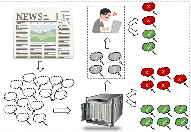
Figure 1: Semi-automatic moderation.

In a fully automatic scenario, a system directly accepts or rejects comments. Although this scenario may be the only available one, e.g., when portals cannot afford moderators, it is unrealistic to expect that fully automatic moderation will be perfect, because abusive comments may involve irony, sarcasm, harassment without profanity etc., which are particularly difficult for machines to handle. When moderators are available, it is more realistic to develop semi-automatic systems to assist rather than replace them, a scenario that has not been considered in previous work. Comments for which the system is uncertain (Fig. 1) are shown to a moderator to decide; all other comments are accepted or rejected by the system. We discuss how moderation systems can be tuned, depending on the availability and workload of moderators. We also introduce additional evaluation measures for the semi-automatic scenario.

On both Gazzetta and Wikipedia comments and for both scenarios (automatic, semi-automatic), we show that a recursive neural network (rnn) outperforms the system of Wulczyn et al. Wulczyn et al. (2017), the previous state of the art for comment moderation, which employed logistic regression (lr) or a multi-layered Perceptron (mlp). We also propose an attention mechanism that improves the overall performance of the rnn. Our attention differs from most previous ones Bahdanau et al. (2015); Luong et al. (2015) in that it is used in text classification, where there is no previously generated output subsequence to drive the attention, unlike sequence-to-sequence models Sutskever et al. (2014). In effect, our attention mechanism detects the words of a comment that affect mostly the classification decision (accept, reject), by examining them in the context of the particular comment.

Our main contributions are: (i) We release a new dataset of 1.6M moderated user comments. (ii) We are among the first to apply deep learning to user comment moderation, and we show that an rnn with a novel classification-specific attention mechanism outperforms the previous state of the art. (iii) Unlike previous work, we also consider a semi-automatic scenario, along with threshold tuning and evaluation measures for it.

2 Datasets

We first discuss the datasets we used, to help acquaint the reader with the problem.

Dataset/Split	Accepted	Rejected	Total
g-train-l	960,378 (66%)	489,222 (34%)	1,45M
g-train-s	67,828 (68%)	32,172 (32%)	100,000
g-dev	20,236 (68%)	9,464 (32%)	29,700
g-test-l	20,064 (68%)	9,636 (32%)	29,700
g-test-s	1,068 (71%)	432 (29%)	1,500
g-test-s-r	1,174 (78%)	326 (22%)	1,500
w-att-train	61,447 (88%)	8,079 (12%)	69,526
w-att-dev	20,405 (88%)	2,755 (12%)	23,160
w-att-test	20,422 (88%)	2,756 (12%)	23,178
w-tox-train	86,447 (90%)	9,245 (10%)	95,692
w-tox-dev	29,059 (90%)	3,069 (10%)	32,128
w-tox-test	28,818 (90%)	3,048 (10%)	31,866

Table 1: Statistics of the datasets used.

2.1 Gazzetta dataset

There are approx. 1.45M training comments (covering Jan. 1, 2015 to Oct. 6, 2016) in the Gazzetta dataset; we call them g-train-l (Table 1). Some experiments use only the first 100K comments of g-train-l, called g-train-s. An additional set of 60,900 comments (Oct. 7 to Nov. 11, 2016) was split to development (g-dev, 29,700 comments), large test (g-test-l, 29,700), and small test set (g-test-s, 1,500). Gazzetta’s moderators (2 full-time, plus journalists occasionally helping) are occasionally instructed to be stricter (e.g., during violent events). To get a more accurate view of performance in normal situations, we manually re-moderated (labeled as ‘accept’ or ‘reject’) the comments of g-test-s, producing g-test-s-r. The reject ratio is approximately 30% in all subsets, except for g-test-s-r where it drops to 22%, because there are no occasions where the moderators were instructed to be stricter in g-test-s-r.

Each g-test-s-r comment was re-moderated by 5 annotators. Krippendorff’s Krippendorff (2004) alpha was 0.4762, close to the value (0.45) reported by Wulczyn et al. Wulczyn et al. (2017) for Wikipedia comments. Using Cohen’s Kappa Cohen (1960), the mean pairwise agreement was 0.4749. The mean pairwise percentage of agreement (% of comments each pair of annotators agreed on) was 81.33%. Cohen’s Kappa and Krippendorff’s alpha lead to moderate scores, because they account for agreement by chance, which is high when there is class imbalance (22% reject, 78% accept in g-test-s-r).

We also provide 300-dimensional word embeddings, pre-trained on approx. 5.2M comments (268M tokens) from Gazzetta using word2vec Mikolov et al. (2013a, b). This larger dataset cannot be used to train classifiers, because most of its comments are from a period (before 2015) when Gazzetta did not employ moderators.

2.2 Wikipedia datasets

Wulczyn et al. Wulczyn et al. (2017) created three datasets containing English Wikipedia talk page comments.

Attacks dataset: This dataset contains approx. 115K comments, which were labeled as personal attacks (reject) or not (accept) using crowdsourcing. Each comment was labeled by at least 10 annotators. Inter-annotator agreement, measured on a random sample of 1K comments using Krippendorff’s Krippendorff (2004) alpha, was 0.45. The gold label of each comment is determined by the majority of annotators, leading to binary labels (accept, reject). Alternatively, the gold label is the percentage of annotators that labeled the comment as ‘accept’ (or ‘reject’), leading to probabilistic labels. The dataset is split in three parts (Table 1): training (w-att-train, 69,526 comments), development (w-att-dev, 23,160), and test (w-att-test, 23,178 comments). In all three parts, the rejected comments are 12%, but this ratio is artificial (in effect, Wulczyn et al. oversampled comments posted by banned users), unlike Gazzetta subsets where the truly observed accept/reject ratios are used.

Toxicity dataset: This dataset was created like the previous one, but contains more comments (159,686), now labeled as toxic (reject) or not (accept). Inter-annotator agreement was not reported. Again, binary or probabilistic gold labels can be used. The dataset is split in three parts (Table 1): training (w-tox-train, 95,692 comments), development (w-tox-dev, 32,128), and test (w-tox-test, 31,866). In all three parts, the rejected (toxic) comments are 10%, again an artificial ratio.

Wikipedia comments are longer (median 38 and 39 tokens for attacks, toxicity) compared to Gazzetta’s (median 25). Wulczyn et al. Wulczyn et al. (2017) also created an ‘aggression’ dataset containing the same comments as the personal attacks one, but now labeled as aggressive or not. The (probabilistic) labels of the two datasets are very highly correlated (0.8992 Spearman, 0.9718 Pearson) and we do not consider the aggression dataset further.

3 Methods

We experimented with an rnn operating on word embeddings, the same rnn enhanced with our attention mechanism (a-rnn), several variants of a-rnn, a vanilla convolutional neural network (cnn) also operating on word embeddings, the detox system of Wulczyn et al. Wulczyn et al. (2017), and a baseline that uses word lists with precision scores.

3.1 DETOX

detox Wulczyn et al. (2017) was the previous state of the art in comment moderation, in the sense that it had the best reported results on the Wikipedia datasets (Section 2.2), the largest previous publicly available datasets of moderated user comments. detox represents each comment as a bag of word $n$-grams ($n\leq 2$, each comment becomes a bag containing its 1-grams and 2-grams) or a bag of character $n$-grams ($n\leq 5$, each comment becomes a bag containing character 1-grams, …, 5-grams). detox can rely on a logistic regression (lr) or multi-layer Perceptron (mlp) classifier, and uses binary or probabilistic gold labels (Section 2.2) during training. We used the detox implementation of Wulczyn et al. and the same grid search to tune the hyper-parameters that select word or character $n$-grams, classifier (lr or mlp), and gold labels (binary or probabilistic). For Gazzetta, only binary gold labels were possible, since g-train-l and g-train-s have a single gold label per comment. Unlike Wulczyn et al., we tuned the hyper-parameters by evaluating (computing auc and Spearman, Section 4) on a random 2% of held-out comments of w-att-train, w-tox-train, or g-train-s, instead of the development subsets, to be able to obtain more realistic results from the development sets while developing the methods. The tuning always preferred character $n$-grams, as in the work of Wulczyn et al., and lr to mlp, whereas Wulczyn et al. reported slightly higher performance for the mlp on w-att-dev. The tuning also selected probabilistic labels when available (Wikipedia datasets), as in the work of Wulczyn et al.

3.2 RNN-based methods

rnn: The rnn method is a chain of gru cells Cho et al. (2014) that transforms the tokens $w_{1}\dots,w_{k}$ of each comment to hidden states $h_{1}\dots,h_{k}$, followed by an lr layer that uses $h_{k}$ to classify the comment (accept, reject). Formally, given the vocabulary $V$, a matrix $E\in\mathbb{R}^{d\times|V|}$ containing $d$-dimensional word embeddings, an initial $h_{0}$, and a comment $c=\left<w_{1},\dots,w_{k}\right>$, the rnn computes $h_{1},\dots,h_{k}$ as follows ($h_{t}\in\mathbb{R}^{m}$):

$$\tilde{h}_{t} = \tanh(W_{h}x_{t}+U_{h}(r_{t}\odot h_{t-1})+b_{h})$$

$$h_{t} = (1-z_{t})\odot h_{t-1}+z_{t}\odot\tilde{h}_{t}$$

$$z_{t} = \sigma(W_{z}x_{t}+U_{z}h_{t-1}+b_{z})$$

$$r_{t} = \sigma(W_{r}x_{t}+U_{r}h_{t-1}+b_{r})$$

where $\tilde{h}_{t}\in\mathbb{R}^{m}$ is the proposed hidden state at position $t$, obtained by considering the word embedding $x_{t}$ of token $w_{t}$ and the previous hidden state $h_{t-1}$; $\odot$ denotes element-wise multiplication; $r_{t}\in\mathbb{R}^{m}$ is the reset gate (for $r_{t}$ all zeros, it allows the rnn to forget the previous state $h_{t-1}$); $z_{t}\in\mathbb{R}^{m}$ is the update gate (for $z_{t}$ all zeros, it allows the rnn to ignore the new proposed $\tilde{h}_{t}$, hence also $x_{t}$, and copy $h_{t-1}$ as $h_{t}$); $\sigma$ is the sigmoid function; $W_{h},W_{z},W_{r}\in\mathbb{R}^{m\times d}$; $U_{h},U_{z},U_{r}\in\mathbb{R}^{m\times m}$; $b_{h},b_{z},b_{r}\in\mathbb{R}^{m}$. Once $h_{k}$ has been computed, the lr layer estimates the probability that comment $c$ should be rejected, with $W_{p}\in\mathbb{R}^{1\times m},b_{p}\in\mathbb{R}$:

$$P_{\textsc{rnn}}(\textit{reject}|c) = \sigma(W_{p}h_{k}+b_{p})$$

a-rnn: When the attention mechanism is added, the lr layer considers the weighted sum $h_{\textit{sum}}$ of all the hidden states, instead of just $h_{k}$ (Fig. 2):

$$h_{sum} = \sum_{t=1}^{k}a_{t}h_{t}$$ (1)

$$P_{\textit{a}-\textsc{rnn}}(\textit{reject}|c) = \sigma(W_{p}h_{\textit{sum}}+b_{p})$$

The weights $a_{t}$ are produced by an attention mechanism, which is an mlp with $l$ layers:

$$a_{t}^{(1)} = \textsc{r}e\textsc{lu}(W^{(1)}h_{t}+b^{(1)})$$

$$\dots$$

$$a_{t}^{(l-1)} = \textsc{r}e\textsc{lu}(W^{(l-1)}a_{t}^{(l-2)}+b^{(l-1)})$$

$$a_{t}^{(l)} = W^{(l)}a_{t}^{(l-1)}+b^{(l)}$$

$$a_{t} = \texttt{softmax}(a_{t}^{(l)};a_{1}^{(l)},\dots,a_{k}^{(l)})$$

where $a_{t}^{(1)},\dots,a_{t}^{(l-1)}\in\mathbb{R}^{r}$, $a_{t}^{(l)},a_{t}\in\mathbb{R}$, $W^{(1)}\in\mathbb{R}^{r\times m}$, $W^{(2)},\dots,W^{(l-1)}\in\mathbb{R}^{r\times r}$, $W^{(l)}\in\mathbb{R}^{1\times r}$, $b^{(1)},\dots,b^{(l-1)}\in\mathbb{R}^{r}$, $b^{(l)}\in\mathbb{R}$. The softmax operates across all the $a_{t}^{(l)}$ ($t=1,\dots,k$), making the attention weights $a_{t}$ sum to 1. Our attention mechanism differs from most previous ones Mnih et al. (2014); Bahdanau et al. (2015); Xu et al. (2015); Luong et al. (2015) in that it is used in a classification setting, where there is no previously generated output subsequence (e.g., partly generated translation) to drive the attention (e.g., assign more weight to source words to translate next), unlike seq2seq models Sutskever et al. (2014). It assigns larger weights $a_{t}$ to hidden states $h_{t}$ corresponding to positions where there is more evidence that the comment should be accepted or rejected.

Yang et al. Yang et al. (2016) use a similar attention mechanism, but ours is deeper. In effect they always set $l=2$, whereas we allow $l$ to be larger (tuning selects $l=4$). On the other hand, the attention mechanism of Yang et al. is part of a classification method for longer texts (e.g., product reviews). Their method uses two gru rnns, both bidirectional Schuster and Paliwal (1997), one turning the word embeddings of each sentence to a sentence embedding, and one turning the sentence embeddings to a document embedding, which is then fed to an lr layer. Yang et al. use their attention mechanism in both rnns, to assign attention scores to words and sentences. We consider shorter texts (comments), we have a single rnn, and we assign attention scores to words only.

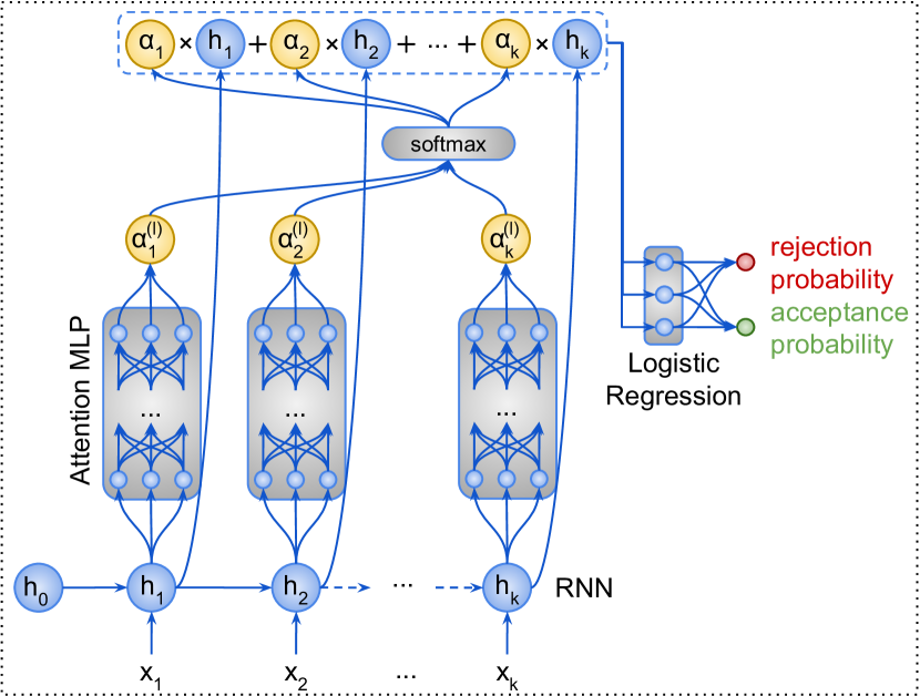
Figure 2: Illustration of a-rnn.

da-rnn: In a variant of a-rnn, called da-rnn (direct attention), the input to the first layer of the attention mechanism is the embedding $x_{t}$ of word $w_{t}$, rather than $h_{t}$ (cf. Eq. 3.2; $W^{(1,x)}\in\mathbb{R}^{r\times d}$):

$$a_{t}^{(1)}=\textsc{r}e\textsc{lu}(W^{(1,x)}x_{t}+b^{(1)})$$ (3)

Intuitively, the attention of a-rnn considers each word embedding $x_{t}$ in its (left) context, modelled by $h_{t}$, whereas the attention of da-rnn considers directly $x_{t}$ without its context, but $h_{\textit{sum}}$ is still the weighted sum of the hidden states (Eq. 1).

eq-rnn: In another variant of a-rnn, called eq-rnn, we assign equal attention to all the hidden states. The feature vector of the lr layer is now the average $h_{\textit{sum}}=\frac{1}{k}\sum_{t=1}^{k}h_{t}$ (cf. Eq. 1).

da-cent: For ablation testing, we also experiment with a variant, called da-cent, that does not use the hidden states of the rnn. The input to the attention mechanism is now directly the embedding $x_{t}$ instead of $h_{t}$ (as in da-rnn, Eq. 3), and $h_{\textit{sum}}$ is the weighted average (centroid) of word embeddings $h_{\textit{sum}}=\sum_{t=1}^{k}a_{t}x_{t}$ (cf. Eq. 1).

eq-cent: For further ablation, we also experiment with eq-cent, which uses neither the rnn nor the attention mechanism. The feature vector of the lr layer is now simply the average of word embeddings $h_{\textit{sum}}=\frac{1}{k}\sum_{t=1}^{k}x_{t}$ (cf. Eq. 1).

We set $l=4,d=300,m=r=128$, having tuned the hyper-parameters of rnn and a-rnn on the same 2% held-out training comments used to tune detox; da-rnn, eq-rnn, da-cent, and eq-cent use the same hyper-parameter values as a-rnn, to make their results more directly comparable and save time. We use Glorot initialization Glorot and Bengio (2010), cross-entropy loss, and Adam Kingma and Ba (2015). Early stopping evaluates on the same held-out subsets. For Gazzetta, word embeddings are initialized to the word2vec embeddings we provide (Section 2.1). For the Wikipedia datasets, they are initialized to glove embeddings Pennington et al. (2014). In both cases, the embeddings are updated during backpropagation. Out of vocabulary (oov) words, meaning words not encountered in the training set and/or words we have no initial embeddings for, are mapped (during training and testing) to a single randomly initialized embedding, which is also updated during training.

3.3 CNN

We also compare against a vanilla cnn operating on word embeddings. We describe the cnn only briefly, because it is very similar to that of of Kim Kim (2014); see also Goldberg Goldberg (2016) for an introduction to cnns, and Zhang and Wallace Zhang and Wallace (2015).

For Wikipedia comments, we use a ‘narrow’ convolution layer, with kernels sliding (stride 1) over (entire) embeddings of word $n$-grams of sizes $n=1,\dots,4$. We use 300 kernels for each $n$ value, a total of 1,200 kernels. The outputs of each kernel, obtained by applying the kernel to the different $n$-grams of a comment $c$, are then max-pooled, leading to a single output per kernel. The resulting feature vector (1,200 max-pooled outputs) goes through a dropout layer Hinton et al. (2012) ($p=0.5$), and then to an lr layer, which provides $P_{\textsc{cnn}}(\textit{reject}|c)$. For Gazzetta, the cnn is the same, except that $n=1,\dots,5$, leading to 1,500 features per comment. All hyper-parameters were tuned on the 2% held-out training comments used to tune the other methods. Again, we use 300-dimensional word embeddings, which are now randomly initialized, since tuning indicated this was better than initializing to pre-trained embeddings. oov words are treated as in the rnn-based methods. All embeddings are updated. Early stopping evaluates on the held-out subsets. Again, we use Glorot initialization, cross-entropy loss, and Adam.

3.4 LIST baseline

A baseline, called list, collects every word $w$ that occurs in more than 10 (for w-att-train, w-tox-train, g-train-s) or 100 comments (for g-train-l) in the training set, along with the precision of $w$, i.e., the ratio of rejected training comments containing $w$ divided by the total number of training comments containing $w$. The resulting lists contain 10,423, 11,360, 16,864, and 21,940 word types, when using w-att-train, w-tox-train, g-train-s, g-train-l, respectively. For a comment $c$, $P_{\textsc{list}}(\textit{reject}|c)$ is the maximum precision of all the words in $c$.

3.5 Tuning thresholds

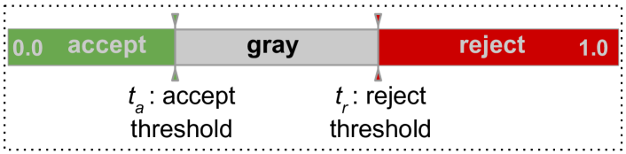
Figure 3: Illustration of threshold tuning.

All methods produce a $p=P(\textit{reject}|c)$ per comment $c$. In semi-automatic moderation (Fig. 1), a comment is directly rejected if its $p$ is above a rejection threshold $t_{r}$, it is directly accepted if $p$ is below an acceptance threshold $t_{a}$, and it is shown to a moderator if $t_{a}\leq p\leq t_{r}$ (gray zone of Fig. 3).

In our experience, moderators (or their employers) can easily specify the approximate percentage of comments they can afford to check manually (e.g., 20% daily) or, equivalently, the approximate percentage of comments the system should handle automatically. We call coverage the latter percentage; hence, $1-\textit{coverage}$ is the approximate percentage of comments to be checked manually. By contrast, moderators are baffled when asked to tune $t_{r}$ and $t_{a}$ directly. Consequently, we ask them to specify the approximate desired coverage. We then sort the comments of the development set (g-dev, w-att-dev, w-tox-dev) by $p$, and slide $t_{a}$ from $0.0$ to $1.0$ (Fig. 3). For each $t_{a}$ value, we set $t_{r}$ to the value that leaves a $1-\textit{coverage}$ percentage of development comments in the gray zone ($t_{a}\leq p\leq t_{r}$). We then select the $t_{a}$ (and $t_{r}$) that maximizes the weighted harmonic mean $F_{\beta}(P_{\textit{reject}},P_{\textit{accept}})$ on the development set:

$$F_{\beta}(P_{\textit{reject}},P_{\textit{accept}})=\frac{(1+{\beta}^{2})\cdot P_{\textit{reject}}\cdot P_{\textit{accept}}}{{\beta}^{2}\cdot P_{\textit{reject}}+P_{\textit{accept}}}$$

where $P_{\textit{reject}}$ is the rejection precision (correctly rejected comments divided by rejected comments) and $P_{\textit{accept}}$ is the acceptance precision (correctly accepted divided by accepted). Intuitively, coverage sets the width of the gray zone, whereas $P_{\textit{reject}}$ and $P_{\textit{accept}}$ show how certain we can be that the red (reject) and green (accept) zones are free of misclassified comments. We set $\beta=2$, emphasizing $P_{\textit{accept}}$, because moderators are more worried about wrongly accepting abusive comments than wrongly rejecting non-abusive ones. The selected $t_{a},t_{r}$ (tuned on development data) are then used in experiments on test data. In fully automatic moderation, $\textit{coverage}=100\%$ and $t_{a}=t_{r}$; otherwise, threshold tuning is identical.

4 Experimental results

Following Wulczyn et al. Wulczyn et al. (2017), we report in Tables 2–3 auc scores (area under roc curve), along with Spearman correlations between system-generated probabilities $P(\textit{accept}|c)$ and human probabilistic gold labels (Section 2.2) when probabilistic gold labels are available.

Training dataset: g-train-s
System	g-dev	g-test-l	g-test-s	g-test-s-r
	auc	auc	auc	auc	Spearman
rnn	75.75	75.10	74.40	80.27	51.89
a-rnn	76.19	76.15	75.83	80.41	52.51
da-rnn	75.96	75.90	74.25	80.05	52.49
eq-rnn	74.31	74.01	73.28	77.73	45.77
da-cent	75.09	74.96	74.20	79.92	51.04
eq-cent	73.93	73.82	73.80	78.45	48.14
cnn	70.97	71.34	70.88	76.03	42.88
detox	72.50	72.06	71.59	75.67	43.80
list	61.47	61.59	61.26	64.19	24.33
Training dataset: g-train-l
System	g-dev	g-test-l	g-test-s	g-test-s-r
	auc	auc	auc	auc	Spearman
rnn	79.50	79.41	79.23	84.17	59.31
a-rnn	79.64	79.58	79.67	84.69	60.87
da-rnn	79.60	79.56	79.38	84.40	60.83
eq-rnn	77.45	77.76	77.28	82.11	55.01
da-cent	78.73	78.64	78.62	83.53	57.82
eq-cent	76.76	76.85	76.30	82.38	53.28
cnn	77.57	77.35	78.16	83.98	55.90
detox	–	–	–	–	–
list	67.04	67.06	66.17	69.51	33.61

Table 2: Results on Gazzetta comments.

A first observation is that increasing the size of the Gazzetta training set (g-train-s to g-train-l, Table 2) significantly improves the performance of all methods; we do not report detox results for g-train-l, because its implementation could not handle the size of g-train-l. Tables 2–3 also show that rnn is always better than cnn and detox; there is no clear winner between cnn and detox. Furthermore, a-rnn is always better than rnn on Gazzetta comments (Table 2), but not always on Wikipedia comments (Table 3). Another observation is that da-rnn is always worse than a-rnn (Tables 2–3), confirming that the hidden states of the rnn are a better input to the attention mechanism than word embeddings. The performance of da-rnn deteriorates further when equal attention is assigned to the hidden states (eq-rnn), when the weighted sum of hidden states ($h_{\textit{sum}}$) is replaced by the weighted sum of word embeddings (da-cent), or both (eq-cent). Also, da-cent outperforms eq-cent, indicating that the attention mechanism improves the performance of simply averaging word embeddings. The Wikipedia subsets are easier (all methods perform better on Wikipedia subsets, compared to Gazzetta).

Training dataset: w-att-train
System	w-att-dev		w-att-test
	auc	Spearman	auc	Spearman
rnn	97.39	71.92	97.71	72.79
a-rnn	97.46	71.59	97.68	72.32
da-rnn	97.02	71.49	97.31	72.11
eq-rnn	92.66	60.77	92.85	60.16
da-cent	96.73	70.13	97.06	71.08
eq-cent	92.30	57.21	92.81	56.33
cnn	96.91	70.06	97.07	70.21
detox	96.26	67.75	96.71	68.09
list	93.05	55.39	92.91	54.55
Training dataset: w-tox-train
System	w-tox-dev		w-tox-test
	auc	Spearman	auc	Spearman
rnn	98.20	68.84	98.42	68.89
a-rnn	98.22	68.95	98.38	68.90
da-rnn	98.05	68.59	98.28	68.55
eq-rnn	94.72	55.48	95.04	55.86
da-cent	97.83	67.86	97.94	67.74
eq-cent	94.31	53.35	94.61	52.93
cnn	97.76	65.50	97.86	65.56
detox	97.16	63.57	97.13	63.24
list	93.96	51.35	93.95	51.18

Table 3: Results on Wikipedia comments.

Figure 4 shows $F_{2}(P_{\textit{reject}},P_{\textit{accept}})$ on g-test-l, g-test-s, w-att-test, w-tox-test, when $t_{a},t_{r}$ are tuned on the corresponding development tests for varying coverage. For the Gazzetta datasets, we show results training on g-train-s (solid lines) and g-train-l (dashed). The differences between rnn and a-rnn are again small, but it is now easier to see that a-rnn is overall better. Again, a-rnn and rnn are better than cnn and detox, and the results improve with a larger training set (dashed). On w-att-test and w-tox-test, a-rnn obtains $P_{\textit{accept}},P_{\textit{reject}}\geq 0.94$ for all coverages (Fig. 4, call-outs). On the more difficult Gazzetta datasets, a-rnn still obtains $P_{\textit{accept}},P_{\textit{reject}}\geq 0.85$ when tuned for 50% coverage. When tuned for 100% coverage, comments for which the system is uncertain (gray zone) cannot be avoided and there are inevitably more misclassifications; the use of $F_{2}$ during threshold tuning places more emphasis on avoiding wrongly accepted comments, leading to high $P_{\textit{accept}}$ ($\geq 0.82$), at the expense of wrongly rejected comments, i.e., sacrificing $P_{\textit{reject}}$ ($\geq 0.56$). On the re-moderated g-test-s-r (similar diagrams, not shown), $P_{\textit{accept}},P_{\textit{reject}}$ become 0.96, 0.88 for coverage 50%, and 0.92, 0.48 for coverage 100%.

Figure 4: $F_{2}$ scores for varying coverage. Dashed lines were obtained using a larger training set.

5 Related work

Napoles et al. Napoles et al. (2017b) developed an annotation scheme for online conversations, with 6 dimensions for comments (e.g., sentiment, tone, off-topic) and 3 dimensions for threads. The scheme was used to label a dataset, called ynacc, of 9.2K comments (2.4K threads) from Yahoo News and 16.6K comments (1K threads) from the Internet Argument Corpus Walker et al. (2012); Abbott et al. (2016). Abusive comments were filtered out, hence ynacc cannot be used for our purposes, but it may be possible to extend the annotation scheme for abusive comments, to predict more fine-grained labels, instead of ‘accept’ or ‘reject’. Napoles et al. also reported that up/down votes, a form of social filtering, are inappropriate proxies for comment and thread quality. Lee et al. Lee et al. (2014) discuss social filtering in detail and propose features (e.g., thread depth, no. of revisiting users) to assess the quality of a thread without processing the texts of its comments. Diakopoulos Diakopoulos (2015) discusses how editors select high quality comments.

In further work, Napoles et al. Napoles et al. (2017a) aimed to identify high quality threads. Their best method converts each comment to a comment embedding using doc2vec Le and Mikolov (2014). An ensemble of Conditional Random Fields (crfs) Lafferty et al. (2001) assigns labels (from their annotation scheme, e.g., for sentiment, off-topic) to the comments of each thread, viewing each thread as a sequence of doc2vec embeddings. The decisions of the crfs are then used to convert each thread to a feature vector (total count and mean marginal probability of each label in the thread), which is passed on to an lr classifier. Further improvements were observed when additional features were added, bow counts and pos $n$-grams being the most important ones. Napoles et al. Napoles et al. (2017a) also experimented with a cnn, similar to that of Section 3.3, which was not however a top-performer, presumably because of the small size of the training set (2.1K ynacc threads).

Djuric et al. Djuric et al. (2015) experimented with 952K manually moderated comments from Yahoo Finance, but their dataset is not publicly available. They convert each comment to a doc2vec embedding, which is fed to an lr classifier. Nobata et al. Nobata et al. (2016) experimented with approx. 3.3M manually moderated comments from Yahoo Finance and News; their data are also not available. They used Vowpal Wabbit with character $n$-grams ($n=3,\dots,5$) and word $n$-grams ($n=1,2$), hand-crafted features (e.g., comment length, number of capitalized or black-listed words), features based on dependency trees, averages of word2vec embeddings, and doc2vec-like embeddings. Character $n$-grams were the best, on their own outperforming Djuric et al. Djuric et al. (2015). The best results, however, were obtained using all features. By contrast, we use no hand-crafted features and parsers, making our methods easily portable to other domains and languages.

Wulczyn et al. Wulczyn et al. (2017) experimented with character and word $n$-grams, based on the findings of Nobata et al. Nobata et al. (2016). We included their dataset and moderation system (detox) in our experiments. Wulczyn et al. also used detox (trained on w-att-train) as a proxy (instead of human annotators) to automatically classify 63M Wikipedia comments, which were then used to study the problem of personal attacks (e.g., the effect of allowing anonymous comments, how often personal attacks were followed by moderation actions). Our methods could replace detox in studies of this kind, since they perform better.

Waseem et al. Waseem and Hovy (2016) used approx. 17K tweets annotated for hate speech. Their best method was an lr classifier with character $n$-grams ($n=1,\dots,4$) and a gender feature. Badjatiya et al. Badjatiya et al. (2017) experimented with the same dataset using lr, svms Cortes and Vapnik (1995), Random Forests Ho (1995), Gradient Boosted Decision Trees (gbdt) Friedman (2002), cnn (similar to that of Section 3.3), lstm Greff et al. (2015), FastText Joulin et al. (2017). They also considered alternative feature sets: character $n$-grams, tf-idf vectors, word embeddings, averaged word embeddings. Their best results were obained using gbdt with averaged word embeddings learned by the lstm, starting from random embeddings.

Warner and Hirschberg Warner and Hirschberg (2012) aimed to detect anti-semitic speech, experimenting with 9K paragraphs and a linear svm. Their features consider windows of up to 5 tokens, the tokens of each window, their order, pos tags, Brown clusters etc., following Yarowsky Yarowsky (1994).

Cheng et al. Cheng et al. (2015) predict which users would be banned from on-line communities. Their best system uses a Random Forest or lr classifier, with features examining readability, activity (e.g., number of posts daily), community and moderator reactions (e.g., up-votes, number of deleted posts).

Lukin and Walker Lukin and Walker (2013) experimented with 5.5K utterances from the Internet Argument Corpus Walker et al. (2012); Abbott et al. (2016) annotated with nastiness scores, and 9.9K utterances from the same corpus annotated for sarcasm. In a bootstrapping manner, they manually identified cue words and phrases (indicative of nastiness or sarcasm), used the cue words to obtain training comments, and extracted patterns from the training comments. Xiang et al. Xiang et al. (2012) also employed bootstrapping to identify users whose tweets frequently or never contain profane words, and collected 381M tweets from the two user types. They trained decision tree, Random Forest, or lr classifiers to distinguish between tweets from the two user types, testing on 4K tweets manually labeled as containing profanity or not. The classifiers used topical features, obtained via lda Blei et al. (2003), and a feature indicating the presence of at least one of approx. 330 known profane words.

Sood et al. Sood et al. (2012a, b) experimented with 6.5K comments from Yahoo Buzz, moderated via crowdsourcing. They showed that a linear svm, representing each comment as a bag of word bigrams and stems, performs better than word lists. Their best results were obtained by combining the svm with a word list and edit distance.

Yin et al. Yin et al. (2009) used posts from chat rooms and discussion fora ($<$15K posts in total) to train an svm to detect online harassment. They used tf-idf, sentiment, and context features (e.g., similarity to other posts in a thread). Our methods might also benefit by considering threads, rather than individual comments. Yin et al. point out that unlike other abusive content, spam in comments or discussion fora Mishne et al. (2005); Niu et al. (2007) is off-topic and serves a commercial purpose. Spam is unlikely in Wikipedia discussions and extremely rare so far in Gazzetta comments.

Mihaylov and Nakov Mihaylov and Nakov (2016) identify comments posted by opinion manipulation trolls. Dinakar et al. Dinakar et al. (2011) and Dadvar et al. Dadvar et al. (2013) detect cyberbullying. Chandrinos et al. Chandrinos et al. (2000) detect pornographic web pages, using a Naive Bayes classifier with text and image features. Spertus Spertus (1997) flag flame messages in Web feedback forms, using decision trees and hand-crafted features. A Kaggle dataset for insult detection is also available. It contains 6.6K comments (3,947 train, 2,647 test) labeled as insults or not. However, abusive comments that do not directly insult other participants of the same discussion are not classified as insults, even if they contain profanity, hate speech, insults to third persons etc.

6 Conclusions

We experimented with a new publicly available dataset of 1.6M moderated user comments from a Greek sports news portal and two existing datasets of English Wikipedia talk page comments. We showed that a gru rnn operating on word embeddings outperforms the previous state of the art, which used an lr or mlp classifier with character or word $n$-gram features. It also outperforms a vanilla cnn operating on word embeddings, and a baseline that uses an automatically constructed word list with precision scores. A novel, deep, classification-specific attention mechanism improves further the overall results of the rnn. The attention mechanism also improves the results of a simpler method that averages word embeddings. We considered both fully automatic and semi-automatic moderation, along with threshold tuning and evaluation measures for both.

We plan to consider user-specific information (e.g., ratio of comments rejected in the past) and thread statistics (e.g., thread depth, number of revisiting users) Dadvar et al. (2013); Lee et al. (2014); Cheng et al. (2015); Waseem and Hovy (2016). We also plan to explore character-level rnns or cnns Zhang et al. (2015), for example to produce embeddings of unknown or obfuscated words from characters dos Santos and Zadrozny (2014); Ling et al. (2015). We are also exploring how the attention scores of a-rnn can be used to highlight ‘suspicious’ words or phrases when showing gray comments to moderators.

References

- Abbott et al. (2016) R. Abbott, B. Ecker, P. Anand, and M. A. Walker. 2016. Internet Argument Corpus 2.0: An SQL schema for dialogic social media and the corpora to go with it. In LREC. Portoroz, Slovenia.
- Badjatiya et al. (2017) P. Badjatiya, S. Gupta, M. Gupta, and V. Varma. 2017. Deep learning for hate speech detection in tweets. In WWW (Companion). Perth, Australia, pages 759–760.
- Bahdanau et al. (2015) D. Bahdanau, K. Cho, and Y. Bengio. 2015. Neural machine translation by jointly learning to align and translate. In ICLR. San Diego, CA.
- Blei et al. (2003) D. M. Blei, A. Y. Ng, and M. I. Jordan. 2003. Latent Dirichlet Allocation. Journal of Machine Learning Research 3:993–1022.
- Chandrinos et al. (2000) K.V. Chandrinos, I. Androutsopoulos, G. Paliouras, and C.D. Spyropoulos. 2000. Automatic Web rating: Filtering obscene content on the Web. In Proc. of the 4th European Conference on Research and Advanced Technology for Digital Libraries. Lisbon, Portugal, pages 403–406.
- Cheng et al. (2015) J. Cheng, C. Danescu-Niculescu-Mizil, and J. Leskovec. 2015. Antisocial behavior in online discussion communities. In Proc. of the International AAAI Conference on Web and Social Media. Oxford University, England, pages 61–70.
- Cho et al. (2014) K. Cho, B. van Merrienboer, C. Gulcehre, D. Bahdanau, F. Bougares, H. Schwenk, and Y. Bengio. 2014. Learning phrase representations using RNN encoder–decoder for statistical machine translation. In EMNLP. Doha, Qatar, pages 1724–1734.
- Cohen (1960) J. Cohen. 1960. A coefficient of agreement for nominal scales. Educational and Psychological Measurement 20(1):37–46.
- Cortes and Vapnik (1995) C. Cortes and Vladimir Vapnik. 1995. Support-Vector Networks. Machine Learning 20(3):273–297.
- Dadvar et al. (2013) M. Dadvar, D. Trieschnigg, R. Ordelman, and F. de Jong. 2013. Improving cyberbullying detection with user context. In ECIR. Moscow, Russia, pages 693–696.
- Davidov et al. (2010) D. Davidov, O. Tsur, and A. Rappoport. 2010. Semi-supervised recognition of sarcastic sentences in Twitter and Amazon. In CoNLL. Uppsala, Sweden, pages 107–116.
- Diakopoulos (2015) N. Diakopoulos. 2015. Picking the NYT picks: Editorial criteria and automation in the curation of online news comments. Journal of the International Symposium on Online Journalism 5:147–166.
- Dinakar et al. (2011) K. Dinakar, R. Reichart, and H. Lieberman. 2011. Modeling the detection of textual cyberbullying. In The Social Mobile Web. Barcelona, Spain, volume WS-11-02 of AAAI Workshops, pages 11–17.
- Djuric et al. (2015) N. Djuric, J. Zhou, R. Morris, M. Grbovic, V. Radosavljevic, and N. Bhamidipati. 2015. Hate speech detection with comment embeddings. In WWW. Florence, Italy, pages 29–30.
- dos Santos and Zadrozny (2014) C. N. dos Santos and B. Zadrozny. 2014. Learning character-level representations for part-of-speech tagging. In ICML. Beijing, China, pages 1818–1826.
- Friedman (2002) J.H. Friedman. 2002. Stochastic gradient boosting. Computational Statistics and Data Analysis 38(4):367–378.
- Glorot and Bengio (2010) X. Glorot and Y. Bengio. 2010. Understanding the difficulty of training deep feedforward neural networks. In Proc. of the International Conference on Artificial Intelligence and Statistics. Sardinia, Italy, pages 249–256.
- Goldberg (2016) Y. Goldberg. 2016. A primer on neural network models for natural language processing. Journal of Artificial Intelligence Research 57:345–420.
- González-Ibáñez et al. (2011) R. I. González-Ibáñez, S. Muresan, and N. Wacholder. 2011. Identifying sarcasm in Twitter: A closer look. In ACL. Portland, Oregon, pages 581–586.
- Goodfellow et al. (2016) I. Goodfellow, Y. Bengio, and A. Courville. 2016. Deep Learning. MIT Press.
- Greff et al. (2015) K. Greff, R.K. Srivastava, J. Koutník, B.R. Steunebrink, and J. Schmidhuber. 2015. LSTM: A search space Odyssey. CoRR abs/1503.04069.
- Hinton et al. (2012) G. E. Hinton, N. Srivastava, A. Krizhevsky, I. Sutskever, and R. Salakhutdinov. 2012. Improving neural networks by preventing co-adaptation of feature detectors. CoRR abs/1207.0580.
- Ho (1995) T.K. Ho. 1995. Random Decision Forests. In Proc. of the 3rd International Conference on Document Analysis and Recognition. Montreal, Canada, volume 1, pages 278–282.
- Joshi et al. (2015) A. Joshi, V. Sharma, and P. Bhattacharyya. 2015. Harnessing context incongruity for sarcasm detection. In ACL. Beijing, China, pages 757–762.
- Joulin et al. (2017) A. Joulin, E. Grave, P. Bojanowski, and T. Mikolov. 2017. Bag of tricks for efficient text classification. In EACL (short papers). Valencia, Spain, pages 427–431.
- Kim (2014) Y. Kim. 2014. Convolutional neural networks for sentence classification. In EMNLP. Doha, Qatar, pages 1746–1751.
- Kingma and Ba (2015) D. P. Kingma and J. Ba. 2015. Adam: A method for stochastic optimization. In ICLR. San Diego, CA.
- Krippendorff (2004) K. Krippendorff. 2004. Content Analysis: An Introduction to Its Methodology (2nd edition). Sage Publications.
- Lafferty et al. (2001) J. D. Lafferty, A. McCallum, and F. C. N. Pereira. 2001. Conditional Random Fields: Probabilistic models for segmenting and labeling sequence data. In ICML. Williamstown, MA, pages 282–289.
- Le and Mikolov (2014) Q. V. Le and T. Mikolov. 2014. Distributed representations of sentences and documents. In ICML. Beijing, China, pages 1188–1196.
- Lee et al. (2014) J.-T. Lee, M.-C. Yang, and H.-C. Rim. 2014. Discovering high-quality threaded discussions in online forums. Journal of Computer Science and Technology 29(3):519–531.
- Ling et al. (2015) W. Ling, C. Dyer, A. W. Black, I. Trancoso, R. Fermandez, S. Amir, L. Marujo, and T. Luís. 2015. Finding function in form: Compositional character models for open vocabulary word representation. In EMNLP. Lisbon, Portugal, pages 1520–1530.
- Liu (2015) B. Liu. 2015. Sentiment Analysis – Mining Opinions, Sentiments, and Emotions. Cambridge University Press.
- Lukin and Walker (2013) S. Lukin and M. Walker. 2013. Really? well. apparently bootstrapping improves the performance of sarcasm and nastiness classifiers for online dialogue. In Proc. of the Workshop on Language in Social Media. Atlanta, Georgia, pages 30–40.
- Luong et al. (2015) T. Luong, H. Pham, and C. D. Manning. 2015. Effective approaches to attention-based neural machine translation. In EMNLP. Lisbon, Portugal, pages 1412–1421.
- Mihaylov and Nakov (2016) T. Mihaylov and P. Nakov. 2016. Hunting for troll comments in news community forums. In ACL. Berlin, Germany, pages 399–405.
- Mikolov et al. (2013a) T. Mikolov, K. Chen, G. Corrado, and J. Dean. 2013a. Efficient estimation of word representations in vector space. In ICLR. Scottsdale, AZ.
- Mikolov et al. (2013b) T. Mikolov, W.-t. Yih, and G. Zweig. 2013b. Linguistic regularities in continuous space word representations. In NAACL-HLT. Atlanta, GA, pages 746–751.
- Mishne et al. (2005) G. Mishne, D. Carmel, and R. Lempel. 2005. Blocking blog spam with language model disagreement. In Proc. of the International Workshop on Adversarial Information Retrieval on the Web. Chiba, Japan.
- Mnih et al. (2014) V. Mnih, N. Heess, A. Graves, and K. Kavukcuoglu. 2014. Recurrent models of visual attention. In NIPS. Montreal, Canada, pages 2204–2212.
- Napoles et al. (2017a) C. Napoles, A. Pappu, and J. Tetreault. 2017a. Automatically identifying good conversations online (yes, they do exist!). In Proc. of the International AAAI Conference on Web and Social Media.
- Napoles et al. (2017b) C. Napoles, J. Tetreault, E. Rosato, B. Provenzale, and A. Pappu. 2017b. Finding good conversations online: The Yahoo News annotated comments corpus. In Proc. of the Linguistic Annotation Workshop. Valencia, Spain, pages 13–23.
- Niu et al. (2007) Y. Niu, Y.-M. Wang, H. Chen, M. Ma, and F. Hsu. 2007. A quantitative study of forum spamming using context-based analysis. In Proc. of the Annual Network and Distributed System Security Symposium. San Diego, CA, pages 79–92.
- Nobata et al. (2016) C. Nobata, J. Tetreault, A. Thomas, Y. Mehdad, and Y. Chang. 2016. Abusive language detection in online user content. In WWW. Montreal, Canada, pages 145–153.
- Oraby et al. (2016) S. Oraby, V. Harrison, L. Reed, E. Hernandez, E. Riloff, and M. A. Walker. 2016. Creating and characterizing a diverse corpus of sarcasm in dialogue. In SIGDial. Los Angeles, CA, pages 31–41.
- Pang and Lee (2008) B. Pang and L. Lee. 2008. Opinion mining and sentiment analysis. Foundations and Trends in Information Retrieval 2(1-2):1–135.
- Pennington et al. (2014) J. Pennington, R. Socher, and C. Manning. 2014. GloVe: Global vectors for word representation. In EMNLP. Doha, Qatar, pages 1532–1543.
- Schuster and Paliwal (1997) M. Schuster and K. K. Paliwal. 1997. Bidirectional recurrent neural networks. IEEE Transacions of Signal Processing 45(11):2673–2681.
- Sood et al. (2012a) S. Sood, J. Antin, and E. F. Churchill. 2012a. Profanity use in online communities. In SIGCHI. Austin, TX, pages 1481–1490.
- Sood et al. (2012b) S. Sood, J. Antin, and E. F. Churchill. 2012b. Using crowdsourcing to improve profanity detection. In AAAI Spring Symposium: Wisdom of the Crowd. Stanford, CA, pages 69–74.
- Spertus (1997) E. Spertus. 1997. Smokey: Automatic recognition of hostile messages. In Proc. of the National Conference on Artificial Intelligence and the Innovative Applications of Artificial Intelligence Conference. Providence, Rhode Island, pages 1058–1065.
- Sutskever et al. (2014) I. Sutskever, O. Vinyals, and Q. V. Le. 2014. Sequence to sequence learning with neural networks. In NIPS. Montreal, Canada, pages 3104–3112.
- Walker et al. (2012) M. A. Walker, J. E. Fox Tree, P. Anand, R. Abbott, and J. King. 2012. A corpus for research on deliberation and debate. In LREC. Istanbul, Turkey, pages 4445–4452.
- Warner and Hirschberg (2012) W. Warner and J. Hirschberg. 2012. Detecting hate speech on the World Wide Web. In Proc. of the 2nd Workshop on Language in Social Media. Montreal, Canada, pages 19–26.
- Waseem and Hovy (2016) Z. Waseem and D. Hovy. 2016. Hateful symbols or hateful people? Predictive features for hate speech detection on Twitter. In Proc. of the NAACL Student Research Workshop. San Diego, CA, pages 88–93.
- Wulczyn et al. (2017) E. Wulczyn, N. Thain, and L. Dixon. 2017. Ex machina: Personal attacks seen at scale. In WWW. Perth, Australia, pages 1391–1399.
- Xiang et al. (2012) G. Xiang, B. Fan, L. Wang, J. Hong, and C. Rose. 2012. Detecting offensive tweets via topical feature discovery over a large scale twitter corpus. In CIKM. Maui, Hawaii, pages 1980–1984.
- Xu et al. (2015) K. Xu, J. Ba, J.R. Kiros, K. Cho, A.C. Courville, R. Salakhutdinov, R.S. Zemel, and Y. Bengio. 2015. Show, attend and tell: Neural image caption generation with visual attention. In ICML. Lille, France, pages 2048–2057.
- Yang et al. (2016) Z. Yang, D. Yang, C. Dyer, X. He, A. Smola, and E. Hovy. 2016. Hierarchical attention networks for document classification. In NAACL-HLT. San Diego, CA, pages 1480–1489.
- Yarowsky (1994) D. Yarowsky. 1994. Decision lists for lexical ambiguity resolution: Application to accent restoration in Spanish and French. In ACL. Las Cruces, NM, pages 88–95.
- Yin et al. (2009) D. Yin, Z. Xue, L. Hong, B. D. Davison, A. Kontostathis, and L. Edwards. 2009. Detection of harassment on Web 2.0. In Proc. of the WWW workshop on Content Analysis in the Web 2.0. Madrid, Spain.
- Zhang et al. (2015) X. Zhang, J. Zhao, and Y. LeCun. 2015. Character-level convolutional networks for text classification. In NIPS. Montreal, Canada, pages 649–657.
- Zhang and Wallace (2015) Y. Zhang and B. C. Wallace. 2015. A sensitivity analysis of (and practitioners’ guide to) convolutional neural networks for sentence classification. CoRR abs/1510.03820.