Reinforced Temporal Attention and Split-Rate Transfer for Depth-Based Person Re-Identification

Abstract

We address the problem of person re-identification from commodity depth sensors. One challenge for depth-based recognition is data scarcity. Our first contribution addresses this problem by introducing split-rate RGB-to-Depth transfer, which leverages large RGB datasets more effectively than popular fine-tuning approaches. Our transfer scheme is based on the observation that the model parameters at the bottom layers of a deep convolutional neural network can be directly shared between RGB and depth data while the remaining layers need to be fine-tuned rapidly. Our second contribution enhances re-identification for video by implementing temporal attention as a Bernoulli-Sigmoid unit acting upon frame-level features. Since this unit is stochastic, the temporal attention parameters are trained using reinforcement learning. Extensive experiments validate the accuracy of our method in person re-identification from depth sequences. Finally, in a scenario where subjects wear unseen clothes, we show large performance gains compared to a state-of-the-art model which relies on RGB data.

1 Introduction

Person re-identification is a fundamental problem in automated video surveillance and has attracted significant attention in recent years [7, 78, 23]. When a person is captured by cameras with non-overlapping views, or by the same camera but over many days, the objective is to recognize them across views among a large number of imposters. This is a difficult problem because of the visual ambiguity in a person’s appearance due to large variations in illumination, human pose, camera settings and viewpoint. Additionally, re-identification systems have to be robust to partial occlusions and cluttered background. Multi-person association has wide applicability and utility in areas such as robotics, multimedia, forensics, autonomous driving and cashier-free shopping.

(a) Person ReID from RGB [82]

(b) Person ReID from Depth

Figure 1: Filter responses from “conv1” (upper right), “conv2” (bottom left) and “conv3” (bottom right) layers for a given frame from the TUM GAID data using (a) a framework for person re-identification from RGB [82] and (b) the feature embedding $f_{CNN}$ of our framework, which is drawn in Fig. 3 and exclusively utilizes depth data.

1.1 Related work

Existing methods of person re-identification typically focus on designing invariant and discriminant features [24, 22, 50, 38, 100, 46, 87, 10, 43], which can enable identification despite nuisance factors such as scale, location, partial occlusion and changing lighting conditions. In an effort to improve their robustness, the current trend is to deploy higher-dimensional descriptors [43, 47] and deep convolutional architectures [40, 89, 1, 82, 79, 109, 73, 45, 101, 65, 17, 83].

In spite of the ongoing quest for effective representations, it is still challenging to deal with very large variations such as ultra wide-baseline matching and dramatic changes in illumination and resolution, especially with limited training data. As such, there is vast literature in learning discriminative distance metrics [35, 42, 105, 51, 55, 77, 43, 61, 53, 19, 48, 108, 91, 5] and discriminant subspaces [63, 47, 107, 84, 43, 46, 64, 94, 15]. Other approaches handle the problem of pose variability by explicitly accounting for spatial constraints of the human body parts [12, 97, 39, 96] or by predicting the pose from video [16, 72].

However, a key challenge to tackle within both distance learning and deep learning pipelines in practical applications is the small sample size problem [14, 94]. This issue is exacerbated by the lack of large-scale person re-identification datasets. Some new ones have been released recently, such as CUHK03 [40] and MARS [102], a video extension of the Market-1501 dataset [103]. However, their training sets are in the order of $20,000$ positive samples, i.e. two orders of magnitude smaller than Imagenet [66], which has been successfully used for object recognition [37, 69, 75].

The small sample size problem is especially acute in person re-identification from temporal sequences [26, 86, 9, 54, 110], as the feature dimensionality increases linearly in the number of frames that are accumulated compared to the single-shot representations. On the other hand, explicitly modeling temporal dynamics and using multiple frames help algorithms to deal with noisy measurements, occlusions, adverse poses and lighting.

Regularization techniques, such as Batch Normalization [30] and Dropout [27], help learning models with larger generalization capability. Xiao et al. [82] achieved top accuracy on several benchmarks by leveraging on their proposed “domain-guided dropout” principle. After their model is trained on a union of datasets, it is further enhanced on individual datasets by adaptively setting the dropout rate for each neuron as a function of its activation rate in the training data.

Haque et al. [26] designed a glimpse layer and used a 4D convolutional autoencoder in order to compress the 4D spatiotemporal input video representation, while the next spatial location (glimpse) is inferred within a recurrent attention framework using reinforcement learning [56]. However, for small patches (at the glimpse location), the model loses sight of the overall body shape, while for large patches, it loses the depth resolution. Achieving a good trade-off between visibility and resolution within the objective of compressing the input space to tractable levels is hard with limited data. Our algorithm has several key differences from this work. First, observing that there are large amount of RGB data available for training frame-level person ReID models, we transfer parameters from pre-trained RGB models with an improved transfer scheme. Second, since the input to our frame-level model is the entire body region, we do not have any visibility constraints at a cost of resolution. Third, in order to better utilize the temporal information from video, we propose a novel reinforced temporal attention unit on top of the frame-level features which is guided by the task in order to predict the weights of individual frames into the final prediction.

Our method for transferring a RGB Person ReID model to the depth domain is based on the key observation that the model parameters at the bottom layers of a deep convolutional neural network can be directly shared between RGB and depth data while the remaining upper layers need to be fine-tuned. At first glance, our observation is inconsistent with what was reported in the RGB-D object recognition approach by Song et al. [71]. They reported that the bottom layers cannot be shared between RGB and depth models and it is better to retrain them from scratch. Our conjecture is that this behavior is in part specific to the HHA depth encoding [25], which is not used in our representation.

Some recent works in natural language processing [49, 11] explore temporal attention in order to keep track of long-range structural dependencies. Yao et al. [88] in video captioning use a soft attention gate inside their Long Short-term memory decoder, so that they estimate the relevance of current features in the input video given all the previously generated words. One key difference of our approach is that our attention unit is exclusively dependent on the frame-level feature embedding, but not on the hidden state, which likely makes it less prone to error drifting. Additionally, our temporal attention is not differentiable so we resort to reinforcement learning techniques [80] for binary outcome. Being inspired by the work of Likas [44] in online clustering and Kontoravdis et al. [36] in exploration of binary domains, we model the weight of each frame prediction as a Bernoulli-sigmoid unit. We review our model in detail in Sec. 2.2.

Depth-based methods that use measurements from 3D skeleton data have emerged in order to infer anthropometric and human gait criteria [60, 57, 2, 3, 21]. In an effort to leverage the full power of depth data, recent methods use 3D point clouds to estimate motion trajectories and the length of specific body parts [29, 95]. It is worthwhile to point out that skeleton information is not always available. For example, the skeleton tracking in Kinect SDK can be ineffective when a person is in side view or the legs are not visible.

On top of the above-mentioned challenges, RGB-based methods are challenged in scenarios with significant lighting changes and when the individuals change clothes. These factors can have a big impact on the effectiveness of a system that, for instance, is meant to track people across different areas of a building over several days where different areas of a building may have drastically different lighting conditions, the cameras may differ in color balance, and a person may wear clothes of different patterns. This is our key motivation for using depth silhouettes in our scenario, as they are insensitive to these factors.

Our contributions can be summarized as follows:
i) We propose novel reinforced temporal attention on top of the frame-level features to better leverage the temporal information from video sequences by learning to adaptively weight the predictions of individual frames based on a task-based reward. In Sec. 2.2 we define the model, its end-to-end training is described in Sec. 2.3, and comparisons with baselines are shown in Sec. 3.5.
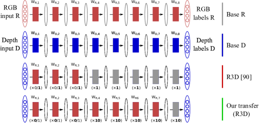
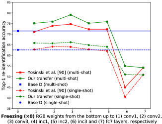
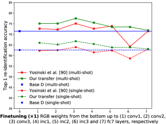
ii) We tackle the data scarcity problem in depth-based person re-identification by leveraging the large amount of RGB data to obtain stronger frame-level features. Our split-rate RGB-to-depth transfer scheme is drawn in Fig. 4. We show in Fig. 5 that our method outperforms a popular fine-tuning method by more effectively utilizing pre-trained models from RGB data.
iii) Extensive experiments in Sec. 3.5 not only show the superiority of our method compared to the state of the art in depth-based person re-identification from video, but also tackle a challenging application scenario where the persons wear clothes that were unseen during training. In Table 7 we demonstrate the robustness of our method compared to its RGB-based counterpart and the mutual gains when jointly using the person’s head information.

2 Our Method

2.1 Input Representation

The input for our system is raw depth measurements from the Kinect V$2$ [68]. The input data are depth images ${\bf D}\in\mathbb{Z}^{512\times 424}$, where each pixel $D[i,j],i\in[1,512],j\in[1,424]$, contains the Cartesian distance, in millimeters, from the image plane to the nearest object at the particular coordinate $(i,j)$. In “default range” setting, the intervals $[0,0.4m)$ and $(8.0m,\infty)$ are classified as unknown measurements, $[0.4,0.8)[m]$ as “too near”, $(4.0,8.0][m]$ as “too far” and $[0.8,4.0][m]$ as “normal” values. When skeleton tracking is effective, the body index ${\bf B}\in\mathbb{Z}^{512\times 424}$ is provided by the Kinect SDK, where $0$ corresponds to background and a positive integer $i$ for each pixel belonging to the person $i$.

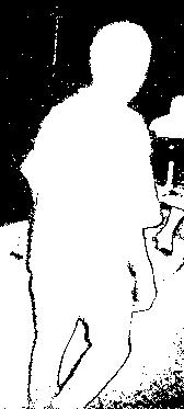
After extracting the person region ${\bf D_{p}}\subset{\bf D}$, the measurements within the “normal” region are normalized in the range $[1,256]$, while the values from “too far” and “unknown” range are set as $256$, and values within the “too near” range as $1$. In practice, in order to avoid a concentration of the values near $256$, whereas other values, say on the floor in front of the subject, span the remaining range, we introduce an offset $t_{o}=56$ and normalize in $[1,256-t_{o}]$. This results in the “grayscale” person representation ${\bf D_{p}^{g}}$. When the body index is available, we deploy ${\bf B_{p}}\subset{\bf B}$ as mask on the depth region ${\bf D_{p}}$ in order to achieve background subtraction before applying range normalization (see Fig. 2).

            ⇨

Figure 2: The cropped color image (left), the grayscale depth representation ${\bf D_{p}^{g}}$ (center) and the result after background subtraction (right) using the body index information ${\bf B_{p}}$ from skeleton tracking.

2.2 Model Structure

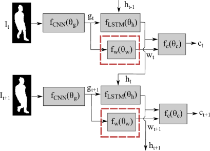
The problem is formulated as sequential decision process of an agent that performs human recognition from a partially observed environment via video sequences. At each time step, the agent observes the environment via depth camera, calculates a feature vector based on a deep Convolutional Neural Network (CNN) and actively infers the importance of the current frame for the re-identification task using novel Reinforced Temporal Attention (RTA). On top of the CNN features, a Long Short-Term Memory (LSTM) unit models short-range temporal dynamics. At each time step the agent receives a reward based on the success or failure of its classification task. Its objective is to maximize the sum of rewards over time. The agent and its components are detailed next, while the training process is described in Sec. 2.3. The model is outlined in Fig. 3.

Figure 3: Our model architecture consists of a frame-level feature embedding $f_{CNN}$, which provides input to both a recurrent layer $f_{LSTM}$ and the Reinforced Temporal Attention (RTA) unit $f_{w}$ (highlighted in red). The classifier is attached to the hidden state $h_{t}$ and its video prediction is the weighted sum of single-frame predictions, where the weights $w_{t}$ for each frame $t$ are predicted by the RTA unit.

2.2.1 Agent:

Formally, the problem setup is a Partially Observable Markov Decision Process (POMDP). The true state of the environment is unknown. The agent learns a stochastic policy $\pi((w_{t},c_{t})|s_{1:t};\theta)$ with parameters $\theta=\{\theta_{g},\theta_{w},\theta_{h},\theta_{c}\}$ that, at each step $t$, maps the past history $s_{1:t}=I_{1},w_{1},c_{1},\ldots,I_{t-1},w_{t-1},c_{t-1},I_{t}$ to two distributions over discrete actions: the frame weight $w_{t}$ (sub-policy $\pi_{1}$) and the class posterior $c_{t}$ (sub-policy $\pi_{2}$). The weight $w_{t}$ is sampled stochastically from a binary distribution parameterized by the RTA unit $f_{w}(g_{t};\theta_{w})$ at time $t$: $w_{t}\sim\pi_{1}(\cdot|f_{w}(g_{t};\theta_{w}))$. The class posterior distribution is conditioned on the classifier module, which is attached to the LSTM output $h_{t}$: $c_{t}\sim\pi_{2}(\cdot|f_{c}(h_{t};\theta_{c}))$. The vector $h_{t}$ maintains an internal state of the environment as a summary of past observations. Note that, for simplicity of notation, the input image at time $t$ is denoted as $I_{t}$, but the actual input is the person region $D_{p,t}^{g}$ (see Sec. 2.1).

2.2.2 Frame-level Feature Embedding $f_{CNN}(\theta_{g})$:

Given that there is little depth data but a large amount of RGB data available for person re-identification, we would like to leverage the RGB data to train depth models for frame-level feature extraction. We discovered that the parameters at the bottom convolutional layers of a deep neural network can be directly shared between RGB and depth data (cf. Sec. 2.3) through a simple depth encoding, that is, each pixel with depth D is replicated to three channels and encoded as (D,D,D), which corresponds to the three RGB channels. This motivates us to select a pre-trained RGB model.

RGB-based person re-identification has progressed rapidly in recent years [40, 89, 1, 82, 79, 73]. The deep convolutional network introduced by Xiao et al. [82] outperformed other approaches on several public datasets. Therefore, we decide to adopt their model for frame-level feature extraction. This network is similar in nature to GoogleNet [75]; it uses batch normalization [30] and includes $3\times 3$ convolutional layers [69], followed by $6$ Inception modules [75], and $2$ fully connected layers. In order to make this network applicable to our scenario, we introduce two small modifications. First, we replace the top classification layer with a $256\times N$ fully connected layer, where $N$ is the number of subjects at the target dataset and its weights are initialized at random from a zero-mean Gaussian distribution with standard deviation $0.01$. Second, we add dropout regularization between the fully-connected layers. In Sec. 2.3 we demonstrate an effective way to transfer the model parameters from RGB to Depth.

2.2.3 Recurrent Module $f_{LSTM}(\theta_{h})$:

We use the efficient Long Short-Term Memory (LSTM) element units as described in [92], which have been shown by Donahue et al. [20] to be effective in modeling temporal dynamics for video recognition and captioning. In specific, assuming that $\sigma()$ is sigmoid, $g[t]$ is the input at time frame $t$, $h[t-1]$ is the previous output of the module and $c[t-1]$ is the previous cell, the implementation corresponds to the following updates:

$$i[t] =\sigma(W_{gi}g[t]+W_{hi}h[t-1]+b_{i})$$ (1)

$$f[t] =\sigma(W_{gf}g[t]+W_{hf}h[t-1]+b_{f})$$ (2)

$$z[t] =tanh(W_{gc}g[t]+W_{hc}h[t-1]+b_{c})$$ (3)

$$c[t] =f[t]\odot c[t-1]+i[t]\odot z[t]$$ (4)

$$o[t] =\sigma(W_{go}g[t]+W_{ho}h[t-1]+b_{o})$$ (5)

$$h[t] =o[t]\odot tanh(c[t])$$ (6)

where $W_{sq}$ is the weight matrix from source $s$ to target $q$ for each gate $q$, $b_{q}$ are the biases leading into $q$, $i[t]$ is the input gate, $f[t]$ is the forget gate, $z[t]$ is the input to the cell, $c[t]$ is the cell, $o[t]$ is the output gate, and $h[t]$ is the output of this module. Finally, $x\odot y$ denotes the element-wise product of vectors $x$ and $y$.

2.2.4 Reinforced Temporal Attention $f_{w}(\theta_{w})$:

At each time step $t$ the RTA unit infers the importance $w_{t}$ of the image frame $I_{t}$, as the latter is represented by the feature encoding $g_{t}$. This module consists of a linear layer which maps the $256\times 1$ vector $g_{t}$ to one scalar, followed by Sigmoid non-linearity which squashes real-valued inputs to a $[0,1]$ range. Next, the output $w_{t}$ is defined by a Bernoulli random variable with probability mass function:

$$f(w_{t};f_{w}(g_{t};\theta_{w}))=\begin{cases}f_{w}(g_{t};\theta_{w}),&w_{t}=1\\ 1-f_{w}(g_{t};\theta_{w}),&w_{t}=0\end{cases}$$ (7)

The Bernoulli parameter is conditioned on the Sigmoid output $f_{w}(g_{t};\theta_{w})$, shaping a Bernoulli-Sigmoid unit [80]. During training, the output $w_{t}$ is sampled stochastically to be a binary value in $\{0,1\}$. During evaluation, instead of sampling from the distribution, the output is deterministically decided to be equal to the Bernoulli parameter and, therefore, $w_{t}=f_{w}(g_{t};\theta_{w})$.

2.2.5 Classifier $f_{c}(\theta_{c})$ and Reward:

The classifier consists of a sequence of a rectified linear unit, dropout with rate $r=0.4$, a fully connected layer and Softmax. The parametric layer maps the $256\times 1$ hidden vector $h_{t}$ to the $N\times 1$ class posterior vector $c_{t}$, which has length equal to the number of classes $N$. The multi-shot prediction with RTA attention is the weighted sum of frame-level predictions $c_{t}$, as they are weighted by the normalized, RTA weights $w_{t}^{\prime}=\frac{f_{w}(g_{t};\theta_{w})}{\sum_{t=1}^{T}f_{w}(g_{t};\theta_{w})}$.

The Bernoulli-Sigmoid unit is stochastic during training and therefore we resort to the REINFORCE algorithm in order to obtain the gradient for the backward pass. We describe the details of the training process in Sec. 2.3, but here we define the required reward function. A straightforward definition is:

$$r_{t}=\mathcal{I}(arg\,max(c_{t})=g_{t})$$ (8)

where $r_{t}$ is the raw reward, $\mathcal{I}$ is the indicator function and $g_{t}$ is the ground-truth class for frame $t$. Thus, at each time step $t$, the agent receives a reward $r_{t}$, which equals to $1$ when the frame is correctly classified and $0$ otherwise.

2.3 Model Training

In our experiments we first pre-train the parameters of the frame-level feature embedding, and afterwards we attach LSTM, RTA and the new classifier in order to train the whole model (cf. Fig. 3). At the second step the weights of the embedding are frozen while the added layers are initialized at random. We adopt this modular training so that we provide both single-shot and multi-shot evaluation, but the entire architecture can well be trained end to end from scratch if processing video sequences is the sole objective. Next, we first describe our transfer learning for the frame-level embedding and following the hybrid supervised training algorithm for the recursive model with temporal attention.

2.3.1 Split-rate Transfer Learning for Feature Embedding $f_{CNN}(\theta_{g})$:

In order to leverage on vast RGB data, our approach relies on transferring parameters $\theta_{g}$ from a RGB pre-trained model for initialization. As it is unclear whether and which subset of RGB parameters is beneficial for depth embedding, we first gain insight from work by Yosinski et al. [90] in CNN feature transferability. They showed that between two almost equal-sized splits from Imagenet [66], the most effective model adaptation is to transfer and slowly fine-tune the weights of the bottom convolutional layers, while re-training the top layers. Other works that tackle model transfer from a large to a small-sized dataset (e.g. [33]) copy and slowly fine-tune the weights of the whole hierarchy except for the classifier which is re-trained using a higher learning rate.

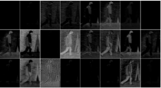
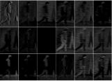
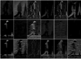
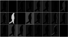
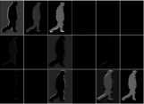
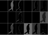
Inspired by both approaches, we investigate the model transferability between RGB and depth. Our method has three differences compared to [90]. First, we found that even though RGB and depth are quite different modalities (cf. Fig. 1), the bottom layers of the RGB models can be shared with the depth data (without fine-tuning). Second, fine-tuning parameters transferred from RGB works better than training from scratch for the top layers. Third, using slower (or zero) learning rate for the bottom layers and higher for the top layers is more effective than using uniform rate across the hierarchy. Thus, we term our method as split-rate transfer. This first and third remarks also consist key differences with [33], as firstly they fine-tune all layers and secondly they deploy higher learning rate only for the classifier. Our approach is visualized in Fig. 4 and ablation studies are shown in Sec. 3.4 and Fig. 5, which support the above-mentioned observations.

Figure 4: Our split-rate RGB-to-Depth transfer compared with Yosinski et al. [90]. At the top, the two models are trained from scratch with RGB and Depth data. Next we show the “R3D” instances (i.e. the bottom $3$ layers’ weights from RGB remain frozen or slowly changing) for both methods, following the notation of [90]. The color of each layer refers to the initialization and the number below is the relative learning rate (the best performing one in bold). The key differences are summarized in the text.

2.3.2 Hybrid Learning for CNN-LSTM and Reinforced Temporal Attention:

The parameters $\{\theta_{g},\theta_{h},\theta_{c}\}$ of CNN-LSTM are learned by minimizing the classification loss that is attached on the LSTM unit via backpropagation backward through the whole network. We minimize the cross-entropy loss as customary in recognition tasks, such as face identification [74]. Thus, the objective is to maximize the conditional probability of the true label given the observations, i.e. we maximize $\log\pi_{2}(c_{t}^{*}|s_{1:t};\theta_{g},\theta_{h},\theta_{c})$, where $c_{t}^{*}$ is the true class at step $t$.

The parameters $\{\theta_{g},\theta_{w}\}$ of CNN and RTA are learned so that the agent maximizes its total reward $R=\sum_{t=1}^{T}r_{t}$, where $r_{t}$ has defined in Eq. 8. This involves calculating the expectation $J(\theta_{g},\theta_{w})=\mathbb{E}_{p(s_{1:T};\theta_{g},\theta_{w})}[R]$ over the distribution of all possible sequences $p(s_{1:T};\theta_{g},\theta_{w})$, which is intractable. Thus, a sample approximation, known as the REINFORCE rule [80], can be applied on the Bernoulli-Sigmoid unit [44, 36], which models the sub-policy $\pi_{1}(w_{t}|f_{w}(g_{t};\theta_{w}))$. Given probability mass function $\log\pi_{1}(w_{t};p_{t})=w_{t}\log p_{t}+(1-w_{t})\log(1-p_{t})$ with Bernoulli parameter $p_{t}=f_{w}(g_{t};\theta_{w})$, the gradient approximation is:

$$\nabla_{\theta_{g},\theta_{w}}J =\sum_{t=1}^{T}\mathop{\mathbb{E}}\nolimits_{p(s_{1:T};\theta_{g},\theta_{w})}[\nabla_{\theta_{g},\theta_{w}}\log\pi_{1}(w_{t}|s_{1:t};\theta_{g},\theta_{w})(R_{t}-b_{t})]$$ (9)

$$\approx\frac{1}{M}\sum_{i=1}^{M}\sum_{t=1}^{T}\frac{w_{t}^{i}-p_{t}^{i}}{p_{t}^{i}(1-p_{t}^{i})}(R_{t}^{i}-b_{t})$$ (10)

where sequences $i$, $i\in\{1,\ldots,M\}$, are obtained while running the agent for $M$ episodes and $R_{t}^{i}=\sum_{\tau=1}^{t}r_{\tau}^{i}$ is the cumulative reward at episode $i$ acquired after collecting the sample $w_{t}^{i}$. The gradient estimate is biased by a baseline reward $b_{t}$ in order to achieve lower variance. Similarly to [56, 26], we set $b_{t}=\mathbb{E}_{\pi}[R_{t}]$, as the mean square error between $R_{t}^{i}$ and $b_{t}$ is also minimized by backpropagation.

At each step $t$, the agent makes a prediction $w_{t}$ and the reward signal $R_{t}^{i}$ evaluates the effectiveness of the agent for the classification task. The REINFORCE update increases the log-probability of an action that results in higher than the expected accumulated reward (i.e. by increasing the Bernoulli parameter $f_{w}(g_{t};\theta_{w})$). Otherwise, the log-probability decreases for sequence of frames that lead to low reward. All in all, the agent jointly optimizes the accumulated reward and the classification loss, which constitute a hybrid supervised objective.

3 Experiments

3.1 Depth-based Datasets

DPI-T (Depth-based Person Identification from Top).

Being recently introduced by Haque et al. [26], it contains $12$ persons appearing in a total of $25$ sequences across many days and wearing $5$ different sets of clothes on average. Unlike most publicly available datasets, the subjects appear from the top, which is a common scenario in automated video surveillance. The individuals are captured in daily life situations where they hold objects such as handbags, laptops and coffee.

BIWI.

In order to explore sequences with varying human pose and scale, we use BIWI [58], where $50$ individuals appear in a living room. $28$ of them are re-recorded in a different room with new clothes and walking patterns. We use the full training set, while for testing we use the Walking set. From both sets we remove the frames with no person or a person heavily occluded from the image boundaries or too far from the sensor, as they provide no skeleton information.

IIT PAVIS.

To evaluate our method when shorter video sequences are available, we use IIT PAVIS [6]. This dataset includes $79$ persons that are recorded in 5-frame walking sequences twice. We use Walking1 and Walking2 sequences as the training and testing set, respectively.

TUM-GAID.

To evaluate on a large pool of identities, we use the TUM-GAID database [28], which contains RGB and depth video for $305$ people in three variations. A subset of $32$ people is recorded a second time after three months with different clothes, which makes it ideal for our application scenario in Sec. 3.6. In our experiments we use the “normal” sequences (n) from each recording.

3.2 Evaluation Metrics

Top-k accuracy equals the percentage of test images or sequences for which the ground-truth label is contained within the first $k$ model predictions. Plotting the top-k accuracy as a function of $k$ gives the Cumulative Matching Curve (CMC). Integrating the area under the CMC curve and normalizing over the number of IDs produces the normalized Area Under the Curve (nAUC).

In single-shot mode the model consists only of the $f_{CNN}$ branch with an attached classifier (see Fig. 3). In multi-shot mode, where the model processes sequences, we evaluate our CNN-LSTM model with (or without) RTA attention.

3.3 Experimental Setting

The feature embedding $f_{CNN}$ is trained in Caffe [31]. Consistent with [82], the input depth images are resized to be $144\times 56$. SGD mini-batches of $50$ images are used for training and testing. Momentum $\mu=0.5$ yielded more stable training. The momentum effectively multiplies the size of the updates by a factor of $\frac{1}{1-\mu}$ after several iterations, so lower values result in smaller updates. The weight decay is set to $2*10^{-4}$, as it is common in Inception architecture [75]. We deploy modest base learning rate $\gamma_{0}=3\times 10^{-4}$. The learning rate is reduced by a factor of $10$ throughout training every time the loss reaches a “plateau”.

The whole model with the LSTM and RTA layers in Fig. 3 is implemented in Torch/Lua [18]. We implemented customized Caffe-to-Torch conversion scripts for the pre-trained embedding, as the architecture is not standard. For end-to-end training, we use momentum $\mu=0.9$, batch size $50$ and learning rate that linearly decreases from $0.01$ to $0.0001$ in $200$ epochs up to $250$ epochs maximum duration. The LSTM history consists of $\rho=3$ frames.

Figure 5: Comparison of our RGB-to-Depth transfer with Yosinski et al. [90] in terms of top-1 accuracy on DPI-T. In this ablation study the x axis represents the number of layers whose weights are frozen (left) or fine-tuned (right) starting from the bottom.

3.4 Evaluation of the Split-Rate RGB-to-Depth Transfer

In Fig. 5 we show results of our split-rate RGB-to-Depth transfer (which is described in Sec. 2.3) compared to [90]. We show the top-1 re-identification accuracy on DPI-T when the bottom CNN layers are frozen (left) and slowly fine-tuned (right). The top layers are transferred from RGB and rapidly fine-tuned in our approach, while they were re-trained in [90]. Given that the CNN architecture has $7$ main layers before the classifier, the $x$ axis is the number of layers that are frozen or fine-tuned counting from the bottom.

Evidently, transferring and freezing the three bottom layers, while rapidly fine-tuning the subsequent “inception” and fully-connected layers, brings in the best performance on DPI-T. Attempting to freeze too many layers leads to performance drop for both approaches, which can been attributed to feature specificity. Slowly fine-tuning the bottom layers helps to alleviate fragile co-adaptation, as it was pointed out by Yosinski et al. [90], and improves generalization, especially while moving towards the right of the x axis. Overall, our approach is more accurate in our setting across the x axis for both treatments.

3.5 Evaluation of the End-to-End Framework

Table 1: Single-shot and multi-shot person re-identification performance on the test set of DPI-T, BIWI and IIT PAVIS. Dashes indicate that no published result is available

Mode	Method	Top-1 Accuracy ($\%$)
		DPI-T	BIWI	IIT PAVIS
	Random	8.3	2.0	1.3
Single-shot	Skeleton (NN) [58]	–	21.1	28.6
	Skeleton (SVM) [59]	–	13.8	35.7
	3D RAM [26]	47.5	30.1	41.3
	Our method (CNN)	66.8	25.4	43.0
Multi-shot	Skeleton (NN) [58]	–	39.3	–
	Skeleton (SVM) [59]	–	17.9	–
	Energy Volume [70]	14.2	25.7	18.9
	3D CNN+Avg Pooling [8]	28.4	27.8	27.5
	4D RAM [26]	55.6	45.3	43.0
	Our method (CNN-LSTM+Avg Pooling )	75.5	45.7	50.1
	Our method with attention from [88]	75.9	46.4	50.6
	Our method with RTA attention	76.3	50.0	52.4

In Table 1 we compare our framework with depth-based baseline algorithms. First, we show the performance of guessing uniformly at random. Next, we report results from [6, 59], who use hand-crafted features based on biometrics, such as distances between skeleton joints. A 3D CNN with average pooling over time [8] and the gait energy volume [70] are evaluated in multi-shot mode. Finally, we provide the comparisons with 3D and 4D RAM models [26].

In order to evaluate our model in multi-shot mode without temporal attention, we simply average the output of the classifier attached on the CNN-LSTM output across the sequence (cf. Fig. 3). In the last two rows we show results that leverage temporal attention. We compare our RTA attention with the soft attention in [88], which is a function of both the hidden state $h_{t}$ and the embedding $g_{t}$, whose projections are added and passed through a $tanh$ non-linearity.

We observe that methods that learn end-to-end re-identification features perform significantly better than the ones that rely on hand-crafted biometrics on all datasets. Our algorithm is the top performer in multi-shot mode, as our RTA unit effectively learns to re-weight the most effective frames based on classification-specific reward. The split-rate RGB-to-Depth transfer enables our method to leverage on RGB data effectively and provides discriminative depth-based ReID features. This is especially reflected by the single-shot accuracy on DPI-T, where we report $19.3\%$ better top-1 accuracy compared to 3D RAM. However, it is worth noting that 3D RAM performs better on BIWI. Our conjecture is that the spatial attention mechanism is important in datasets with significant variation in human pose and partial body occlusions. On the other hand, the spatial attention is evidently less critical on DPI-T, which contains views from the top and the visible region is mostly uniform across frames.

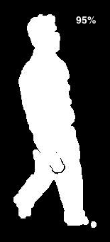
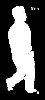
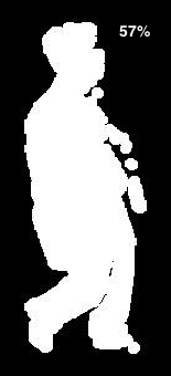
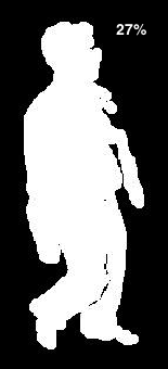
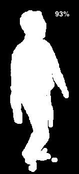
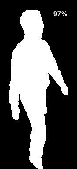
Next in Fig. 6 we show a testing sequence with the predicted Bernoulli parameter $f_{w}(g_{t};\theta_{w})$ printed. After inspecting the Bernoulli parameter value on testing sequences, we observe large variations even among neighboring frames. Smaller values are typically associated with noisy frames, or frames with unusual pose (e.g. person turning) and partial occlusions.

              

Figure 6: Example sequence with the predicted Bernoulli parameter printed.

Figure 7: Cumulative Matching Curves (CMC) on TUM-GAID for the scenario that the individuals wear clothes which are not provided during training.

Table 2: Top-1 re-identification accuracy (top-1, $\%$) and normalized Area Under the Curve (nAUC, $\%$) on TUM-GAID in new-clothes scenario with single-shot (ss) and multi-shot (ms) evaluation

Modality	top-$1$	nAUC
Body RGB (ss) [82]	41.8	74.3
Body Depth (ss)	48.0	85.0
Body Depth & RGB (ss)	48.6	81.9
Head RGB (ss)	59.4	79.5
Body Depth & Head RGB (ss)	65.4	85.2
Body RGB (ms: LSTM & RTA)	50.0	79.9
Body Depth (ms: LSTM)	56.3	87.7
Body Depth (ms: LSTM & RTA)	59.4	89.6
Head RGB (ms: LSTM & RTA)	65.6	81.0
Body Depth & Head RGB (ms: LSTM & RTA)	75.0	88.1

3.6 Application in Scenario with Unseen Clothes

Towards tackling our key motivation, we compare our system compared to a state-of-the-art RGB method in scenario where the individuals change clothes between the recordings for training and test set. We use the TUM-GAID database at which $305$ persons appear in sequences $n01$–$n06$ from session $1$, and $32$ among them appear with new clothes in sequences $n07$–$n12$ from session $2$.

Following the official protocol, we use the Training IDs to perform RGB-to-Depth transfer for our CNN embedding. We use sequences $n01$–$n04$, $n07$–$n10$ for training, and sequences $n05$–$n06$ and $n11$–$n12$ for validation. Next, we deploy the Testing IDs and use sequences $n01$–$n04$ for training, $n05$–$n06$ for validation and $n11$–$n12$ for testing. Thus, our framework has no access to data from the session $2$ during training. However, we make the assumption that the $32$ subjects that participate in the second recording are known for all competing methods.

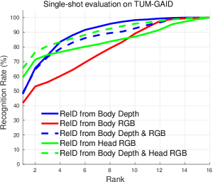
In Table 7 we show that re-identification from body depth is more robust than from body RGB [82], presenting $6.2\%$ higher top-1 accuracy and $10.7\%$ larger nAUC in single-shot mode. Next, we explore the benefit of using head information, which is less sensitive than clothes to day-by-day changes. To that end, we transfer the RGB-based pre-trained model from [82] and fine-tune on the upper body part, which we call “Head RGB”. This results in increased accuracy, individually and jointly with body depth. Finally, we show the mutual benefits in multi-shot performance for both body depth, head RGB and their linear combination in class posterior. In Fig. 7 we visualize the CMC curves for single-shot setting. We observe that ReID from body depth scales better than its counterparts, which is validated by the nAUC scores.

4 Conclusion

In the paper, we present a novel approach for depth-based person re-identification. To address the data scarcity problem, we propose split-rate RGB-depth transfer to effectively leverage pre-trained models from large RGB data and learn strong frame-level features. To enhance re-identification from video sequences, we propose the Reinforced Temporal Attention unit, which lies on top of the frame-level features and is not dependent on the network architecture. Extensive experiments show that our approach outperforms the state of the art in depth-based person re-identification, and it is more effective than its RGB-based counterpart in a scenario where the persons change clothes.

Acknowledgments:

This work was supported in part by ARO W911NF-15-1- 0564/66731-CS, ONR N00014-13-1-034, and AFOSR FA9550-15-1-0229.

References

- [1] Ahmed, E., Jones, M., Marks, T.K.: An improved deep learning architecture for person re-identification. In: CVPR (2015)
- [2] Albiol, A., Oliver, J., Mossi, J.: Who is who at different cameras: people re-identification using depth cameras. IET Computer Vision (2012)
- [3] Andersson, V., Dutra, R., Araújo, R.: Anthropometric and human gait identification using skeleton data from kinect sensor. In: ACM Symposium on Applied Computing (2014)
- [4] Bai, S., Bai, X., Tian, Q.: Scalable person re-identification on supervised smoothed manifold. In: CVPR (2017)
- [5] Bak, S., Carr, P.: One-shot metric learning for person re-identification. In: CVPR (2017)
- [6] Barbosa, I., Cristani, M., Del Bue, A., Bazzani, L., Murino, V.: Re-identification with RGB-D sensors. In: ECCV Workshops (2012)
- [7] Bedagkar-Gala, A., Shah, S.K.: A survey of approaches and trends in person re-identification. Image and Vision Computing (2014)
- [8] Boureau, Y.L., Ponce, J., LeCun, Y.: A theoretical analysis of feature pooling in visual recognition. In: ICML (2010)
- [9] Castro, F.M., Marín-Jiménez, M.J., Guil, N., de la Blanca, N.P.: Automatic learning of gait signatures for people identification. In: International Work-Conference on Artificial Neural Networks (2017)
- [10] Castro, F.M., Marín-Jimenez, M.J., Medina-Carnicer, R.: Pyramidal fisher motion for multiview gait recognition. In: ICPR (2014)
- [11] Chan, W., Jaitly, N., Le, Q.V., Vinyals, O.: Listen, attend and spell. ICASSP (2016)
- [12] Chen, D., Yuan, Z., Chen, B., Zheng, N.: Similarity learning with spatial constraints for person re-identification. In: CVPR (2016)
- [13] Chen, J., Wang, Y., Qin, J., Liu, L., Shao, L.: Fast person re-identification via cross-camera semantic binary transformation. In: CVPR (2017)
- [14] Chen, L.F., Liao, H.Y.M., Ko, M.T., Lin, J.C., Yu, G.J.: A new lda-based face recognition system which can solve the small sample size problem. Pattern Recognition (2000)
- [15] Chen, W., Chen, X., Zhang, J., Huang, K.: Beyond triplet loss: A deep quadruplet network for person re-identification. In: CVPR (2017)
- [16] Cho, Y.J., Yoon, K.J.: Improving person re-identification via pose-aware multi-shot matching. In: CVPR (2016)
- [17] Chung, D., Tahboub, K., Delp, E.J.: A two stream siamese convolutional neural network for person re-identification. In: ICCV (2017)
- [18] Collobert, R., Kavukcuoglu, K., Farabet, C.: Torch7: A matlab-like environment for machine learning. In: BigLearn, NIPS Workshop (2011)
- [19] Ding, S., Lin, L., Wang, G., Chao, H.: Deep feature learning with relative distance comparison for person re-identification. Pattern Recognition (2015)
- [20] Donahue, J., Anne Hendricks, L., Guadarrama, S., Rohrbach, M., Venugopalan, S., Saenko, K., Darrell, T.: Long-term recurrent convolutional networks for visual recognition and description. In: CVPR (2015)
- [21] Dubois, A., Charpillet, F.: A gait analysis method based on a depth camera for fall prevention. In: IEEE Engineering in Medicine and Biology Society (2014)
- [22] Farenzena, M., Bazzani, L., Perina, A., Murino, V., Cristani, M.: Person re-identification by symmetry-driven accumulation of local features. In: CVPR (2010)
- [23] Gong, S., Cristani, M., Yan, S., Loy, C.C.: Person re-identification (2014)
- [24] Gray, D., Tao, H.: Viewpoint invariant pedestrian recognition with an ensemble of localized features. ECCV (2008)
- [25] Gupta, S., Girshick, R., Arbeláez, P., Malik, J.: Learning rich features from rgb-d images for object detection and segmentation. In: ECCV (2014)
- [26] Haque, A., Alahi, A., Fei-Fei, L.: Recurrent attention models for depth-based person identification. In: CVPR (2016)
- [27] Hinton, G.E., Srivastava, N., Krizhevsky, A., Sutskever, I., Salakhutdinov, R.R.: Improving neural networks by preventing co-adaptation of feature detectors. Preprint arXiv:1207.0580 (2012)
- [28] Hofmann, M., Geiger, J., Bachmann, S., Schuller, B., Rigoll, G.: The TUM Gait from Audio, Image and Depth database: Multimodal recognition of subjects and traits. Journal of Visual Communication and Image Representation (2014)
- [29] Ioannidis, D., Tzovaras, D., Damousis, I.G., Argyropoulos, S., Moustakas, K.: Gait recognition using compact feature extraction transforms and depth information. IEEE Transactions on Information Forensics and Security (2007)
- [30] Ioffe, S., Szegedy, C.: Batch normalization: Accelerating deep network training by reducing internal covariate shift. ICML (2015)
- [31] Jia, Y., Shelhamer, E., Donahue, J., Karayev, S., Long, J., Girshick, R., Guadarrama, S., Darrell, T.: Caffe: Convolutional architecture for fast feature embedding. In: Proceedings of the ACM international conference on Multimedia (2014)
- [32] Kale, A., Cuntoor, N., Yegnanarayana, B., Rajagopalan, A., Chellappa, R.: Gait analysis for human identification. In: International Conference on Audio-and Video-Based Biometric Person Authentication (2003)
- [33] Karayev, S., Trentacoste, M., Han, H., Agarwala, A., Darrell, T., Hertzmann, A., Winnemoeller, H.: Recognizing image style (2014)
- [34] Kodirov, E., Xiang, T., Fu, Z., Gong, S.: Person re-identification by unsupervised graph learning. In: ECCV (2016)
- [35] Koestinger, M., Hirzer, M., Wohlhart, P., Roth, P.M., Bischof, H.: Large scale metric learning from equivalence constraints. In: CVPR (2012)
- [36] Kontoravdis, D., Likas, A., Stafylopatis, A.: Enhancing stochasticity in reinforcement learning schemes: Application to the exploration of binary domains. Journal of Intelligent Systems (1995)
- [37] Krizhevsky, A., Sutskever, I., Hinton, G.E.: Imagenet classification with deep convolutional neural networks. In: NIPS (2012)
- [38] Kviatkovsky, I., Adam, A., Rivlin, E.: Color invariants for person re-identification. IEEE Transactions on Pattern Analysis and Machine Intelligence (2013)
- [39] Li, D., Chen, X., Zhang, Z., Huang, K.: Learning deep context-aware features over body and latent parts for person re-identification. In: CVPR (2017)
- [40] Li, W., Zhao, R., Xiao, T., Wang, X.: DeepReID: deep filter pairing neural network for person re-identification. In: CVPR (2014)
- [41] Li, Y., Lin, G., Zhuang, B., Liu, L., Shen, C., van den Hengel, A.: Sequential person recognition in photo albums with a recurrent network. In: CVPR (2017)
- [42] Li, Z., Chang, S., Liang, F., Huang, T.S., Cao, L., Smith, J.R.: Learning locally-adaptive decision functions for person verification. In: CVPR (2013)
- [43] Liao, S., Hu, Y., Zhu, X., Li, S.Z.: Person re-identification by local maximal occurrence representation and metric learning. In: CVPR (2015)
- [44] Likas, A.: A reinforcement learning approach to online clustering. Neural Computation (1999)
- [45] Lin, J., Ren, L., Lu, J., Feng, J., Zhou, J.: Consistent-aware deep learning for person re-identification in a camera network. In: CVPR (2017)
- [46] Lisanti, G., Masi, I., Bagdanov, A.D., Del Bimbo, A.: Person re-identification by iterative re-weighted sparse ranking. IEEE Transactions on Pattern Analysis and Machine Intelligence (2015)
- [47] Lisanti, G., Masi, I., Del Bimbo, A.: Matching people across camera views using kernel canonical correlation analysis. In: Proceedings of the International Conference on Distributed Smart Cameras. ACM (2014)
- [48] Liu, Z., Wang, D., Lu, H.: Stepwise metric promotion for unsupervised video person re-identification. In: ICCV (2017)
- [49] Luong, M.T., Pham, H., Manning, C.D.: Effective approaches to attention-based neural machine translation. EMNLP (2015)
- [50] Ma, B., Su, Y., Jurie, F.: Local descriptors encoded by fisher vectors for person re-identification. In: ECCV Workshops (2012)
- [51] Ma, L., Yang, X., Tao, D.: Person re-identification over camera networks using multi-task distance metric learning. IEEE Transactions on Image Processing (2014)
- [52] Mansur, A., Makihara, Y., Aqmar, R., Yagi, Y.: Gait recognition under speed transition. In: CVPR (2014)
- [53] Martinel, N., Das, A., Micheloni, C., Roy-Chowdhury, A.K.: Temporal model adaptation for person re-identification. In: ECCV (2016)
- [54] McLaughlin, N., Martinez del Rincon, J., Miller, P.: Recurrent convolutional network for video-based person re-identification. In: CVPR (2016)
- [55] Mignon, A., Jurie, F.: PCCA: A new approach for distance learning from sparse pairwise constraints. In: CVPR (2012)
- [56] Mnih, V., Heess, N., Graves, A., et al.: Recurrent models of visual attention. In: NIPS (2014)
- [57] Mogelmose, A., Moeslund, T.B., Nasrollahi, K.: Multimodal person re-identification using rgb-d sensors and a transient identification database. In: IEEE International Workshop on Biometrics and Forensics (2013)
- [58] Munaro, M., Basso, A., Fossati, A., Van Gool, L., Menegatti, E.: 3d reconstruction of freely moving persons for re-identification with a depth sensor. In: ICRA (2014)
- [59] Munaro, M., Fossati, A., Basso, A., Menegatti, E., Van Gool, L.: One-shot person re-identification with a consumer depth camera. In: Person Re-Identification (2014)
- [60] Munsell, B., Temlyakov, A., Qu, C., Wang, S.: Person identification using full-body motion and anthropometric biometrics from kinect videos. In: ECCV Workshops (2012)
- [61] Paisitkriangkrai, S., Shen, C., van den Hengel, A.: Learning to rank in person re-identification with metric ensembles. In: CVPR (2015)
- [62] Pathak, D., Girshick, R.B., Dollár, P., Darrell, T., Hariharan, B.: Learning features by watching objects move. In: CVPR (2017)
- [63] Pedagadi, S., Orwell, J., Velastin, S., Boghossian, B.: Local fisher discriminant analysis for pedestrian re-identification. In: CVPR (2013)
- [64] Prosser, B., Zheng, W.S., Gong, S., Xiang, T., Mary, Q.: Person re-identification by support vector ranking. In: BMVC (2010)
- [65] Qian, X., Fu, Y., Jiang, Y.G., Xiang, T., Xue, X.: Multi-scale deep learning architectures for person re-identification. In: ICCV (2017)
- [66] Russakovsky, O., Deng, J., Su, H., Krause, J., Satheesh, S., Ma, S., Huang, Z., Karpathy, A., Khosla, A., Bernstein, M., et al.: Imagenet large scale visual recognition challenge. International Journal of Computer Vision (2015)
- [67] Shi, H., Yang, Y., Zhu, X., Liao, S., Lei, Z., Zheng, W., Li, S.Z.: Embedding deep metric for person re-identification: A study against large variations. In: ECCV (2016)
- [68] Shotton, J., Sharp, T., Kipman, A., Fitzgibbon, A., Finocchio, M., Blake, A., Cook, M., Moore, R.: Real-time human pose recognition in parts from single depth images. Communications of the ACM (2013)
- [69] Simonyan, K., Zisserman, A.: Very deep convolutional networks for large-scale image recognition. ICLR (2015)
- [70] Sivapalan, S., Chen, D., Denman, S., Sridharan, S., Fookes, C.: Gait energy volumes and frontal gait recognition using depth images. In: International Joint Conference on Biometrics (2011)
- [71] Song, X., Herranz, L., Jiang, S.: Depth cnns for rgb-d scene recognition: Learning from scratch better than transferring from rgb-cnns. In: AAAI (2017)
- [72] Su, C., Li, J., Zhang, S., Xing, J., Gao, W., Tian, Q.: Pose-driven deep convolutional model for person re-identification. In: ICCV (2017)
- [73] Su, C., Zhang, S., Xing, J., Gao, W., Tian, Q.: Deep attributes driven multi-camera person re-identification. In: ECCV (2016)
- [74] Sun, Y., Wang, X., Tang, X.: Deep learning face representation from predicting 10,000 classes. In: CVPR (2014)
- [75] Szegedy, C., Liu, W., Jia, Y., Sermanet, P., Reed, S., Anguelov, D., Erhan, D., Vanhoucke, V., Rabinovich, A.: Going deeper with convolutions. In: CVPR (2015)
- [76] Tang, S., Andriluka, M., Andres, B., Schiele, B.: Multiple people tracking by lifted multicut and person re-identification. In: CVPR (2017)
- [77] Tao, D., Jin, L., Wang, Y., Yuan, Y., Li, X.: Person re-identification by regularized smoothing kiss metric learning. IEEE Transactions on Circuits and Systems for Video Technology (2013)
- [78] Vezzani, R., Baltieri, D., Cucchiara, R.: People re-identification in surveillance and forensics: A survey. ACM Computing Surveys (2013)
- [79] Wang, F., Zuo, W., Lin, L., Zhang, D., Zhang, L.: Joint learning of single-image and cross-image representations for person re-identification. In: CVPR (2016)
- [80] Williams, R.J.: Simple statistical gradient-following algorithms for connectionist reinforcement learning. Machine Learning (1992)
- [81] Wu, A., Zheng, W.S., Yu, H.X., Gong, S., Lai, J.: RGB-infrared cross-modality person re-identification. In: ICCV (2017)
- [82] Xiao, T., Li, H., Ouyang, W., Wang, X.: Learning deep feature representations with domain guided dropout for person re-identification. In: CVPR (2016)
- [83] Xiao, T., Li, S., Wang, B., Lin, L., Wang, X.: Joint detection and identification feature learning for person search. In: CVPR (2017)
- [84] Xiong, F., Gou, M., Camps, O., Sznaier, M.: Person re-identification using kernel-based metric learning methods. In: ECCV (2014)
- [85] Xu, S., Cheng, Y., Gu, K., Yang, Y., Chang, S., Zhou, P.: Jointly attentive spatial-temporal pooling networks for video-based person re-identification. In: ICCV (2017)
- [86] Yan, Y., Ni, B., Song, Z., Ma, C., Yan, Y., Yang, X.: Person re-identification via recurrent feature aggregation. In: ECCV (2016)
- [87] Yang, Y., Yang, J., Yan, J., Liao, S., Yi, D., Li, S.Z.: Salient color names for person re-identification. In: ECCV (2014)
- [88] Yao, L., Torabi, A., Cho, K., Ballas, N., Pal, C., Larochelle, H., Courville, A.: Describing videos by exploiting temporal structure. In: ICCV (2015)
- [89] Yi, D., Lei, Z., Liao, S., Li, S.Z.: Deep metric learning for person re-identification. In: ICPR (2014)
- [90] Yosinski, J., Clune, J., Bengio, Y., Lipson, H.: How transferable are features in deep neural networks? In: NIPS (2014)
- [91] Yu, H.X., Wu, A., Zheng, W.S.: Cross-view asymmetric metric learning for unsupervised person re-identification. In: ICCV (2017)
- [92] Zaremba, W., Sutskever, I.: Learning to execute. Preprint arXiv:1410.4615 (2014)
- [93] Zeng, W., Wang, C., Yang, F.: Silhouette-based gait recognition via deterministic learning. Pattern Recognition (2014)
- [94] Zhang, L., Xiang, T., Gong, S.: Learning a discriminative null space for person re-identification. In: CVPR (2016)
- [95] Zhao, G., Liu, G., Li, H., Pietikainen, M.: 3d gait recognition using multiple cameras. In: Automatic Face and Gesture Recognition (2006)
- [96] Zhao, H., Tian, M., Sun, S., Shao, J., Yan, J., Yi, S., Wang, X., Tang, X.: Spindle net: Person re-identification with human body region guided feature decomposition and fusion. In: CVPR (2017)
- [97] Zhao, L., Li, X., Zhuang, Y., Wang, J.: Deeply-learned part-aligned representations for person re-identification. In: ICCV (2017)
- [98] Zhao, R., Ouyang, W., Wang, X.: Person re-identification by salience matching. In: ICCV (2013)
- [99] Zhao, R., Ouyang, W., Wang, X.: Unsupervised salience learning for person re-identification. In: CVPR (2013)
- [100] Zhao, R., Ouyang, W., Wang, X.: Learning mid-level filters for person re-identification. In: CVPR (2014)
- [101] Zheng, K., Fan, X., Lin, Y., Guo, H., Yu, H., Guo, D., Wang, S.: Learning view-invariant features for person identification in temporally synchronized videos taken by wearable cameras. In: ICCV (2017)
- [102] Zheng, L., Bie, Z., Sun, Y., Wang, J., Su, C., Wang, S., Tian, Q.: Mars: A video benchmark for large-scale person re-identification. In: ECCV (2016)
- [103] Zheng, L., Shen, L., Tian, L., Wang, S., Wang, J., Tian, Q.: Scalable person re-identification: A benchmark. In: ICCV (2015)
- [104] Zheng, L., Zhang, H., Sun, S., Chandraker, M., Yang, Y., Tian, Q.: Person re-identification in the wild. In: CVPR (2017)
- [105] Zheng, W.S., Gong, S., Xiang, T.: Re-identification by relative distance comparison. IEEE Transactions on Pattern Analysis and Machine Intelligence (2013)
- [106] Zheng, Z., Zheng, L., Yang, Y.: Unlabeled samples generated by gan improve the person re-identification baseline in vitro. In: ICCV (2017)
- [107] Zhong, Z., Zheng, L., Cao, D., Li, S.: Re-ranking person re-identification with k-reciprocal encoding. In: CVPR (2017)
- [108] Zhou, J., Yu, P., Tang, W., Wu, Y.: Efficient online local metric adaptation via negative samples for person re-identification. In: ICCV (2017)
- [109] Zhou, S., Wang, J., Wang, J., Gong, Y., Zheng, N.: Point to set similarity based deep feature learning for person re-identification. In: CVPR (2017)
- [110] Zhou, Z., Huang, Y., Wang, W., Wang, L., Tan, T.: See the forest for the trees: Joint spatial and temporal recurrent neural networks for video-based person re-identification. In: CVPR (2017)