Inexpensive Cost-Optimized Measurement Proposal
for Sequential Model-Based Diagnosis

Abstract

In this work we present strategies for (optimal) measurement selection in model-based sequential diagnosis. In particular, assuming a set of leading diagnoses being given, we show how queries (sets of measurements) can be computed and optimized along two dimensions: expected number of queries and cost per query. By means of a suitable decoupling of two optimizations and a clever search space reduction the computations are done without any inference engine calls. For the full search space, we give a method requiring only a polynomial number of inferences and guaranteeing query properties existing methods cannot provide. Evaluation results using real-world problems indicate that the new method computes (virtually) optimal queries instantly independently of the size and complexity of the considered diagnosis problems.

1 Introduction

Model-based diagnosis (MBD) is a widely applied approach to finding explanations, called diagnoses, for unexpected behavior of observed systems including hardware, software, knowledge bases, discrete event systems, feature models, user interfaces, etc. Reiter (1987); Dressler and Struss (1996); Mateis et al. (2000); Pencolé and Cordier (2005); Kalyanpur et al. (2007); Felfernig et al. (2009); White et al. (2010). In case the provided observations are insufficient for successful fault localization, sequential diagnosis (SQD) methods collect additional information by generating a sequence of queries de Kleer and Williams (1987); Pietersma et al. (2005); Feldman et al. (2010); Siddiqi and Huang (2011); Shchekotykhin et al. (2012). As query answering is often costly, the goal of SQD is to minimize the diagnostic cost, like time or manpower, required to achieve a diagnostic goal, e.g. a highly probable diagnosis. To this end, the cited SQD works minimize the number of queries by a one-step lookahead measure $m$, e.g. entropy de Kleer and Williams (1987), but do not optimize the query cost, such as the time required to perform measurements Heckerman et al. (1995).

Contributions. We present a novel query optimization method that is generally applicable to any MBD problem in the sense of de Kleer and Williams (1987); Reiter (1987) and
(1) defines a query as a set of first-order sentences and thus generalizes the measurement notion of de Kleer and Williams (1987); Reiter (1987),
(2) given a set of leading diagnoses de Kleer and Williams (1989), allows the two-dimensional optimization of the next query in terms of the expected number of subsequent queries (measure $m$) and query cost (measure $c$),
(3) for an aptly refined (yet exponential) query search space, finds – without any reasoner calls – the globally optimal query wrt. measure $c$ that globally optimizes measure $m$,
(4) for the full query search space, finds – with a polynomial number of reasoner calls – the (under reasonable assumptions) globally optimal query wrt. $m$ that includes, if possible, only “cost-preferred” sentences, such as those answerable automatically using built-in sensors,
(5) guarantees the proposal of queries that discriminate between all leading diagnoses and that unambiguously identify the actual diagnosis.

The efficiency of our approach is possible by the recognition that the optimizations of $m$ and $c$ can be decoupled and by using logical monotonicity as well as the inherent (already inferred) information in the ($\subseteq$-minimal) leading diagnoses. In particular, the method is inexpensive as it (a) avoids the generation and examination of unnecessary (non-discriminating) or duplicate query candidates, (b) actuallycomputes only the single best query by its ability to estimate a query’s quality without computing it, and (c) guarantees soundness and completeness wrt. an exponential query search space independently of the properties and output of a reasoner. Modern SQD methods like de Kleer and Williams (1987) and its derivatives Feldman et al. (2010); Shchekotykhin et al. (2012); Rodler et al. (2013) do not meet all properties (a) – (c) and extensively call a reasoner for (precomputed) inferences while computing a query. Moreover, by the generality of our query notion, our method explores a more complex search space than de Kleer and Williams (1987); de Kleer and Raiman (1993), thereby guaranteeing property (5) above.

sd	$\left\{\lnot\textsc{ab}(c_{i})\rightarrow beh(c_{i})\mid c_{i}\in\textsc{comps}\right\}$
comps	$\left\{c_{1},c_{2},c_{3},c_{4},c_{5}\right\}$
normal behavior $beh(c_{i})$ of components $c_{i}\in\textsc{comps}$	$beh(c_{1}):A\rightarrow B\land L$	$beh(c_{2}):A\to F$
	$beh(c_{3}):B\lor F\to H$	$beh(c_{4}):L\to H$
	$beh(c_{5}):\lnot H\to G\land\lnot A$
$\mathit{N}$	$\mathit{n}_{1}:\left\{A\to H\right\}$	$\textsc{obs},\mathit{P}=\emptyset$

Table 1: Running Example DPI $\mathsf{Ex}$

2 Preliminaries

Model-Based Diagnosis (MBD).

In this section we recap on important MBD concepts and draw on definitions of Reiter (1987) to characterize a system and diagnoses.
Notation (*): Let $X$ be a collection of sets, then $U_{X}$ and $I_{X}$ denote the union and intersection of all elements of $X$, resp. $K\models S$ for a set $S$ is a shorthand for $K\models s$ for all $s\in S$.∎

A system consists of a set of components comps and a system description sd where $\{\lnot\textsc{ab}(c)\rightarrow beh(c)\mid c\in\textsc{comps}\}\subseteq\textsc{sd}$. The first-order sentence $beh(c)$ describes the normal behavior of $c$ and ab is a distinguished abnormality predicate. Any behavior different from $beh(c)$ implies that component $c$ is at fault, i.e. $\textsc{ab}(c)$ holds. Note, $\textsc{sd}\cup\{\lnot\textsc{ab}(c)\mid c\in\textsc{comps}\}$ is required to be consistent.

From the viewpoint of system diagnosis, evidence about the system behavior in terms of observations obs, positive ($\mathit{P}$) and negative ($\mathit{N}$) measurements Reiter (1987); de Kleer and Williams (1987); Felfernig et al. (2004) is of interest.

Definition 1 (DPI).

Let comps be a finite set of constants and sd, obs, all $\mathit{p}\in\mathit{P}$, all $\mathit{n}\in\mathit{N}$ be finite sets of consistent first-order sentences. Then $(\textsc{sd},\textsc{comps}$, $\textsc{obs},\mathit{P},\mathit{N})$ is a diagnosis problem instance (DPI).

Definition 2.

Let $(\textsc{sd},\textsc{comps},\textsc{obs},\mathit{P},\mathit{N})$ be a DPI. Then $\textsc{sd}^{*}[\Delta]:=\textsc{sd}\cup\textsc{obs}\cup U_{\mathit{P}}\cup\{\textsc{ab}(c)\mid c\in\Delta\}\cup\{\lnot\textsc{ab}(c)\mid c\in\textsc{comps}\setminus\Delta\}$ denotes the behavior description of a system $(\textsc{sd},\textsc{comps})$ given observations obs, union of positive measurements $U_{\mathit{P}}$ as well as that all components $\Delta\subseteq\textsc{comps}$ are faulty and all components in $\textsc{comps}\setminus\Delta$ are healthy.

The solutions of a DPI, i.e. the hypotheses that explain a given (faulty) system behavior, are called diagnoses:

Definition 3 (Diagnosis).

$\Delta\subseteq\textsc{comps}$ is a diagnosis for the DPI $(\textsc{sd},\textsc{comps},\textsc{obs},\mathit{P},\mathit{N})$ iff $\Delta$ is $\subseteq$-minimal such that

• $\textsc{sd}^{*}[\Delta]$ is consistent ($\Delta$ explains obs and $\mathit{P}$), and

• $\forall n\in\mathit{N}:\textsc{sd}^{*}[\Delta]\not\models n$ ($\Delta$ explains $\mathit{N}$).

We denote the set of all diagnoses for a DPI $X$ by ${\mathfrak{D}}_{X}$.

A diagnosis for a DPI exists iff $\textsc{sd}^{*}[\textsc{comps}]\not\models n$ for all $n\in N$ (Friedrich and Shchekotykhin, 2005, Prop. 1).

Example: Consider DPI $\mathsf{Ex}$ (Tab. 1). Using e.g. HS-Tree Reiter (1987) we get (denoting components $c_{i}$ by $i$) the set of all diagnoses ${\mathfrak{D}}_{\mathsf{Ex}}=\{\Delta_{1},\Delta_{2},\Delta_{3}\}=\{\{1,2,5\},\{1,3,5\}$, $\{3,4,5\}\}$. E.g. $\Delta_{2}\in{\mathfrak{D}}_{\mathsf{Ex}}$ due to Def. 3 and as $\textsc{sd}^{*}[\Delta_{2}]=[\textsc{sd}\cup\{\textsc{ab}(c_{1}),\textsc{ab}(c_{3}),\textsc{ab}(c_{5})\}\cup\{\lnot\textsc{ab}(c_{2}),\lnot\textsc{ab}(c_{4})\}]\cup\textsc{obs}\cup U_{\mathit{P}}=[\{beh(c_{2}),beh(c_{4})\}]\cup\emptyset\cup\emptyset=\{A\to F,L\to H\}\not\models$ $\{A\to H\}=n_{1}\in\mathit{N}$ and is consistent.∎

Sequential Diagnosis (SQD). Given multiple diagnoses for a DPI, SQD techniques extend the sets $P$ and $N$ by asking a user or an oracle (e.g. an automated system) to perform additional measurements in order to rule out irrelevant diagnoses. In line with the works of Settles (2012); Shchekotykhin et al. (2012); Rodler (2015) we call a proposed measurement query and define it very generally as a set of first-order sentences (this subsumes the notion of measurement e.g. in de Kleer and Williams (1987); Reiter (1987)). The task of the oracle is to assess the correctness of the sentences in the query, thereby providing the required measurements. A query $Q$ is $\mathit{true}$ ($t$) if all sentences in $Q$ are correct and $\mathit{false}$ ($f$) if at least one sentence in $Q$ is incorrect.

Usually only a small computationally feasible set of leading diagnoses ${\bf{D}}$ (e.g. minimum cardinality Feldman et al. (2010) or most probable de Kleer (1991) ones) are exploited for measurement selection de Kleer and Williams (1989).

Any sets of diagnoses and first-order sentences satisfy:

Property 1.

Let $X$ be a set of first-order sentences and ${\bf{D}}\subseteq{\mathfrak{D}}_{\mathsf{DPI}}$ for $\mathsf{DPI}=(\textsc{sd},\textsc{comps},\textsc{obs},P,N)$. Then $X$ induces a partition $\mathfrak{P}_{\bf{D}}(X):=\left\langle{\bf D}^{+}(X),{\bf D}^{-}(X),{\bf D}^{0}(X)\right\rangle$ on ${\bf{D}}$ where ${\bf D}^{+}(X):=\{\Delta\in{\bf{D}}\mid\textsc{sd}^{*}[\Delta]\models X\}$, ${\bf D}^{-}(X):=\{\Delta\in{\bf{D}}\mid\exists s\in N\cup\left\{\bot\right\}:\textsc{sd}^{*}[\Delta]\cup X\models s\}$ and ${\bf D}^{0}(X)={\bf{D}}\setminus({\bf D}^{+}(X)\cup{\bf D}^{-}(X))$.

From a query, we postulate two properties, it must for any outcome (1) invalidate at least one diagnosis (search space restriction) and (2) preserve the validity of at least one diagnosis (solution preservation). In fact, the sets ${\bf D}^{+}(X)$ and ${\bf D}^{-}(X)$ are the key in deciding whether a set of sentences $X$ is a query or not. Based on Property 1, we define:

Definition 4 (Query, q-Partition).

Let $\mathsf{DPI}=(\textsc{sd},\textsc{comps}$, $\textsc{obs},P,N)$, ${\bf{D}}\subseteq{\mathfrak{D}}_{\mathsf{DPI}}$ and $Q$ be a set of first-order sentences with $\mathfrak{P}_{\bf{D}}(Q)=\left\langle{\bf D}^{+}(Q),{\bf D}^{-}(Q),{\bf D}^{0}(Q)\right\rangle$. Then $Q$ is a query for ${\bf{D}}$ iff $Q\neq\emptyset$, ${\bf D}^{+}(Q)\neq\emptyset$ and ${\bf D}^{-}(Q)\neq\emptyset$. The set of all queries for ${\bf{D}}$ is denoted by ${\bf{Q}}_{{\bf{D}}}$.

$\mathfrak{P}_{\bf{D}}(Q)$ is called the q-partition (QP) of $Q$ iff $Q$ is a query. Inversely, $Q$ is called a query with (or: for) the QP $\mathfrak{P}_{\bf{D}}(Q)$.

Given a QP $\mathfrak{P}$, we sometimes denote its three entries in turn ${\bf D}^{+}(\mathfrak{P})$, ${\bf D}^{-}(\mathfrak{P})$ and ${\bf D}^{0}(\mathfrak{P})$.

${\bf D}^{+}(Q)$ and ${\bf D}^{-}(Q)$ denote those diagnoses in ${\bf{D}}$ consistent only with $Q$’s positive and negative outcome, respectively, and ${\bf D}^{0}(Q)$ those consistent with both outcomes. Since $Q\in{\bf{Q}}_{{\bf{D}}}$ implies that both ${\bf D}^{+}(Q)$ and ${\bf D}^{-}(Q)$ are non-empty, clearly $Q$’s outcomes both dismiss and preserve at least one diagnosis. Note, in many cases a query also invalidates some (unknown) non-leading diagnoses ${\mathfrak{D}}_{\mathsf{DPI}}\setminus{\bf{D}}$.

We point out that the size of the set ${\bf D}^{0}(Q)$ (the diagnoses that cannot be eliminated given any outcome) should be minimal, i.e. zero at best, for optimal diagnoses discrimination. The algorithm presented hereafter guarantees the computation of only $Q$’s with ${\bf D}^{0}(Q)=\emptyset$. For example, the methods of de Kleer and Williams (1987); Shchekotykhin et al. (2012); Rodler et al. (2013) cannot ensure this important property.

Example (cont’d): Let ${\bf{D}}={\mathfrak{D}}_{\mathsf{Ex}}=\left\{\Delta_{1},\Delta_{2},\Delta_{3}\right\}$. Then, $Q=\left\{F\to H\right\}$ is a query in ${\bf{Q}}_{\bf{D}}$. To verify this, let us consider its QP $\mathfrak{P}_{\bf{D}}(Q)=\left\langle\left\{\Delta_{1}\right\},\left\{\Delta_{2},\Delta_{3}\right\},\emptyset\right\rangle$. Since both ${\bf D}^{+}(Q)$ and ${\bf D}^{-}(Q)$ are non-empty, $Q$ is in ${\bf{Q}}_{\bf{D}}$. $\Delta_{1}=\left\{1,2,5\right\}\in{\bf D}^{+}(Q)$ holds as $\textsc{sd}^{*}[\Delta_{1}]\models\left\{beh(c_{3}),beh(c_{4})\right\}=\left\{B\lor F\to H,L\to H\right\}$ which in turn entails $Q$. On the other hand, e.g. $\Delta_{2}=\left\{1,3,5\right\}\in{\bf D}^{-}(Q)$ since $\textsc{sd}^{*}[\Delta_{2}]\cup Q\models\left\{A\to F,L\to H,F\to H\right\}\models\left\{A\to H\right\}=\mathit{n}_{1}\in N$. Hence, the outcome $Q=t$ implies that diagnoses in ${\bf D}^{-}(Q)=\left\{\Delta_{2},\Delta_{3}\right\}$ are invalidated, whereas $Q=f$ causes the dismissal of ${\bf D}^{+}(Q)=\left\{\Delta_{1}\right\}$.∎

Applicability and Diagnostic Accuracy. For any non-singleton set of leading diagnoses, a discriminating query exists (Rodler, 2015, Sec. 7.6):

Property 2.

$\forall\mathsf{DPI}:{\bf{D}}\subseteq{\mathfrak{D}}_{\mathsf{DPI}},|{\bf{D}}|\geq 2\implies{\bf{Q}}_{{\bf{D}}}\neq\emptyset$.

This has two implications: First, we need only precompute two diagnoses to generate a query and proceed with SQD. Despite its NP-completeness Bylander et al. (1991), the generation of two (or more) diagnoses is practical in many real-world settings de Kleer (1991); Shchekotykhin et al. (2014), making query-based SQD commonly applicable. Second, the query-based approach guarantees perfect diagnostic accuracy, i.e. the unambiguous identification of the actual diagnosis.

3 Query Optimization for Sequential MBD

Measurement Selection. As argued, the (q-)partition $\mathfrak{P}_{\bf{D}}(Q)$ enables both the verification whether a candidate $Q$ is indeed a query and an estimation of the impact $Q$’s outcomes have in terms of diagnoses invalidation. And, given (component) fault probabilities, it enables to gauge the probability of observing a positive or negative query outcome de Kleer and Williams (1987). Active learning query selection measures (QSMs) $m:Q\mapsto m(Q)\in\mathbb{R}$ Settles (2012) use exactly these query properties characterized by the QP to assess how favorable a query is. They aim at selecting queries such that the expected number of queries until obtaining a deterministic diagnostic result is minimized, i.e. $\sum_{\Delta\subseteq\textsc{comps}}p(\Delta)q_{\#}(\Delta)\rightarrow\min$ where $p(\Delta)$ is the (a-priori) probability that $\left\{\textsc{ab}(c)\mid c\in\Delta\right\}\cup\left\{\lnot\textsc{ab}(c)\mid c\in\textsc{comps}\setminus\Delta\right\}$ is the actual system state wrt. component functionality and $q_{\#}(\Delta)$ is the number of queries required, given the initial DPI, to derive that $\Delta$ must be the actual diagnosis. Solving this problem is known to be NP-complete as it amounts to optimal binary decision tree construction Hyafil and Rivest (1976). Hence we restrict our algorithm to the usage of QSMs that make a locally optimal query selection through a one-step lookahead. This has been shown to be optimal in many cases and nearly optimal in most cases de Kleer et al. (1992). Several different QSMs $m$ such as split-in-half, entropy, or risk-optimization have been proposed, well studied and compared against each other de Kleer and Williams (1987); Shchekotykhin et al. (2012); Rodler et al. (2013). E.g. using entropy as QSM, $m$ would be exactly the scoring function $\$()$ derived in de Kleer and Williams (1987). Note, we assume w.l.o.g. that the optimal query wrt. any $m$ is the one with minimal $m(Q)$.

Besides minimizing the number of queries in a diagnostic session, a further goal can be the minimization of the query cost (e.g. time, manpower). To this end, one can specify a query cost measure (QCM) $c:Q\mapsto c(Q)\in\mathbb{R}^{+}$. Examples of QCMs are $c_{\Sigma}(Q):=\sum_{i=1}^{k}c_{i}$ (prefer query with minimal overall cost, e.g. when $c_{i}$ represents time) or $c_{\max}(Q):=\max_{i\in\left\{1,\dots,k\right\}}c_{i}$ (prefer query with minimal maximal cost of a single measurement, e.g. when $c_{i}$ represents human cognitive load) where $Q=\left\{q_{1},\dots,q_{k}\right\}$ and $c_{i}$ is the cost of evaluating the truth of the first-order sentence $q_{i}$. The QCM $c_{|\cdot|}(Q)=|Q|$ is a special case of $c_{\Sigma}(Q)$ where $c_{i}=c_{j}$ for all $i,j$ is assumed. Now, the problem addressed in this work is:

Problem 1.

Given: $\mathsf{DPI}:=(\textsc{sd},\textsc{comps},\textsc{obs},P,N)$, ${\bf{D}}\subseteq{\mathfrak{D}}_{\mathsf{DPI}}$ with $|{\bf{D}}|\geq 2$, QSM $m$, QCM $c$, query search space $\mathbf{S}\subseteq{\bf{Q}}_{{\bf{D}}}$. Find: A query $Q^{*}$ satisfying $Q^{*}=\operatorname*{arg\,min}_{Q\in\mathbf{OptQ}(m,\mathbf{S})}c(Q)$ where $\mathbf{OptQ}(m,\mathbf{S}):=\left\{Q^{\prime}\mid Q^{\prime}=\arg\min_{Q\in\mathbf{S}}m(Q)\right\}$, i.e. $Q^{*}$ has minimal cost wrt. $c$ among all queries in $\mathbf{S}$ that are optimal wrt. $m$.

Note there can be multiple equally good queries $Q^{*}\in{\bf{Q}}_{{\bf{D}}}$.

The Algorithm we propose to solve Problem 1 is given by Alg. 1. The described query computation procedure can be divided into three phases: P1 (line 3), P2 (line 4) and (optionally) P3 (lines 6-7). We next give the intuition and explanation of these phases.

Algorithm 1 Optimized Query Computation

1:$\mathsf{DPI}:=(\textsc{sd},\textsc{comps},\textsc{obs},P,N)$, ${\bf{D}}\subseteq{\mathfrak{D}}_{\mathsf{DPI}}$, $|{\bf{D}}|\geq 2$, QSM $m$, QCM $c$, component fault probabilities $\mathit{FP}=\left\{p_{i}\mid p_{i}=p(c_{i}),c_{i}\in\textsc{comps}\right\}$, threshold $t_{m}$ (i.e. $|m(Q)-m_{opt}|\leq t_{m}\Rightarrow Q$ regarded optimal; $m_{opt}:=$ optimal value of $m$), sound and complete inference engine $\mathit{Inf}$, set $\mathit{ET}$ of entailment types

2:an optimized query $Q^{*}\in{\bf{Q}}_{{\bf{D}}}$ wrt. $m$, $t_{m}$ and $c$ (cf. Theorems 2 and 3)

3:$\mathfrak{P}\leftarrow\textsc{optimizeQPartition}({\bf{D}},\mathit{FP},m,t_{m})$ $\triangleright$ P1

4:$Q^{*}\leftarrow\textsc{optimizeQueryForQPartition}(\mathfrak{P},\mathit{FP},c)$ $\triangleright$ P2

5:if $\mathsf{enhance}=\mathit{true}$ then

6:    $Q^{\prime}\leftarrow\textsc{expandQuery}(\mathsf{DPI},\mathfrak{P},\mathit{Inf},ET)$ $\triangleright$ (optional) P3

7:    $Q^{*}\leftarrow\textsc{optiMinimizeQuery}(Q^{\prime},\mathfrak{P},\mathsf{DPI},\mathit{FP},\mathit{Inf})$ $\triangleright$ (optional) P3

8:return $Q^{*}$

Phase P1. At this stage, we optimize the given QSM $m$ – for now without regard to the QCM $c$, which is optimized later in P2. This decoupling of optimization steps is possible since the QSM value $m(Q)$ of a query $Q$ is only affected by the (unique) QP of $Q$ and not by $Q$ itself. On the contrary, the QCM value $c(Q)$ is a function of $Q$ only and not of $Q$’s QP. Therefore, the search performed in P1 will consider only QPs.

To verify whether a given $3$-partition of ${\bf{D}}$ is a QP, however, we need a query $Q$ for this QP which lets us determine whether ${\bf D}^{+}(Q)\neq\emptyset$ and ${\bf D}^{-}(Q)\neq\emptyset$ (cf. Def. 4). But:

Property 3.

For one query there is exactly one QP (immediate from Property 1). For one QP there might be an exponential number of queries (cf. Propos. 6 later).

Therefore, we use the notion of a canonical query (CQ), which is one well-defined query representative for a QP. From a CQ, we postulate easiness of computation and exclusion of suboptimal QPs with ${\bf D}^{0}\neq\emptyset$ (cf. Sec. 2). The key to realizing these postulations is:

Definition 5.

$X\subseteq\textsc{comps}$, $\textsc{beh}[X]:=\left\{beh(c_{i})\mid c_{i}\in X\right\}$.

The following property is immediate from Def. 2:

Property 4.

$X\subseteq\textsc{comps}\implies\textsc{sd}^{*}[X]\models\textsc{beh}[\textsc{comps}\setminus X]$

From Property 1 and Def. 4 we can directly conclude:

Property 5.

A query $Q\in{\bf{Q}}_{{\bf{D}}}$ is a subset of the common entailments of all KBs in the set $\left\{\textsc{sd}^{*}[\Delta]\mid\Delta\in{\bf D}^{+}(Q)\right\}$.

Using Properties 4 and 5, the idea is now to restrict the space of entailments of the $\textsc{sd}^{*}[\cdot]$ KBs to the behavioral descriptions $beh(\cdot)$ of the system components. That is, each CQ should be some query $Q\subseteq\textsc{beh}[\textsc{comps}]$. This assumption along with Def. 4 and the $\subseteq$-minimality of diagnoses yields:

Proposition 1.

Any query $Q\subseteq\textsc{beh}[\textsc{comps}]$ in ${\bf{Q}}_{\bf{D}}$ must include some formulas in $\textsc{beh}[U_{\bf{D}}]$, need not include any formulas in $\textsc{beh}[\textsc{comps}\setminus U_{\bf{D}}]$, and must not include any formulas in $\textsc{beh}[I_{\bf{D}}]$. (Please refer to (*) in Sec. 2 for notation.)

Moreover, the deletion of any sentences in $\textsc{beh}[\textsc{comps}\setminus U_{\bf{D}}]$ from $Q$ does not alter the QP $\mathfrak{P}_{\bf{D}}(Q)$.

Hence, we define:

Definition 6.

$\mathsf{Disc}_{\bf{D}}:=\textsc{beh}[U_{\bf{D}}]\setminus\textsc{beh}[I_{\bf{D}}]=\textsc{beh}[U_{\bf{D}}\setminus I_{\bf{D}}]$ the discrimination sentences wrt. ${\bf{D}}$ (i.e. those essential for discrimination between diagnoses in ${\bf{D}}$).

CQs can now be characterized as follows:

Definition 7 (CQ).

Let $\emptyset\subset{\bf D}^{+}\subset{\bf{D}}$. Then $Q_{\mathsf{can}}({\bf D}^{+}):=\textsc{beh}[\textsc{comps}\setminus U_{{\bf D}^{+}}]$ $\cap\mathsf{Disc}_{\bf{D}}$ is the canonical query (CQ) wrt. seed ${\bf D}^{+}$ if $Q_{\mathsf{can}}({\bf D}^{+})\neq\emptyset$. Else, $Q_{\mathsf{can}}({\bf D}^{+})$ is undefined.

Note, $\textsc{beh}[\textsc{comps}\setminus U_{{\bf D}^{+}}]$ are exactly the common $beh(\cdot)$ entailments of $\left\{\textsc{sd}^{*}[\Delta]\mid\Delta\in{\bf D}^{+}\right\}$ (cf. Property 5). The CQ extracts $\mathsf{Disc}_{\bf{D}}$ from these entailments, thereby removing all elements that do not affect the QP (cf. Propos. 1). By Defs. 4 and 7 and the $\subseteq$-minimality of diagnoses, we get:

Proposition 2.

If $Q$ is a CQ, then $Q$ is a query.

The QP for a CQ is called canonical q-partition:

Definition 8 (CQP).

A QP $\mathfrak{P}^{\prime}$ for which a CQ $Q$ exists with QP $\mathfrak{P}^{\prime}$, i.e. $\mathfrak{P}(Q)=\mathfrak{P}^{\prime}$, is called a canonical QP (CQP).

Since a CQ is a subset of $\textsc{beh}[\textsc{comps}]$ and diagnoses are $\subseteq$-minimal, we can derive:

Proposition 3.

Let $\mathfrak{P}$ be a CQP. Then ${\bf D}^{0}(\mathfrak{P})=\emptyset$.

Discussion: The restriction to CQs during P1 has some nice implications: (1) CQs can be generated by cheap set operations (no inference engine calls), (2) each CQ is a query in ${\bf{Q}}_{\bf{D}}$ for sure (Propos. 2), no verification of its QP (as per Def. 4) required, thence no unnecessary (non-query) candidates generated, (3) automatic focus on favorable queries wrt. the QSM $m$ (those with empty ${\bf D}^{0}$, Propos. 3), (4) no duplicate QPs generated as there is a one-to-one relationship between CQs and CQPs (Property 3, Def. 7), (5) the explored search space for QPs is not dependent on the particular (entailments) output by an inference engine.

We emphasize that all these properties do not hold for normal (i.e. non-canonical) queries and QPs. The overwhelming impact of this will be demonstrated in Sec. 4.∎

Example (cont’d): Given ${\bf{D}}$ as before, $\mathsf{Disc}_{\bf{D}}=\textsc{beh}[U_{\bf{D}}\setminus I_{\bf{D}}]=\textsc{beh}[\left\{1,2,3,4,5\right\}\setminus\left\{5\right\}]=\textsc{beh}[\left\{1,2,3,4\right\}]$. Let us consider the seed ${\bf D}^{+}=\left\{\Delta_{1}\right\}=\left\{\left\{1,2,5\right\}\right\}$. Then the CQ $Q_{1}:=Q_{\mathsf{can}}({\bf D}^{+})=(\textsc{beh}[\left\{1,2,3,4,5\right\}\setminus\left\{1,2,5\right\}])\cap\textsc{beh}[\left\{1,2,3,4\right\}]=\textsc{beh}[\left\{3,4\right\}]$. The associated CQP is $\mathfrak{P}_{1}=\left\langle\left\{\Delta_{1}\right\},\left\{\Delta_{2},\Delta_{3}\right\},\emptyset\right\rangle$. Note, $\Delta\in{\bf D}^{+}(\mathfrak{P}_{1})$ ($\Delta\in{\bf D}^{-}(\mathfrak{P}_{1})$) for a $\Delta\in{\bf{D}}$ iff $\textsc{beh}[\textsc{comps}\setminus\Delta]\supseteq(\not\supseteq)Q_{1}$. E.g. $\Delta_{3}\in{\bf D}^{-}(\mathfrak{P}_{1})$ since $\textsc{beh}[\textsc{comps}\setminus\Delta_{3}]=\textsc{beh}[\left\{1,2\right\}]\not\supseteq\textsc{beh}[\left\{3,4\right\}]=Q_{1}$. That is, using CQs and CQPs, reasoning is traded for set operations and comparisons.

The seed ${\bf D}^{+}=\left\{\Delta_{1},\Delta_{3}\right\}$ yields $Q_{2}:=Q_{\mathsf{can}}({\bf D}^{+})=(\textsc{beh}[\left\{1,\dots,5\right\}\setminus\left\{1,\dots,5\right\}])\cap\textsc{beh}[\left\{1,\dots,4\right\}]=\emptyset$, i.e. there is no CQ wrt. seed ${\bf D}^{+}$ and the partition $\left\langle\left\{\Delta_{1},\Delta_{3}\right\},\left\{\Delta_{2}\right\},\emptyset\right\rangle$ with the seed ${\bf D}^{+}$ as first entry is no CQP (and also no QP). ∎

Now, having at hand the notion of a CQP, we describe the (heuristic) depth-first, local best-first (i.e. chooses only among best direct successors at each step) backtracking CQP search procedure performed in P1.

A (heuristic) search problem Russell and Norvig (2010) is defined by the initial state, a successor function enumerating all direct neighbor states of a state, the step costs from a state to a successor state, the goal test to determine if a given state is a goal state or not, (and some heuristics to estimate the remaining effort towards a goal state).

We define the initial state $\langle{\bf D}^{+},{\bf D}^{-},{\bf D}^{0}\rangle$ as $\langle\emptyset,{\bf{D}},\emptyset\rangle$. The idea is to transfer diagnoses step-by-step from ${\bf D}^{-}$ to ${\bf D}^{+}$ to construct all CQPs systematically. The step costs are irrelevant, only the found QP as such counts. Heuristics derived from the QSM $m$ (cf. e.g. Shchekotykhin et al. (2012)) can be (optionally) integrated into the search to enable faster convergence to the optimum. A QP is a goal if it optimizes $m$ up to the given threshold $t_{m}$ (cf. de Kleer and Williams (1987), see Alg. 1). In order to characterize a suitable successor function, we define a direct neighbor of a QP as follows:

Definition 9.

Let $\mathfrak{P}_{i}:=\langle{\bf D}_{i}^{+},{\bf D}_{i}^{-},\emptyset\rangle$, $\mathfrak{P}_{j}:=\langle{\bf D}_{j}^{+},{\bf D}_{j}^{-},\emptyset\rangle$ be partitions of ${\bf{D}}$. Then, $\mathfrak{P}_{i}\mapsto\mathfrak{P}_{j}$ is a minimal ${\bf D}^{+}$-transformation from $\mathfrak{P}_{i}$ to $\mathfrak{P}_{j}$ iff $\mathfrak{P}_{j}$ is a CQP, ${\bf D}_{i}^{+}\subset{\bf D}_{j}^{+}$ and there is no CQP $\langle{\bf D}_{k}^{+},{\bf D}_{k}^{-},\emptyset\rangle$ with ${\bf D}_{i}^{+}\subset{\bf D}_{k}^{+}\subset{\bf D}_{j}^{+}$.

A CQP $\mathfrak{P}^{\prime}$ is called a successor of a partition $\mathfrak{P}$ iff $\mathfrak{P}^{\prime}$ results from $\mathfrak{P}$ by a minimal ${\bf D}^{+}$-transformation.

For the initial state successors we get (Rodler, 2015, p. 98):

Proposition 4.

The CQPs $\langle\left\{\Delta\right\},{\bf{D}}\setminus\left\{\Delta\right\},\emptyset\rangle$ for $\Delta\in{\bf{D}}$ are exactly all successors of $\left\langle\emptyset,{\bf{D}},\emptyset\right\rangle$.

To specify the successors of an intermediate CQP $\mathfrak{P}_{k}$ in the search, we draw on diagnoses’ traits:

Definition 10.

Let $\mathfrak{P}_{k}=\langle{\bf D}_{k}^{+},{\bf D}_{k}^{-},\emptyset\rangle$ be a CQP and $\Delta_{i}\in{\bf D}_{k}^{-}$. Then the trait $\Delta_{i}^{(k)}$ of $\Delta_{i}$ is defined as $\textsc{beh}[\Delta_{i}\setminus U_{{\bf D}_{k}^{+}}]$.

The relation $\sim_{k}$ associating two diagnoses in ${\bf D}_{k}^{-}$ iff their trait is equal is obviously an equivalence relation. Now, Defs. 7, 8 and 9 let us derive:

Proposition 5.

Let $\mathit{EC}:=\left\{E_{1},\dots,E_{s}\right\}$ be the set of all equivalence classes wrt. $\sim_{k}$. $\mathfrak{P}_{k}$ has successors iff $s\geq 2$. In this case, all successors are given by $\left\langle{\bf D}_{k}^{+}\cup E,{\bf D}_{k}^{-}\setminus E,\emptyset\right\rangle$ where $E\in\mathit{EC}$ and $E$ has a $\subseteq$-minimal trait among all classes $E^{\prime}\in\mathit{EC}$.

By Def. 9 which demands both minimal changes between state and successor state and the latter to be a CQP, we have:

Theorem 1.

Usage of the successor function as given in Propos. 4 (for initial state) and Propos. 5 (for intermediate states) makes the search for CQPs sound and complete.

Since it can be proven that $\mathfrak{P}=\left\langle{\bf D}^{+},{\bf D}^{-},\emptyset\right\rangle$ is a CQP iff $U_{{\bf D}^{+}}\subset U_{{\bf{D}}}$ and as there are at least $|{\bf{D}}|$ CQPs (Propos. 4):

Proposition 6.

Let $\mathbf{CQP}_{\bf{D}}$ denote the set of CQPs for diagnoses ${\bf{D}}$ with $|{\bf{D}}|\geq 2$. Then $|\mathbf{CQP}_{\bf{D}}|=|\{U_{{\bf D}^{+}}\,|\,\emptyset\subset{\bf D}^{+}\subset{\bf{D}},U_{{\bf D}^{+}}\neq U_{\bf{D}}\}|\geq|{\bf{D}}|$.

Whether QPs $\langle{\bf D}^{+},{\bf D}^{-},\emptyset\rangle$ exist which are no CQPs is not yet clarified, but both theoretical and empirical evidence indicate the negative. E.g., an analysis of $\approx 900\,000$ QPs we ran for different diagnoses ${\bf{D}}$ and DPIs showed that all QPs were indeed CQPs. And, in all evaluated cases (see Sec. 4) optimal CQPs wrt. all QSMs $m$ given in diagnosis literature de Kleer and Williams (1987); Shchekotykhin et al. (2012); Rodler et al. (2013) were found. Hence:

Conjecture 1.

Let $\mathbf{(C)QP}_{\bf{D}}$ denote the sets of (C)QPs (all with ${\bf D}^{0}=\emptyset$) for diagnoses ${\bf{D}}$. Then $\mathbf{CQP}_{\bf{D}}=\mathbf{QP}_{\bf{D}}$.

Example (cont’d): Reconsider the CQP $\mathfrak{P}_{1}=\langle\left\{\Delta_{1}\right\},\{\Delta_{2}$, $\Delta_{3}\},\emptyset\rangle$. The traits are $\Delta_{2}^{(1)}=\textsc{beh}[\{1,3,5\}\setminus\{1,2,5\}]=$ $\textsc{beh}[\left\{3\right\}]$ and $\Delta_{3}^{(1)}=\textsc{beh}[\left\{3,4\right\}]$, representing two equivalence classes wrt. $\sim_{1}$. There is only one class with $\subseteq$-minimal trait, i.e. $\left\{\Delta_{2}\right\}$. Hence, there is just a single successor CQP $\mathfrak{P}_{2}=\langle\{\Delta_{1},\Delta_{2}\}$, $\{\Delta_{3}\},\emptyset\rangle$ of $\mathfrak{P}_{1}$. Recall, we argued that $\langle\{\Delta_{1},\Delta_{3}\}$, $\{\Delta_{2}\},\emptyset\rangle$ is indeed no CQP. By Propos. 6, there are $|\{\left\{1,2,5\right\},\left\{1,3,5\right\},\left\{3,4,5\right\},\left\{1,2,3,5\right\}$, $\left\{1,3,4,5\right\}\}|=5$ different CQPs wrt. ${\bf{D}}$. Note, Conject. 1 is true here, i.e. the $\mathbf{CQP}_{\bf{D}}$ search is complete wrt. $\mathbf{QP}_{\bf{D}}$. ∎

Phase P2. Phase P1 returns an optimal (C)QP $\mathfrak{P}_{k}$ wrt. the QSM $m$. Property 3 indicates that there might be still a large search space for an optimal query wrt. the QCM $c$ for this QP. The task in P2 is to find such query efficiently.

From $\mathfrak{P}_{k}$, we can obtain the associated CQ $Q_{k}$ (as per Def. 7). However, usually a least requirement of any QCM $c$ is i.a. the $\subseteq$-minimality of a query to avoid unnecessary measurements. To this end, let $\mathsf{Tr}(\mathfrak{P}_{k})$ denote the set of all $\subseteq$-minimal traits wrt. $\sim_{k}$. Given a collection of sets $X=\left\{x_{1},\dots,x_{n}\right\}$, a set $H\subseteq U_{X}$ is a hitting set (HS) of $X$ iff $H\cap x_{i}\neq\emptyset$ for all $x_{i}\in X$. Then:

Proposition 7.

$Q\subseteq\mathsf{Disc}_{\bf{D}}$ is a $\subseteq$-minimal query with QP $\mathfrak{P}_{k}$ iff $Q=H$ for some $\subseteq$-minimal HS $H$ of $\mathsf{Tr}(\mathfrak{P}_{k})$.

Hence, all $\subseteq$-minimal reductions of CQ $Q_{k}$ under preservation of the (already fixed and optimal) QP $\mathfrak{P}_{k}$ can be computed e.g. using the classical HS-Tree Reiter (1987). However, there is a crucial difference to standard application scenarios of HS-Tree, namely the fact that all sets to label the tree nodes (i.e. the $\subseteq$-minimal traits) are readily available (without further computations). Consequently, the construction of the tree runs swiftly, as our evaluation will confirm. Note also, in principle we only require a single minimal hitting set, i.e. query. Moreover, HS-Tree can be used as uniform-cost (UC) search (cf. e.g. (Rodler, 2015, Chap. 4)), incorporating the QCM $c$ to find queries in best-first order wrt. $c$. In fact, all QCMs (i.e. $c_{\Sigma}$, $c_{\max}$, $c_{|\cdot|}$) discussed above can be optimized using UC HS-Tree. In case some QCM $c$ is not suitable for UC search, a brute force HS-Tree search over all $\subseteq$-minimal queries will be practical as well (no expensive operations involved). Hence, P1 and P2 provide a solution to Problem 1 without a single inference engine call.

Theorem 2.

P1 and P2 compute a solution $Q^{*}$ to Problem 1 where $\mathbf{S}:=\left\{\textsc{beh}[X]\mid X\subseteq\textsc{comps}\right\}$.

Example (cont’d): Recall the CQP $\mathfrak{P}_{1}$ and let the QCM be $c:=c_{|\cdot|}$. Then $\mathsf{Tr}(\mathfrak{P}_{1})=\left\{\textsc{beh}[\left\{3\right\}]\right\}$, i.e. by Propos. 7 there is a single $c$-optimal query $\textsc{beh}[\left\{3\right\}]$ for $\mathfrak{P}_{1}$, a proper subset of the CQ $\textsc{beh}[\left\{3,4\right\}]$ for $\mathfrak{P}_{1}$. Considering the CQP $\mathfrak{P}_{3}:=\left\langle\left\{\Delta_{2}\right\},\left\{\Delta_{1},\Delta_{3}\right\},\emptyset\right\rangle$, $\mathsf{Tr}(\mathfrak{P}_{3})=\left\{\textsc{beh}[\left\{2\right\}],\textsc{beh}[\left\{4\right\}]\right\}$ and thus we have (Propos. 7) a single $c$-optimal query $\textsc{beh}[\left\{2,4\right\}]$ which happens to be equal to the CQ for $\mathfrak{P}_{3}$. ∎

Phase P3. The query $Q^{*}$ optimized along two dimensions (# of queries and cost per query) output by P2 can be directly proposed as next measurement. A $\textsc{beh}[\cdot]$ query like $Q^{*}$ would correspond to a direct examination of one or more system components, e.g. to ping servers in a distributed system Brodie et al. (2003), to test gates using a voltmeter in circuits de Kleer and Williams (1987) or to ask the stakeholders of a (software/configuration/KB) system whether specified code lines/constraints/sentences are correct Wotawa (2002); Felfernig et al. (2004); Friedrich and Shchekotykhin (2005).

Alternatively, the already optimal CQP $\mathfrak{P}_{k}$ returned by P1 can be regarded as intermediate solution to building a solution query to Problem 1 with full search space $\mathbf{S}={\bf{Q}}_{{\bf{D}}}$. To this end, first, using the CQ $Q_{k}$ of $\mathfrak{P}_{k}$, a (finite) set $Q_{\mathsf{exp}}$ of first-order sentences of types $\mathit{ET}$ (e.g. atoms or sentences of type $A\to B$) are computed. $Q_{\mathsf{exp}}$ must meet: (1) $\textsc{sd}^{*}[X]\models Q_{\mathsf{exp}}$ where $X$ is some (superset of a) diagnosis such that $Q_{k}\subseteq\textsc{sd}^{*}[X]$ (entailed by a consistent system behavior KB), (2) no $q_{i}\in Q_{\mathsf{exp}}$ is an entailment of $\textsc{sd}^{*}[X]\setminus Q_{k}$ (logical dependence on $Q_{k}$, no irrelevant sentences) and (3) the expansion of $Q_{k}$ by $Q_{\mathsf{exp}}$ does not alter the (already fixed and optimal) q-partition $\mathfrak{P}_{k}$, i.e. $\mathfrak{P}_{k}=\mathfrak{P}(Q_{k}\cup Q_{\mathsf{exp}})$.

Proposition 8.

Let $Ent_{\mathit{ET}}(X)$ be a monotonic consequence operator realized by some inference engine that computes a finite set of entailments of types $\mathit{ET}$ of a KB $X$. Postulations (1) – (3) are satisfied if $Q_{\mathsf{exp}}:=Ent_{\mathit{ET}}(\textsc{sd}^{*}[U_{\bf{D}}]\cup Q_{k})\setminus Ent_{\mathit{ET}}(\textsc{sd}^{*}[U_{\bf{D}}])$.

Finally, the expanded query $Q^{\prime}:=Q_{k}\cup Q_{\mathsf{exp}}$ can be minimized to get a $\subseteq$-minimal subset of it under preservation of the associated QP $\mathfrak{P}_{k}$. For this purpose, one can use a variant of the polynomial divide-and-conquer method QuickXPlain Junker (2004), e.g. the minQ procedure given in (Rodler, 2015, p.111 ff.). However, we propose to alter the input to minQ as follows: Assume that $Q^{\prime}$ can be partitioned into a subset of cost-preferred sentences $Q^{\prime}_{\textsc{c}+}$ (e.g. those measurements executable automatically by available built-in sensors) and cost-dispreferred ones $Q^{\prime}_{\textsc{c}-}=Q^{\prime}\setminus Q^{\prime}_{\textsc{c}+}$ (e.g. manual measurements). Let the input to minQ be the list $[Q^{\prime}_{\textsc{c}+},asc(Q^{\prime}_{\textsc{c}-})]$ (reordering of $Q^{\prime}$) where $asc(Q^{\prime}_{\textsc{c}-})$ means that $Q^{\prime}_{\textsc{c}-}$ is sorted in ascending order by sentence cost. Then:

Proposition 9.

minQ with input $[Q^{\prime}_{\textsc{c}+},asc(Q^{\prime}_{\textsc{c}-})]$ returns a $\subseteq$-minimal query $Q^{*}\subseteq Q^{\prime}$ such that $\mathfrak{P}(Q^{*})=\mathfrak{P}_{k}$. Further, if such a query comprising only $Q^{\prime}_{\textsc{c}+}$ (and no $Q^{\prime}_{\textsc{c}-}$) sentences exists, then $Q^{*}\subseteq Q^{\prime}_{\textsc{c}+}$. Else, $Q^{*}$ optimizes the QCM $c_{\max}$ (cf. page 3) among all $\subseteq$-minimal subsets of $Q^{\prime}$ with QP $\mathfrak{P}_{k}$.

Note, phase P3, i.e. query expansion (Propos. 8) together with optimized minimization (Propos. 9), requires only a polynomial number of inference engine calls Junker (2004).

Theorem 3.

Let Conject. 1 hold and the QCM be $c_{\max}$ (cf. page 3). Then P3, using the QP output by P1 and Propos. 8 and 9, solves Problem 1 with full search space $\mathbf{S}={\bf{Q}}_{{\bf{D}}}$.

Example (cont’d): Assume the QP $\mathfrak{P}_{1}$ is returned by P1. Let the cost $c_{i}$ of a sentence $q_{i}$ be the number of literals in its clausal form. As shown before, the CQ of $\mathfrak{P}_{1}$ is $Q_{1}:=\textsc{beh}[\{3,4\}]=\{B\lor F\to H,L\to H\}$. Using Propos. 8 with $\mathit{ET}$ set to “definite clauses with singleton body”, we get $Q_{\mathsf{exp}}=Ent_{\mathit{ET}}(Q_{1})\setminus Ent_{\mathit{ET}}(\emptyset)=\{B\to H,F\to H,L\to H\}$. So, $Q^{\prime}=\{B\to H,F\to H,L\to H,B\lor F\to H\}$. Suppose $\mathit{ET}$ defines exactly the cost-preferred sentences, i.e. $Q^{\prime}_{c+}=Q_{\mathsf{exp}}$. Running minQ with input $[Q_{\mathsf{exp}},\{B\lor F\to H\}]$ yields $Q^{*}=\{F\to H\}$, a query that includes only cost-preferred elements (cf. Propos. 9). It is easily verified by means of Property 1 that $Q^{*}$ has still the QP $\mathfrak{P}_{1}$.∎

4 Evaluation

To evaluate our method, we used real-world inconsistent knowledge-based (KB) systems as (1) they pose a hard challenge for query selection methods due to the implicit nature of the possible queries (must be derived by inference; not directly given such as wires in a circuit), (2) any MBD system in the sense of Reiter (1987) is described by a KB, (3) the type of the underlying system is irrelevant to our method, only its size and (reasoning) complexity – for the optional phase P3 – and the DPI structure, e.g. size, # or probability of diagnoses – for phases P1, P2 – are critical. To account for this, we used systems (see Tab. 2, col. 1) of different size (# of components, i.e. logical axioms in the KB, see Tab. 2, col. 2), complexity (see Tab. 2, col. 3) and DPI structure (see Tab. 2, col. 4).

In our experiments, for each faulty system’s DPI $\mathsf{Sys}$ in Tab. 2 and each $n\in\left\{10,20,\dots,80\right\}$, we randomly generated 5 different ${\bf{D}}\in{\mathfrak{D}}_{\mathsf{Sys}}$ with $|{\bf{D}}|=n$ using Inv-HS-Tree Shchekotykhin et al. (2014) with randomly shuffled input. Each $\mathcal{D}\in{\bf{D}}$ was assigned a uniformly random probability.

For each of these 5 ${\bf{D}}$-sets, we used (a) entropy (ENT) de Kleer and Williams (1987) and (b) split-in-half (SPL) Shchekotykhin et al. (2012) as QSM $m$ and $c_{|\cdot|}$ (cf. page 3) as QCM $c$, and then ran phases (i) P1+P2 and (ii) P3 to compute an optimized query as per Theorems 2 and 3, respectively. We specified the optimality threshold $t_{m}$ as $0.01$ in (a) and $0$ in (b), cf. Alg. 1. The search in P1 (cf. Sec. 3) used the greedy heuristic discussed in (Shchekotykhin et al., 2012, p. 11). In P3 simple definite clauses of the form $\forall x(A(x)\to B(x))$ were considered cost-preferred (cf. last Example above).

Experimental Results are shown in Fig. 1. Times for SPL are omitted for clarity as they were quasi the same as for ENT. The dark gray area shows the # of CQPs addressed by P1, and the light gray line the time for P1+P2 using ENT. It is evident that P1+P2 always finished in less than $0.03$ sec outputting an optimized query wrt. $m$ and $c$. Note, albeit P1+P2 solve Prob. 1 for a restricted search space $\mathbf{S}$ (cf. Theor. 2), $|\mathbf{CQP}_{\bf{D}}|$, a fraction of $|\mathbf{S}|$, already averaged to e.g. $300$ (over $|{\bf{D}}|=10$ cases) and $>530\,000$ ($|{\bf{D}}|=80$). That $|\mathbf{S}|$ is sufficiently large for all sizes $|{\bf{D}}|$ is also substantiated by the fact that in each single run an optimal query wrt. the very small $t_{m}$ ($\frac{1}{10}$ of $t_{m}$ used in Shchekotykhin et al. (2012)) was found in $\mathbf{S}$. Also, a brute force (BF) search (dashed line) iterating over all possible CQPs is feasible in most cases – finishing within 1 min for all runs (up to search space sizes $>120\,000$) except the $|{\bf{D}}|\geq 30$ cases for system CE (where up to 3 million CQPs were computed). This extreme speed is possible due to the complete avoidance of costly reasoner calls. The optional further query enhancement in P3 using a reasoner Sirin et al. (2007) always finished within 4 sec and returned the globally optimal query wrt. QCM $c_{\max}$ (Theor. 3). The median output query size after P1+P2+P3 was $3.4$. In additional scalability tests using $|{\bf{D}}|=500$ for the large enough DPIs (CC, CE, T, E) P1+P2 always ended in $<0.6$ sec, P3 in $<40$ sec.

We also simulated P1 by a method using non-canonical QPs, thus relying on a reasoner. For no DPI in Tab. 2 a result for $|{\bf{D}}|>15$ could be found in $\leq 1$ h. And, the quality of the returned QP (if any) wrt. $m$ was never better than for P1.

[t] System $|\textsc{comps}|$ Complexity ^a #D/min/max ^b University (U) ^c 49 $\mathcal{SOIN}^{(D)}$ 90/3/4 MiniTambis (M) ^c 173 $\mathcal{ALCN}$ 48/3/3 CMT-Conftool (CC) ^d 458 $\mathcal{SIN}^{(D)}$ 934/2/16 Conftool-EKAW (CE) ^d 491 $\mathcal{SHIN}^{(D)}$ 953/3/10 Transportation (T) ^c 1300 $\mathcal{ALCH}^{(D)}$ 1782/6/9 Economy (E) ^c 1781 $\mathcal{ALCH}^{(D)}$ 864/4/8 Opengalen-no-propchains (O) ^e 9664 $\mathcal{ALEHIF}^{(D)}$ 110/2/6 Cton (C) ^e 33203 $\mathcal{SHF}$ 15/1/5

• Description Logic expressivity, cf. (Baader et al., 2003, p. 525 ff.).

• #D, min, max denote #, min. and max. size of all diagnoses (computable in $\leq 8$ h).

• Sufficiently complex systems (#D $\geq 40$) used in Shchekotykhin et al. (2012).

• Hardest diagnosis problems mentioned in Stuckenschmidt (2008).

• Hardest diagnosis problems tested in Shchekotykhin et al. (2012).

Table 2: Systems used in Experiments

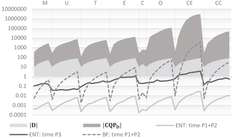
Figure 1: Results for systems in Tab. 2 (x-axis): # of leading diagnoses $|{\bf{D}}|$, associated size $|\mathbf{CQP}_{\bf{D}}|$ of CQP search space, and computation time (sec) required by phases P1+P2 and P3 for QSM ENT with threshold $t_{m}=0.01$ and brute force (BF) search (y-axis).

5 Conclusion

We present a search that addresses the optimal measurement (query) selection problem for sequential diagnosis and is applicable to any model-based diagnosis problem conforming to de Kleer and Williams (1987); Reiter (1987). In particular, we allow a query to be optimized along two dimensions, i.e. number of queries and cost per query. We show that the optimizations of these properties can be decoupled and considered in sequence. For a suitably restricted (still exponential) query search space (very close approximations of) global optima wrt. given query quality measures are found without any calls to an inference engine in negligible time for diagnosis problems of any size and complexity (given the precomputation of $\geq 2$ diagnoses is feasible). E.g. query search spaces of size up to $3$ million can be handled instantaneously ($<0.1$ sec). For the full search space, under reasonable assumptions, the globally optimal query wrt. a cost-preference measure can be found within 4 sec for up to $80$ leading diagnoses.

References

- Baader et al. [2003] F Baader, D Calvanese, D McGuinness, D Nardi, and P Patel-Schneider, (eds.). The Description Logic Handbook. Cambridge University Press, 2003.
- Brodie et al. [2003] M Brodie, I Rish, S Ma, and N Odintsova. Active probing strategies for problem diagnosis in distributed systems. In IJCAI, pp. 1337–1338, 2003.
- Bylander et al. [1991] T Bylander, D Allemang, M Tanner, and J Josephson. The computational complexity of abduction. Artif. Intell., 49:25–60, 1991.
- de Kleer and Raiman [1993] J de Kleer and O Raiman. How to diagnose well with very little information. In Working Notes of the 4th DX Workshop, pp. 160–165, 1993.
- de Kleer and Williams [1987] J de Kleer and B C Williams. Diagnosing multiple faults. Artif. Intell., 32:97–130, 1987.
- de Kleer and Williams [1989] J de Kleer and B C Williams. Diagnosis with behavioral modes. In IJCAI, pp. 1324–1330, 1989.
- de Kleer et al. [1992] J de Kleer, O Raiman, and M Shirley. One step lookahead is pretty good. In Readings in model-based diagnosis, pp. 138–142. Morgan Kaufmann, 1992.
- de Kleer [1991] J de Kleer. Focusing on probable diagnoses. In AAAI, pp. 842–848, 1991.
- Dressler and Struss [1996] O Dressler and P Struss. The consistency-based approach to automated diagnosis of devices. Principles of Knowl. Repr., pp. 269–314, 1996.
- Feldman et al. [2010] A Feldman, G M Provan, and A J C van Gemund. A model-based active testing approach to sequential diagnosis. JAIR, 39:301–334, 2010.
- Felfernig et al. [2004] A Felfernig, G Friedrich, D Jannach, and M Stumptner. Consistency-based diagnosis of configuration KBs. Artif. Intell., 152(2):213–234, 2004.
- Felfernig et al. [2009] A Felfernig, G Friedrich, K Isak, K Shchekotykhin, E Teppan, and D Jannach. Automated debugging of recommender user interface descriptions. Applied Intell., 31(1):1–14, 2009.
- Friedrich and Shchekotykhin [2005] G Friedrich and K Shchekotykhin. A General Diagnosis Method for Ontologies. In ISWC, pp. 232–246, 2005.
- Heckerman et al. [1995] D Heckerman, J S Breese, and K Rommelse. Decision-theoretic troubleshooting. Communications of the ACM, 38(3):49–57, 1995.
- Hyafil and Rivest [1976] L Hyafil and R L Rivest. Constructing optimal binary decision trees is NP-complete. Information processing letters, 5(1):15–17, 1976.
- Junker [2004] U Junker. QUICKXPLAIN: Preferred Explanations and Relaxations for Over-Constrained Problems. In AAAI, pp. 167–172, 2004.
- Kalyanpur et al. [2007] A Kalyanpur, B Parsia, M Horridge, and E Sirin. Finding all Justifications of OWL DL Entailments. In ISWC, pp. 267–280, 2007.
- Mateis et al. [2000] C Mateis, M Stumptner, D Wieland, and F Wotawa. Model-Based Debugging of Java Programs. In AADEBUG’00, 2000.
- Pattipati and Alexandridis [1990] K R Pattipati and M G Alexandridis. Application of heuristic search and information theory to sequential fault diagnosis. IEEE Trans. on Systems, Man, and Cybernetics, 20(4):872–887, 1990.
- Pencolé and Cordier [2005] Y Pencolé and M-O Cordier. A formal framework for the decentralised diagnosis of large scale discrete event systems and its application to telecommunication networks. Artif. Intell., 164(1):121–170, 2005.
- Pietersma et al. [2005] J Pietersma, A J C van Gemund, and A Bos. A model-based approach to sequential fault diagnosis. In IEEE Autotestcon, pp. 621–627. IEEE, 2005.
- Reiter [1987] R Reiter. A Theory of Diagnosis from First Principles. Artif. Intell., 32(1):57–95, 1987.
- Rodler et al. [2013] P Rodler, K Shchekotykhin, P Fleiss, and G Friedrich. RIO: Minimizing User Interaction in Ontology Debugging. In RR, pp. 153–167, 2013.
- Rodler [2015] Patrick Rodler. Interactive Debugging of Knowledge Bases. PhD thesis, Alpen-Adria Universität Klagenfurt, 2015. http://arxiv.org/pdf/1605.05950v1.pdf.
- Russell and Norvig [2010] S J Russell and P Norvig. Artif. Intell.: A Modern Approach. Pearson Education, 2010.
- Settles [2012] B Settles. Active Learning. Morgan and Claypool Publishers, 2012.
- Shakeri et al. [2000] M Shakeri, V Raghavan, K R Pattipati, and A Patterson-Hine. Sequential testing algorithms for multiple fault diagnosis. IEEE Trans. on Systems, Man, and Cybernetics, Part A, 30(1):1–14, 2000.
- Shchekotykhin et al. [2012] K Shchekotykhin, G Friedrich, P Fleiss, and P Rodler. Interactive Ontology Debugging: Two Query Strategies for Efficient Fault Localization. J. of Web Semantics, 12-13:88–103, 2012.
- Shchekotykhin et al. [2014] K Shchekotykhin, G Friedrich, P Rodler, and P Fleiss. Sequential diagnosis of high cardinality faults in knowledge-bases by direct diagnosis generation. In ECAI, pp. 813–818, 2014.
- Siddiqi and Huang [2011] S Siddiqi and J Huang. Sequential diagnosis by abstraction. JAIR, 41:329–365, 2011.
- Sirin et al. [2007] E Sirin, B Parsia, B Cuenca Grau, A Kalyanpur, and Y Katz. Pellet: A practical OWL-DL reasoner. J. of Web Semantics, 5(2):51–53, 2007.
- Stuckenschmidt [2008] H Stuckenschmidt. Debugging OWL Ontologies: Reality Check. In EON, pp. 1–12, 2008.
- Stumptner and Wotawa [1999] M Stumptner and F Wotawa. Debugging functional programs. In IJCAI, pp. 1074–1079, 1999.
- White et al. [2010] J White, D Benavides, D C Schmidt, P Trinidad, B Dougherty, and A R Cortés. Automated diagnosis of feature model configurations. J. Syst. Software, 83(7):1094–1107, 2010.
- Wotawa [2002] F Wotawa. On the relationship between model-based debugging and program slicing. Artif. Intell., 135(1-2):125–143, 2002.
- Zuzek et al. [2000] A Zuzek, A Biasizzo, and F Novak. Sequential diagnosis tool. MICPRO, 24(4):191–197, 2000.