Targeted Learning with Daily EHR Data

Abstract

Electronic health records (EHR) data provide a cost and time-effective opportunity to conduct cohort studies of the effects of multiple time-point interventions in the diverse patient population found in real-world clinical settings. Because the computational cost of analyzing EHR data at daily (or more granular) scale can be quite high, a pragmatic approach has been to partition the follow-up into coarser intervals of pre-specified length. Current guidelines suggest employing a ’small’ interval, but the feasibility and practical impact of this recommendation has not been evaluated and no formal methodology to inform this choice has been developed. We start filling these gaps by leveraging large-scale EHR data from a diabetes study to develop and illustrate a fast and scalable targeted learning approach that allows to follow the current recommendation and study its practical impact on inference. More specifically, we map daily EHR data into four analytic datasets using 90, 30, 15 and 5-day intervals. We apply a semi-parametric and doubly robust estimation approach, the longitudinal TMLE, to estimate the causal effects of four dynamic treatment rules with each dataset, and compare the resulting inferences. To overcome the computational challenges presented by the size of these data, we propose a novel TMLE implementation, the ’long-format TMLE’, and rely on the latest advances in scalable data-adaptive machine-learning software, xgboost and h2o, for estimation of the TMLE nuisance parameters.

keywords: Big data; Causal inference; Dynamic treatment regimes; EHR; Machine learning; Targeted minimum loss-based estimation.

1 Introduction

The availability of linked databases and compilations of electronic health records (EHR) has enabled the conduct of observational studies using large representative population cohorts. This data typically provides information on the nature of clinical visits (e.g, ambulatory, emergency department, email, telephone, acute inpatient hospital stay), medication dispensed, diagnoses, procedures, laboratory test results and any other information that is continuously generated from patients’ encounters with their healthcare providers. For instance, EHR-based cohort studies have been used to estimate the relative effectiveness of time-varying interventions in real-life clinical settings.

The advances in causal inference have provided a sound methodological basis for designing observational studies and assessing the validity of their findings. For example, the “new user design” [40] advocates for applying the same rigor and selection criteria used in RCT design to EHR-based observational studies [17, 19]. Moreover, advances in semi-parametric and empirical process theory have allowed for flexible data-adaptive estimation methods that can incorporate machine learning into analyses of comparative effectiveness. By lowering the risk of model misspecification, these data-adaptive approaches can further strengthen the validity of evidence based on observational studies. Finally, some of these semi-parametric approaches also allow drawing valid inference based on formal asymptotic results. For example, the recently proposed Targeted Minimum Loss-Based Estimation (TMLE) for longitudinal data [49, 35] – a doubly robust and locally-efficient substitution estimator.

While recent methodological advances have significantly improved the potential strength of evidence from observational studies, the practical tools for conducting such analyses have not kept up with the growing size of EHR data. In particular, implementation and application of machine learning to large scale EHR data has proved to be challenging [15, 27]. EHR data typically includes almost continuous event dates (e.g., data is updated daily), rather than the discrete event dates from interval assessments more common in epidemiologic cohort studies and many RCTs (e.g., data is updated every 3 months). To mitigate the high computing cost of analyzing EHR data at the daily (or more granular) scale, an analyst typically discretizes study follow-up by choosing a small number of cutoff time points. These cutoffs determine the duration of each follow-up time interval and the total number of analysis time points. The granular EHR data on each subject is then aggregated into interval-specific measurements for downstream analysis.

Current literature suggests choosing a small time interval [19] to define evenly spaced cutoff time points, however there are no clear guidelines for deciding on the optimal duration of this interval (referred to as the ’time unit’ from hereon). Moreover, in practice, the effect of selecting different time unit on causal inferences has not been previously examined within the same EHR cohort. Notably, the choice of a time unit is often driven by the computational complexity of the estimation procedure, as much as the subject-specific domain knowledge [27]. For example, in Neugebauer et al. [30] the authors applied longitudinal TMLE for estimating the comparative effectiveness of four dynamic treatment regimes by coarsening the daily EHR data into the 90-day time unit. However, such coarsening introduces measurement error, which can in turn lead to bias in the resulting effect estimates. For example, the treatment level assigned to a patient for one 90-day time-interval might misrepresent the actual treatment experienced. Intuitively, analyzing data as it is observed (using the original event dates) should improve causal inferences by avoiding the reliance on arbitrary coarsening algorithms.

In this paper, we propose a fast and scalable targeted learning implementation for estimating the effects of complex treatment regimes using EHR data coarsened with a time unit that can more closely (compared to current practice) approximate the original EHR event dates. We demonstrate the feasibility of the proposed approach and evaluate how the choice of progressively larger time units may effect inference by re-analyzing EHR data from a large diabetes comparative effectiveness study described in Neugebauer et al. [30]. We used the granular EHR data generated from the patient’s encounters with the healthcare system and discretized the patient-specific daily follow-up by mapping it into equally-sized time bins. In separate analyses, the time unit was varied from 90 days, down to 30, 15 and 5 days. These four time-units yielded four analytic datasets, each based on the same pool of subjects, but with a different level of follow-up coarsening as defined by selected time-unit. Notably, the 5-day time-unit produced a dataset that was nearly a replica of the original granular EHR dataset. We then applied an analogue of the double robust estimating equation method first proposed by Bang and Robins [1], similar to the TMLE described in van der Laan and Gruber [49], to each of these four datasets. We also compared our results to those obtained from the previous TMLE analysis based on 90-day time-unit in Neugebauer et al. [30].

The 90, 30, 15 and 5-day time-unit resulted in datasets with roughly 0.62, 1.81, 3.59 and 8.23 million person-time observations for the entire duration of the follow-up, respectively. The large number of person-time observations and the high computational complexity of our chosen estimation procedures required developing novel statistical software. We carried out our analysis by implementing a new R package, $\mathtt{stremr}$ [46], which streamlines the analysis of comparative effectiveness of static, dynamic and stochastic interventions in large-scale longitudinal data. As part of the $\mathtt{stremr}$ R package, we have implemented a computationally efficient version of the longitudinal TMLE, to which we refer as the long-format TMLE. Furthermore, for estimation of the nuisance parameters, we relied on the latest machine learning tools available in R language [38], such as the Extreme Gradient Boosting with $\mathtt{xgboost}$ [3] and fast and scalable machine learning with $\mathtt{h2o}$ [48]. Both of these packages implement a number of distributed and highly data-adaptive algorithms designed to work well in large data.

The contributions of this article can be summarized as follows. First, to the best of our knowledge, this is the first time the performance of longitudinal TMLE has been evaluated on the same EHR data under varying discretizations of the follow-up time. Furthermore, we present a novel and computationally efficient version of the longitudinal TMLE. We also present a possible application of the new $\mathtt{stremr}$ software which allowed us to analyze such large scale EHR data. Finally, we hope that our new software will help advance future reproducible research with EHR data and will contribute to research on time-unit selection and its effects on inference.

The remainder of this article is organized as follows. In Section 2, we describe our motivating research question. In Section 3 we formally describe the observed data, our statistical parameter and introduce a novel implementation of the longitudinal TMLE with data-adaptive estimation of its nuisance parameters. In Section 4, we describe our analyses, present the benchmarks for computing times with the $\mathtt{stremr}$ R package and present our analyses results. Finally, we conclude with a discussion in Section 5. Additional materials and results are provided in our Web Supplement.

2 Motivating study: comparative effectiveness of dynamic regimes in diabetes care

The diabetes study and context that motivated this work was previously described in Neugebauer et al. [30]. Briefly, it has long been hypothesized that aggressive glycemic control is an effective strategy to reduce the occurrence of common and devastating microvascular and macrovascular complications of type 2 diabetes (T2DM). A major goal of clinical care of T2DM is minimization of such complications through a variety of pharmacological treatments and interventions to achieve recommended levels of glucose control. The progressive nature of T2DM results in frequent revisiting of treatment decisions for many patients as glycemic control deteriorates. Widely accepted stepwise guidelines start treatment with metformin, then add a secretagogue if control is not reached or deteriorates. Insulin or (less frequently) a third oral agent is the next step. Thus, it is common for T2DM patients to be on multiple glucose-lowering medications.

Current recommendations specify target hemoglobin A1c of $<7\%$ for most patients [26, 44]. However, evidence supporting the effectiveness of a blanket recommendation is inconsistent across several outcomes [39, 9, 14, 20], especially when intensive anti-diabetic therapy is required. The effects of intensive treatment remain uncertain, and the optimal target levels of A1c for balancing benefits and risks of therapy are not clearly defined. Furthermore, no additional major trials addressing these questions are underway.

For these reasons, using the electronic health records (EHR) from patients of seven sites of the HMO Research Network [57], a large retrospective cohort study of adults with T2DM was conducted to evaluate the impact of various glucose-lowering strategies on several clinical outcomes. More specifically, the original analyses were based on TMLE and Inverse Probability Weighting estimation approaches using EHR data coarsened with the 90-day time unit to contrast cumulative risks under the following four treatment intensification (TI) strategies denoted by $d_{\theta}$: ’patient initiates TI at the first time her A1c level reaches or drifts above $\theta$% and patient remains on the intensified therapy thereafter’ with $\theta=$7, 7.5, 8, or 8.5. Here, we report on secondary analyses to evaluate the impact of the same glucose-lowering strategies on the development or progression of albuminuria, a microvascular complication in T2DM using a novel TMLE implementation and smaller time units.

3 Data and Modeling Approaches

Below, we first describe the structure of the analytic dataset that results from coarsening EHR data based on a particular choice of time unit.

3.1 Data structure and causal parameter

The observed data on each patient in the cohort consist of measurements on exposure, outcome, and confounding variables updated at regular time intervals between study entry and until each patient’s end of follow-up. The time (expressed in units of 90, 30, 15 or 5 days) when the patient’s follow-up ends is denoted by $\tilde{T}$ and is defined as the earliest of the time to failure, i.e., albuminuria development or progression, denoted by $T$ or the time to a right-censoring event denoted by $C$. The following three types of right-censoring events experienced by patients in the study were distinguished: the end of follow-up by administrative end of study, disenrollment from the health plan and death. For patients with normoalbuminuria at study entry, i.e., microalbumin-to-creatinine ratio (ACR) $<$30, we defined failure as an ACR measurement indicating either microalbuminuria (ACR 30 to 300) or macroalbuminuria (ACR$>$300). For patients with microalbuminuria at study entry, we defined failure as an ACR measurement indicating macroalbuminuria. Addition inclusion and exclusion criteria described in Neugebauer et al. [30] yielded the final sample size $n=51,179$.

At each time point $t=0,\ldots,\tilde{T}$, the patient’s exposure to an intensified diabetes treatment is represented by the binary variable $A^{T}(t)$, and the indicator of the patient’s right-censored status at time $t$ is denoted by $A^{C}(t)$. The combination $A(t)=(A^{T}(t),A^{C}(t))$ is referred to as the action at time $t$. At each time point $t=0,\ldots,\tilde{T}$, covariates, such as A1c measurements (others are listed in Table I of Neugebauer et al. [32]), are denoted by the multi-dimensional variable $L(t)$ and defined from EHR measurements that occur before the action at time $t$, $A(t)$, or are otherwise assumed not to be affected by the actions at time $t$ or thereafter, ($A(t),A(t+1),\ldots$). In addition, data collected at each time $t$ includes an outcome process denoted by $Y(t)$ - an indicator of failure prior to or at $t$, formally defined as $Y(t)=I(T\leq t)$. By definition, the outcome is thus missing at $t=\tilde{T}$ if the person was right-censored at $t$.

To simplify notation, we use over-bars to denote covariate and exposure histories, e.g., a patient’s exposure history through time $t$ is denoted by $\bar{A}(t)=(A(0),\ldots,A(t))$. We assume the analytic dataset is composed of $n$ independent and identically distributed (iid) realizations $(O_{i}:i=1,\ldots,n)$ of the following random variable $O=(\bar{L}(\tilde{T}),\bar{A}(\tilde{T}),\bar{Y}(\tilde{T}-1),(1-A^{C}(\tilde{T}))Y(\tilde{T}))\sim P$. We also assume that each $O_{i}$ is drawn from distribution $P$ belonging to some model $\mathcal{M}$. By convention, we extend the observed data structure using first $Y_{i}(\tilde{T}_{i})=0$ if $A_{i}^{C}(\tilde{T}_{i})=1$ and then $O_{i}(t)=O_{i}(\tilde{T}_{i})$ for $t>\tilde{T}_{i}$. Note that these added degenerate random variables will not be used in the practical implementation of our estimation procedure, yet they will allow us to simplify the presentation in the following section. In particular, this convention implies that whenever $Y(\tilde{T}_{i})=1$, the outcomes $Y_{i}(t)$ are deterministically set to $1$ for all $t>\tilde{T}_{i}$.

One common way to store $(O_{1},\ldots,O_{n})$ in a computer is with the so-called “long-format” dataset, where each row contains a record of a single person-time observation $O_{i}(t)=(L_{i}(t),A_{i}(t),Y_{i}(t))$, for some $i\in\{1,\ldots,n\}$ and $t\in\{0,\ldots,\tilde{T}_{i}\}$. For time-to-event data, the long-format can be especially convenient, since only the relevant (non-degenerate) information is kept, while all degenerate observation-rows such that $t>\tilde{T}_{i}$ are typically discarded. An alternative way to store the same analytic dataset is by using the so-called “wide-format”, which includes values for the degenerate part of the observed data structure $O_{i}(t)$ for $\tilde{T}_{i}<t\leq K$, where $K=\max(\tilde{T}_{i}:i=1,...,n)$. For the remainder of this paper we assume that data are stored in long-format.

In this study, we aim to evaluate the effect of dynamic treatment interventions on the cumulative risk of failure at a pre-specified time point $t_{0}$. The dynamic treatment interventions of interest correspond to treatment decisions made according to given clinical policies for initiation of an intensified therapy based on the patient’s evolving A1c level. These policies denoted by $d_{\theta}$ were described above. Formally, these policies are individualized action rules [53] defined as a vector function $\bar{d}_{\theta}=(d_{\theta,0},\ldots,d_{\theta,t_{0}})$ where each function, $d_{\theta,t}$ for $t=0,\ldots,t_{0}$, is a decision rule for determining the action regimen (i.e., a treatment and right-censoring intervention) to be experienced by a patient at time $t$, given the action and covariate history measured up to a given time $t$. More specifically here, we consider the action rule $(L(t),A(t-1))\mapsto d_{\theta,t}(L(t),A(t-1))\in\{0,1\}\times\{0\}$ as a function for assigning the treatment action $A(t)$. Note that these rules are restricted to set the censoring indicators $A^{C}(t)=0$. Furthermore, at each time $t$, we define the dynamic rule $d_{\theta,t}$ by setting $A^{T}(t)=0$ if and only if the patient was not previously treated with an intensified therapy (i.e., $A(t-1)=0$) and the A1c level at time $t$ (an element of $L(t)$) was lower than or equal to $\theta$, and, otherwise, setting $A^{T}(t)=1$. Finally, for each observation $O_{i}$, we define the treatment process $\bar{A}_{i}^{\theta}(t)=(A_{i}^{\theta}(0),\ldots,A_{i}^{\theta}(t))$ as the treatment sequence that would result from sequentially applying the previous action rules, i.e., $(d_{\theta,0}(L_{i}(0)),\ldots,d_{\theta,t}(L_{i}(t),A_{i}^{\theta}(t-1)))$, starting at time $0$ through $t$. Note that the rules defined by $\bar{d}_{\theta}$ are deterministic for a given $O_{i}$ and thus $\bar{A}_{i}^{\theta}$ is fixed conditional on the event $(O_{i}=o_{i})$. For notation convenience, we also set $\bar{A}_{i}^{\theta}(t)=\bar{A}_{i}^{\theta}(\tilde{T}_{i})$, for $t>\tilde{T}_{i}$, noting that, in practice, $\bar{A}_{i}^{\theta}(t)$ will be evaluated only when $t\leq\tilde{T}_{i}$ and can be set as arbitrary for all other $t$.

Suppose $Y_{\bar{d}_{\theta}}(t_{0})$ for $\theta=\theta_{1},\theta_{2}$ denotes a patient’s potential outcome at time $t_{0}$ had she been treated between study entry and time $t_{0}$ according to the decision rule $\bar{d}_{\theta}$. Note that the corresponding sequence of treatment interventions is not necessarily equal to $\bar{A}_{i}^{\theta}(t_{0})$. The parameter of interest denoted by $\psi^{\theta_{1},\theta_{2}}(t_{0})$ is then defined as the causal risk difference between the cumulative risks of two distinct dynamic treatment strategies $\bar{d}_{\theta_{1}}$ and $\bar{d}_{\theta_{2}}$ at $t_{0}$: $\psi^{\theta_{1},\theta_{2}}(t_{0})=\psi^{\theta_{1}}(t_{0})-\psi^{\theta_{2}}(t_{0}),$ where $\psi^{\theta}(t_{0})=P(Y_{\bar{d}_{\theta}}(t_{0})=1)$, i.e., the cumulative risk associated with rule $\bar{d}_{\theta}$ at $t_{0}$. The above definition of the causal parameter of interest relies on the counterfactual statistical framework, which is omitted here for brevity. We refer the reader to earlier work in Neugebauer et al. [28, Appendices B and D] and van der Laan and Petersen [53] for a detailed description of the relevant concepts.

3.2 Identifiability and the statistical parameter of interest

As discussed in the next paragraph, identifiability of the causal parameter with the observational data relies on at least two assumptions: no unmeasured confounding and positivity [28, Appendix C]. If the counterfactual outcomes are not explicitly defined based on the more general structural framework through additional explicit assumptions encoded by a causal diagram [34], then an additional consistency assumption is made [56].

Without loss of generality, suppose that we are interested in estimating the cumulative risk $\psi^{\theta}(t_{0})$ at $t_{0}=1$ under fixed dynamic regimen $\bar{d}_{\theta}=(d_{\theta,0},d_{\theta,1})$. Define $L^{\prime}(k)=(L(k),\bar{O}(k-1))$, for $k=0,\ldots,t_{0}$, where by convention $(A(-1),L(-1))$ is an empty set and $Y(-1)=0$. Let $o=(\bar{l}(\tilde{t}),\bar{a}(\tilde{t}),\bar{y}(\tilde{t}))$ denote a particular fixed realization of $O$. We can now define the following recursive sequence of expectations:

$$Q_{1}(a,l)=E_{P}(Y(1)|A(1)=a,L^{\prime}(1)=l),$$

$$Q_{0}(a,l) = E_{P}(Q_{1}(A^{\theta}(1),L^{\prime}(1))|A(0)=a,L^{\prime}(0)=l)$$

$$Q_{-1}=E_{P}(Q_{0}(A^{\theta}(0),L^{\prime}(0)),$$

where we remind that $(A^{\theta}(0),A^{\theta}(1))$ was previously defined as the sequence of treatments $A^{\theta}(0)=d_{\theta,0}(L(0))$ and $A^{\theta}(1)=d_{\theta,1}(\bar{L}(1),A^{\theta}(0))$. Note that, by definition $Q_{1}$ is 1 whenever $Y(0)=1$, since in this case $Y(1)$ is degenerate.

Remark 1.

Each $Q_{k}$, for $k=-1,0$, is defined by taking the previous conditional expectation, $Q_{k+1}$, evaluating it at $A^{\theta}(k+1)$ and $L^{{}^{\prime}}(k+1)$ and then marginalizing over the intermediate covariates $L^{{}^{\prime}}(k+1)$.

Under the identifiability assumptions mentioned above, we show in Web Supplement A that the statistical parameter $\Psi^{\theta}(t_{0})(P)=Q_{-1}$ is equal to the causal cumulative risk $\psi^{\theta}(t_{0})$ for dynamic rule $\bar{d}_{\theta}$. We note that the above representation of $Q_{-1}$ is analogous to the iterative conditional expectation representation used in van der Laan and Gruber [49], with one notable difference: our parameter evaluates $Q_{1}$ and $Q_{0}$ with respect to the latest values of the counterfactual treatment, $A^{\theta}(1)$ and $A^{\theta}(0)$, respectively. This is in contrast to the iterative conditional expectations in van der Laan and Gruber [49], where conditioning in $Q_{1}$ would be evaluated with respect to the entire counterfactual history of exposures $\bar{A}^{\theta}(1)$. As we show in Web Supplement A, these two parameter representations happen to be equivalent. However, our particular target parameter representation above will allow us to develop a TMLE that is computationally faster and more scalable to a much larger number of time-points.

We introduce the following notation, which will be useful for the description of the TMLE in next section: let $Q=(Q_{1},Q_{0})$ and, for $k=0,1$, define the treatment mechanism $g_{A(k)}(a(k)|l^{\prime}(k))=P(A(k)=a(k)|L^{{}^{\prime}}(k)=l^{\prime}(k))$, i.e., the conditional probability that $A(k)$ is equal to $a(k)$, conditional on events $L^{\prime}(k)$ being set to some fixed history $l^{\prime}(k)$. Finally, let $g=(g_{A(0)},g_{A(1)})$.

3.3 Long-format TMLE for time-to-event outcomes

Doubly robust approaches allow for consistent estimation of $\Psi^{\theta}(t_{0})(P)$ even when either the outcome model for $Q$ or the exposure model for $g$ is misspecified. Among the class of doubly robust estimators, those that are based on the substitution principle, such as the longitudinal TMLE in van der Laan and Gruber [49], might be preferable, since the substitution principle may offer improvements in finite sample behavior of an estimator. The TMLE described in van der Laan and Gruber [49] is an analogue of the double robust estimating equation method presented in Bang and Robins [1]. While there are several possible ways to implement the longitudinal TMLE procedure (e.g., Stitelman et al. [47], van der Laan and Gruber [49], Schwab et al. [43]), our implemented version, referred to as “long-format TMLE”, has been adapted to work efficiently with large scale time-to-event EHR datasets.

As a reminder, for each subject $i$, we defined $L^{\prime}_{i}(k)$ to include $i$’s entire covariate history up to time-point $k$, in addition to $L_{i}(k)$ itself. However, due to the curse of dimensionality, estimating $Q_{k}$ based on all $L^{\prime}(k)$, when $k$ is sufficiently large and $L(k)$ is high-dimensional, will generally result in a poor finite-sample performance. Thus, to control the dimensionality , we replace $L^{\prime}(k)$ with a user-defined summary $f_{k}(L^{\prime}(k))$, where $f_{k}(\cdot)$ is an arbitrary mapping $(\bar{L}(k),\bar{A}(k-1))\mapsto R^{d}$ such that $d$ is fixed for all $k=0,\ldots,\max(\tilde{T})$. For example, in our data analyses presented in the following sections we defined the mapping $f_{k}(L^{\prime}(k))$ as $(L(0),L(k),A(k-1))$. This approach allows the practitioner to control the dimensionality of the regression problem when fitting each $Q_{k}$ model. Furthermore, by forcing all relevant confounders for time-point $k$ to be defined in a single person-time row via the mapping $f_{k}(\cdot)$ (i.e., $(f_{k}(\cdot),A_{i}(k),Y_{i}(k))$), we can also simplify the implementation of the iterative part of TMLE algorithm that fits the initial model for $Q_{k}$, as we describe next.

Applying the mappings $f_{k}(\cdot)$ to our observed data on $n$ subjects, $(O_{1},\ldots,O_{n})$, results in a new, reduced, long-format representation of the data, where each row of the reduced dataset is defined by the following person-time observation $(f_{k}(L^{\prime}_{i}(k)),A_{i}(k),Y_{i}(k))$, for some $i\in\{1,\ldots,n\}$ and $k\in\{0,\ldots,\tilde{T}_{i}\}$. For example, for subject $i$ with $\tilde{T}_{i}=0$, the entire reduced representation of $O_{i}$ consists of just a single person-time row $(f_{0}(L_{i}(0)),A_{i}(0),Y_{i}(0))$. Our proposed TMLE algorithm, outlined below, will work directly with this reduced long-format representation of $(O_{1},...,O_{n})$. The algorithm relies on the representation of $\Psi^{\theta}(t_{0})(P)$ from the previous section, where one makes predictions based on only the last treatment value for each time-point. This in turn allows us to keep the input data in the reduced long-format at all times, substantially lowering the memory footprint of the procedure.

We now describe the long-format TMLE algorithm for estimating parameter $\Psi^{\theta}(t_{0})(P)$ indexed by the fixed dynamic regimen $\bar{d}_{\theta}=(d_{\theta,0},...,d_{\theta,t_{0}})$, where for simplicity, we let $t_{0}=1$. A more detailed description of this TMLE is also provided in the Web Supplement B. Briefly, the algorithm proceeds recursively by estimating each $Q_{k}$ in $Q$, for $k=1,0$. Prior to that, we instantiate a new variable $\tilde{Q}_{(k+1)}=Y(k)$, for $k=0,\ldots,\tilde{T}$ and we make one final modification to our reduced long-format dataset by adding a new column of subject-specific cumulative weight estimates, defined for each row $k$ as $\hat{wt}(k)=\prod_{j=0}^{k}\frac{I(\bar{A}(j)=\bar{A}^{\theta}(j))}{\hat{g}_{A(j)}(O)}$, where $k=0,\ldots,\tilde{T}$ and $\hat{g}_{A(j)}$ is the estimator of $g_{A(j)}$ at $j$. For iteration $k=1$, one starts by obtaining an initial estimate $\hat{Q}_{k}$ of $Q_{k}$ by regressing $\tilde{Q}_{(k+1)}$ against $(A(k),f_{k}(L^{\prime}(k)))$ based on some parametric (e.g., logistic) model, for all subjects such that $\tilde{T}\geq k$ and $A^{C}(k)=0$ (i.e., this fit is performed among subjects who were at risk for the event at time $k$). Alternatively, the regression fit can be obtained by using a subset of subjects such that $A(k)=A^{\theta}(k)$ or based on a data-adaptive estimation procedure as discussed later. Next, one estimates the intercept $\varepsilon^{k}$ with an intercept-only logistic regression for the outcome $\tilde{Q}_{(k+1)}$ using the offset $\mbox{logit}\hat{Q}_{k}(A^{\theta}(k),f_{k}(L^{\prime}(k)))$, and the weights $\hat{wt}(k)$, where $\mbox{logit}(x)=\log\left(\frac{x}{1-x}\right)$. The last regression defines the TMLE update $\hat{Q}_{k}^{*}$ of $\hat{Q}_{k}$ as $\mbox{expit}\left(\mbox{logit}\hat{Q}_{k}(a^{\theta}(k),f_{k}(l^{\prime}(k)))+\hat{\varepsilon}^{k}\right)$, for any realization $(a^{\theta}(k),l^{\prime}(k))$ and $\mbox{expit}(x)=\frac{1}{1+e^{-x}}$. Finally, if $k>0$, for all subjects such that $\tilde{T}\geq k$, we compute the TMLE update, defined as $\hat{Q}_{k}^{*}(A^{\theta}(k),f_{k}(L^{\prime}(k)))$, and use this update to over-write the previously defined instance of $\tilde{Q}_{k}$. Note that $\tilde{Q}_{k}$ remains set to $Y(k-1)$ for all subjects with $\tilde{T}<k$. The illustration of this over-writing scheme for $\tilde{Q}_{k}$ is also presented in Figure 3.1 for iteration $k=1$, using a toy example for three hypothetical subjects. The same procedure is now repeated for iteration $k=0$, using the outcome $\tilde{Q}_{(k+1)}$, resulting in TMLE update $\hat{Q}_{k}^{*}$, for all subjects $i=1,\ldots,n$. Finally, the TMLE of $\Psi^{\theta}(t_{0})(P)=Q^{-1}$ is defined as $\hat{\Psi}^{\theta}(t_{0})=\frac{1}{n}\sum_{i=1}^{n}\hat{Q}_{0}^{*}(A_{i}^{\theta}(0),f_{0}(L^{\prime}_{i}(0)))$. TMLE estimate of the causal RD $\psi^{\theta_{1},\theta_{2}}(t_{0})$ can be now evaluated as $\hat{\Psi}^{\theta_{1}}(t_{0})(P)-\hat{\Psi}^{\theta_{2}}(t_{0})(P)$, where the above described procedure is carried out separately to estimate $\Psi^{\theta_{1}}(t_{0})(P)$ and $\Psi^{\theta_{2}}(t_{0})(P)$, for rules $\bar{d}_{\theta_{1}}$ and $\bar{d}_{\theta_{2}}$, respectively.

Note that in above description, each initial estimate $\hat{Q}_{k}$ can be obtained by either stratifying the subjects based on $A(k)=A^{\theta}(k)$ (referred to as “stratified TMLE”) or by pooling the estimation among all subjects at risk of event at time $k$ (referred to as “pooled TMLE”). Furthermore, in our data analyses described in Section 4, we use the stratified TMLE procedure. Finally, the inference can be obtained using the approach described in our Web Supplement C, based on the asymptotic results from prior papers.

1) Input data with initialized $\tilde{Q}_{(t+1)}$ values:

$i$	$t$	$\tilde{T}$	$f_{t}(L^{\prime}(t))$	$A^{C}(t)$	$Y(t)$	$\tilde{Q}_{(t+1)}$	$\hat{Q}_{t}^{*}$
$1$	$0$	$0$	.	0	$1$	$1$	NA
$2$	$0$	$1$	.	0	$0$	$0$	NA
$2$	$1$	$1$	.	0	$1$	$1$	NA
3	0	1	.	0	0	0	NA
3	1	1	.	1	NA	NA	NA

2) TMLE updates $\hat{Q}_{k}^{*}$ of $Q_{k}$ evaluated at iteration $k=1$:

$i$	$t$	$\tilde{T}$	$f_{t}(L^{\prime}(t))$	$A^{C}(t)$	$Y(t)$	$\tilde{Q}_{(t+1)}$	$\hat{Q}_{t}^{*}$
$1$	$0$	$0$	.	0	$1$	$1$	NA
$2$	$0$	$1$	.	0	$0$	$0$	NA
$2$	$1$	$1$	.	0	$1$	$1$	$\hat{Q}_{1,i}^{*}$
3	0	1	.	0	0	0	NA
3	1	1	.	1	NA	NA	$\hat{Q}_{1,i}^{*}$

3) Updated $\tilde{Q}_{(t+1)}$ values at the end of iteration $k=1$:

$i$	$t$	$\tilde{T}$	$f_{t}(L^{\prime}(t))$	$A^{C}(t)$	$Y(t)$	$\tilde{Q}_{(t+1)}$	$\hat{Q}_{t}^{*}$
$1$	$0$	$0$	.	0	$1$	$1$	NA
$2$	$0$	$1$	.	0	$0$	$\hat{Q}_{1,i}^{*}$	NA
$2$	$1$	$1$	.	0	$1$	$1$	$\hat{Q}_{1,i}^{*}$
3	0	1	.	0	0	$\hat{Q}_{1,i}^{*}$	NA
3	1	1	.	1	NA	NA	$\hat{Q}_{1,i}^{*}$

Figure 3.1: Illustration of the long-format TMLE updating step for the outcome $\tilde{Q}_{(t+1)}$ at iteration $k=1$ for three subjects $i=1,2,3$. Note that the TMLE update $\hat{Q}_{1,i}^{*}=\hat{Q}_{1}^{*}(A_{i}^{\theta}(1),f_{1}(L_{i}^{\prime}(1)))$ is also defined for the censored subject $i=3$ at $k=1$.

3.4 Data-adaptive estimation via cross-validation

The double-robustness property of the TMLE means that its consistency hinges on the crucial assumption that at least one of the two nuisance parameters ($g$, $Q$) is estimated consistently. Current guidelines suggest that the nuisance parameters, such as propensity scores, should be estimated in a flexible and data-adaptive manner [19, 31, 15]. However, traditionally in observational studies, these nuisance parameters have been estimated based on logistic regressions, with main terms and interaction terms often chosen based on the input from subject matter experts [42, 28, 2, 6, 18]. In contrast, a data-adaptive estimation procedure provides an opportunity to learn complex patterns in the data which could have been overlooked when relying on a single parametric model.

For instance, improved finite-sample performance from data-adaptive estimation of the nuisance parameters has been previously noted with Inverse Probability Weighting (IPW) estimation, a propensity score-based alternative to TMLE [31]. It has been suggested that problems with parametric modeling approaches can arise even in studies with no violation of the positivity assumption. For example, the predicted propensity scores from the misspecified logistic models might be close to 0 or 1, resulting in unwarranted extreme weights which could be avoided with data-adaptive estimation. Similarly, these extreme weights may also lead to finite-sample instability for doubly-robust estimation approaches, such as the long-format TMLE. These considerations provide further motivation for the use of the data-adaptive estimation procedures.

Many machine learning (ML) algorithms have been developed and applied for data-adaptive estimation of nuisance parameters in causal inference problems [25, 22, 58]. However, the choice of a single ML algorithm over others is unlikely to be based on real subject-matter knowledge, since: “in practice it is generally impossible to know a priori which [ML procedure] will perform best for a given prediction problem and data set” van der Laan et al. [54]. To hedge against erroneous inference due to arbitrary selection of a single algorithm, an ensemble learning approach known as discrete Super Learning (dSL) [54, 37] can be utilized. This approach selects the optimal ML procedure among a library of candidate estimators. The optimal estimator is selected by minimizing the estimated expectation of a user-specified loss function (e.g., the negative log-likelihood loss) [21]. Cross-validation is used to assess an expected loss associated with each candidate estimator, which protects against overfitting and ensures that the final selected estimator (called the ’discrete super learner’) performs asymptotically as well (in terms of the expected loss) as any of the candidate estimators considered [10]. Because of the general asymptotic and finite-sample formal dSL results, in this work we favor the approach of super learning over other existing ensemble learning approaches.

Prior applications of super learning in R [36] have noted the high computational cost of aggressive super learning, especially for large datasets (e.g., dSL library contains a large number of computationally costly ML algorithms) [15, 27]. Because of these limitations, which are also compounded by the choice of a smaller time unit in our study, we implemented a new version of the discrete super learner, the $\mathtt{gridisl}$ R package [45]. This R package is utilized for estimation of the TMLE nuisance parameters by the R package $\mathtt{stremr}$. Below, we describe how $\mathtt{gridisl}$ builds on the latest advances in scalable machine learning software, $\mathtt{xgboost}$ [3] and $\mathtt{h2o}$ [48], which makes it feasible to conduct more aggressive super learning in EHR-based cohort studies with small time units.

In our implementation of the discrete super learner, we focus on the negative log-likelihood loss function. The candidate machine learning algorithms that can be included in our ensembles are distributed high-performance $\mathtt{xgboost}$ and $\mathtt{h2o}$ implementations of the following algorithms: random forests (RFs), gradient boosting machines (GBMs) [12, 3, 4], logistic regression (GLM), regularized logistic regression, such as, LASSO, ridge and elastic net [59, 11]. GBM is an automated and data-adaptive algorithm that can be used with large number of covariates to fit a flexible non-parametric model. For overview of GBMs we refer to Hastie et al. [16]. The advantage of procedures like classification trees and GBM is that they allow us to search through a large space of model parameters, accounting for the effects of many covariates and their interactions, thereby reducing bias in the resulting estimator regardless of the distribution of the data that defined the true values of the nuisance parameters. The large number of possible tuning parameters available for the estimation procedures in our ensemble required conducting a grid search over the space of such parameters. We note that $\mathtt{gridisl}$ leverages the internal cross-validation implemented in $\mathtt{h2o}$ and $\mathtt{xgboost}$ R packages for additional computational efficiency.

4 Analysis

time-unit (day)	$n$ for $\hat{g}$	GLM $\hat{g}$	dSL $\hat{g}$	GLM $\hat{Q}^{*}$	dSL $\hat{Q}^{*}$
90	0.6M	0.05	4.95	0.06	0.81
30	1.8M	0.10	14.69	0.17	2.38
15	3.6M	0.17	28.03	0.34	4.67
5	8.2M	0.41	13.43	1.11	13.94

Table 1: Benchmarks for $\mathtt{stremr}$ with compute time for $\hat{g}$ and TMLE $\hat{Q}^{*}$ reported separately for parametric approach with logistic main-term models (GLM $\hat{g}$ and GLM $\hat{Q}^{*}$) and data-adaptive approach with discrete super learning (dSL $\hat{g}$ and dSL $\hat{Q}$). The running times are displayed in hours.

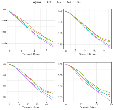
Figure 4.1: TMLE survival estimates for data-adaptive modeling approach for $Q$ and $g$, contrasting four dynamic interventions $(d_{7.0},d_{7.5},d_{8.0},d_{8.5})$ for 90 day (top-left panel), 30 day (top-right panel), 15 day (bottom-left panel) and 5 day (bottom-right panel) time-unit over two years of follow-up.

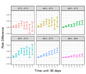
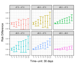
Figure 4.2: TMLE estimates of cumulative RDs with point-wise 95% CIs, contrasting four dynamic interventions $(d_{7.0},d_{7.5},d_{8.0},d_{8.5})$ for 90 day (left panel) and 30 day (right panel) time-unit over two years of follow-up.

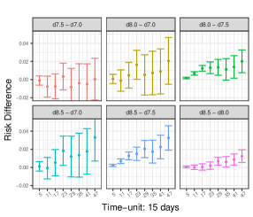
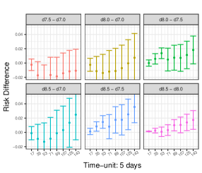
Figure 4.3: TMLE estimates of cumulative RDs with point-wise 95% CIs, contrasting four dynamic interventions $(d_{7.0},d_{7.5},d_{8.0},d_{8.5})$ for 15 day (left panel) and 5 day (right panel) time-unit over two years of follow-up.

In this section, we demonstrate a possible application of our proposed targeted learning software. We show that the $\mathtt{stremr}$ and $\mathtt{gridisl}$ R packages provide fast and scalable software for the analyses of high-dimensional longitudinal data. We estimate the effects of four dynamic treatment regimes on a time-to-event outcome using EHR data from the diabetes cohort study described in Sections 2 and 3.1. These analyses are based on large EHR cohort study, using four progressively smaller time units (i.e., four nested discretizations of the same follow-up data). For instance, the choice of the smaller time unit might more closely approximate the original EHR daily event dates, as it is the case in our application. We also evaluate the practical impact of these four progressively smaller time units on inferences. Finally, we compare the long-format TMLE results to those obtained from IPW estimator. All results are also compared to prior published findings from alternate IPW and TMLE analyses.

The choice of time-unit of 90, 30, 15, and 5 days results in four analytic datasets, each constructed by applying the SAS macro $\mathtt{\%\_MSMstructure}$ [23] to coarsen the original EHR data. The maximum follow-up in each dataset is subsequently truncated to the first two years, i.e., 8 quarters, 24 months, 48 15-day intervals, and 144 5-day intervals, respectively. For each analytic dataset, we evaluate the counterfactual cumulative risks at $t_{0}$ associated with four treatment intensification strategies, with $t_{0}$ fixed to $8$ distinct time points. That is, for the 90-day (resp. 30-day) analytic dataset, $\Psi^{\theta}(t_{0})(P)$ is estimated for $t_{0}=0,1,\ldots,7$ (resp. $t_{0}=2,5,\ldots,23$) and $\theta=7,7.5,8,8.5$. Similarly, for the 15-day (resp. 5-day) analytic dataset, $\Psi^{\theta}(t_{0})(P)$ is estimated for $t_{0}=5,10,\ldots,47$ (resp. $t_{0}=17,35,\ldots..,143)$ and $\theta=7,7.5,8,8.5$.

With each of the four analytic datasets and for each of the 32 target cumulative risks, we evaluate the following two estimators: the stratified long-format TMLE (Section 3.3) and a bounded IPW estimator (based on a saturated MSM for counterfactual hazards [31]). The TMLE and IPW estimators are implemented based on unstabilized and stabilized IP weights truncated at 200 and 40, respectively [5]. Each of the two estimators above uses two alternative strategies for nuisance parameter estimation: a-priori specified logistic regression models (parametric approach) and discrete super learning with 10-fold cross-validation (data-adaptive approach).

4.1 Nuisance parameter estimation approaches

For the parametric approach, the estimators of each $Q_{k}$ and $g_{A(k)}$, for $k=0,\ldots,t_{0}$, are based on separate logistic regression models that include main terms for all baseline covariates $L(0)$, the exposures $(A(k),A(k-1))$ and the most recent measurement of time-varying covariates $L(k)$, i.e., the reduced dataset is defined with $f_{k}(L^{\prime}(k))=(L(0),L(k),A(k-1))$. This covariate selection approach results in approximately 150 predictors for each regression model for $Q_{k}$ and $g_{A(k)}$, at each time point $k$. In addition, estimation of $g$ relies on fitting separate logistic models for treatment initiation and continuation. Furthermore, logistic models for two types of right-censoring events (health plan disenrollment and death) are fit separately, while it is assumed that right-censoring due to end of the study is completely at random (i.e., we use an intercept-only logistic regression). Each of the logistic models for estimating $g$ are fit by pooling data over all time-points $k=0,\ldots t_{0}$. Furthermore, the same sets of predictors that are used for estimation of $Q_{k}$ are also included in estimation of $g$, in addition to a main term for the value of time $k$. Finally, for $30$, $15$ and $5$ day time units, these logistic models also include the indicators that the follow-up time $k$ belongs to a particular two-month interval.

Remark 2.

The $\mathtt{\%\_MSMstructure}$ SAS macro [23] implements automatic imputation of the missing covariates and creates indicators of imputed values. The indicators of imputation are also included in each $L(k)$. The documentation for the SAS macro provides a detailed description of the implemented schemes for imputation.

For the data-adaptive estimation approach, each of the above-described logistic model-based estimators is replaced with a distinct discrete super learner. Each discrete super learner uses the same set of predictors that are included in the corresponding model from the parametric approach. The replication R code for the specification of each dSL is available from the following github repository: www.github.com/osofr/stremr.paper. In short, for estimation of each component of $g$, for 90, 30 and 15 day time-unit, the dSL uses the following ensemble of 89 distributed (i.e., parallelized) estimators that are each indexed by a particular tuning parameter choice: Random Forests (RFs) with $\mathtt{h2o}$ (8); Gradient Boosting Machines (GBMs) with $\mathtt{h2o}$ (1); GBMs with $\mathtt{xgboost}$ (18); Generalized Linear Models (GLMs) with $\mathtt{h2o}$ (2); and regularized GLMs with $\mathtt{h2o}$ (60). For 5 day time-unit, the dSL for each component of $g$ uses the following smaller ensemble of 20 estimators: RFs with $\mathtt{h2o}$ (1); GBMs with $\mathtt{h2o}$ (1); GBMs with $\mathtt{xgboost}$ (1); GLMs with $\mathtt{h2o}$ (2); and regularized GLMs with $\mathtt{h2o}$ (15). An abbreviated discussion of some of the tuning parameters that index the ML algorithms considered is provided in Remark 4. To obtain discrete super learning estimates for each component of $Q=(Q_{k}:k=0,\ldots,t_{0})$, we rely solely on the candidate estimators available in the $\mathtt{xgboost}$ R package because of computational constraints. Specifically, the dSL ensemble for each $Q_{k}$, for all four analytic datasets, is restricted to the following 8 estimators: GBMs with $\mathtt{xgboost}$ (3); GLMs with $\mathtt{xgboost}$ (1); and regularized GLMs with $\mathtt{xgboost}$ (4).

Remark 3.

To achieve maximum computational efficiency with $\mathtt{stremr}$, it is essential to be able to parallelize the estimation of $\Psi_{t_{0}}$ over multiple time points $t_{0}$. However, the estimators implemented in the most recent $\mathtt{h2o}$ version 3.10.4.7 do not allow outside parallelization for different values of $t_{0}$ (i.e., $\mathtt{h2o}$ does not allow fitting two distinct discrete super learners in parallel). For this reason, the data-adaptive estimation of each component of $Q$ was performed solely with $\mathtt{xgboost}$ R package.

Remark 4.

We use the following parameters to fine-tune the performance of GBMs and RFs in $\mathtt{h2o}$ and $\mathtt{xgboost}$ R packages: $\mathtt{ntrees}$ $(\mathtt{h2o})$ and $\mathtt{nrounds}$ $(\mathtt{xgboost})$, $\mathtt{max\_depth}$ $(\mathtt{h2o}$ and $\mathtt{xgboost})$, $\mathtt{sample\_rate}$ $(\mathtt{h2o})$ and $\mathtt{subsample}$ $(\mathtt{xgboost})$, $\mathtt{col\_sample\_rate\_per\_tree}$ $(\mathtt{h2o})$ and $\mathtt{colsample\_bytree}$ $(\mathtt{xgboost})$, $\mathtt{learn\_rate}$ $(\mathtt{h2o})$ and $\mathtt{learning\_rate}$ $(\mathtt{xgboost})$. Furthermore, $\mathtt{xgboost}$ provides additional “shrinkage” tuning parameters, $\mathtt{max\_delta\_step}$ and $\mathtt{lambda}$. These parameters allow controlling the smoothness of the resulting fit, with higher values generally resulting in a more conservative estimator fit that might be less prone to overfitting. Furthermore, these two tuning parameters can be useful to reduces the risk of spurious predicted probabilities that are near 0 and 1 and thus might help obtain a more stable propensity score fit of $g$. Finally, for regularized logistic regression with $\mathtt{h2o}$ R package, we use $\mathtt{lambda\_search}$ option for computing the regularization path and finding the optimal regularization value $\lambda$ [11]. Similarly, for regularized logistic regressions in $\mathtt{xgboost}$ we use a grid of candidate $\lambda$ values and select the optimal value by minimizing the cross validation mean-squared error.

4.2 Benchmarks

Our benchmarks provide the running times for conducting the above described analyses with long-format TMLE, using the four EHR datasets. We report separate running times for estimation of the nuisance parameter $g$ and the TMLE $\hat{Q}^{*}$. All analyses were implemented on Linux server with 32 cores and 250GB of RAM. Whenever possible, the computation was parallelized over the available cores. For instance, the data-adaptive estimation of $g$ and $Q$ was parallelized by using the distributed machine learning procedures implemented in $\mathtt{h2o}$ and $\mathtt{xgboost}$ R packages. Similarly, the estimation of TMLE survival at 8 different time-points $t_{0}$ was parallelized by the $\mathtt{stremr}$ R package. The compute times (in hours) are presented in Table 1. These results are based on the two estimation strategies for the nuisance parameters, as described above. For example, the sum of dSL $\hat{g}$ and dSL $\hat{Q}^{*}$ for 5 day time-unit is the total time it takes to obtain the results for all 4 survival curves at the bottom of the right-panel in Figure 4.1. These results show that dSL is computationally costly, but the running times do not preclude routine application of the $\mathtt{stremr}$ and $\mathtt{gridisl}$ R packages in EHR-based datasets, even for studies that use a small time-unit.

4.3 Results

The long-format TMLE survival estimates for data-adaptive estimation of $(g,Q)$ for all four time-units are presented in Figure 4.1. Additional results using 90 and 30-day time-unit are presented in Figure 4.2, the corresponding results for 15 and 5-day time-unit are presented in Figure 4.3. All plots in Figures 4.2 and 4.3 present the TMLE point estimates of risk differences (RDs) for any two of the four dynamic regimens. The estimates are plotted for 8 different values of $t_{0}$, along with their corresponding 95% confidence intervals (CIs). Results from the long-format TMLE analyses with parametric estimation of $(Q,g)$ are presented in Figures 1-3 of the Web Supplement D. Results from the IPW for parametric and data-adaptive estimation strategies are presented in Figures 4-9 of the Web Supplement D. Finally, the distributions of the untruncated and unstabilized IP weight estimates $\hat{wt}(t)$ obtained with the two estimation strategies for $g$ are presented in Tables 1 and 2 of the Web Supplement D.

The top-left panel in Figure 4.1 and top panel in Figure 4.2 demonstrates that we have replicated the prior TMLE results for the 90-day time-unit from Neugebauer et al. [30]. The point estimates from all four analyses provide consistent evidence, suggesting that earlier treatment intensification provides benefits in lowering the long term cumulative risk of onset or progression of albuminuria. However, the new results are inconclusive for the earliest treatment intensification with dynamic regime $d_{7.0}$ due to increasing variability of the estimates with progressively smaller time-unit. Moreover, this trend is also observed for the other three dynamic rules, as the variance estimates increase substantially with the smaller time-unit. Finally, the data-adaptive approaches clearly produce tighter confidence intervals, than with the logistic regression alone.

The distribution of the propensity score based weights for each time unit of analyses is also reported as part of the same supplementary materials. Finally, we conduct an alternative set of analyses by including a large number of two-way interactions for estimation of each $Q_{k}$, for $k=0,\ldots,t_{0}$. However, these analyses did not materially change our findings and the results are thus omitted.

5 Discussion

In this work we’ve studied the impact of choosing a different time-unit on inference for comparative effectiveness research in EHR data. Current guidelines suggest choosing the time-unit of analysis by dividing the granular (e.g., daily) subject-level follow-up into small (and equal) time interval. Relying on overly discretized EHR data might invalidate the validity of the analytic findings in a number of ways. For example, naïve discretization might introduce measurement error in the true observed exposure, accidentally reverse the actual time ordering of the events, and may result in failure to adjust for all measured time-varying confounding. Thus, choosing a small time-unit is a natural way to reduce the reliance on ad-hoc data-coarsening decisions. As we’ve shown in our data analysis, the choice of time-unit may indeed impact the inference.

The size and dimensionality of the currently available granular EHR data presents novel computational challenges for application of semi-parametric estimation approaches, such as longitudinal TMLE and data-adaptive estimation of nuisance parameters. In our example, the actual EHR data is generated daily from patient’s encounters with the healthcare system. To address these challenges we have developed and applied the “long-format TMLE” – a new algorithmic solution for the existing targeted learning methodology. We also apply a data-adaptive approach of discrete super learning (dSL) to estimation of the corresponding nuisance parameters, based on its novel implementation in the $\mathtt{gridisl}$ R package. Our benchmarks show that $\mathtt{stremr}$ and $\mathtt{gridisl}$ R packages can be routinely applied to EHR-based datasets, even for studies that use a very small time-unit.

Our analyses demonstrate a substantial increase in the variance of the estimates associated with the selection of the smaller time-unit. As a possible explanation, it should be pointed out that the choice of the smaller time-unit increases the total number of considered time-points and will typically result in a larger set of time-varying covariates. As a result, one would expect that the estimation problem becomes harder for the smaller time-unit (in part, due to the growing dimensionality of the time-varying covariate sets, and, in part, due to larger number of nuisance parameters that need to be estimated). This can potentially lead to a larger variance of the underlying estimates, as was observed in our applied study. It remains to be seen if a single estimation procedure could leverage different levels of discretization and the choice of the different time-unit within the same dataset to provide a more precise estimate. However, we leave the formal methodological analysis of this subject for future research.

Finally, we point out that the $\mathtt{stremr}$ R package implements additional estimation procedures that are outside the scope of this paper, e.g., long-format TMLE for stochastic interventions, handling problems with multivariate and categorical exposures at each time-point, no-direct-effect-based estimators [29] of joint dynamic treatment and monitoring interventions, iterative longitudinal TMLE [49], sequentially double robust procedures, such as the infinite-dimensional TMLE [24], and other procedures described in the package documentation and the following github page: www.github.com/osofr/stremr.

Web Appendix A. Representing the targeted parameter as a sequence of recursively defined iterated conditional expectations

In this section we show that our representation of the statistical target parameter from the main text is indeed a valid mapping for the desired statistical quantity. We will first generalize the framework presented in main text to the case of arbitrary stochastic interventions. We will then present the mapping of the statistical estimand for an arbitrary stochastic intervention in terms of iterated conditional expectations. We will finish the proof by showing that the dynamic intervention considered in main text of the paper is just a special case of a stochastic intervention, making the presented proof also valid for the statistical estimand considered in the main text of the paper.

Observed data, likelihood and the statistical model

Suppose we observe $n$ i.i.d. copies of a longitudinal data structure

$$O=(L(0),A(0),\ldots,L(\tau),A(\tau),L(\tau+1)=Y)\sim P,$$

where $A(t)$ denotes binary valued intervention node, $L(0)$ baseline covariates, $L(t)$ is a time-dependent confounder realized after $A(t-1)$ and before $A(t)$, for $t=0,\ldots,\tau$ and $L(\tau+1)=Y$ is the final (binary) outcome of interest. There are no restrictions on the dimension and support of $L(t)$, $t=0,\ldots,\tau$ and we assume that the outcome of interest $Y$ at $\tau+1$ is always observed (i.e., no right-censoring censoring, the data structure in $O$ is never degenerate for any $t=\tau,\ldots,0$). The density $p(o)$ of $O\sim P$ can be factorized according to the time-ordering as

$$p(o) = \prod_{t=0}^{\tau+1}p(l(t)\mid\bar{l}(t-1),\bar{a}(t-1))\prod_{t=0}^{\tau}p(a(t)\mid\bar{l}(t),\bar{a}(t-1))$$ (5.1)

$$= \prod_{t=0}^{\tau+1}q_{t}(l(t)\mid\bar{l}(t-1),\bar{a}(t-1))\prod_{t=0}^{\tau}g_{t}(a(t)\mid\bar{l}(t),\bar{a}(t-1)),$$ (5.2)

for some realization $o$ of $O$. Recall that $\bar{l}(t)=(l(0),...,l(t))$ and $\bar{a}(t)=(a(0),...,a(t))$. Also recall that $((l(-1),a(-1))$ is defined as an empty set. Note also that $q_{t}$ denotes the conditional density of $L(t)$, given $\bar{L}(t-1),\bar{A}(t-1)$, while $Q_{t}$ denotes its conditional distribution. Similarly, $g_{t}$ denotes the conditional density of $A(t)$, given $(\bar{L}(t),\bar{A}(t-1))$, while $G_{t}$ denotes its conditional distribution. We assume the densities $q_{t}$ are well-defined with respect to some dominating measures $\mu_{L(t)}$, for $t=0,\ldots\tau+1$ and $g_{t}$ are well-defined with respect to some dominating measures $\mu_{A(t)}$, for $t=0,\ldots,\tau$. Similarly, assume the density $p$ of $O$ is a well-defined density with respect to the product measure $\mu$. Let $q=(q_{t}:t=1,\ldots,\tau+1)$ and $g=(g_{t}:t=1,\ldots,\tau)$, so that the distribution of $O$ is parameterized by $(q,g)$. Consider a statistical model $\mathcal{M}$ for $P$ that possibly assumes knowledge on $g$. If $\mathcal{Q}$ is the parameter set of all values for $q$ and $\mathcal{G}$ the parameter set of possible values of $g$, then this statistical model can be represented as $\mathcal{M}=\{P_{q,g}=QG\>:\>q\in\mathcal{Q},g\in\mathcal{G}\}$. In this statistical model $q$ puts no restrictions on the conditional distributions $Q_{t}$ of $L(t)$ given $(\bar{L}(t-1),\bar{A}(t-1))$, for $t=0,\ldots,\tau+1$.

Stochastic interventions

Define the intervention of interest by replacing the conditional distribution $G$ with a new user-supplied intervention $G^{*}=\{G_{t}^{*}:t=0,\ldots,\tau\}$ that has a density $g^{*}=\{g_{t}^{*}:t=0,\ldots,\tau\}$, which we assume is well-defined. Namely, $G^{*}$ is a multivariate conditional distribution that encodes how each intervened exposure $A^{*}(t)$ is generated, conditional on $(\bar{L}(t),\bar{A}(t-1))$, for $t=0,\ldots,\tau$. When $g_{t}^{*}$ is non-degenerate it is often referred to as a “stochastic intervention” [7, 8]. Furthermore, any static or dynamic intervention [13] on $A(t)$ can be formulated in terms of a degenerate choice of $g_{t}^{*}$. Therefore, the stochastic interventions are a natural generalization of static and dynamic interventions. We make no further restrictions on $G_{t}^{*}$ beyond assuming that $A(t)$ and $A^{*}(t)$ belong to the same common space $\mathcal{A}=\{0,1\}$ for all $t=0,\ldots,\tau$.

G-computation formula and statistical parameter

Define the post-intervention distribution $P_{q,g^{*}}$ by replacing the factors $G$ in $P_{q,g}$ with a new user-supplied stochastic intervention $G^{*}$, with its corresponding post-intervention density $p_{q,g^{*}}$ given by

$$p_{q,g^{*}}(o)=\prod_{t=0}^{\tau+1}q_{t}(l(t)\mid\bar{l}(t-1),\bar{a}(t-1))\prod_{t=0}^{\tau}g_{t}^{*}(a(t)\mid\bar{l}(t),\bar{a}(t-1)).$$ (5.3)

The distribution $P_{q,g^{*}}$ of $p_{q,g^{*}}$ is referred to as the G-computation formula for the post-intervention distribution of $O$, under the stochastic intervention $G^{*}$ [41, 51]. It can be used for identifying the counterfactual post-intervention distribution defined by a non-parametric structural equation model [49, 51].

Let $O^{*}$ denote a random variable with density $p_{q,g^{*}}$ (5.3) and distribution $P_{q,g^{*}}$ , defined as a function of the data distribution $P$ of $O$:

$$O^{*}=(L(0),A^{*}(0),\ldots,L^{*}(\tau),A^{*}(\tau),L^{*}(\tau+1)=Y^{*}).$$

Consider the statistical mapping $\Psi(P_{q,g})$ defined as

$$\Psi(P_{q,g})=E_{P_{q,g^{*}}}Y^{*}=\int_{o\in\mathcal{O}}ydP_{q,g^{*}}(o).$$ (5.4)

Note that the above mapping is defined with respect to the post-intervention distribution $P_{q,g^{*}}$, and hence, $E_{P_{q,g^{*}}}Y^{*}$ is entirely a function of the observed data generating distribution $P$ and the known stochastic intervention $G^{*}$. In other words, $E_{P_{q,g^{*}}}Y^{*}$ is identified by the observed data distribution $P$ and it depends on $P$ through $Q=(Q_{t}:t=0,\ldots,\tau+1)$.

Under additional causal identifying assumptions of sequential randomization and positivity, as stated in following section, the statistical parameter $E_{P_{q,g^{*}}}Y^{*}$ can be interpreted as the mean causal effect of the longitudinal stochastic intervention $G^{*}$ on $Y$. However, formal demonstration of these identifiability results requires postulating a causal non-parametric structural equation model (NPSEM), with counterfactual outcomes explicitly defined and additional explicit assumptions encoded by a causal diagram [33, 34]. The G-computation formula and the post-intervention distribution $P_{q,g^{*}}$ play the key role in establishing these identifiability results. We refer the interested reader to [49] for the example application of the G-computation formula towards identifiability of the average causal effect of static regimens in longitudinal data with time-varying confounding. Note that the latter causal parameter corresponds with the choice of a degenerate $G^{*}$ that puts mass one on a single vector $\bar{a}(\tau)$. We also refer to [51] for the application of the post-intervention distribution $P_{q,g^{*}}$ towards identifying the average causal effects of arbitrary stochastic interventions in network-dependent longitudinal data.

Target parameter as a function of iterated conditional means

By applying the Fubini’s theorem and re-arranging the order of integration, we can re-write the target parameter $E_{P_{q,g^{*}}}Y^{*}$ in terms of the iterated integrals as follows,

$$E_{P_{q,g^{*}}}Y^{*} =\int_{o\in\mathcal{O}}ydP_{q,g^{*}}(o)$$

$$=\int_{\bar{l}(\tau),\bar{a}(\tau)}\left[\int_{y}ydQ_{\tau+1}(y|\bar{l}(\tau),\bar{a}(\tau))\right]\prod_{t=0}^{\tau}dG_{t}^{*}(o)\prod_{t=0}^{\tau}dQ_{t}(o)$$

$$=\int_{\bar{l}(\tau),\bar{a}(\tau)}\left[\int_{y}ydQ_{\tau+1}(y|\bar{l}(\tau),\bar{a}(\tau))\right]\prod_{t=0}^{\tau}\left\{dG_{t}^{*}(o)dQ_{t}(o)\right\}.$$ (5.5)

For conciseness and with some abuse of notation, we used $G_{t}^{*}(o)$ and $Q_{t}(o)$ for denoting $G_{t}(a(t)\mid\bar{l}(t),\bar{a}(t-1))$ and $Q_{t}(l(t)\mid\bar{l}(t-1),\bar{a}(t-1))$, respectively, for $t=0,\ldots\tau$. We also assumed that $\mathcal{O}$ represents the set of all values of the observed data $O$. Note that the inner-most integral in the last line is the conditional expectation of $Y$ with respect to the conditional distribution $Q_{\tau+1}$ of $L(\tau+1)$ given $(\bar{A}(\tau),\bar{L}(\tau))$, namely,

$$\bar{Q}_{\tau+1,1}\left(\bar{a}(\tau),\bar{l}(\tau)\right)$$

$$\equiv E_{Q_{\tau+1}}\left[Y|\bar{A}(\tau)=\bar{a}(\tau),\bar{L}(\tau)=\bar{l}(\tau)\right]$$

$$=\int_{y\in\mathcal{Y}}ydQ_{\tau+1}(y|\bar{l}(\tau),\bar{a}(\tau)).$$

By applying Fubini’s theorem one more time, we integrate out $a(\tau)$ with respect to the conditional stochastic intervention $G_{\tau}^{*}(o)$ as follows,

$$E_{P_{q,g^{*}}}Y^{*} =\int_{\bar{l}(\tau),\bar{a}(\tau)}\left[\bar{Q}_{\tau+1,1}(\bar{a}(\tau),\bar{l}(\tau))\right]\prod_{t=0}^{\tau}\left\{dG_{t}^{*}(o)dQ_{t}(o)\right\}$$

$$=\int_{\bar{l}(\tau),\bar{a}(\tau-1)}\left\{\int_{a(\tau)}\left[\bar{Q}_{\tau+1,1}(\bar{a}(\tau),\bar{l}(\tau))\right]dG_{\tau}^{*}(o)\right\}dQ_{\tau}(o)\prod_{t=0}^{\tau-1}\left\{dG_{t}^{*}(o)dQ_{t}(o)\right\},$$

where we also note that the inner-most integral defines the following conditional expectation,

$$\bar{Q}_{\tau+1}\left(\bar{a}(\tau-1),\bar{l}(\tau)\right)$$

$$\equiv E_{G_{\tau}^{*}}\left[\bar{Q}_{\tau+1,1}\left(\bar{A}(\tau),\bar{L}(\tau)\right)\left|\bar{A}(\tau-1)=\bar{a}(\tau-1),\bar{L}(\tau)=\bar{l}(\tau)\right.\right].$$

We have now demonstrated the first two steps of the algorithm that represents the integral $E_{p_{q,g^{*}}}Y^{*}$ in terms of the iterated conditional expectations. The rest of the integration process proceed in a similar manner, with the integration order iterated with respect to $(q_{t},g_{t-1}^{*})$, for $t=\tau,\ldots,0$, moving backwards in time until we reach the final expectation over the marginal distribution $Q_{0}$ of $L(0)$.

For notation convenience, let $\bar{Q}_{\tau+1,1}\equiv\bar{Q}_{\tau+1,1}(\bar{A}(\tau),\bar{L}(\tau))$ and $\bar{Q}_{\tau+1}\equiv\bar{Q}_{\tau+1}(\bar{A}(\tau-1),\bar{L}(\tau))$. The full steps that represent $E_{p_{q,g^{*}}}Y^{*}$ as iterated conditional expectations are as follows

$$\begin{array}[]{l}\mbox{Iterate, $t=\tau,\ldots,0$}\\ \bar{Q}_{t+1,1}=E_{q_{t+1}}(\bar{Q}_{t+1}\mid\bar{A}(t),\bar{L}(t))\\ \bar{Q}_{t+1}=E_{g_{t}^{*}}(\bar{Q}_{t+1,1}\mid\bar{A}(t-1),\bar{L}(t))\\ \ldots\\ \bar{Q}_{t=0}=E_{L(0)}\bar{Q}_{1}\\ =E_{p_{q,g^{*}}}\bar{Y}^{*}\end{array}$$

Note that this representation allows the effective evaluation of $E_{p_{q,g^{*}}}Y^{*}$ by first evaluating a conditional expectation with respect to the conditional distribution of $L(\tau+1)$, then the conditional mean of the previous conditional expectation with respect to the conditional distribution of $A^{*}(\tau)$, and iterating this process of taking a conditional expectation with respect to $L(t)$ and $A^{*}(t-1)$ until we end up with a conditional expectation over $A^{*}(0)$, given $L(0)$, and finally we take the marginal expectation with respect to the distribution of $L(0)$.

Applying the iterative representation of the estimand for stochastic intervention to fixed dynamic intervention

Define $g_{t}^{*}$ for $t=0,\ldots,\tau$ so that they define our dynamic intervention of interest. In particular, let $g_{t}^{*}$ be a degenerate distribution that puts mass one on a single value of $a(t)$ and that is equal to

$$g_{t}^{*}(a(t)|\bar{l}(t),\bar{a}(t-1))=I(a(t)=a^{\theta}(t)),$$

for $t=0,\ldots\tau$. Then the above representation of $E_{P_{q,g^{*}}}\bar{Y}^{*}$ in terms of the iterated conditional expectations is equivalent to the mapping $\Psi^{\theta}(\tau)$ as presented in the main text of the paper. To see this, note that the above iterated integration steps with respect to the stochastic intervention $g_{t}^{*}$ simplify to

$$\bar{Q}_{t+1}\left(\bar{A}(t-1),\bar{L}(t)\right)$$

$$=E_{G_{t}^{*}}\left[\bar{Q}_{t+1,1}\left(\bar{A}(t),\bar{L}(t)\right)\left|\bar{A}(t-1),\bar{L}(t)\right.\right]$$

$$=\bar{Q}_{t+1,1}\left(\bar{A}(t),\bar{L}(t)\right)I\left(A(t)=A^{*}(t)\right)$$

$$=E_{Q_{t+1}}(\bar{Q}_{t+1}\mid A(t)=A^{*}(t),\bar{A}(t-1),\bar{L}(t)),$$

for $t=0,\ldots,\tau$. By plugging this result back into the above described iterated means mapping of $E_{P_{q,g^{*}}}\bar{Y}^{*}$, we obtain exactly the same sequential G-computation mapping as the one presented in the main text of this paper for the parameter $\Psi^{\theta}(\tau)$. This finishes the proof, since it shows that indeed our statistical parameter representation in the main text is valid, i.e., it produces the desired statistical estimand identified by the post-intervention G-computation formula.

Web Appendix B. Causal parameter and causal identifying assumptions

Let $g^{*}=\{g_{t}^{*}:t=0,\ldots,\tau\}$ denote the stochastic intervention of interest which determines the random assignment of the observed treatment nodes $\bar{A}=(A(0),\ldots,A(\tau))$. Let $Y_{g^{*}}$ denote the patient’s potential outcome at time $\tau+1$ had the patient been treated according to the randomly drawn treatment strategy $g^{*}$. Similarly, let $L_{g^{*}}(t)$ denote the counterfactual values of the patient’s time-varying or baseline covariates at time $t=0,\ldots,\tau$, under intervention $g^{*}$. Finally, let $EY_{g^{*}}$ denote the causal parameter of interest, defined as the mean causal effect of intervention $g^{*}$ on the outcome.

The causal validity of the statistical estimand presented above rests on the following two untestable identifying assumptions:

Assumption 1 (Sequential Randomization Assumption (SRA)).

For each $t=0,\ldots,\tau$, assume that $A(t)$ is conditionally independent of $(L_{g^{*}}(t+1),\ldots,L_{g^{*}}(\tau),Y_{g^{*}},)$ given the observed past $(\bar{L}(t),\bar{A}(t-1))$.

Assumption 2 (Positivity Assumption (PA)).

For $k=0,\ldots,\tau$, assume

$$\sup_{o\in\mathcal{O}}\dfrac{\prod_{t=0}^{k}g_{t}^{*}(a(t)|\bar{l}(t),\bar{a}(t-1))}{\prod_{k=0}^{k}g_{t}^{*}(a(t)|\bar{l}(t),\bar{a}(t-1))}<\infty\text{ }\text{ }P_{0}-a.e.,$$

where $\mathcal{O}$ is the support of $O=(L(0),A(0),\ldots,L(\tau),A(\tau),L(\tau+1)=Y)\sim P_{0}$.

One can obtain the causal identifiability results for dynamic intervention $(A_{i}^{\theta}(0),\ldots,A_{i}^{\theta}(\tau))$ by simply letting $g_{t}^{*}$ be a degenerate distribution that puts mass one on a single value of $a(t)$ and setting it equal to

$$g_{t}^{*}(a(t)|\bar{l}(t),\bar{a}(t-1))=I(a(t)=a^{\theta}(t)),$$

for $t=0,\ldots\tau$.

Web Appendix C. Summary of practical implementation of TMLE for fixed dynamic rule

We describe the long-format TMLE algorithm for estimating parameter $\Psi^{\theta}(t_{0})(P)$ indexed by the fixed dynamic regimen $\bar{d}_{\theta}=(d_{\theta,0},...,d_{\theta,t_{0}})$. For notational convenience we let $t_{0}=1$. To define TMLE we need to use the efficient influence curve (EIC) of the statistical target parameter $\Psi^{\theta}(t_{0})$ at $P$, which is given by:

$$D^{*}(\theta,t_{0})(P)=D^{0,*}(\theta,t_{0})(P)+D^{1,*}(\theta,t_{0})(P)+D^{2,*}(\theta,t_{0})(P),$$

where

$$D^{0,*}(\theta,t_{0})(P) = \left(Q_{0}-\Psi^{\theta}(t_{0})\right)$$

$$D^{1,*}(\theta,t_{0})(P) = \frac{I(A(0)=A^{\theta}(0))}{g_{A(0)}(O)}(Q_{1}-Q_{0})$$

$$D^{2,*}(\theta,t_{0})(P) = \frac{I(\bar{A}(1)=\bar{A}^{\theta}(1))}{g_{A(0)}(O)g_{A(1)}(O)}\left(Y(t_{0})-Q_{1}\right).$$

The TMLE algorithm described below involves application of the sequential G-computation formula from Bang and Robins [1]. In this implementation of TMLE one carries out the TMLE update step by fitting a separate $\varepsilon^{j}$ for updating each $Q_{j}$, for $j=1,0$, and sequentially carrying out these updates starting with $Q_{1}$ and going backwards. In addition, it involves first targeting the regression before defining it as outcome for the next regression backwards in time. For our particular example with two time-points, this entails obtaining an estimate $\hat{Q}_{1}$ of $Q_{1}$, running the first TMLE update on $\hat{Q}_{1}$ to obtain a targeted estimate $\hat{Q}_{1}^{*}$ . This is followed by using the estimate $\hat{Q}_{1}^{*}$ to obtain an initial estimate $\hat{Q}_{0}$ of $Q_{0}$ and running the second TMLE update on $\hat{Q}_{0}$ to obtain a targeted estimate $\hat{Q}_{0}^{*}$. Finally, TMLE estimate $\hat{\Psi}^{\theta}(t_{0})$ of $\Psi^{\theta}(t_{0})=E_{P}(Q_{0}(A^{\theta}(0),L^{\prime}(0)))$ can be obtained from $\hat{Q}_{0}^{*}$ as $\hat{\Psi}^{\theta}(t_{0})=\frac{1}{n}\sum_{i=1}^{n}\hat{Q}_{0}^{*}(A_{i}^{\theta}(0),f_{0}(L^{\prime}_{i}(0)))$.

In practice, the initial estimate $\hat{Q}_{1}$ is obtained by first regressing the outcomes $Y_{i}(1)$ against $(A_{i}(1),L^{\prime}_{i}(1))$, among the subjects $i\in\{1,\ldots,n\}$ that at $t=1$: $a)$ were at risk of experiencing the event of interest (i.e., $Y_{i}(t-1)=0$); $b)$ were uncensored at $t$ (i.e., $A_{i}^{C}(t)=0$); and $c)$ (optionally) had their observed exposure indicator at time $t$ match the values allocated by their dynamic treatment rule $\bar{d}_{\theta}$ (i.e., $A_{i}^{T}(t)=A_{i}^{\theta,T}$). More generally, fitting $Q_{1}$ can rely on data-adaptive techniques based on the following log-likelihood loss function:

$$L_{1}(Q_{1})=-\left\{Y(1)\log Q_{1}+(1-Y(1))\log\left(1-Q_{1}\right)\right\}.$$

The resulting model fit produces a mapping $(a(1),l^{\prime}(1))\rightarrow E_{n}(Y(1)|a(1),l^{\prime}(1))$ that can be now used to obtain an estimate $\hat{Q}_{1}$ of $Q_{1}$. That is, the prediction $\hat{Q}_{1}$ is obtained as $E_{n}(Y_{i}(1)|A_{i}^{\theta}(1),L^{\prime}_{i}(1))$, for subjects $i$ such that $\tilde{T}_{i}\geq 1$. However, for all subjects such that $\tilde{T}_{i}=0$ and $A_{i}^{C}(0)=0$, $\hat{Q}_{1}$ is set to $Y_{i}(0)$. Note that the later prediction $\hat{Q}_{1}$ is extrapolated to all subjects who were also right-censored at $t=1$. The first TMLE update modifies the initial estimate $\hat{Q}_{1}$ with its targeted version $\hat{Q}_{1}^{*}$. This update utilizes the estimates $\hat{g}_{A(j)}$ of the joint exposure and censoring mechanism $g_{A(j)}$ for time-points $j=0,1$. Furthermore, this update will be based on the least favorable univariate submodel (with respect to the target parameter $\psi_{0}$) $\{\hat{Q}_{1}(\varepsilon^{1}):\varepsilon^{1}\}$ through a current fit $\hat{Q}_{1}$ at $\varepsilon^{1}=0$, were the estimate $\hat{\varepsilon}^{1}$ of $\varepsilon^{1}$ is obtained with standard MLE. In practice, we define this parametric submodel through $\hat{Q}_{1}$ as $\mbox{logit}\hat{Q}_{1}(\varepsilon^{1})=\mbox{logit}\hat{Q}_{1}+\varepsilon^{1}$ and we use the following weighted loss function function for fitting $\varepsilon^{1}$:

$$L(Q_{1}(\varepsilon^{1}))\equiv H_{1}(\hat{g})L_{1}(Q_{1}(\varepsilon^{1})),$$

where

$$H_{1}(\hat{g})=\dfrac{I(\bar{A}(1)=\bar{A}^{\theta}(1))}{\prod_{j=0}^{1}\hat{g}_{A(j)}(O)}$$

and the fit of $\varepsilon^{1}$ defined by $\hat{\varepsilon}^{1}=\arg\min_{\varepsilon^{1}}L(Q_{1}(\varepsilon^{1}))$. Thus, the estimate $\hat{\varepsilon}^{1}$ of $\varepsilon^{1}$ can be obtained by simply running the intercept-only weighted logistic regression using the sample of observations that were used for fitting $\hat{Q}_{1}$, using the outcome $Y(1)$, intercept $\varepsilon^{1}$, the offset $\mbox{logit}\hat{Q}_{1}$ and the predicted weights $H_{1}(\hat{g})$. The fitted intercept is the maximum likelihood fit $\hat{\varepsilon}^{1}$ for $\varepsilon^{1}$, yielding the model update which can be evaluated for any fixed $(a,w)$, by first computing the initial model prediction $\hat{Q}_{1}(a,w)$ and then evaluating the model update $\hat{Q}_{1}(\hat{\varepsilon}^{1})$. This now constitutes the first TMLE step, which we define as

$$\hat{Q}_{1}^{*}=\mbox{expit}\left(\mbox{logit}\hat{Q}_{1}+\hat{\varepsilon}^{1}\right),$$

for subjects $i$ such that $\tilde{T}_{i}\geq 1$.

The estimator $\hat{Q}_{0}$ of $Q_{0}$ is then obtained by selecting subjects $i\in\{1,\ldots,n\}$ who were uncensored at $t=0$ (i.e., $A_{i}^{C}(t)=0$) and (optionally) had their observed exposure matching the values allocated by their dynamic treatment rule at $t=0$ (i.e., $A_{i}^{T}(t)=A_{i}^{\theta,T}(t)$). The predicted outcomes $\hat{Q}_{1}^{*}(A_{i}^{\theta}(1),L^{\prime}_{i}(1))$ are then regressed against $(A_{i}(0),L^{\prime}_{i}(0))$ to obtain an estimate $\hat{Q}_{0}$: $(a(0),l^{\prime}(0))\rightarrow E_{n}(\hat{Q}_{1}^{*}|a(0),l^{\prime}(0))$. More generally, one can consider the following quasi-log-likelihood loss functions for $Q_{0}$:

$$L_{0,\hat{Q}_{1}^{*}}(Q_{0})=-\left\{\hat{Q}_{1}^{*}\log Q_{0}+(1-\hat{Q}_{1}^{*})\log\left(1-Q_{0}\right)\right\}$$

and use data-adaptive techniques to obtain an estimate of $Q_{0}$. Finally, $\hat{Q}_{0}$ is obtained from this regression function fit by evaluating $E_{n}(\hat{Q}_{1}^{*}|A^{\theta}(0),L^{\prime}(0))$ for $i=1,\ldots,n$, which yields $n$ initial predictions $\hat{Q}_{0}$ of $Q_{0}$. Similar to the update for $\hat{Q}_{1}$, the updated estimate $\hat{Q}_{0}^{*}$ of $\hat{Q}_{0}$ is obtained from the following least favorable univariate parametric submodel $\left\{\hat{Q}_{0}(\varepsilon^{0}):\varepsilon^{0}\right\}$ through the current fit $\hat{Q}_{0}$:

$$\mbox{logit}\hat{Q}_{0}(\varepsilon^{0})=\mbox{logit}\hat{Q}_{0}+\varepsilon^{0}$$

and using the following weighted loss function for $\hat{Q}_{0}(\varepsilon^{0})$:

$$L_{\hat{Q}_{1}^{*}}(Q_{0}(\varepsilon^{0}))\equiv H_{0}(\hat{g})L_{0,\hat{Q}_{1}^{*}}(Q_{0}(\varepsilon^{0})),$$

where

$$H_{0}(\hat{g})=\dfrac{I(A(0)=A^{\theta}(0))}{\hat{g}_{A(0)}(O)}.$$

The corresponding TMLE $\hat{\Psi}^{\theta}(t_{0})$ of $\Psi^{\theta}(t_{0})$ is given by the following substitution estimator $\hat{\Psi}^{\theta}(t_{0})=\frac{1}{n}\sum_{i=1}^{n}\hat{Q}_{0}^{*}(A_{i}^{\theta}(0),L^{\prime}_{i}(0))$. The above loss functions and the corresponding least-favorable fluctuation submodels imply that the TMLE $\hat{\Psi}^{\theta}(t_{0})$ solves the the empirical score equation given by the efficient influence curve $D^{*}(\theta,t_{0})$. That is, $\hat{\Psi}^{\theta}(t_{0})$ solves the estimating equation given by $\frac{1}{n}\sum_{i=1}^{n}D^{*}(\theta,t_{0})(\hat{Q}_{1}^{*},\hat{Q}_{2}^{*},\hat{g})=0$, implying that $\hat{\Psi}^{\theta}(t_{0})$ also inherits the double robustness property of this efficient influence curve. Thus, the TMLE yields a substitution estimator that empirically solves the estimating equation corresponding to the efficient influence curve.

Web Appendix D. Regularity conditions and inference

Regularity conditions

The following theorem states the regularity conditions for asymptotic normality of the TMLE $\hat{\Psi}^{\theta}(t_{0})$. In this discussion we limit ourselves to providing the regularity conditions in a more limited setting when both nuisance parameters, $Q$ and $g$, are both assumed to converge to the truth “fast enough” rates, as clarified in conditions below. However, when some or all estimates in $\hat{Q}=(\hat{Q}_{1},\ldots,\hat{Q}_{t_{0}})$ are incorrect, the asymptotic normality may still hold, e.g., when nuisance parameters in $g$ converge to the truth at parametric rates. For a more general discussion of such cases and the corresponding technical conditions that guarantee the asymptotic normality of the TMLE we refer to van der Laan and Rose [50, Appendix 18] and van der Laan and Luedtke [52].

For a real-valued function $w\mapsto f(w)$, let the $L^{2}(P)$-norm of $f(w)$ be denoted by $\left\lVert f\right\rVert\equiv E[f(\mathbf{W})^{2}]^{1/2}$. Define $\mathcal{F}$ and $\mathcal{G}$ as the classes of possible functions that can be used for estimating $Q$ and $g$, respectively. The first assumption below states the empirical process conditions which ensure that the estimators of $Q$ and $g$ are well-behaved with probability approaching one [55]. For a $K$-dimensional vector of functions $\mathbf{f}=(f_{1},\ldots,f_{K})$ we also define $||\mathbf{f}||\equiv\max_{k\in\{1,\ldots,K\}}\left\{||f_{k}||\right\}$. Finally, we let $Pf$ denote an expectation $E_{P}f(O)$ for any function $f$ of $O$.

Theorem 1.

If the below conditions hold then the TMLE $\hat{\Psi}^{\theta}(t_{0})$ is asymptotically linearly estimator of $\Psi^{\theta}(t_{0})$ at true $P$ (true distribution of observed data), with the influence curve $D^{*}(\theta,t_{0})(Q,g)$ as defined in the previous section.

Donsker class:

Assume that $\{D^{*}(Q,g):Q,g\}$ is $P$-Donsker class, for $Q\in\mathcal{F}$ and $g\in{\cal G}$. Assume that $g$ belongs to a fixed class $\mathcal{G}$ with probability approaching one.

Universal bound:

Assume $\sup_{f\in{\cal F},O}\mid f\mid(O)<\infty$, where the supremum of $O$ is over a set that contains $O$ with probability one. Note that this condition will be typically satisfied by the above Donsker class condition.

Positivity:

Assume $0<\min_{o\in\mathcal{O}}\left\{\prod_{j=0}^{t}g_{A(t)}(o)\right\}$, for all $t$ and $\mathcal{O}$ representing the support of the random variable $O$.

Consistent estimation of $D^{*}$:

$P\left(D^{*}(\hat{Q}^{*},\hat{g})-D^{*}(Q,g)\right)^{2}\rightarrow 0$ in probability, as $n\rightarrow\infty$.

Rate of the second order term:

Define the following second-order term

$$R_{n}(\hat{Q}^{*},\hat{g},Q,g)\equiv P\left\{D^{*}(\hat{Q}^{*},\hat{g})-D^{*}(\hat{Q}^{*},g)\right\}-P\left\{D^{*}(Q,\hat{g})-D^{*}(Q,g)\right\}.$$

Assume that $R_{n}(\hat{Q}^{*},\hat{g},Q,g)=o_{P}(1/\sqrt{n})$.

Note that the above two conditions (rate and consistency) will be trivially satisfied if one assumes the following stronger condition:

Consistency and rates for estimators of nuisance parameters:

Assume that $\left\lVert\hat{Q}-Q\right\rVert\left\lVert\hat{g}-g\right\rVert=o_{P}\left(n^{-1/2}\right)$, where the norm $\left\lVert\cdot\right\rVert$ for the $k$-dimensional function $f$ is defined above. Note that these rates are achievable if these estimates $\hat{Q}$ and $\hat{g}$ are based on the corresponding correctly specified classes $\mathcal{F}$ and $\mathcal{G}$.

Inference

Estimation of the SEs for RDs can be based on the estimates of the efficient influence curve (EIC) $D^{*}(P)$, where the EIC for our parameter of interest is defined in Web Supplement B. The inference for the parameter $\Psi^{\theta}(t_{0})(P)$ can be based on the plug-in variance estimate $\hat{D}^{*}(\theta,t_{0})=D^{*}(\theta,t_{0})(\hat{Q}^{*},\hat{g})$ of the EIC $D^{*}(\theta,t_{0})(Q,g)$ defined in the Web Supplement B. That is, the asymptotic variance estimate of $\hat{\Psi}^{\theta}(t_{0})$ can be estimated as $\hat{\sigma}^{2}(\theta,t_{0})=\frac{1}{n}\sum_{i=1}^{n}\left[\hat{D}^{*}(\theta,t_{0})(O_{i})\right]^{2}$. Furthermore, from the delta method, we know that the EIC for the risk difference $\Psi^{\theta_{1}}(t_{0})-\Psi^{\theta_{2}}(t_{0})$ and single observation $O_{i}$ is given by $D^{RD}(\theta_{1},\theta_{2},t_{0})(O_{i})=\left(D^{*}(\theta_{1},t_{0})-D^{*}(\theta_{2},t_{0})\right)(O_{i})$. Thus, the asymptotic variance of the TMLE RD $\Psi_{n}^{\theta_{1}}(t_{0})-\Psi_{n}^{\theta_{2}}(t_{0})$ can be also estimated via the following plug-in estimator

$$\hat{\sigma}^{2}(\theta_{1},\theta_{2},t_{0})=\frac{1}{n}\sum_{i=1}^{n}\left[\left(\hat{D}^{*}(\theta_{1},t_{0})-\hat{D}^{*}(\theta_{2},t_{0})\right)(O_{i})\right]^{2}.$$

Furthermore, Wald-type confidence intervals (CIs) can be now easily obtained from these variance estimates, as described in detail in Neugebauer et al. [30].

Web Appendix E. Additional analyses

Summary of the IP-weights

Note that all IP-weights are unstabilized.

Summary of the IP-weights for the data-adaptive approach

Table 2: Distribution of the IP-weights for data-adaptive modeling approach for dynamic intervention $d_{7.0}$ and 90-day time-unit.

Stabilized IPAW	Frequency	%	Cumulative Frequency	Cumulative %
<0	0	0.00	0	0.00
$[$0, 0.5$[$	326730	96.44	326730	96.44
$[$0.5, 1$[$	0	0.00	326730	96.44
$[$1, 10$[$	5381	1.59	332111	98.02
$[$10, 20$[$	3213	0.95	335324	98.97
$[$20, 30$[$	1494	0.44	336818	99.41
$[$30, 40$[$	754	0.22	337572	99.64
$[$40, 50$[$	456	0.13	338028	99.77
$[$50, 100$[$	691	0.20	338719	99.97
$[$100, 150$[$	73	0.02	338792	100.00
$\geq$ 150	14	0.00	338806	100.00

Table 3: Distribution of the IP-weights for data-adaptive modeling approach for dynamic intervention $d_{7.0}$ and 30-day time-unit.

Stabilized IPAW	Frequency	%	Cumulative Frequency	Cumulative %
<0	0	0.00	0	0.00
$[$0, 0.5$[$	974355	97.89	974355	97.89
$[$0.5, 1$[$	0	0.00	974355	97.89
$[$1, 10$[$	4531	0.46	978886	98.34
$[$10, 20$[$	3690	0.37	982576	98.72
$[$20, 30$[$	2697	0.27	985273	98.99
$[$30, 40$[$	2092	0.21	987365	99.20
$[$40, 50$[$	1680	0.17	989045	99.37
$[$50, 100$[$	4285	0.43	993330	99.80
$[$100, 150$[$	1263	0.13	994593	99.92
$\geq$ 150	767	0.08	995360	100.00

Table 4: Distribution of the IP-weights for data-adaptive modeling approach for dynamic intervention $d_{7.0}$ and 15-day time-unit.

Stabilized IPAW	Frequency	%	Cumulative Frequency	Cumulative %
<0	0	0.00	0	0.00
$[$0, 0.5$[$	1950648	98.51	1950648	98.51
$[$0.5, 1$[$	0	0.00	1950648	98.51
$[$1, 10$[$	4917	0.25	1955565	98.76
$[$10, 20$[$	4060	0.21	1959625	98.96
$[$20, 30$[$	3435	0.17	1963060	99.14
$[$30, 40$[$	2748	0.14	1965808	99.28
$[$40, 50$[$	2331	0.12	1968139	99.39
$[$50, 100$[$	7186	0.36	1975325	99.76
$[$100, 150$[$	2650	0.13	1977975	99.89
$\geq$ 150	2182	0.11	1980157	100.00

Table 5: Distribution of the IP-weights for data-adaptive modeling approach for dynamic intervention $d_{7.0}$ and 5-day time-unit.

Stabilized IPAW	Frequency	%	Cumulative Frequency	Cumulative %
<0	0	0.00	0	0.00
$[$0, 0.5$[$	5885876	99.44	5885876	99.44
$[$0.5, 1$[$	0	0.00	5885876	99.44
$[$1, 10$[$	1427	0.02	5887303	99.47
$[$10, 20$[$	182	0.00	5887485	99.47
$[$20, 30$[$	59	0.00	5887544	99.47
$[$30, 40$[$	80	0.00	5887624	99.47
$[$40, 50$[$	190	0.00	5887814	99.48
$[$50, 100$[$	5891	0.10	5893705	99.58
$[$100, 150$[$	6638	0.11	5900343	99.69
$\geq$ 150	18504	0.31	5918847	100.00

Table 6: Distribution of the weights for data-adaptive modeling approach for dynamic intervention $d_{7.5}$ and 90-day time-unit.

Stabilized IPAW	Frequency	%	Cumulative Frequency	Cumulative %
<0	0	0.00	0	0.00
$[$0, 0.5$[$	185363	54.71	185363	54.71
$[$0.5, 1$[$	0	0.00	185363	54.71
$[$1, 10$[$	148843	43.93	334206	98.64
$[$10, 20$[$	3103	0.92	337309	99.56
$[$20, 30$[$	942	0.28	338251	99.84
$[$30, 40$[$	296	0.09	338547	99.92
$[$40, 50$[$	139	0.04	338686	99.96
$[$50, 100$[$	113	0.03	338799	100.00
$[$100, 150$[$	7	0.00	338806	100.00
$\geq$ 150	0	0.00	338806	100.00

Table 7: Distribution of the weights for data-adaptive modeling approach for dynamic intervention $d_{7.5}$ and 30-day time-unit.

Stabilized IPAW	Frequency	%	Cumulative Frequency	Cumulative %
<0	0	0.00	0	0.00
$[$0, 0.5$[$	561196	56.38	561196	56.38
$[$0.5, 1$[$	0	0.00	561196	56.38
$[$1, 10$[$	419483	42.14	980679	98.53
$[$10, 20$[$	5846	0.59	986525	99.11
$[$20, 30$[$	3155	0.32	989680	99.43
$[$30, 40$[$	1912	0.19	991592	99.62
$[$40, 50$[$	1191	0.12	992783	99.74
$[$50, 100$[$	2005	0.20	994788	99.94
$[$100, 150$[$	369	0.04	995157	99.98
$\geq$ 150	203	0.02	995360	100.00

Table 8: Distribution of the weights for data-adaptive modeling approach for dynamic intervention $d_{7.5}$ and 15-day time-unit.

Stabilized IPAW	Frequency	%	Cumulative Frequency	Cumulative %
<0	0	0.00	0	0.00
$[$0, 0.5$[$	1128954	57.01	1128954	57.01
$[$0.5, 1$[$	0	0.00	1128954	57.01
$[$1, 10$[$	828048	41.82	1957002	98.83
$[$10, 20$[$	7370	0.37	1964372	99.20
$[$20, 30$[$	4462	0.23	1968834	99.43
$[$30, 40$[$	3119	0.16	1971953	99.59
$[$40, 50$[$	2267	0.11	1974220	99.70
$[$50, 100$[$	4502	0.23	1978722	99.93
$[$100, 150$[$	968	0.05	1979690	99.98
$\geq$ 150	467	0.02	1980157	100.00

Table 9: Distribution of the weights for data-adaptive modeling approach for dynamic intervention $d_{7.5}$ and 5-day time-unit.

Stabilized IPAW	Frequency	%	Cumulative Frequency	Cumulative %
<0	0	0.00	0	0.00
$[$0, 0.5$[$	3428305	57.92	3428305	57.92
$[$0.5, 1$[$	0	0.00	3428305	57.92
$[$1, 10$[$	2455423	41.48	5883728	99.41
$[$10, 20$[$	5174	0.09	5888902	99.49
$[$20, 30$[$	2725	0.05	5891627	99.54
$[$30, 40$[$	1556	0.03	5893183	99.57
$[$40, 50$[$	1189	0.02	5894372	99.59
$[$50, 100$[$	9211	0.16	5903583	99.74
$[$100, 150$[$	6028	0.10	5909611	99.84
$\geq$ 150	9236	0.16	5918847	100.00

Table 10: Distribution of the weights for data-adaptive modeling approach for dynamic intervention $d_{8.0}$ and 90-day time-unit.

Stabilized IPAW	Frequency	%	Cumulative Frequency	Cumulative %
<0	0	0.00	0	0.00
$[$0, 0.5$[$	112225	33.12	112225	33.12
$[$0.5, 1$[$	0	0.00	112225	33.12
$[$1, 10$[$	224726	66.33	336951	99.45
$[$10, 20$[$	1503	0.44	338454	99.90
$[$20, 30$[$	267	0.08	338721	99.97
$[$30, 40$[$	53	0.02	338774	99.99
$[$40, 50$[$	17	0.01	338791	100.00
$[$50, 100$[$	15	0.00	338806	100.00
$[$100, 150$[$	0	0.00	338806	100.00
$\geq$ 150	0	0.00	338806	100.00

Table 11: Distribution of the weights for data-adaptive modeling approach for dynamic intervention $d_{8.0}$ and 30-day time-unit.

Stabilized IPAW	Frequency	%	Cumulative Frequency	Cumulative %
<0	0	0.00	0	0.00
$[$0, 0.5$[$	331832	33.34	331832	33.34
$[$0.5, 1$[$	0	0.00	331832	33.34
$[$1, 10$[$	654878	65.79	986710	99.13
$[$10, 20$[$	4991	0.50	991701	99.63
$[$20, 30$[$	1861	0.19	993562	99.82
$[$30, 40$[$	853	0.09	994415	99.91
$[$40, 50$[$	424	0.04	994839	99.95
$[$50, 100$[$	477	0.05	995316	100.00
$[$100, 150$[$	33	0.00	995349	100.00
$\geq$ 150	11	0.00	995360	100.00

Table 12: Distribution of the weights for data-adaptive modeling approach for dynamic intervention $d_{8.0}$ and 15-day time-unit.

Stabilized IPAW	Frequency	%	Cumulative Frequency	Cumulative %
<0	0	0.00	0	0.00
$[$0, 0.5$[$	664894	33.58	664894	33.58
$[$0.5, 1$[$	0	0.00	664894	33.58
$[$1, 10$[$	1299692	65.64	1964586	99.21
$[$10, 20$[$	7211	0.36	1971797	99.58
$[$20, 30$[$	3336	0.17	1975133	99.75
$[$30, 40$[$	1967	0.10	1977100	99.85
$[$40, 50$[$	1099	0.06	1978199	99.90
$[$50, 100$[$	1682	0.08	1979881	99.99
$[$100, 150$[$	218	0.01	1980099	100.00
$\geq$ 150	58	0.00	1980157	100.00

Table 13: Distribution of the weights for data-adaptive modeling approach for dynamic intervention $d_{8.0}$ and 5-day time-unit.

Stabilized IPAW	Frequency	%	Cumulative Frequency	Cumulative %
<0	0	0.00	0	0.00
$[$0, 0.5$[$	2016335	34.07	2016335	34.07
$[$0.5, 1$[$	0	0.00	2016335	34.07
$[$1, 10$[$	3874691	65.46	5891026	99.53
$[$10, 20$[$	6688	0.11	5897714	99.64
$[$20, 30$[$	3224	0.05	5900938	99.70
$[$30, 40$[$	2009	0.03	5902947	99.73
$[$40, 50$[$	1410	0.02	5904357	99.76
$[$50, 100$[$	8103	0.14	5912460	99.89
$[$100, 150$[$	3512	0.06	5915972	99.95
$\geq$ 150	2875	0.05	5918847	100.00

Table 14: Distribution of the weights for data-adaptive modeling approach for dynamic intervention $d_{8.5}$ and 90-day time-unit.

Stabilized IPAW	Frequency	%	Cumulative Frequency	Cumulative %
<0	0	0.00	0	0.00
$[$0, 0.5$[$	79414	23.44	79414	23.44
$[$0.5, 1$[$	0	0.00	79414	23.44
$[$1, 10$[$	258907	76.42	338321	99.86
$[$10, 20$[$	436	0.13	338757	99.99
$[$20, 30$[$	38	0.01	338795	100.00
$[$30, 40$[$	6	0.00	338801	100.00
$[$40, 50$[$	4	0.00	338805	100.00
$[$50, 100$[$	1	0.00	338806	100.00
$[$100, 150$[$	0	0.00	338806	100.00
$\geq$ 150	0	0.00	338806	100.00

Table 15: Distribution of the weights for data-adaptive modeling approach for dynamic intervention $d_{8.5}$ and 30-day time-unit.

Stabilized IPAW	Frequency	%	Cumulative Frequency	Cumulative %
<0	0	0.00	0	0.00
$[$0, 0.5$[$	220064	22.11	220064	22.11
$[$0.5, 1$[$	0	0.00	220064	22.11
$[$1, 10$[$	771661	77.53	991725	99.63
$[$10, 20$[$	2631	0.26	994356	99.90
$[$20, 30$[$	626	0.06	994982	99.96
$[$30, 40$[$	219	0.02	995201	99.98
$[$40, 50$[$	78	0.01	995279	99.99
$[$50, 100$[$	64	0.01	995343	100.00
$[$100, 150$[$	6	0.00	995349	100.00
$\geq$ 150	11	0.00	995360	100.00

Table 16: Distribution of the weights for data-adaptive modeling approach for dynamic intervention $d_{8.5}$ and 15-day time-unit.

Stabilized IPAW	Frequency	%	Cumulative Frequency	Cumulative %
<0	0	0.00	0	0.00
$[$0, 0.5$[$	433887	21.91	433887	21.91
$[$0.5, 1$[$	0	0.00	433887	21.91
$[$1, 10$[$	1538403	77.69	1972290	99.60
$[$10, 20$[$	4972	0.25	1977262	99.85
$[$20, 30$[$	1421	0.07	1978683	99.93
$[$30, 40$[$	727	0.04	1979410	99.96
$[$40, 50$[$	355	0.02	1979765	99.98
$[$50, 100$[$	337	0.02	1980102	100.00
$[$100, 150$[$	33	0.00	1980135	100.00
$\geq$ 150	22	0.00	1980157	100.00

Table 17: Distribution of the weights for data-adaptive modeling approach for dynamic intervention $d_{8.5}$ and 5-day time-unit.

Stabilized IPAW	Frequency	%	Cumulative Frequency	Cumulative %
<0	0	0.00	0	0.00
$[$0, 0.5$[$	1300336	21.97	1300336	21.97
$[$0.5, 1$[$	0	0.00	1300336	21.97
$[$1, 10$[$	4601772	77.75	5902108	99.72
$[$10, 20$[$	6470	0.11	5908578	99.83
$[$20, 30$[$	3342	0.06	5911920	99.88
$[$30, 40$[$	1717	0.03	5913637	99.91
$[$40, 50$[$	1048	0.02	5914685	99.93
$[$50, 100$[$	2812	0.05	5917497	99.98
$[$100, 150$[$	786	0.01	5918283	99.99
$\geq$ 150	564	0.01	5918847	100.00

Summary of the IP-weights for the parametric approach

Table 18: Distribution of the IP-weights for parametric modeling approach for dynamic intervention $d_{7.0}$ and 90-day time-unit.

Stabilized IPAW	Frequency	%	Cumulative Frequency	Cumulative %
<0	0	0.00	0	0.00
$[$0, 0.5$[$	326730	96.44	326730	96.44
$[$0.5, 1$[$	0	0.00	326730	96.44
$[$1, 10$[$	1916	0.57	328646	97.00
$[$10, 20$[$	3362	0.99	332008	97.99
$[$20, 30$[$	2277	0.67	334285	98.67
$[$30, 40$[$	1458	0.43	335743	99.10
$[$40, 50$[$	952	0.28	336695	99.38
$[$50, 100$[$	1655	0.49	338350	99.87
$[$100, 150$[$	310	0.09	338660	99.96
$\geq$ 150	146	0.04	338806	100.00

Table 19: Distribution of the IP-weights for parametric modeling approach for dynamic intervention $d_{7.0}$ and 30-day time-unit.

Stabilized IPAW	Frequency	%	Cumulative Frequency	Cumulative %
<0	0	0.00	0	0.00
$[$0, 0.5$[$	974355	97.89	974355	97.89
$[$0.5, 1$[$	0	0.00	974355	97.89
$[$1, 10$[$	830	0.08	975185	97.97
$[$10, 20$[$	2969	0.30	978154	98.27
$[$20, 30$[$	3316	0.33	981470	98.60
$[$30, 40$[$	2854	0.29	984324	98.89
$[$40, 50$[$	2243	0.23	986567	99.12
$[$50, 100$[$	5537	0.56	992104	99.67
$[$100, 150$[$	1795	0.18	993899	99.85
$\geq$ 150	1461	0.15	995360	100.00

Table 20: Distribution of the IP-weights for parametric modeling approach for dynamic intervention $d_{7.0}$ and 15-day time-unit.

Stabilized IPAW	Frequency	%	Cumulative Frequency	Cumulative %
<0	0	0.00	0	0.00
$[$0, 0.5$[$	1950648	98.51	1950648	98.51
$[$0.5, 1$[$	0	0.00	1950648	98.51
$[$1, 10$[$	581	0.03	1951229	98.54
$[$10, 20$[$	2020	0.10	1953249	98.64
$[$20, 30$[$	3148	0.16	1956397	98.80
$[$30, 40$[$	3127	0.16	1959524	98.96
$[$40, 50$[$	2885	0.15	1962409	99.10
$[$50, 100$[$	9412	0.48	1971821	99.58
$[$100, 150$[$	3918	0.20	1975739	99.78
$\geq$ 150	4418	0.22	1980157	100.00

Table 21: Distribution of the IP-weights for parametric modeling approach for dynamic intervention $d_{7.0}$ and 5-day time-unit.

Stabilized IPAW	Frequency	%	Cumulative Frequency	Cumulative %
<0	0	0.00	0	0.00
$[$0, 0.5$[$	5885876	99.44	5885876	99.44
$[$0.5, 1$[$	0	0.00	5885876	99.44
$[$1, 10$[$	359	0.01	5886235	99.45
$[$10, 20$[$	382	0.01	5886617	99.46
$[$20, 30$[$	683	0.01	5887300	99.47
$[$30, 40$[$	964	0.02	5888264	99.48
$[$40, 50$[$	1321	0.02	5889585	99.51
$[$50, 100$[$	7019	0.12	5896604	99.62
$[$100, 150$[$	5762	0.10	5902366	99.72
$\geq$ 150	16481	0.28	5918847	100.00

Table 22: Distribution of the weights for parametric modeling approach for dynamic intervention $d_{7.5}$ and 90-day time-unit.

Stabilized IPAW	Frequency	%	Cumulative Frequency	Cumulative %
<0	0	0.00	0	0.00
$[$0, 0.5$[$	185363	54.71	185363	54.71
$[$0.5, 1$[$	0	0.00	185363	54.71
$[$1, 10$[$	145121	42.83	330484	97.54
$[$10, 20$[$	4438	1.31	334922	98.85
$[$20, 30$[$	1957	0.58	336879	99.43
$[$30, 40$[$	855	0.25	337734	99.68
$[$40, 50$[$	420	0.12	338154	99.81
$[$50, 100$[$	569	0.17	338723	99.98
$[$100, 150$[$	62	0.02	338785	99.99
$\geq$ 150	21	0.01	338806	100.00

Table 23: Distribution of the weights for parametric modeling approach for dynamic intervention $d_{7.5}$ and 30-day time-unit.

Stabilized IPAW	Frequency	%	Cumulative Frequency	Cumulative %
<0	0	0.00	0	0.00
$[$0, 0.5$[$	561196	56.38	561196	56.38
$[$0.5, 1$[$	0	0.00	561196	56.38
$[$1, 10$[$	414926	41.69	976122	98.07
$[$10, 20$[$	5369	0.54	981491	98.61
$[$20, 30$[$	4088	0.41	985579	99.02
$[$30, 40$[$	2845	0.29	988424	99.30
$[$40, 50$[$	1964	0.20	990388	99.50
$[$50, 100$[$	3477	0.35	993865	99.85
$[$100, 150$[$	889	0.09	994754	99.94
$\geq$ 150	606	0.06	995360	100.00

Table 24: Distribution of the weights for parametric modeling approach for dynamic intervention $d_{7.5}$ and 15-day time-unit.

Stabilized IPAW	Frequency	%	Cumulative Frequency	Cumulative %
<0	0	0.00	0	0.00
$[$0, 0.5$[$	1128954	57.01	1128954	57.01
$[$0.5, 1$[$	0	0.00	1128954	57.01
$[$1, 10$[$	822710	41.55	1951664	98.56
$[$10, 20$[$	5460	0.28	1957124	98.84
$[$20, 30$[$	4502	0.23	1961626	99.06
$[$30, 40$[$	3582	0.18	1965208	99.25
$[$40, 50$[$	2839	0.14	1968047	99.39
$[$50, 100$[$	7565	0.38	1975612	99.77
$[$100, 150$[$	2376	0.12	1977988	99.89
$\geq$ 150	2169	0.11	1980157	100.00

Table 25: Distribution of the weights for parametric modeling approach for dynamic intervention $d_{7.5}$ and 5-day time-unit.

Stabilized IPAW	Frequency	%	Cumulative Frequency	Cumulative %
<0	0	0.00	0	0.00
$[$0, 0.5$[$	3428305	57.92	3428305	57.92
$[$0.5, 1$[$	0	0.00	3428305	57.92
$[$1, 10$[$	2453172	41.45	5881477	99.37
$[$10, 20$[$	4277	0.07	5885754	99.44
$[$20, 30$[$	2882	0.05	5888636	99.49
$[$30, 40$[$	2021	0.03	5890657	99.52
$[$40, 50$[$	1966	0.03	5892623	99.56
$[$50, 100$[$	7641	0.13	5900264	99.69
$[$100, 150$[$	5446	0.09	5905710	99.78
$\geq$ 150	13137	0.22	5918847	100.00

Table 26: Distribution of the weights for parametric modeling approach for dynamic intervention $d_{8.0}$ and 90-day time-unit.

Stabilized IPAW	Frequency	%	Cumulative Frequency	Cumulative %
<0	0	0.00	0	0.00
$[$0, 0.5$[$	112225	33.12	112225	33.12
$[$0.5, 1$[$	0	0.00	112225	33.12
$[$1, 10$[$	222181	65.58	334406	98.70
$[$10, 20$[$	3083	0.91	337489	99.61
$[$20, 30$[$	861	0.25	338350	99.87
$[$30, 40$[$	252	0.07	338602	99.94
$[$40, 50$[$	95	0.03	338697	99.97
$[$50, 100$[$	102	0.03	338799	100.00
$[$100, 150$[$	7	0.00	338806	100.00
$\geq$ 150	0	0.00	338806	100.00

Table 27: Distribution of the weights for parametric modeling approach for dynamic intervention $d_{8.0}$ and 30-day time-unit.

Stabilized IPAW	Frequency	%	Cumulative Frequency	Cumulative %
<0	0	0.00	0	0.00
$[$0, 0.5$[$	331832	33.34	331832	33.34
$[$0.5, 1$[$	0	0.00	331832	33.34
$[$1, 10$[$	650472	65.35	982304	98.69
$[$10, 20$[$	5463	0.55	987767	99.24
$[$20, 30$[$	3077	0.31	990844	99.55
$[$30, 40$[$	1779	0.18	992623	99.73
$[$40, 50$[$	1053	0.11	993676	99.83
$[$50, 100$[$	1344	0.14	995020	99.97
$[$100, 150$[$	236	0.02	995256	99.99
$\geq$ 150	104	0.01	995360	100.00

Table 28: Distribution of the weights for parametric modeling approach for dynamic intervention $d_{8.0}$ and 15-day time-unit.

Stabilized IPAW	Frequency	%	Cumulative Frequency	Cumulative %
<0	0	0.00	0	0.00
$[$0, 0.5$[$	664894	33.58	664894	33.58
$[$0.5, 1$[$	0	0.00	664894	33.58
$[$1, 10$[$	1294941	65.40	1959835	98.97
$[$10, 20$[$	5850	0.30	1965685	99.27
$[$20, 30$[$	3828	0.19	1969513	99.46
$[$30, 40$[$	2744	0.14	1972257	99.60
$[$40, 50$[$	2001	0.10	1974258	99.70
$[$50, 100$[$	4340	0.22	1978598	99.92
$[$100, 150$[$	974	0.05	1979572	99.97
$\geq$ 150	585	0.03	1980157	100.00

Table 29: Distribution of the weights for parametric modeling approach for dynamic intervention $d_{8.0}$ and 5-day time-unit.

Stabilized IPAW	Frequency	%	Cumulative Frequency	Cumulative %
<0	0	0.00	0	0.00
$[$0, 0.5$[$	2016335	34.07	2016335	34.07
$[$0.5, 1$[$	0	0.00	2016335	34.07
$[$1, 10$[$	3872051	65.42	5888386	99.49
$[$10, 20$[$	5028	0.08	5893414	99.57
$[$20, 30$[$	2992	0.05	5896406	99.62
$[$30, 40$[$	2033	0.03	5898439	99.66
$[$40, 50$[$	1668	0.03	5900107	99.68
$[$50, 100$[$	6565	0.11	5906672	99.79
$[$100, 150$[$	4233	0.07	5910905	99.87
$\geq$ 150	7942	0.13	5918847	100.00

Table 30: Distribution of the weights for parametric modeling approach for dynamic intervention $d_{8.5}$ and 90-day time-unit.

Stabilized IPAW	Frequency	%	Cumulative Frequency	Cumulative %
<0	0	0.00	0	0.00
$[$0, 0.5$[$	79414	23.44	79414	23.44
$[$0.5, 1$[$	0	0.00	79414	23.44
$[$1, 10$[$	257975	76.14	337389	99.58
$[$10, 20$[$	1153	0.34	338542	99.92
$[$20, 30$[$	194	0.06	338736	99.98
$[$30, 40$[$	40	0.01	338776	99.99
$[$40, 50$[$	15	0.00	338791	100.00
$[$50, 100$[$	13	0.00	338804	100.00
$[$100, 150$[$	2	0.00	338806	100.00
$\geq$ 150	0	0.00	338806	100.00

Table 31: Distribution of the weights for parametric modeling approach for dynamic intervention $d_{8.5}$ and 30-day time-unit.

Stabilized IPAW	Frequency	%	Cumulative Frequency	Cumulative %
<0	0	0.00	0	0.00
$[$0, 0.5$[$	220064	22.11	220064	22.11
$[$0.5, 1$[$	0	0.00	220064	22.11
$[$1, 10$[$	769260	77.28	989324	99.39
$[$10, 20$[$	3421	0.34	992745	99.74
$[$20, 30$[$	1385	0.14	994130	99.88
$[$30, 40$[$	586	0.06	994716	99.94
$[$40, 50$[$	288	0.03	995004	99.96
$[$50, 100$[$	285	0.03	995289	99.99
$[$100, 150$[$	45	0.00	995334	100.00
$\geq$ 150	26	0.00	995360	100.00

Table 32: Distribution of the weights for parametric modeling approach for dynamic intervention $d_{8.5}$ and 15-day time-unit.

Stabilized IPAW	Frequency	%	Cumulative Frequency	Cumulative %
<0	0	0.00	0	0.00
$[$0, 0.5$[$	433887	21.91	433887	21.91
$[$0.5, 1$[$	0	0.00	433887	21.91
$[$1, 10$[$	1535888	77.56	1969775	99.48
$[$10, 20$[$	4079	0.21	1973854	99.68
$[$20, 30$[$	2242	0.11	1976096	99.79
$[$30, 40$[$	1554	0.08	1977650	99.87
$[$40, 50$[$	882	0.04	1978532	99.92
$[$50, 100$[$	1252	0.06	1979784	99.98
$[$100, 150$[$	223	0.01	1980007	99.99
$\geq$ 150	150	0.01	1980157	100.00

Table 33: Distribution of the weights for parametric modeling approach for dynamic intervention $d_{8.5}$ and 5-day time-unit.

Stabilized IPAW	Frequency	%	Cumulative Frequency	Cumulative %
<0	0	0.00	0	0.00
$[$0, 0.5$[$	1300336	21.97	1300336	21.97
$[$0.5, 1$[$	0	0.00	1300336	21.97
$[$1, 10$[$	4601590	77.74	5901926	99.71
$[$10, 20$[$	3994	0.07	5905920	99.78
$[$20, 30$[$	1973	0.03	5907893	99.81
$[$30, 40$[$	1396	0.02	5909289	99.84
$[$40, 50$[$	1192	0.02	5910481	99.86
$[$50, 100$[$	4206	0.07	5914687	99.93
$[$100, 150$[$	1895	0.03	5916582	99.96
$\geq$ 150	2265	0.04	5918847	100.00

References

- Bang and Robins [2005] Bang, H. and Robins, J. (2005). Doubly robust estimation in missing data and causal inference models. Biometrics 61, 962–972.
- Bodnar et al. [2004] Bodnar, L. M., Davidian, M., Siega-Riz, A. M., and Tsiatis, A. A. (2004). Marginal structural models for analyzing causal effects of time-dependent treatments: an application in perinatal epidemiology. American Journal of Epidemiology 159, 926–934.
- Chen and Guestrin [2016] Chen, T. and Guestrin, C. (2016). Xgboost: A scalable tree boosting system. In KDD 2016.
- Click et al. [2015] Click, C., Lanford, J., Malohlava, M., Parmar, V., and Roark, H. (2015). Gradient Boosted Models.
- Cole and Hernán [2008] Cole, S. R. and Hernán, M. A. (2008). Constructing inverse probability weights for marginal structural models. American Journal of Epidemiology 168, 656–664.
- Cole et al. [2003] Cole, S. R., Hernán, M. A., Robins, J. M., Anastos, K., Chmiel, J., Detels, R., Ervin, C., Feldman, J., Greenblatt, R., Kingsley, L., et al. (2003). Effect of highly active antiretroviral therapy on time to acquired immunodeficiency syndrome or death using marginal structural models. American Journal of Epidemiology 158, 687–694.
- Dawid et al. [2010] Dawid, A. P., Didelez, V., and Others (2010). Identifying the consequences of dynamic treatment strategies: A decision-theoretic overview. Statistics Surveys 4, 184–231.
- Didelez et al. [2006] Didelez, V., Dawid, A., and Geneletti, S. (2006). Direct and Indirect Effects of Sequential Treatments. In Proceedings of the 22nd Annual Conference on Uncertainty in Artificial Intelligence, pages 138–146, Cambridge, MA.
- Duckworth et al. [2009] Duckworth, W., Abraira, C., Moritz, T., Reda, D., Emanuele, N., Reaven, P. D., Zieve, F. J., Marks, J., Davis, S. N., Hayward, R., et al. (2009). Glucose control and vascular complications in veterans with type 2 diabetes. New England Journal of Medicine 360, 129–139.
- Dudoit and van der Laan [2005] Dudoit, S. and van der Laan, M. J. (2005). Asymptotics of cross-validated risk estimation in estimator selection and performance assessment. Statistical Methodology 2, 131–154.
- Friedman et al. [2010] Friedman, J., Hastie, T., and Tibshirani, R. (2010). Regularization paths for generalized linear models via coordinate descent. Journal of statistical software 33, 1.
- Friedman [2001] Friedman, J. H. (2001). Greedy function approximation: a gradient boosting machine. Annals of statistics pages 1189–1232.
- Gill and Robins [2001] Gill, R. and Robins, J. (2001). Causal inference in complex longitudinal studies: continuous case. Ann Stat 29, 1785–1811.
- Group et al. [2008] Group, A. C. et al. (2008). Intensive blood glucose control and vascular outcomes in patients with type 2 diabetes. New England Journal of Medicine 2008, 2560–2572.
- Gruber et al. [2015] Gruber, S., Logan, R. W., Jarrín, I., Monge, S., and Hernán, M. A. (2015). Ensemble learning of inverse probability weights for marginal structural modeling in large observational datasets. Statistics in Medicine 34, 106–117.
- Hastie et al. [2009] Hastie, T., Tibshirani, R., and Friedman, J. (2009). The elements of statistical learning: data mining, inference and prediction. 2 edition.
- Hernán et al. [2008] Hernán, M. A., Alonso, A., Logan, R., Grodstein, F., Michels, K. B., Stampfer, M. J., Willett, W. C., Manson, J. E., and Robins, J. M. (2008). Observational studies analyzed like randomized experiments: an application to postmenopausal hormone therapy and coronary heart disease. Epidemiology 19, 766.
- Hernán et al. [2000] Hernán, M. A., Brumback, B., and Robins, J. M. (2000). Marginal structural models to estimate the causal effect of zidovudine on the survival of hiv-positive men. Epidemiology pages 561–570.
- Hernán and Robins [2016] Hernán, M. A. and Robins, J. M. (2016). Using big data to emulate a target trial when a randomized trial is not available. American Journal of Epidemiology 183, 758–764.
- Holman et al. [2008] Holman, R. R., Paul, S. K., Bethel, M. A., Matthews, D. R., and Neil, H. A. W. (2008). 10-year follow-up of intensive glucose control in type 2 diabetes. New England Journal of Medicine 359, 1577–1589.
- Laan et al. [2006] Laan, M. J., Dudoit, S., and Vaart, A. W. (2006). The cross-validated adaptive epsilon-net estimator. Statistics and Decisions 24, 373–395.
- Lee et al. [2010] Lee, B. K., Lessler, J., and Stuart, E. A. (2010). Improving propensity score weighting using machine learning. Statistics in Medicine 29, 337–346.
- Leong et al. [2016] Leong, T. K., Tabada, G. H., Yang, J., Zhu, Z., and Neugebauer, R. (2016). MSMstructure. SAS Macro.
- Luedtke et al. [2017] Luedtke, A. R., Sofrygin, O., van der Laan, M. J., and Carone, M. (2017). Sequential double robustness in right-censored longitudinal models. arXiv preprint arXiv:1705.02459 .
- McCaffrey et al. [2004] McCaffrey, D. F., Ridgeway, G., and Morral, A. R. (2004). Propensity score estimation with boosted regression for evaluating causal effects in observational studies. Psychological Methods 9, 403.
- Nathan et al. [2006] Nathan, D. M., Buse, J. B., Davidson, M. B., Heine, R. J., Holman, R. R., Sherwin, R., and Zinman, B. (2006). Management of hyperglycemia in type 2 diabetes: a consensus algorithm for the initiation and adjustment of therapy. Diabetes Care 29, 1963–1972.
- Neugebauer et al. [2013] Neugebauer, R., Chandra, M., Paredes, A., Graham, D., McCloskey, C., and Go, A. (2013). A marginal structural modeling approach with super learning for a study on oral bisphosphonate therapy and atrial fibrillation. Journal of Causal Inference 1, 21–50.
- Neugebauer et al. [2012] Neugebauer, R., Fireman, B., Roy, J. A., O’connor, P. J., and Selby, J. V. (2012). Dynamic marginal structural modeling to evaluate the comparative effectiveness of more or less aggressive treatment intensification strategies in adults with type 2 diabetes. Pharmacoepidemiology and Drug Safety 21, 99–113.
- Neugebauer et al. [2017] Neugebauer, R., Schmittdiel, J. A., Adams, A. S., Grant, R. W., and van der Laan, M. J. (2017). Identification of the joint effect of a dynamic treatment intervention and a stochastic monitoring intervention under the no direct effect assumption. Journal of Causal Inference 5,.
- Neugebauer et al. [2014] Neugebauer, R., Schmittdiel, J. A., and van der Laan, M. J. (2014). Targeted learning in real-world comparative effectiveness research with time-varying interventions. Statistics in Medicine 33, 2480–2520.
- Neugebauer et al. [2016] Neugebauer, R., Schmittdiel, J. A., and van der Laan, M. J. (2016). A case study of the impact of data-adaptive versus model-based estimation of the propensity scores on causal inferences from three inverse probability weighting estimators. The International Journal of Biostatistics 12, 131–155.
- Neugebauer et al. [2015] Neugebauer, R., Schmittdiel, J. A., Zhu, Z., Rassen, J. A., Seeger, J. D., and Schneeweiss, S. (2015). High-dimensional propensity score algorithm in comparative effectiveness research with time-varying interventions. Statistics in Medicine 34, 753–781.
- Pearl [1995] Pearl, J. (1995). Causal Diagrams for Empirical Research. Biometrika 82, 669–688.
- Pearl et al. [2009] Pearl, J. et al. (2009). Causal inference in statistics: An overview. Statistics Surveys 3, 96–146.
- Petersen et al. [2014] Petersen, M., Schwab, J., Gruber, S., Blaser, N., Schomaker, M., and van der Laan, M. J. (2014). Targeted maximum likelihood estimation for dynamic and static longitudinal marginal structural working models. Journal of causal inference 2, 147–185.
- Polley et al. [2016] Polley, E., LeDell, E., Kennedy, C., Lendle, S., and van der Laan, M. J. (2016). Superlearner: Super learner prediction. Vienna: R Foundation for Statistical Computing R package version 2.0-21.
- Polley et al. [2011] Polley, E. C., Rose, S., and Van der Laan, M. J. (2011). Super learning. In Targeted Learning, pages 43–66. Springer.
- R Core Team [2016] R Core Team (2016). R: A Language and Environment for Statistical Computing. R Foundation for Statistical Computing, Vienna, Austria.
- Ray et al. [2009] Ray, K. K., Seshasai, S. R. K., Wijesuriya, S., Sivakumaran, R., Nethercott, S., Preiss, D., Erqou, S., and Sattar, N. (2009). Effect of intensive control of glucose on cardiovascular outcomes and death in patients with diabetes mellitus: a meta-analysis of randomised controlled trials. The Lancet 373, 1765–1772.
- Ray [2003] Ray, W. A. (2003). Evaluating medication effects outside of clinical trials: new-user designs. American Journal of Epidemiology 158, 915–920.
- Robins [1986] Robins, J. M. (1986). A new approach to causal inference in mortality studies with a sustained exposure period - application to control of the healthy worker survivor effect. Mathematical Modelling 7, 1393 – 1512.
- Schnitzer et al. [2014] Schnitzer, M. E., Moodie, E. E., van der Laan, M. J., Platt, R. W., and Klein, M. B. (2014). Modeling the impact of hepatitis c viral clearance on end-stage liver disease in an hiv co-infected cohort with targeted maximum likelihood estimation. Biometrics 70, 144–152.
- Schwab et al. [2014] Schwab, J., Lendle, S., Petersen, M., and van der Laan, M. (2014). ltmle: Longitudinal Targeted Maximum Likelihood Estimation. R package version 0.9.3.
- Skyler et al. [2008] Skyler, J. S., Bergenstal, R., Bonow, R. O., Buse, J., Deedwania, P., Gale, E. A., Howard, B. V., Kirkman, M. S., Kosiborod, M., Reaven, P., and Sherwin, R. S. (2008). Intensive glycemic control and the prevention of cardiovascular events: Implications of the accord, advance, and va diabetes trials. Diabetes Care 32, 187–192.
- Sofrygin and van der Laan [2017] Sofrygin, O. and van der Laan, M. J. (2017). gridisl: Discrete Super Learner with Grid-Search for Longitudinal Data. R package version 0.0.7.9000.
- Sofrygin et al. [2016] Sofrygin, O., van der Laan, M. J., and Neugebauer, R. (2016). stremr: Streamlined Estimation of Survival for Static, Dynamic and Stochastic Treatment and Monitoring Regimes. R package version 0.31.
- Stitelman et al. [2011] Stitelman, O. M., De Gruttola, V., and van der Laan, M. J. (2011). A general implementation of tmle for longitudinal data applied to causal inference in survival analysis. uc berkeley division of biostatistics working paper series. Technical report, Working Paper 281. Available at: http://biostats.bepress.com/ucbbiostat/paper281.
- The H2O.ai team [2017] The H2O.ai team (2017). H2O. 3.
- van der Laan and Gruber [2012] van der Laan, M. and Gruber, S. (2012). Targeted minimum loss based estimation of causal effects of multiple time point interventions. The International Journal of Biostatistics 8,.
- van der Laan and Rose [2011] van der Laan, M. and Rose, S. (2011). Targeted Learning: Prediction and Causal Inference for Observational and Experimental Data. Springer, New York.
- van der Laan [2014] van der Laan, M. J. (2014). Causal Inference for a Population of Causally Connected Units. Journal of Causal Inference 2, 1–62.
- van der Laan and Luedtke [2015] van der Laan, M. J. and Luedtke, A. R. (2015). Targeted learning of the mean outcome under an optimal dynamic treatment rule. Journal of causal inference 3, 61–95.
- van der Laan and Petersen [2007] van der Laan, M. J. and Petersen, M. L. (2007). Causal effect models for realistic individualized treatment and intention to treat rules. The International Journal of Biostatistics 3, Article 3.
- van der Laan et al. [2007] van der Laan, M. J., Polley, E. C., and Hubbard, A. E. (2007). Super learner. Statistical applications in genetics and molecular biology 6,.
- van der Vaart and Wellner [1996] van der Vaart, A. and Wellner, J. (1996). Weak convergence and empirical processes. Springer, Berlin Heidelberg New York.
- VanderWeele [2009] VanderWeele, T. J. (2009). Concerning the consistency assumption in causal inference. Epidemiology 20, 880–883.
- Vogt et al. [2004] Vogt, T. M., Lafata, J. E., Tolsma, D. D., and Greene, S. M. (2004). The role of research in integrated health care systems: the hmo research network. The Permanente Journal 8, 10.
- Westreich et al. [2010] Westreich, D., Lessler, J., and Funk, M. J. (2010). Propensity score estimation: neural networks, support vector machines, decision trees (cart), and meta-classifiers as alternatives to logistic regression. Journal of Clinical Epidemiology 63, 826–833.
- Zou and Hastie [2005] Zou, H. and Hastie, T. (2005). Regularization and variable selection via the elastic net. Journal of the Royal Statistical Society: Series B (Statistical Methodology) 67, 301–320.