Machine learning for graph-based representations of three-dimensional discrete fracture networks

Abstract

Structural and topological information play a key role in modeling flow and transport through fractured rock in the sub-surface. Discrete fracture network (DFN) computational suites such as dfnWorks Hyman2015 are designed to simulate flow and transport in such porous media. Flow and transport calculations reveal that a small backbone of fractures exists, where most flow and transport occurs. Restricting the flowing fracture network to this backbone provides a significant reduction in the network’s effective size. However, the particle tracking simulations needed to determine the reduction are computationally intensive. Such methods may be impractical for large systems or for robust uncertainty quantification of fracture networks, where thousands of forward simulations are needed to bound system behavior.

In this paper, we develop an alternative network reduction approach to characterizing transport in DFNs, by combining graph theoretical and machine learning methods. We consider a graph representation where nodes signify fractures and edges denote their intersections. Using random forest and support vector machines, we rapidly identify a subnetwork that captures the flow patterns of the full DFN, based primarily on node centrality features in the graph. Our supervised learning techniques train on particle-tracking backbone paths found by dfnWorks, but run in negligible time compared to those simulations. We find that our predictions can reduce the network to approximately 20% of its original size, while still generating breakthrough curves consistent with those of the original network.

1 Introduction

In low permeability media, such as shales and granite, interconnected networks of fractures are the primary pathways for fluid flow and associated transport of dissolved chemicals. Characterizing flow and transport through fractured media in the subsurface is critical in many civil, industrial, and security applications including drinking water aquifer management national1996rock , hydrocarbon extraction hyman2016understanding ; Karra2014 , and carbon sequestration jenkins2015state . For example, increasing extraction efficiency from hydraulic fracturing, preventing leakage from CO₂ sequestration, or detecting the arrival time of subsurface gases from a nuclear test requires a model that can accurately simulate flow and transport through a subsurface fracture network.

In these sparse systems fracture network topology controls system behavior but is uncertain because the exact location of subsurface fractures cannot be determined with sites often 1000s of feet below the ground. This necessitates a method to quickly calculate the transport time of solutes through realistic statistical representations of fracture networks. The topology of the network can induce flow channeling, where isolated regions of high velocity form within the network abelin1991large ; abelin1985final ; dreuzy2012influence ; frampton2011numerical ; hyman2015influence ; rasmuson1986radionuclide . The formation of these flow channels indicates that much of the flow and transport occurs in a subnetwork of the whole domain. There are techniques available to identify the fractures that make up these subnetworks, commonly referred to as the backbone aldrich2016analysis ; maillot2016connectivity . However, these techniques require resolving flow and/or transport through the entire network prior to being able to identity the backbone. For large networks, particle-based simulations robinson2010particle ; srinivasan2010random can be costly in terms of required computational time. These costs are exacerbated because numerous network realizations are required to obtain trustworthy statistics of upscaled quantities of interest, e.g., the distribution of fracture characteristics that make up the backbone. Because the connectivity of the networks is dominant in determining where flow and transport occurs in sparse systems than geometric or hydraulic properties hyman2016fracture , it should be possible to identify high-flow and transport subnetworks using the network’s topological properties.

Graph representations of fracture networks have been proposed by Ghaffari, et al. ghaffari2011 and independently by Andresen, et al. Andresen2013 . These graph mappings allow for a characterization of the network topology of both two- and three-dimensional fracture systems, and moreover enable quantitative comparisons between real fracture networks and models generating synthetic networks. Vevatne, et al. Vevatne2014 and Hope, et al. Hope2015 have used this graph construction for analyzing fracture growth and propagation, showing how topological properties of the network such as assortativity relate to the growth mechanism. Hyman, et al. hyman2017accurate used graph representations of three-dimensional fracture networks to isolate subnetworks where the fastest transport occurred by finding the shortest path between inflow and outflow boundaries. Santiago, et al. Santiago2013 ; Santiago2014 ; Santiago2016 proposed a method of topological analysis using a related graph representation of fracture networks. By measuring centrality properties of nodes in the graph, which describe characteristics such as the number of shortest paths through a given node, they developed a method intended to predict regions of high flow conductivity in the network.

In recent years, there has been increased interest in the use of machine learning in the geosciences. A range of different regression and classification methods have been applied to a model of landslide susceptibility, demonstrating their predictive value goetz_2015 . Community detection methods have been used in fractured rock samples to identify regions expected to have high flow conductivity Santiago2014 . Clustering analysis has been used in subsurface systems to construct more accurate flow inversion algorithms mud_2016 .

We combine the two approaches of discrete fracture network (DFN) graph representations and machine learning to identify subnetworks that conduct significant flow and transport. We represent a fracture by a node in the graph, and an intersection between two fractures by an edge. Using this construction, the graph retains topological information about the network as node-based properties, or “features.” On the basis of six features, four topological and two physical, we apply machine learning to reduce the fracture network to a subnetwork. We use two supervised learning methods, random forest and support vector machines, that train on backbones defined using particle-tracking simulations in the entire DFN. Both algorithms have the advantage of being general-purpose methods, suitable for geometric as well as non-geometric features, and requiring relatively little parameter tuning. Our overall goal is to combine graph theoretical methods and machine learning to isolate subnetworks where the the majority of flow and transport occurs, as an alternative to high-fidelity discrete fracture network flow and transport simulations on the entire fracture network.

Although our algorithms train on particle backbones, we depart from a conventional machine learning approach in that we do not necessarily aim to reproduce these backbones. The objective is to learn from them, obtaining network reductions that are valid for characterizing flow and transport. The particle backbone is only one out of many possible such reductions. Ultimately, the quality of a result is measured through its breakthrough curve (BTC), which gives the distribution of times for passive tracer particles to pass through the network.

Under different parameter choices for random forest and SVM, we are able to reduce fracture networks on average to between 39% and 2.5% of their original number of fractures. Reductions to as little as 21% still result in a BTC in good agreement with that of the full network. Thus, our methods yield subnetworks that are significantly smaller than the full network, while matching its main flow and transport properties. Notably, we are able to generate these subnetworks in seconds, whereas the computation time for extracting the backbone from particle-based transport simulations is on the order of an hour.

We also assess the importance of the different features used to characterize the data, finding that they cluster into three natural groups. The global topological quantities are the most significant ones, followed by the one local topological quantity we use. The physical quantities are the least significant ones, though still necessary for the performance of the classifier.

In section 2, we describe the flow and transport simulations used to determine particle-trace based backbones in the DFN. Section 3 describes the graph representation, as well as the features used to characterize nodes in the graph. Section 4 discusses the details of the machine learning methods used, and section 5 presents the results of these methods. Finally, in section 6, we discuss the implications of our results and provide conclusions.

2 Discrete Fracture Network

Discrete fracture networks (DFN) models are one common simulation tools used to investigate flow and transport in fractured systems. In the DFN methodology, the fracture network and hydrological properties are explicitly represented as discrete entities within an interconnected network of fractures. The inclusion of such detailed structural and hydrological properties allows DFN models to represent a wider range of transport phenomena than traditional continuum models painter2005upscaling ; painter2002power . In particular, topological, geometric, and hydrological characteristics can be directly linked to physical flow observables.

We use the computational suite dfnWorks Hyman2015 to generate each DFN, solve the steady-state flow equations and determine transport properties. dfnWorks combines the feature rejection algorithm for meshing (fram) hyman2014conforming , the LaGriT meshing toolbox lagrit2011 , the parallelized subsurface flow and reactive transport code pflotran lichtner2015pflotran , and an extension of the walkabout particle tracking method makedonska2015particle ; painter2012pathline . fram is used to generate three-dimensional fracture networks. LaGriT is used to create a computational mesh representation of the DFN in parallel. pflotran is used to numerically integrate the governing flow equations. walkabout is used to determine pathlines through the DFN and simulate solute transport. Details of the suite, its abilities, applications, and references for detailed implementation are provided in Hyman2015 .

One hundred generic networks, composed of circular fractures with uniformly random orientations, are generated. Each DFN lies within a cubic domain with sides of length 15 meters. The fracture radii $r$ [m] are sampled from a truncated power law distribution with exponent $\alpha$ and upper and lower cutoffs ($r_{u}$; $r_{0}$). We select a value of $\alpha=2.6$ so that the distribution has finite mean and variance. The lower cut off $r_{0}$ is set to one meter and the upper cut off equal $r_{u}$ is set to five meters. Fracture centers are sampled uniformly throughout the domain. The networks are fairly sparse, with an average P₃₂ value (fracture surface area over total volume) of 1.97 [m^-1] and variance 0.03. In all networks, at least one set of fractures connects the inflow and outflow boundaries. This constraint removes isolated clusters that do not contribute to flow. An example of one fracture network is shown in Figure 1(a). On average, meshing each full-network, solving for flow, and tracking particles takes around 30 minutes of wall clock time. Timing for these computations was performed using a server that has 64 cores; 1.4 GHz AMD Opteron(TM) Processor 6272 with 2048 KB of cache each. Meshing and flow simulations are performed in parallel using 16 cores. Transport is performed using a single core.

Within each network, the governing equations are numerically integrated to obtain a steady-state pressure field. Purely advective passive particles are tracked through steady-state flow fields to simulate transport and their pathlines correspond to the fluid velocity field. Details of the flow and transport simulations are provided in the appendix. Particle pathlines are used to identify backbones in the DFN, connected subsets of fractures where a substantial portion of flow and transport occurs, using the methods of Aldrich, et al. aldrich2016analysis . In their method, membership in the backbone is the result of a large amount of mass passing through particular pathways of connected fractures. Using this definition of backbone, the breakthrough curve, e.g., travel time distributions, on subnetwork defined by the backbone is not guaranteed to match the breakthrough curve on the full network, but it does identify primary flow and transport paths in the system. Figure 1(b) shows the backbone extracted from the network shown in Figure 1(a).

(a) (b)

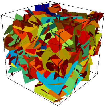
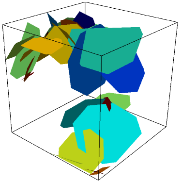
Figure 1: (a) A DFN composed of 499 fractures. (b) Backbone extracted from (a) using particles trajectories where a majority of mass transport occurs. Inlet plane is shown on front left; outlet plane is on rear right.

3 Graph Representation

3.1 Graph Formation

We construct a graph representation of each DFN based on the network topology using the method described in Hyman, et al. hyman2017accurate . For every fracture in the DFN, there is a unique node in a graph. If two fractures intersect, then there is an edge in the graph connecting the corresponding nodes. This mapping between DFN and graph naturally assigns fracture-based properties, both geometric and hydrological, as node attributes. Edges are assigned unit weight to isolate topological attributes from other attributes that could be considered.

Source and target nodes are included into the graph to incorporate flow direction. Every fracture that intersects the inlet plane is connected to the source node and every fracture that intersects to the outlet plane is connected to the target node. The inclusion of flow direction is essential to identify possible transport locations, which depend upon the imposed pressure gradient neuman2005trends . An example of this mapping for a three-dimensional twelve fracture network is shown in figure 2. Each of the fractures (semi-transparent colored planes) are represented as nodes (black), intersections between fractures are represented by edges in the graph (solid black lines). The source node is colored blue and the target node is colored red.

Every subgraph has a unique pre-image in the fracture network that is a subnetwork of the full network because the mapping between the network and graph is bijective. Thus, flow and transport simulations can be performed on these subnetworks, and compared to results obtained on the full networks.

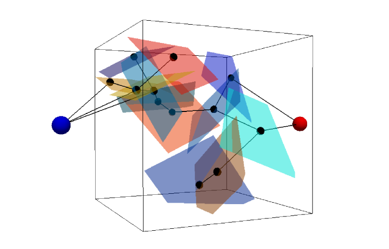
Figure 2: Graph representation of a twelve-fracture discrete fracture network in three dimensions. Fractures (semi-transparent colored planes) are represented as nodes (black), intersections between fractures are represented by edges in the graph (solid black lines). A source node (blue) and a target node (red) are also included into the graph to include boundary conditions and flow direction.

3.2 Node features

The centrality of a node in a graph describes its importance to transport across the network. Motivated by recent studies suggesting centrality measures that can help identify regions important in conducting flow and tansport Santiago2014 ; Santiago2016 , we consider four such quantities as node features. Three are global topological measures, quantifying how frequently paths through the graph include a given node. One is a local topological measure, giving the number of immediate neighbors of a node. Graph properties are computed using the NetworkX graph software package hagberg-2008-exploring . The topological features are supplemented with two physical (geometric) features; fracture volume projected along the main flow axis (from inlet plane to outlet plane) and fracture permeability. Figure 3 provides a visualization of a graph derived from the random DFN shown in Figure 1. Blue circles represent normalized feature values using these six different features, in panels a) through f). The yellow square and circle denote the source and target. Heavy lines represent particle backbone paths in the graphs.

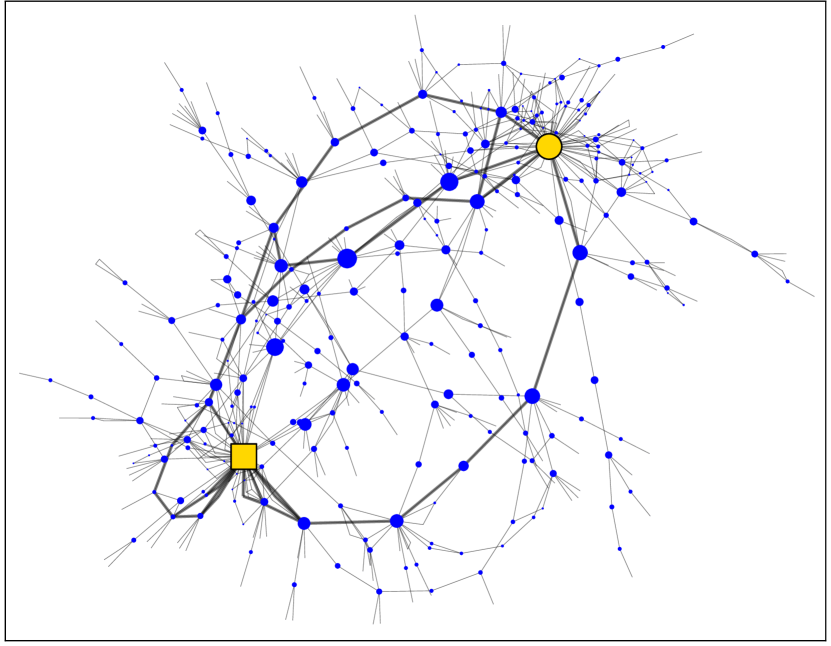
a) Betweenness centrality

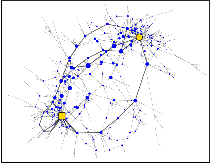
b) Source-to-target current flow

c) Source-to-target simple paths

d) Degree centrality

e) Projected volume

f) Permeability

Figure 3: Visualization of a graph derived from a random DFN as shown in Figure 1. Blue circles represent normalized feature values using six different features, in panels a) through f). Yellow square denotes source, yellow circle denotes target. Heavy lines represent particle backbone paths in the graphs. Note varying extent of correlation between particle backbone and associated feature strength.

3.2.1 Global topological features

• The betweenness centrality Anthonisse1971 ; Freeman1977 of a node (Figure 3a) reflects the extent to which that node can control communication on a network. Consider a geodesic path (path with fewest possible edges) connecting a node $u$ and a node $v$ on a graph. In general, there may be more than one such path: let $\sigma_{uv}$ denote the number of them. Furthermore, let $\sigma_{uv}(i)$ denote the number of such paths that pass through node $i$. We then define, for node $i$,

  $$\text{Betweenness centrality}=\frac{1}{(n-1)(n-2)}\sum_{\begin{subarray}{c}u,v=1\\ u\neq i\neq v\end{subarray}}^{n}\frac{\sigma_{uv}(i)}{\sigma_{uv}},$$ (1)

  where the leading factor normalizes the quantity so that it can be compared across graphs of different sizes $n$. Figure 3a confirms that many backbone nodes do indeed have high betweenness values. At the same time, certain paths through the network that are not part of the backbone also show high values for this feature, reflecting that betweenness centrality considers all paths in the graphs, and not only those from source to target.

• Source-to-target current flow (Figure 3b) is a centrality measure based on an electrical current model Brandes2005 , and assumes a given source and target. Imagine that one unit of current is injected into the network at the source, one unit is extracted at the target, and every edge has unit resistance. Then, the current-flow centrality at a node is equal to the current passing through it. This is given by Kirchhoff’s laws, or alternatively in terms of the graph Laplacian matrix $\mathbf{L}=\mathbf{D}-\mathbf{A}$, where $\mathbf{A}$ is the adjacency matrix for the graph and $\mathbf{D}$ is a (diagonal) matrix specifying node degree: $D_{ii}=\sum_{j}A_{ij}$. Letting $\mathbf{L}^{+}$ denote the Moore-Penrose pseudoinverse of $\mathbf{L}$, $s$ the source node, and $t$ the target node, then for node $i$ we define

  $$\text{Current flow }=\sum_{j=1}^{n}A_{ij}\bigl{|}\bigl{(}L_{is}^{+}-L_{js}^{+}\bigr{)}-\bigl{(}L_{it}^{+}-L_{jt}^{+}\bigr{)}\bigr{|}.$$ (2)

  Current-flow centrality is also known as random-walk centrality Newman2005 , since the same quantity measures how often a random walk from $s$ to $t$ passes through $i$. Unlike betweenness centrality, the current-flow centrality is zero on any branch of the graph outside of the central core. We therefore expect high current flow values to correlate with nodes that have large influence on source-to-target transport.

• Source-to-target simple paths (Figure 3c) is a centrality measure that counts simple (non-backtracking) paths crossing the graph from source $s$ to target $t$. Let $\pi_{st}$ denote the number of such paths, and $\pi_{st}(i)$ denote the number of those passing through node $i$. We then define, for node $i$,

  $$\text{Simple paths}=\frac{\pi_{st}(i)}{\pi_{st}},$$ (3)

  where normalization by $\pi_{st}$ allows comparing values of simple path centrality across different graphs. Due to the exponential proliferation of possible paths, we limit our search to paths with 15 nodes or less. Beyond 15, the effect on source-to-target simple path centrality is negligible. Figure 3c illustrates that nodes with high simple path centrality are more likely to lie on backbone paths than are nodes with high betweenness centrality in Figure 3a. However, simple path centrality also fails to identify one isolated backbone path that is disjoint from the others.

3.2.2 Local topological feature

• Degree centrality (Figure 3d) is a normalized measure of the number of edges touching a node. For node $i$,

  $$\text{Degree centrality}=\frac{1}{n-1}\sum_{j=1}^{n}A_{ij}.$$ (4)

  Nodes with high degree centrality tend to be concentrated in the core of the network. Conversely, nodes with low degree centrality are often in the periphery or on branches that cannot possibly conduct significant flow and transport. Physically, degree centrality of a fracture measures the number of other fractures that intersect with it.

3.2.3 Physical features

We supplement the four topological features with two features describing physical properties of fractures.

• Projected volume (Figure 3e) measures the component of a fracture’s volume oriented along the direction of flow from inlet to outlet plane. Let fracture $i$ have volume $V_{i}$ and orientation vector $\mathbf{O}_{i}$ (unit vector normal to the fracture plane). Taking flow to be oriented along the $x$-axis, the projected volume is expressed by the projection of $\mathbf{O}_{i}$ onto the $yz$-plane:

  $$\text{Projected volume}=V_{i}\sqrt{(O_{i})_{y}^{2}+(O_{i})_{z}^{2}}.$$ (5)

  Figure 3e shows similarities between this feature and degree centrality, but also some fractures where one feature correlates more closely with the backbone than the other.

• Permeability (Figure 3f) measures how easily a porous medium allows flow to pass therein. Given the aperture size $b_{i}$ of fracture $i$, the permeability is expressed as

  $$\text{Permeability}=\frac{b_{i}^{2}}{12}$$ (6)

  The permeability of a fracture, which is nonlinearly related to its volume, is a measure of its transport capacity. As illustrated in Figure 3, it displays similarities to both degree centrality and projected volume, with backbone fractures almost systematically having high permeability values (but the converse holding less consistently).

3.3 Correlation of feature values

Figure 4: Heat map displaying correlations among the particle backbone and the six features used.

As is seen in Figure 3, the feature values vary widely from one node to another, in ways that we aim to manipulate in order to generate subnetworks. Figure 4 shows correlation coefficients for pairs that include the particle backbone and the six features that we have chosen. That there are non-negligible correlations between the backbone and these features suggests that they are relevant ones for classification, although clearly no single feature is sufficient in itself. The correlation coefficients indicate that features tend to cluster naturally into the three categories above. The first three features, which are the global topological ones (betweenness, current flow, and simple paths), have significant mutual correlations among then. The same is true for the physical features (projected volume and permeability), which also exhibit some clustering with the related local topological feature (degree centrality). The latter correlations are consistent with our feature definitions above.

While we also considered additional centrality measures studied in the literature Santiago2014 ; Santiago2016 , such as closeness, eccentricity, and eigenvector centrality, we found that those exhibited much weaker correlations with the particle backbone. The choice of the six features above was motivated through cross-validation tests, where adding centrality measures did not improve classification performance while removing any of them degraded performance.

4 Classification Methods

In this section, we explain how we evaluate classification performance, briefly describe our two machine learning algorithms (random forest and support vector machines), and our process for parameter selection. Detailed descriptions of the methods are provided in the appendix. Both algorithms are general-purpose supervised learning methods suitable for geometric as well as non-geometric features. Given a set of features and class assignment for some observations, supervised learning algorithms try to “learn” the underlying function that maps features to classes. Those observations are the training set. Once learned, the function can then be used to classify new observations. In our study, we use as observations the nodes (fractures) from 80 graphs as a training set. We then test the function using nodes from 20 graphs as a test set. Both algorithms are implemented using the scikit-learn machine learning package in python, with the functions RandomForestClassifier and SVC.

4.1 Performance measures

There are a number of challenges in evaluating classification performance. Our problem has a large class imbalance: only about 7 percent of nodes in the training set are in the particle backbone. A classifier could simply assign all nodes to the non-backbone class, and still achieve an overall accuracy of 93 percent. Moreover, our approach departs from more conventional machine learning methodology in that our ultimate objective is not necessarily a perfect recovery of the backbone. We train on the particle backbone in order to identify a subset of fractures that share its characteristics, thereby reducing the full network to a subnetwork with analogous flow behavior. We then validate the flow behavior using the breakthrough curve (BTC), which describes the distribution of times for particles to pass through the network. For these reasons, performance measures must be interpreted with care.

For straightforward backbone prediction, we may define a positive classification of a node as being an assignment to the backbone class, and a negative classification as being an assignment to the non-backbone class. True positives (TP) and true negatives (TN) represent nodes whose backbone/non-backbone assignment matches that of the labeled data. False positives (FP) and false negatives (FN) represent nodes whose backbone/non-backbone assignment is opposite that of the labeled data. One measure of success is the TP rate. Precision ($p$) and recall ($r$) represent two kinds of TP rates:

$$p=\frac{TP}{TP+FP}$$ (7)

$$r=\frac{TP}{TP+FN}$$ (8)

Precision is the number of true positives over the total number that we classify as positive, whereas recall is the number of true positives over the total number of actual positives. These values give an understanding of how reliable (precision) and complete (recall) our results are.

Figure 5: Precision/recall curve for current-flow thresholding as a classifier. As threshold value increase, classifier moves from perfect recall to perfect precision. Ideally, precision/recall curve would touch upper-right corner for strongest classifier performance.

There is a tradeoff between precision and recall. This can be seen in the behavior of one of the simplest possible forms of classification: thresholding according to a single feature. Consider a classifier that labels as backbone all fractures with nonzero current flow. The process would resemble the dead-end fracture chain removal method common in the hydrology literature, but more extreme in that it would eliminate all dead-end subnetworks. This gives perfect (100%) recall, since all fractures in the particle backbone necessarily have nonzero current flow, and 15% precision, as it reduces the network to approximately half of its original size (about 7% of which were TP). Now imagine increasing the threshold, so as to lower the number of positive assignments. This will reduce FP, thereby increasing the precision. However, it will also increase FN, reducing the recall. In this way, we can travel along a precision/recall curve, shown in Figure 5, that has perfect recall as one extreme and perfect precision as the other. If there existed a threshold value at which the classifier recovered the class labels perfectly, the precision/recall curve would touch the upper-right corner of the figure: 100% precision and 100% recall. One typically wants classifiers that come as close to that ideal as possible.

In order to quantify the tradeoff shown in Figure 5, one may introduce a utility function

$$u_{\alpha}({\mathbf{q}})=\alpha p({\mathbf{q}})+(1-\alpha)r({\mathbf{q}}),$$ (9)

where $\alpha\in[0,1]$ specifies the relative weight of precision vs. recall, $\mathbf{q}$ denotes a vector of hyperparameter values used for tuning the classifier, and $p({\mathbf{q}})$ and $r({\mathbf{q}})$ denote the precision and recall obtained by the classifier for those parameter values. Thus, $u_{\alpha}({\mathbf{q}})$ is determined purely by recall when $\alpha=0$, and purely by precision when $\alpha=1$. In the example above, ${\mathbf{q}}$ would be a scalar quantity $q$ denoting the current-flow threshold value. In general, for a given weight $\alpha$, we may find the hyperparameter values $\mathbf{q}$ that maximize $u_{\alpha}({\mathbf{q}})$. The most straightforward algorithm for doing so is grid search cross-validation, which performs an exhaustive search over a given range of $\mathbf{q}$ values, evaluating $p({\mathbf{q}})$ and $r({\mathbf{q}})$ based on subsampling of the training data. This procedure avoids overfitting that would occur from validation using only the test data.

While the tradeoff between precision and recall is related to the tradeoff between network reduction and accuracy, it is not identical. Network reduction is measured by the ratio

$$\text{Fractures remaining}=\frac{TP+FP}{n}=\frac{r}{p}\,\frac{TP+FN}{n}=\frac{r}{p}\,\beta,$$ (10)

where $n$ is the number of fractures in the full network and $\beta$ is the proportion of fractures that are in the particle backbone. Low recall and high precision therefore yield small subnetworks. Accuracy is measured by the agreement between the BTC of the subnetwork and of the full network. High accuracy correlates with high recall: we train our classifier on the particle backbone because it is a valid network reduction from the perspective of characterizing where the majority of flow, and thus transport, occurs. But it is only one of many valid reductions. Ideally, one could optimize accuracy by computing the BTC for the subnetwork predicted with each choice of hyperparameters $\mathbf{q}$ in our grid search, and comparing with the full network’s BTC. Unfortunately, such a framework is computationally infeasible, since meshing a DFN, solving for flow and transport requires tens of minutes of wall clock time for each set of $\mathbf{q}$ values. Consequently, in place of high accuracy, we aim for high (though not necessarily perfect) recall. Precision is less essential: false positives increase the size of the predicted subnetwork, but for a small backbone ($\beta\approx 0.07$), even low precision allows for significant network reduction.

4.2 Random forest

A random forest ho_rf_1995 ; ho_rf_1998 is constructed by sampling from the training set with replacement, so that some data points may be sampled multiple times and others not at all. Those data points that are sampled are used to generate a large collection of decision trees, each of which outputs a classification based on feature values. Those data points that are not sampled are run through the decisions trees. A test data point is then classified by having each tree “vote” on its class. This leads not only to a predicted classification, but also to a measure of certainty (the fraction of trees that voted for it) as well as to an estimate of the importance of each feature for the class assignment Breiman2001 . That final estimate is particularly useful when the features consist of quantities that measure different aspects of node centrality. Further discussion of the random forest method is provided in the appendix.

In order to identify the hyperparameters of random forest that affect our results most significantly, we use the grid search cross-validation method described above, implemented with the GridSearchCV function in scikit-learn. We aim for high recall (low $\alpha$, in Eq. (9)), and find the greatest sensitivity to a hyperparameter that sets the minimal number of samples in a leaf node, to limit how much a decision tree branches. This is the sole hyperparameter for our classifier, so the vector ${\mathbf{q}}$ in Eq. (9) reduces to a scalar quantity $q$. Adjusting its value prevents overfitting, which in the context of unbalanced classes could cause practically none of the feature space to be assigned to the minority class Chen2004 .

4.3 Support vector machines

Support vector machines (SVM) separate high-dimensional data points into two classes by finding an appropriate hyperplane. Based on the generalized portrait algorithm Vapnik1963 and subsequent developments in statistical learning theory Vapnik1974 , the current version of SVM cortes_svm_1995 uses kernel methods Boser1992 to generalize linear classifiers to nonlinear ones. These are discussed further in the appendix. Kernel methods enable SVM to perform well when certain feature variables are highly correlated or even unimportant to the class assignment James2013 , and help prevent overfitting. We therefore enlarge our feature space for SVM by ranking the values of each feature on the nodes of a given graph. For a given feature, if $n$ nodes have feature values $f_{1},\dots,f_{n}$, then we define ranked features $\hat{f}_{1},\dots,\hat{f}_{n}$ whose values are given by the order statistics of $f$, i.e.,

$$\hat{f}_{i}=1 f_{i}=\min\{f_{1},\dots,f_{n}\},$$ if (11)

$$\hat{f}_{i}=n f_{i}=\max\{f_{1},\dots,f_{n}\},$$ if (12)

and generally, the ranked feature $\hat{f}_{i}=k$ if the “raw” feature $f_{i}$ is equal to the $k$th order statistic $f_{(k)}$. We supplement the collection of six raw features discussed in Section 3.2 with the six corresponding ranked features, resulting in a total of twelve features.

As with random forest, we use grid search cross-validation to identify and optimize crucial hyperparameters in SVM. We find the most important of these to be the penalty parameter, a regularization coefficient that controls the strictness of the decision boundary. When the penalty is large, SVM imposes a hard (rough) boundary in the training data, at the risk of overfitting. When the penalty is small, SVM allows a smoother boundary and more misclassification among the training data. Because of our class imbalance, we assign different penalty values for each class, so that the classifier more strictly bounds the (minority) backbone nodes than the (majority) non-backbone nodes Osuna1997 . These quantities form the two hyperparameters ($\mathbf{q}$ in Eq. 9) for our classifier. In this way, we can simultaneously prevent overfitting the majority class and “overlooking” points in the minority class. By adjusting the balance of penalty values, we control how likely the classifier is to assign a node to the backbone.

5 Results

We used a collection of 100 graphs. 80 were chosen as training data, and 20 were chosen as test data. We illustrate certain results, including breakthrough curves, on the DFN shown in Figure 1. Other results are based on the entire test set, which consists of a total of 9238 fractures, 651 of which (7.0%) are in the particle backbone and 8587 of which (93%) are not. The total computation time to train both RF and SVM was on the order of a minute, negligible compared to the time to extract the particle backbone needed for training. Once trained, the classifier ran on each test graph in seconds.

5.1 Classifiers

Classifier	Precision	Recall	Fractures remaining
RF(1400)	18%	90%	36%
RF(30)	26%	75%	21%
RF(15)	30%	65%	15%
RF(1)	58%	20%	2.5%

Table 1: Random forest classifiers labeled by the min_samples_leaf parameter value, controlling how much a decision tree can branch. Percentages for precision, recall, and fractures remaining in network are calculated over all 20 graphs in the test set.

We implemented random forest using the RandomForestClassifier function in scikit-learn, on the six features described in Section 3.2. Based on cross-validation with the function GridSearchCV, we found default hyperparameter values to be sufficient for achieving high recall, except as follows: 250 trees (n_estimators=250); best split determined by binary logarithm of number of features (max_features=log2); information gain as the quality measure for a split (criterion=‘entropy’); voting weights inversely proportional to class frequency (class_weight=‘balanced_subsample’). We varied the minimal number of training samples in a leaf node (min_samples_leaf) to adjust the tradeoff between recall and precision. Table 1 shows the results for a sample of four different hyperparameter values; one can also explicitly find the value that maximizes the utility function $u_{\alpha}(q)$ for a sample of different $\alpha$ values, using GridSearchCV. Since the full particle backbone accounts for only 7% of the fractures in the test set, we see that even classifiers with relatively low precision can reduce the network significantly.

Random forest also provides a quantitative estimate of the relative importance of each of the six features described in Section 3.2, based on how often a tree votes for it. Using the RF(30) model on our 80 training graphs, we find the feature importances shown in Figure 6. The source-to-target current flow, source-to-target simple paths, and betweenness centralities are the most important features, followed by node degree, and followed finally by permeability and projected volume. Thus, as with the feature correlations shown in Figure 4, the feature importances cluster into three natural groups. Global topological features have the greatest importance, local topological features have significant but lower importance, and physical features play only a small role in classification. In contrast with SVM, the performance of random forest does not benefit from using additional features such as ranked features. The inherent bootstrapping of random forest enables strong classification performance even with a relatively limited number of features.

Figure 6: Relative importances of features based on training data for random forest.

We implemented SVM using the SVC function in scikit-learn, on the twelve features made up of the six raw features described in Section 3.2 along with their ranked counterparts. We chose penalty value pairs (class_weight, often called $C$ in the literature cortes_svm_1995 ; Osuna1997 ) for the backbone and non-backbone class, which we adjusted in order to vary precision and recall. Table 2 shows results for a sample of four different pairs of values. Similarly to RF, one could find value pairs ${\mathbf{q}}$ that maximize the utility function $u_{\alpha}({\mathbf{q}})$ for a sample of different $\alpha$ values, by using the GridSearchCV cross-validation function. All other parameters were set to their default values, which include a radial kernel (closed decision boundary).

Classifier	Precision	Recall	Fractures remaining
SVM(0.90,0.054)	17%	96%	39%
SVM(0.90,0.063)	19%	90%	34%
SVM(0.70,0.070)	23%	78%	24%
SVM(0.70,0.190)	44%	46%	7.3%

Table 2: SVM classifiers labeled by the class_weight parameter pair values, specifying misclassification penalties for the backbone and non-backbone classes. Percentages for precision, recall, and fractures remaining in network are calculated over all 20 graphs in the test set.

5.2 Validation

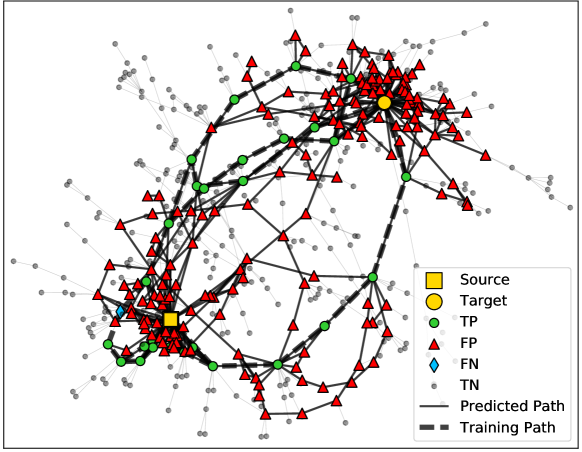
(a) (b)

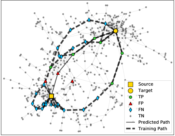
Figure 7: Extreme cases of classification results: (a) SVM(0.90,0.054) with high recall and low precision (40% of network remaining), showing many false positives (FP) and relatively few false negatives (FN), and (b) RF(1) with low recall and high precision (2% of network remaining), showing many false negatives (FN) and relatively few false positives (FP). Solid lines show predicted paths from source to target. Dashed lines show particle backbones.

In order to evaluate the quality of our classification results, we illustrate two cases on the DFN from Figure 1. In Figure 7 (a), we visualize the result of our classifier with the highest recall and lowest precision, SVM(0.90,0.054). Most of the nodes in the particle backbone are classified as positive. The few false negatives (FN) are near the source, and are primarily fractures intersecting the source plane where high particle concentrations accumulate. False positives (FP) are far more prevalent, forming many connected source-to-target paths that are not in the particle backbone. In spite of these, the reduced network identified by the classifier contains only 40% of the original fractures.

In Figure 7 (b), we visualize the result of our classifier with the highest precision and lowest recall, RF(1). While we see almost no false positives (FP), most of the nodes in the particle backbone are missed. The false negatives (FN) near the source are not necessarily of great concern, as these simply represent the inlet plane, but only one connected path exists between source and target. On some other networks in the test set, the classifier does not even generate a connected source-to-target path at all. The drastic reduction of network size, to 2% of the original fractures, results in too much loss of physical relevance.

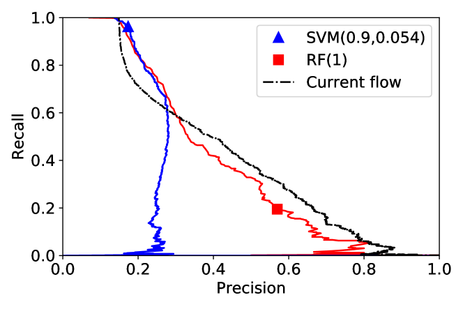
Figure 8: Precision/recall obtainable with one SVM and one RF classifier, along with current-flow thresholding for comparison. Markers indicate performance of unmodified classifier.

It is instructive to consider the full range of accessible precision and recall values for the classifiers above, as we did for the simple current-flow thresholding method in Section 4. Given a trained classifier with given hyperparameter values $\mathbf{q}$, one can modify it to give more or fewer positive assignments, effectively changing the percentage of votes needed for a positive classification (in the case of RF) or shifting the decision boundary (in the case of SVM). Note that this is not the same as generating different classifiers from the training data, as in Tables 1 and 2. Figure 8 shows precision/recall curves generated in this way for the two classifiers used in Figure 7, along with the current-flow curve as a baseline comparison. Marker values represent the precision/recall values seen in Tables 1 and 2 for the unmodified classifiers. It appears at first that current-flow thresholding has the strongest performance below about 60% recall. However, as with RF(1) above, these are nonphysical results: it generates connected subnetworks only for the highest recall values, where it significantly underperforms RF and SVM.

As discussed earlier, our primary objective is not reconstructing training data, but rather reducing network size while maintaining crucial flow properties. These properties are measured by the breakthrough curve (BTC), which gives the distribution of simulated particles passing through the network from source plane to target plane in a given interval of time. This is a common quantity of interest in subsurface systems, where one needs to predict the travel time distribution through the fracture network in order to evaluate the performance of systems such as hydraulic fracturing, nuclear waste disposal or gas migration from a nuclear test. We would like the BTC for our reduced networks to match that of the full network in a number of respects, notably the shape of the cumulative distribution function and the fraction of particles that reach the target plane after a given time.

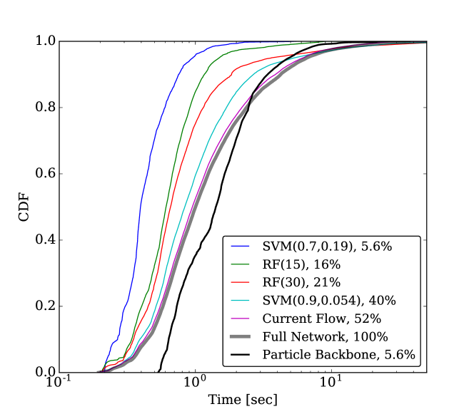
Figure 9: Predictions for the DFN from Figure 1, visualized as BTC (cumulative distribution function) produced by dfnWorks. Representative results from four models are given, together with current-flow thresholding, full network and particle backbone. Legend shows model parameters and size of reduced network.

Figure 9 shows the BTC on this network for a representative sample of four of our classifiers. As a comparison, we also show the BTC for thresholding on nonzero current flow, as well as for the full network and for the particle backbone. While current flow thresholding gives a very close match, it only reduces the network to 52% of its original size. SVM(0.9,0.054) and RF(30) reduce the network to 40% and 21%, while still providing acceptable matches. The median breakthrough time for RF(30) deviates from that of the full network by approximately the same amount as the particle backbone, though in the opposite direction: it underestimates rather than overestimates the breakthrough time.

Finally, in order to quantify the tradeoff between BTC agreement and network reduction, we calculate the Kolmogorov-Smirnov (KS) statistic, giving a measure of “distance” between two probability distributions. The KS statistic is independent of binning, and most sensitive to discrepancies close to the medians of the distributions, making it particularly suitable for comparing BTCs. The results are summarized in Table 3. They confirm that the classifier with highest recall, SVM(0.90,0.054), which reduces the network to 40% of its original size, has a BTC close to that of the full network (KS statistic 0.10).

Classifier	Fractures remaining	KS
Current flow	52%	0.03
SVM(0.90,0.054)	40%	0.10
RF(1400)	38%	0.12
SVM(0.90,0.063)	35%	0.12
SVM(0.70,0.070)	22%	0.25
RF(30)	21%	0.26
RF(15)	16%	0.35
SVM(0.70,0.190)	5.6%	0.59
RF(1)	2.0%	0.68

Table 3: Results of applying current-flow thresholding, four RF and four SVM models to the DFN from Figure 1. Fractures remaining in network are those identified as positive by classifier. Values differ slightly from results over entire test set, due to graph-to-graph fluctuations. KS statistic represents distance between breakthrough curve on reduced network and on full network.

6 Discussion and Conclusions

We have presented a novel approach to finding a high-flow subnetwork that does not require resolving flow in the network, and that takes minimal computational time. The method involves representing a DFN as a graph whose nodes represent fractures, and applying machine learning techniques to rapidly predict which nodes are part of the subnetwork. We used two supervised learning techniques: random forest and support vector machines. Once these algorithms have been trained on flow data from particle simulations, they successfully reduce new DFNs while preserving crucial flow properties. Our algorithms use topological features associated with nodes on the graph, as well as a small number of physical features describing a fracture’s properties. We consider each node as a point in the multi-dimensional feature space, and classify it according to whether or not it belongs to the subnetwork.

By varying at most two parameters of our classifiers, we are able to obtain a wide range of precision and recall values. These yield subnetworks whose sizes range from 40% down to 2% of the original network. For reductions to as little as 21% of the original size, the resulting breakthrough curve (BTC) displays good agreement with that of the original network. We therefore obtain significantly reduced networks that are useful for flow and transport simulations and generated in seconds. By comparison, the computation time needed to extract the particle backbone is on the order of an hour. We use cross-validation to identify the crucial classifier parameters, and show how to use it to tune these parameters, optimizing precision for fixed recall or vice-versa. To the extent that recall approximates BTC agreement, this can result in maximal network reduction for a given level of accuracy, or maximal accuracy for a given level of network reduction.

In addition to the classification results, the random forest method gives a set of relative importances for the features used. These importances are determined by permuting the values of a given feature and observing the effect this has on classification performance. We have found that features based on global topological properties of the underlying graph were significantly more important than those based on geometry or physical properties of the fractures. This reinforces previous observations that network connectivity is more fundamental to determining where flow occurs in a network than are geometric or hydraulic properties for sparse networks hyman2016fracture . Quantitatively, the most important of our global topological features is source-to-target current flow, which measures how much of a unit of current injected at the source (representing the inlet plane of the DFN) passes through a given node of the graph.

Indeed, classifying fractures only based on whether they conduct nonzero current flow yields in itself a reasonable graph reduction of around 50%, with a BTC that very closely matches the original network. However, this does not generalize to a method allowing arbitrary graph reduction: raising the current-flow threshold above zero reduces the number of fractures, but results in subnetworks that are disconnected and therefore nonphysical. By contrast, when we use the full set of classification features, we consistently realize a connected subnetwork for all but the lowest recall values. It is somewhat remarkable that this occurs in spite of our classifiers never explicitly making use of source-to-target paths in the graph.

In principle, the performance of classifiers in this framework depends on the particular geometric and hydrological properties of the fracture network generation parameters and the inferred topological structures. Changing generation parameters will not only result in different geometries, but also different topological properties of the network realizations. Depending on the prescribed distributions of fracture radii, network density, fracture shape, fracture intensity, etc., what features should be considered in the classifier might also change. Thus, it is imperative that the classifiers must be trained using the particular ensemble in which they want to predict the subnetworks.

Finally, some evidence suggests that if one could in fact classify paths rather than nodes, results would improve further. We are currently exploring a classification method that initially labels fractures at the inlet and outlet planes, and then successively attempts to propagate positive identifications through the network, thereby forming source-to-target paths. The objective of this method is to generate subnetworks that are far closer to the particle backbone itself. Thus, the training data would be used not merely to guide the classifier toward useful network reductions, but rather in the more conventional machine learning setting of providing ground truth to be reproduced. Preliminary tests suggest that such a method may considerably boost precision and recall simultaneously, generating subnetworks whose BTC closely matches the full network but whose size is not much larger than the particle backbone.

7 Acknowledgments

The authors are grateful to an anonymous reviewer, for comments and suggestions that helped improve the clarity and readability of the manuscript. This work was supported by the Computational Science Research Center at San Diego State University, the National Science Foundation Graduate Research Fellowship Program under Grant No. 1321850, and the U.S. Department of Energy at Los Alamos National Laboratory under Contract No. DE-AC52-06NA25396 through the Laboratory Directed Research and Development program. JDH thanks the LANL LDRD Director’s Postdoctoral Fellowship Grant $\#$ 20150763PRD4 for partial support. JDH, HSV, and GS thank LANL LDRD-DR Grant $\#$20170103DR for support.

Flow Equations and transport simulations

We assume that the matrix surrounding the fractures is impermeable and there is no interaction between flow within the fractures and the solid matrix. Within each fracture, flow is modeled using the Darcy flow. The aperture within each fracture is uniform and isotropic, but they do vary between fractures and are positively correlated to the fracture size hyman2016fracture . Locally, we adopt the cubic law witherspoon1980validity to relate the permeability of each fracture to its aperture. We drive flow through the domain by applying a pressure difference of 1MPa across the domain aligned with the x-axis. No flow boundary conditions are applied along lateral boundaries and gravity is not included in these simulations. These boundary conditions along with mass conservation and Darcy’s law are used to form an elliptic partial differential equation for steady-state distribution of pressure within each network

$$\nabla\cdot(k\nabla P)=0\leavevmode\nobreak\ .$$ (13)

Once the distribution of pressure and volumetric flow rates are determined by numerically integrating (13) the methodology of Makedonska et al. makedonska2015particle and Painter et al. painter2012pathline and are used to determine the Eulerian velocity field ${\mathbf{u}}({\mathbf{x}})$ at every node in the conforming Delaunay triangulation throughout each network.

The spreading of a nonreactive conservative solute transported is represented by a cloud of passive tracer particles, i.e., using a Lagrangian approach. The imposed pressure gradient is aligned with the $x$-axis and thus the primary direction of flow is in the $x$ direction. Particles are released from locations in the inlet plane ${\mathbf{x}}_{0}$ at time $t=0$ and are followed until the exit the domain at the outlet plane ${\mathbf{x}}_{L}$ The trajectory ${\mathbf{x}}(t;{\mathbf{a}})$ of a particle starting at ${\mathbf{a}}$ on ${\mathbf{x}}_{0}$ is given by the advection equation, $\dot{{\mathbf{x}}(t;{\mathbf{a}})}={\mathbf{v}}(t;{\mathbf{a}})$ with ${\mathbf{x}}(0;{\mathbf{a}})={\mathbf{a}}$ where the Lagrangian velocity ${\mathbf{v}}(t;{\mathbf{a}})$ is given in terms of the Eulerian velocity ${\mathbf{u}}({\mathbf{a}})$ as ${\mathbf{v}}(t;\mathbf{{\mathbf{a}}})={\mathbf{u}}[{\mathbf{x}}(t;{\mathbf{a}})]$. The mass represented by each particle $m({\mathbf{a}})$ and the breakthrough time at the outlet plane, $\tau({\mathbf{x}}_{L};{\mathbf{a}})$ of a particle that has crossed the outlet plane, ${\mathbf{x}}_{L}=(L,y,z)$ is can be combined to compute the total solute mass flux $\psi(t)$ that has broken through at a time $t$,

$$\Psi(t,{\mathbf{x}}_{L})=\frac{1}{M}\int\limits_{\Omega_{a}}dm({\mathbf{a}})\delta[t-\tau({\mathbf{x}}_{L},{\mathbf{a}})]\leavevmode\nobreak\ ,$$ (14)

where $\Omega_{a}$ is the set of all particles. Here mass is distributed uniformly amongst particles, i.e., resident injection is adopted. For more details about the injection mode see Hyman et al., hyman2015influence .

Algorithm Description

Random Forest

The random forest method is based on constructing a collection of decision trees. A decision tree russell2010artificial is a tree whose interior nodes represent binary tests on a feature and whose leaves represent classifications. An effective way of constructing such a tree from training data is to measure how different tests, also called splits, separate the data. The information gain measure compares the entropy of the parent node to the weighted average entropy of the child nodes for each split. The splits with the greatest information gain are executed, and the procedure is repeated recursively for each child node until no more information is gained, or there are no more possible splits. A limitation of decision trees is that the topology is completely dependent on the training set. Variations in the training data can produce substantially different trees.

The random forest method ho_rf_1995 ; ho_rf_1998 addresses this problem by constructing a collection of trees using subsamples of the training data. These subsamples are generated with replacement (bootstrapping), so that some data points are sampled more than once and some not at all. The sampled “in-bag” data points are used to generate a decision tree. The “out-of-bag” observations (the ones not sampled) are then run through the tree to estimate its quality liaw_classification_2002 . This procedure is repeated to generate a large number (hundreds or thousands) of random trees.

To classify a test data point, each tree “votes” for a result. This provides not only a predicted classification, determined by majority rule, but also a measure of certainty, determined by the fraction of votes in favor. The use of bootstrapping effectively augments the data, allowing random forest to perform well using fewer features than other methods. The category with more votes is assigned to the new observation. The idea of random decision forests originated with T. Ho in 1995. Ho found that forests of trees partitioned with hyperplanes can have increased accuracy under certain conditions ho_rf_1995 . In a later work ho_rf_1998 , Ho determined that other splitting methods, under appropriate constraints, yielded similar results.

Additionally, random forest provides an estimate of how important each individual feature is for the class assignment. This is calculated by permuting the feature’s values, generating new trees, and measuring the “out-of-bag” classification errors on the new trees. If the feature is important for classification, these permutations will generate many errors. If the feature is not important, they will hardly affect the performance of the trees.

Support vector machines

Support vector machines (SVM) use a maximal margin classifier to perform binary classification. Given training data described by $p$ features, the method identifies boundary limits for each class in the $p$-dimensional feature space. These boundary limits, which are $(p-1)$-dimensional hyperplanes, are known as local classifiers, and the distance between the local classifiers is called the margin. SVM attempts to maximize this margin, making the data as separable as possible, and defines the classifier as a hyperplane in the middle that separates the data into two groups. The data points on the boundaries are called support vectors, since they “support” the limits and define the shape of the maximal margin classifier.

Formally, a support vector machine attempts to construct a hyperplane,

$$\langle{\bf a},{\bf x}_{i}\rangle+b=0\leavevmode\nobreak\ ,$$ (15)

that partitions data points ${\bf x}_{i}$ into disjoint sets, for $i\in\{1,\dots,n\}$. To define the hyperplane we must determine the unknown coefficients ${\bf a}=(a_{1},\ldots,a_{p})$ and $b$. SVM seeks to determine a hyperplane that separates the two sets $A$ and $B$ and leaves the largest margin.

Let $\langle{\bf a},{\bf x}_{i}\rangle+b=\pm 1$ be the normalized equations for the boundaries of the hyperplane margin. Data points ${\bf x}_{i}$ on either side of the margins of the hyperplane will lie in either $A$ and $B$ depending upon whether they satisfy either

$$\langle{\bf a},{\bf x}_{i}\rangle+b>1\qquad{\text{o}r}\qquad\langle{\bf a},{\bf x}_{i}\rangle+b<-1\leavevmode\nobreak\ .$$ (16)

Define an indicator function $S({\bf x})$ by

$$S({\bf x})=\begin{cases}1\qquad{\bf x}\in A\\ -1\qquad{\bf x}\in B\\ \end{cases}$$ (17)

and set $S_{i}=S({\bf x}_{i})$. Then we can combine (16) into a single inequality $(\langle{\bf a},{\bf x}_{i}\rangle+b)S_{i}\geq 1$ for all ${\bf x}_{i}$; with equality holding for support vectors, the nearest points to the margin.

In most cases the sets $A$ and $B$ may only be close to linearly separable. To account for this possibility we introduce slack variables $\xi_{i}\geq 0$,

$$(\langle{\bf a},{\bf x}_{i}\rangle+b)S_{i}\geq 1-\xi_{i}\qquad\forall\leavevmode\nobreak\ i\leavevmode\nobreak\ ,$$ (18)

that allows ${\bf x}_{i}$ corresponding to $\xi_{i}>0$ to be incorrectly classified with the $\xi_{i}$ being used as a penalty term. Distances $\rho_{1}$ and $\rho_{2}$ from the coordinate origin to the margin boundary are given by $\rho_{1}=-(b+1)/\|{\bf a}\|$ and $\rho_{2}=-(b-1)/\|{\bf a}\|$ where $\|{\bf a}\|$ is the Euclidean length of ${\bf a}$. The margin width is the distance between these two lines $d=\rho_{2}-\rho_{1}={2/\|{\bf a}\|}$. We seek to maximize $d$ or, equivalently, minimize $\|{\bf a}\|$, over the set of training data $({\bf y}_{1},\dots,{\bf y}_{m})$, subject to the linear constraints (18). Typically one works with the Lagrangian formulation of the constrained optimization problem. The dual Lagrangian problem is to minimize the objective function

$$L({\bf a},b,\boldsymbol{\xi},\gamma,\boldsymbol{\delta}) = \frac{1}{2}{\|{\bf a}\|}^{2}-\sum_{j=1}^{m}\gamma_{j}[(\langle{\bf a},{\bf y}_{j}\rangle+b)S_{j}-1+\xi_{j}]$$ (19)

$$+C\sum_{j=1}^{m}\xi_{j}-\sum_{j=1}^{m}\delta_{j}\xi_{j}\leavevmode\nobreak\$$

subject to the non-negativity constraints of the Lagrange multipliers $\gamma_{j},\delta_{j}$, and $\xi_{j}\geq 0$ and obtain ${\bf a}$ and $b$. The penalty, or margin parameter, $C$ is a regularization term that controls how many points are allowed to be mislabeled in the SVM hyperplane construction; smaller values of $C$ allow for more points to be mislabeled. A solution to this optimization problem defines ${\bf a}$ and $b$. The SVM classifier is then given by the sign of the decision function,

$$\chi({\bf x}_{i})=\operatorname{sgn}(\langle{\bf a},{\bf x}_{i}\rangle+b).$$ (20)

SVM falls into the category of kernel methods, a theoretically powerful and computationally efficient means of generalizing linear classifiers to nonlinear ones. For instance, on a two-dimensional surface ($p=2$ features), instead of the line described by equation (15), we can choose a polynomial curve or a radial loop. Equation (20) may then be written in the form

$$\chi({\bf x}_{i})=\operatorname{sgn}\left(\alpha_{0}+\sum_{j=1}^{m}\alpha_{j}K({\bf x}_{i},{\bf y}_{j})\right),$$ (21)

where $K({\bf x}_{i},{\bf y}_{j})$ is an appropriate kernel function of ${\bf x}_{i}$ and training point ${\bf y}_{j}$. Radial kernels often provide the best classification performance, but at higher computational costs.

References

- (1) Abelin, H., Birgersson, L., Moreno, L., Widén, H., Ågren, T., Neretnieks, I.: A large-scale flow and tracer experiment in granite: 2. results and interpretation. Water Resour. Res. 27(12), 3119–3135 (1991)
- (2) Abelin, H., Neretnieks, I., Tunbrant, S., Moreno, L.: Final report of the migration in a single fracture: experimental results and evaluation. Nat. Genossenschaft fd Lagerung Radioaktiver Abfälle (1985)
- (3) Aldrich, G., Hyman, J., Karra, S., Gable, C., Makedonska, N., Viswanathan, H., Woodring, J., Hamann, B.: Analysis and visualization of discrete fracture networks using a flow topology graph. IEEE T. Vis. Comput. Gr. (2016)
- (4) Andresen, C.A., Hansen, A., Le Goc, R., Davy, P., Hope, S.M.: Topology of fracture networks. Frontiers in Physics 1(August), 1–5 (2013). DOI 10.3389/fphy.2013.00007. URL http://www.frontiersin.org/Journal/10.3389/fphy.2013.00007/full
- (5) Anthonisse, J.: The rush in a directed graph. Stichting Mathematisch Centrum. Mathematische Besliskunde (BN 9/71), 1–10 (1971). URL http://www.narcis.nl/publication/RecordID/oai%3Acwi.nl%3A9791
- (6) Boser, B.E., Guyon, I.M., Vapnik, V.N.: A training algorithm for optimal margin classifiers. Proceedings of the fifth annual workshop on Computational learning theory COLT’92 p. 144 (1992). DOI 10.1145/130385.130401
- (7) Brandes, U., Fleischer, D.: Centrality measures based on current flow. Proc. 22nd Symp. Theoretical Aspects of Computer Science 3404, 533–544 (2005)
- (8) Breiman, L.: Random forests. Machine Learning 45(1), 5–32 (2001). DOI 10.1023/A:1010933404324
- (9) Chen, C., Liaw, A., Breiman, L.: Using random forest to learn imbalanced data. Tech. Rep. 666, University of California, Berkeley (2004)
- (10) Cortes, C., Vapnik, V.: Support-vector networks. Machine Learning 20(3), 273–297 (1995). DOI 10.1007/BF00994018
- (11) de Dreuzy, J.R., Méheust, Y., Pichot, G.: Influence of fracture scale heterogeneity on the flow properties of three-dimensional discrete fracture networks. J. Geophys. Res.-Sol. Ea. 117(B11) (2012)
- (12) Frampton, A., Cvetkovic, V.: Numerical and analytical modeling of advective travel times in realistic three-dimensional fracture networks. Water Resour. Res. 47(2) (2011)
- (13) Freeman, L.C.: A set of measures of centrality based on betweenness. Sociometry 40(1), 35–41 (1977)
- (14) Ghaffari, H.O., Nasseri, M.H.B., Young, R.P.: Fluid flow complexity in fracture networks: Analysis with graph theory and LBM. ArXiv e-prints p. 1107.4918 (2011)
- (15) Goetz, J.N., Brenning, A., Petschko, H., Leopold, P.: Evaluating machine learning and statistical prediction techniques for landslide susceptibility modeling. Computers and Geosciences 81, 1–11 (2015)
- (16) Hagberg, A.A., Schult, D.A., Swart, P.: Exploring network structure, dynamics, and function using networkx. In: Proceedings of the 7th Python in Science Conferences (SciPy 2008), vol. 2008, pp. 11–16 (2008)
- (17) Ho, T.K.: Random decision forests. Proceedings of the 3rd International Conference on Document Analysis and Recognition 14-16, 278–282 (1995)
- (18) Ho, T.K.: The random subspace method for constructing decision forests. IEEE Transactions on Pattern Analysis and Machine Intelligence 20(8), 832–844 (1998). DOI 10.1109/34.709601
- (19) Hope, S.M., Davy, P., Maillot, J., Le Goc, R., Hansen, A.: Topological impact of constrained fracture growth. Frontiers in Physics 3(September), 1–10 (2015). DOI 10.3389/fphy.2015.00075. URL http://journal.frontiersin.org/article/10.3389/fphy.2015.00075
- (20) Hyman, J., Jiménez-Martínez, J., Viswanathan, H., Carey, J., Porter, M., Rougier, E., Karra, S., Kang, Q., Frash, L., Chen, L., et al.: Understanding hydraulic fracturing: a multi-scale problem. Phil. Trans. R. Soc. A 374(2078), 20150,426 (2016)
- (21) Hyman, J.D., Aldrich, G., Viswanathan, H., Makedonska, N., Karra, S.: Fracture size and transmissivity correlations: Implications for transport simulations in sparse three-dimensional discrete fracture networks following a truncated power law distribution of fracture size. Water Resources Research 52(8), 6472–6489 (2016). DOI 10.1002/2016WR018806. URL http://dx.doi.org/10.1002/2016WR018806
- (22) Hyman, J.D., Gable, C.W., Painter, S.L., Makedonska, N.: Conforming Delaunay triangulation of stochastically generated three dimensional discrete fracture networks: A feature rejection algorithm for meshing strategy. SIAM J. Sci. Comput. 36(4), A1871–A1894 (2014)
- (23) Hyman, J.D., Hagberg, A., Srinivasan, G., Mohd-Yusof, J., Viswanathan, H.: Predictions of first passage times in sparse discrete fracture networks using graph-based reductions. Phys. Rev. E 96, 013,304 (2017). DOI 10.1103/PhysRevE.96.013304. URL https://link.aps.org/doi/10.1103/PhysRevE.96.013304
- (24) Hyman, J.D., Karra, S., Makedonska, N., Gable, C.W., Painter, S.L., Viswanathan, H.S.: dfnWorks: A discrete fracture network framework for modeling subsurface flow and transport. Computers and Geosciences 84, 10–19 (2015). DOI 10.1016/j.cageo.2015.08.001. URL http://dx.doi.org/10.1016/j.cageo.2015.08.001
- (25) Hyman, J.D., Painter, S.L., Viswanathan, H., Makedonska, N., Karra, S.: Influence of injection mode on transport properties in kilometer-scale three-dimensional discrete fracture networks. Water Resour. Res. 51(9), 7289–7308 (2015)
- (26) James, G., Witten, D., Hastie, T., Tibshirani, R.: An Introduction to Statistical Learning. Springer (2013)
- (27) Jenkins, C., Chadwick, A., Hovorka, S.D.: The state of the art in monitoring and verification—ten years on. Int. J. Greenh. Gas. Con. 40, 312–349 (2015)
- (28) Karra, S., Makedonska, N., Viswanathan, H., Painter, S., Hyman, J.: Effect of advective flow in fractures and matrix diffusion on natural gas production. Water Resources Research 51, 1–12 (2014)
- (29) LaGriT: Los Alamos Grid Toolbox, (LaGriT) Los Alamos National Laboratory. http://lagrit.lanl.gov (2013)
- (30) Liaw, A., Wiener, M.: Classification and regression by randomForest. R news 2(3), 18–22 (2002)
- (31) Lichtner, P., Hammond, G., Lu, C., Karra, S., Bisht, G., Andre, B., Mills, R., Kumar, J.: PFLOTRAN user manual: A massively parallel reactive flow and transport model for describing surface and subsurface processes. Tech. rep., (Report No.: LA-UR-15-20403) Los Alamos National Laboratory (2015)
- (32) Maillot, J., Davy, P., Le Goc, R., Darcel, C., De Dreuzy, J.R.: Connectivity, permeability, and channeling in randomly distributed and kinematically defined discrete fracture network models. Water Resources Research 52(11), 8526–8545 (2016)
- (33) Makedonska, N., Painter, S.L., Bui, Q.M., Gable, C.W., Karra, S.: Particle tracking approach for transport in three-dimensional discrete fracture networks. Computat. Geosci. pp. 1–15 (2015)
- (34) Mudunuru, M.K., Karra, S., Makedonska, N., Chen, T.: Joint geophysical and flow inversion to characterize fracture networks in subsurface systems. ArXiv e-prints p. 1606.04464 (2016)
- (35) National Research Council: Rock fractures and fluid flow: contemporary understanding and applications. National Academy Press (1996)
- (36) Neuman, S.: Trends, prospects and challenges in quantifying flow and transport through fractured rocks. Hydrogeol. J. 13(1), 124–147 (2005)
- (37) Newman, M.: A measure of betweenness centrality based on random walks. Social Networks pp. 39–54 (2005)
- (38) Osuna, E., Freund, R., Girosi, F.: Support vector machines: Training and applications. Tech. Rep. AIM-1602, Massachusetts Institute of Technology (1997)
- (39) Painter, S., Cvetkovic, V.: Upscaling discrete fracture network simulations: An alternative to continuum transport models. Water Resour. Res. 41, W02,002 (2005)
- (40) Painter, S., Cvetkovic, V., Selroos, J.O.: Power-law velocity distributions in fracture networks: Numerical evidence and implications for tracer transport. Geophys. Res. Lett. 29(14) (2002)
- (41) Painter, S.L., Gable, C.W., Kelkar, S.: Pathline tracing on fully unstructured control-volume grids. Computat. Geosci. 16(4), 1125–1134 (2012)
- (42) Rasmuson, A., Neretnieks, I.: Radionuclide transport in fast channels in crystalline rock. Water Resour. Res. 22(8), 1247–1256 (1986)
- (43) Robinson, B.A., Dash, Z.V., Srinivasan, G.: A particle tracking transport method for the simulation of resident and flux-averaged concentration of solute plumes in groundwater models. Computational Geosciences 14(4), 779–792 (2010)
- (44) Russell, S.: Artificial intelligence: a modern approach. Prentice Hall, Upper Saddle River, NJ (2010)
- (45) Santiago, E., Romero-Salcedo, M., Velasco-Hernández, J.X., Velasquillo, L.G., Hernández, J.A.: An integrated strategy for analyzing flow conductivity of fractures in a naturally fractured reservoir using a complex network metric. In: I. Batyrshin, M.G. Mendoza (eds.) Advances in Computational Intelligence: 11th Mexican International Conference on Artificial Intelligence, MICAI 2012, San Luis Potosí, Mexico, October 27 – November 4, 2012. Revised Selected Papers, Part II, pp. 350–361. Springer, Berlin, Heidelberg (2013)
- (46) Santiago, E., Velasco-Hernández, J.X., Romero-Salcedo, M.: A methodology for the characterization of flow conductivity through the identification of communities in samples of fractured rocks. Expert Systems With Applications 41(3), 811–820 (2014). DOI 10.1016/j.eswa.2013.08.011. URL http://dx.doi.org/10.1016/j.eswa.2013.08.011
- (47) Santiago, E., Velasco-Hernandez, J.X., Romero-Salcedo, M.: A descriptive study of fracture networks in rocks using complex network metrics. Computers and Geosciences 88, 97–114 (2016). DOI 10.1016/j.cageo.2015.12.021
- (48) Srinivasan, G., Tartakovsky, D.M., Dentz, M., Viswanathan, H., Berkowitz, B., Robinson, B.: Random walk particle tracking simulations of non-fickian transport in heterogeneous media. J. Comput. Phys. 229(11), 4304–4314 (2010)
- (49) Vapnik, V., Chervonenkis, A.Y.: Theory of pattern recognition: Statistical problems of learning [in russian] (1974)
- (50) Vapnik, V., Lerner, A.: Pattern recognition using generalized portrait method. Automation and Remote Control 24, 774–780 (1963)
- (51) Vevatne, J.N., Rimstad, E., Hope, S.M., Korsnes, R., Hansen, A.: Fracture networks in sea ice. Frontiers in Physics 2, 1–8 (2014). DOI 10.3389/fphy.2014.00021
- (52) Witherspoon, P.A., Wang, J., Iwai, K., Gale, J.: Validity of cubic law for fluid flow in a deformable rock fracture. Water Resour. Res. 16(6), 1016–1024 (1980)