Lifelong Generative Modeling

Abstract

Lifelong learning is the problem of learning multiple consecutive tasks in a sequential manner, where knowledge gained from previous tasks is retained and used to aid future learning over the lifetime of the learner. It is essential towards the development of intelligent machines that can adapt to their surroundings. In this work we focus on a lifelong learning approach to unsupervised generative modeling, where we continuously incorporate newly observed distributions into a learned model. We do so through a student-teacher Variational Autoencoder architecture which allows us to learn and preserve all the distributions seen so far, without the need to retain the past data nor the past models. Through the introduction of a novel cross-model regularizer, inspired by a Bayesian update rule, the student model leverages the information learned by the teacher, which acts as a probabilistic knowledge store. The regularizer reduces the effect of catastrophic interference that appears when we learn over sequences of distributions. We validate our model’s performance on sequential variants of MNIST, FashionMNIST, PermutedMNIST, SVHN and Celeb-A and demonstrate that our model mitigates the effects of catastrophic interference faced by neural networks in sequential learning scenarios. Our code is available at : https://github.com/jramapuram/LifelongVAE_pytorch.

1 Introduction

Machine learning is the process of approximating unknown functions through the observation of typically noisy data samples. Supervised learning approximates these functions by learning a mapping from inputs to a predefined set of outputs such as categorical class labels (classification) or continuous targets (regression). Unsupervised learning seeks to uncover structure and patterns from the input data without any supervision. Examples of this learning paradigm include density estimation and clustering methods. Both learning paradigms make assumptions that restrict the set of plausible solutions. These assumptions are referred to as hypothesis spaces, biases or priors and aid the model in favoring one solution over another [82, 128]. For example, the use of convolutions [70] to process images favors local structure; recurrent models [54, 46] exploit sequential dependencies and graph neural networks [109, 64] assume that the underlying data can be modeled accurately as a graph.

Current state of the art machine-learning models typically focus on learning a single model for a single task, such as image classification [72, 121, 43, 118, 66], image generation [100, 13, 63, 39], natural language question answering [25, 96] or single game playing [129, 113]. In contrast, humans experience a sequence of learning tasks over their lifetimes, and are able to leverage previous learning experiences to rapidly learn new tasks. Consider learning how to ride a motorbike after learning to ride a bicycle: the task is drastically simplified through the use of prior learning experience. Studies [2, 3, 67] in psychology have shown that humans are able to generalize to new concepts in a rapid manner, given only a handful of samples. [67] demonstrates that humans can classify and generate new concepts of two wheel vehicles given just a single related sample. This contrasts the state of the art machine learning models described above which use hundreds of thousands of samples and fail to generalize to slight variations of the original task [22].

Lifelong learning [126, 125] argues for the need to consider learning over task sequences, where learned task representations and models are stored over the entire lifetime of the learner and can be used to aid current and future learning. This form of learning allows for the transfer of previously learned models and representations and can reduce the sample complexity of the current learning problem [126]. In this work we restrict ourselves to a subset of the broad lifelong learning paradigm; rather than focus on the supervised lifelong learning scenario as most state of the art methods, our work is one of the first to tackle the more challenging problem of deep lifelong unsupervised learning. We also identity and relax crucial limitations of prior work in life-long learning that requires the storage of previous models and training data, allowing us to operate in a more realistic learning scenario.

2 Related Work

The idea of learning in a continual manner has been explored extensively in machine learning, seeded by the seminal works of lifelong-learning [126, 125, 117], online-learning [32, 9, 11, 12] and sequential linear gaussian models [105, 36] such as the Kalman Filter [56] and its non-linear counterpart, the Particle Filter [24]. Lifelong learning bears some similarities to online learning in that both learning paradigms observe data in a sequential manner. Online learning differs from lifelong learning in that the central objective of a typical online learner [11, 12] is to best solve/fit the current learning problem, without preserving previous learning. In contrast, lifelong learners seek to retain, and reuse, the learned behavior acquired over past tasks, and aim to maximize performance across all tasks. Consider the example of forecasting click through rate: the objective of the online learner is to evolve over time, such that it best represents current user preferences. This contrasts lifelong learners which enforce a constraint between tasks to ensure that previous learning is not lost.

Lifelong Learning [126] was initially proposed in a supervised learning framework for concept learning, where each task seeks to learn a particular concept/class using binary classification. The original framework used a task specific model, such as a K Nearest Neighbors (KNN) , coupled with a representation learning network that used training data from all past learning tasks (support sets), to learn a common, global representation. This supervised approach was later improved through the use of dynamic learning rates [115], core-sets [114] and multi-head classifiers [31]. In parallel, lifelong learning was extended to independent multi-task learning [107, 31], reinforcement learning [125, 122, 102], topic modeling [19, 130] and semi-supervised language learning [83, 81]. For a more detailed review see [20].

More recently, lifelong learning has seen a resurgence within the framework of deep learning. As mentioned earlier, one of the central tenets of lifelong learning is that that the learner should perform well over all observed tasks. Neural networks, and more generally, models that learn using stochastic gradient descent [103], typically cannot persist past task learning without directly preserving past models or data. This problem of catastrophic forgetting [78] is well known in the neural network community and is the central obstacle that needs to be resolved to build an effective neural lifelong learner. Catastrophic forgetting is the phenomenon where model parameters of a neural network trained in a sequential manner become biased towards the distribution of the latest observations, forgetting previously learned representations, over data no longer accessible for training. In order to mitigate catastrophic forgetting current research in lifelong learning employs four major strategies: transfer learning, replay mechanisms, parameter regularization and distribution regularization. In table 1 we classify the different lifelong learning methods that we will discuss in the following paragraphs into these strategies.

EWC [65] VCL [91] LwF [71] ALTM [33] PNN [94] DGR [112, 57] DBMNN [123] SI [136] VASE [1] LGM (us) Transfer learning ✗ ✗ ✗ ✗ ✓ ✗ ✓ ✗ ✗ ✗ Replay mechanisms ✗ ✓ ✗ ✗ ✗ ✓ ✗ ✗ ✓ ✓ Parameter regularization ✓ ✓ ✗ ✗ ✗ ✗ ✗ ✓ ✗ ✗ Functional regularization ✗ ✗ ✓ ✓ ✗ ✗ ✗ ✗ ✓ ✓

Table 1: Catastropic interference mitigation strategies of state of the art models. Rows highlighted in gray represent desirable mitigation strategies.

Transfer learning: These approaches mitigate catastrophic forgetting by freezing previous task models and relaying a latent representation of the previous task to the current model. Research in transfer learning for the mitigation of catastrophic forgetting include Progressive Neural Networks (PNN) [94] and Deep Block-Modular Neural Networks (DBMNN) [123] to name a few. These approaches allow the current model to adapt its parameters to the (new) joint representation in an efficient manner and prevent forgetting through the direct preservation of all previous task models. Deploying such a transfer learning mechanism in a lifelong learning setting would necessitate training a new model with every new task, considerably increasing the memory footprint of the lifelong learner. In addition, since transfer learning approaches freeze previous models, it negates the possibility of improving previous task performance using knowledge gathered from new tasks.

Replay mechanisms: The original formulation of lifelong learning [126] required the preservation of all previous task data. This requirement was later relaxed in the form of core-sets [116, 114, 91], which represent small weighted subsets of inputs that approximate the full dataset. Recently, within the classification setting, there have been replay approaches that try to lift the requirement of storing past training data by relying on generative modeling [112, 57]; we will call such methods Deep generative replay (DGR) methods. DGR methods methods use a student-teacher network architecture, where the teacher (generative) model augments the student (classifier) model with synthetic samples from previous tasks. These synthetic task samples are used in conjunction with real samples from the current task to learn a new joint model across all tasks. While strongly motivated by biological rehearsal processes [119, 53, 58, 110], these generative replay strategies fail to efficiently use previous learning and simply re-learn each new joint task from scratch.

Parameter regularization: Most work that mitigates catastrophic forgetting falls under the umbrella of parameter regularization. There are two approaches within this mitigation strategy: constraining the parameters of the new task to be close to the previous task through a predefined metric, and enforcing task-specific parameter sparsity. The two approaches are related as task-specific parameter sparsity can be perceived as a refinement of the parameter constraining approach. Parameter constraining approaches typically share the same model/parameters, but encourage new tasks from altering important learned parameters from previous tasks. Task specific parameter sparsity relaxes this, by enforcing that each task use a different subset of parameters from a global model, through the use of an attention mechanism.

Models such as Laplace Propagation [29], Elastic Weight Consolidation (EWC) [65], Synaptic Intelligence (SI) [136] and Variational Continual Learning (VCL) [91] fall under the parameter constraining approach. EWC for example, uses the Fisher Information matrix (FIM) to control the change of model parameters between two learning tasks. Intuitively, important parameters should not have their values changed, while non-important parameters are left unconstrained. The FIM is used as a weighting in a quadratic parameter difference regularizer under a Gaussianity assumption of the parameter posterior. However, this Gaussian parameter posterior assumption has been demonstrated [86, 10] to be sub-optimal for learned neural network parameters. VCL improves upon EWC, by generalizing the local assumption of the FIM to a KL-Divergence between the (variational) parameter posterior and prior. This generalization derives from the fact that the FIM can be cast as a KL divergence between the posterior and an epsilon perturbation of the same random variable [51]. VCL actually spans a number of different mitigation strategies as it uses parameter regularization (described above) , transfer learning (it keeps a separate head network per task) and replay (it persists a core-set of true data per task).

Models such as Hard Attention to the Task (HAT) [111] and the Variational Autoencoder with Shared Embeddings (VASE) [1] fall under the task-specific parameter sparsity strategy. This mitigation strategy enforces that different tasks use different components of a single model, typically through the use of attention vectors [6] that are learned given supervised task labels. Multiplying the attention vectors with the model outputs prevents gradient descent updates for different subsets of the model’s parameters, allowing them to be used for future task learning. Task specific parameter sparsity allows a model to hold-out a subset of its parameters for future learning and typically works well in practice [111], with its strongest disadvantage being the requirement of supervised information.

Functional regularization: Parameter regularization methods attempt to preserve the learned behavior of the past models by controlling how the model parameters change between tasks. However, the model parameters are only a proxy for the way a model actually behaves. Models with very different parameters can have exactly the same behavior with respect to input-output relations (non-uniqueness [131]). Functional regularization concerns itself with preserving the actual object of interest: the input-output relations. This strategy allows the model to flexibly adapt its internal parameter representation between tasks, while still preserving past learning.

Methods such as distillation [45], ALTM [33] and Learning Without Forgetting (LwF) [71] impose similarity constraints on the classification outputs of models learned over different tasks. This can be interpreted as functional regularization by generalizing the constraining metric (or semi-metric) to be a divergence on the output conditional distribution. In contrast to parameter regularization, no assumptions are made on the parametric form of the parameter posterior distribution. This allows models to flexibly adapt their internal representation as needed, making functional regularization a desirable mitigation strategy. One of the pitfalls of current functional regularization approaches is that they necessitate the preservation of all previously data.

2.1 Limitations of existing approaches.

A simple solution to the problem of lifelong learning is to store all data and re-learn a new joint multi-task representation [17] at each newly observed task. Alternatively, it is possible to retain all previous model parameters and select the model that presents the best performance on new test task data. Existing solutions typically relax one these requirements. [33, 71, 91] relaxes the need for model persistence, but requires preservation of all data [33, 71], or a growing core-set of data [116, 114, 91]. Conversely, [94, 123, 91, 136] relaxes the need to store data, but persists all previous models [94, 123] or a subset of model parameters [91, 136].

Unlike these approaches, we draw inspiration from how humans learn over time and remove the requirement of storing past training data and models. Consider the human visual system; research has shown [23, 7] that the human eye is capable of capturing 576 megapixels of content per image frame. If stored naively on a traditional computer, this corresponds to approximately 6.9 gigabytes of information per sample. Given that we perceive trillions of frames over our lifetimes, it is infeasible to store this information in its base, uncompressed representation. Research in neuroscience has validated [132, 5] that the associative human mind, compresses, merges and reconstructs information content in a dynamic way. Motivated by this, we believe that a lifelong learner should not store past training data or models. Instead, it should retain a latent representation that is common over all tasks and evolve it as more tasks are observed.

2.2 Our solution at a high level.

While most research in lifelong learning focuses on supervised learning [94, 33, 71, 123, 136, 65], we focus on the more challenging task of deep unsupervised latent variable generative modeling. These models have wide ranging applications such as clustering [77, 52, 85] and pre-training [68, 95].

Central to our lifelong learning method are a pair of generative models, aptly named the teacher and student, which we train by exploiting the replay and functional regularization strategies described above. After training a single generative model over the first task, we use it is used as the teacher for a newly instantiated student model. The student model receives data from the current task, as well as replayed data from the teacher, which acts as a probabilistic storage container of past tasks. In order to preserve previous learning, we make use of functional regularization, which aids in preserving input-output relations over past tasks.

Unlike EWC or VCL, we make no assumptions on the form of the parameter posterior and allow the generative models to use available parameters as appropriate, to best accommodate current and past learning. The use of generative replay, coupled with functional regularization, renders the preservation of the past models and past data unnecessary. It also significantly improves the sample complexity on future task learning, which we empirically demonstrate in our experiments. Finally we should note that it is straightforward to adapt our approach to the supervised learning setting, as we have done in [69].

3 Background

In this section we describe the main concepts that we use throughout this work. We begin by describing the base-level generative modeling approach in Section 3.1, followed by how it extends to the lifelong setting in Section 3.2. Finally, in Section 3.3, we describe the Variational Autoencoder over which we instantiate our lifelong generative model.

3.1 Latent Variable Generative Modeling

We consider a scenario where we observe a dataset, $\bm{\mathcal{D}}$, consisting of $N$ variates, $\bm{\mathcal{D}}=\{\bm{\mathrm{x}}_{j}\}_{j=1}^{N}$, of a continuous or discrete variable $\bm{\mathrm{x}}$. We assume that the data is generated by a random process involving a non-observed random variable, $\bm{z}$. The data generation process involves first sampling $\bm{z}_{j}\sim P(\bm{z})$ and then producing a variate from the conditional, $\bm{\mathrm{x}}_{j}\sim P_{\bm{\theta}}(\bm{\mathrm{x}}|\bm{z})$. We visualize this form of latent generative model in the graphical model in Figure 14.

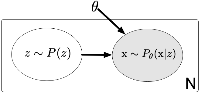
Figure 1: Typical latent variable graphical model. Gray nodes represent observed variables while white nodes represent unobserved variables.

Typically, latent variables models are solved through maximum likelihood estimation which can be formalized as:

$$\max_{\bm{\theta}}\ \log P_{\theta}(\bm{\mathrm{x}})=\max_{\bm{\theta}}\ \log\int P_{\bm{\theta}}(\bm{\mathrm{x}}|\bm{z})P(\bm{z})d\bm{z}\ =\max_{\bm{\theta}}\ \log\mathbb{E}_{\bm{z}}[P_{\bm{\theta}}(\bm{\mathrm{x}}|\bm{z})]$$ (1)

In many cases, the expectation from Equation 1 does not have a closed form solution (eg: non-conjugate distributions) and quadrature is not computationally tractable due to large dimensional spaces [63, 101] (eg: images). To overcome these intractabilities we use a Variational Autoencoder (VAE), which we summarize in Section 3.3. The VAE allows us to infer our latent variables and jointly estimate the parameters of our model. However, before describing the VAE, it is important to understand how this generative setting can be perceived in a lifelong learning scenario.

3.2 Lifelong Generative Modeling

Lifelong generative modeling extends the single-distribution estimation task from Section 3.1 to a set of $i=\{1...L\}$ sequentially observed learning tasks. The $i$-th learning task has variates that are realized from the task specific conditional, $P_{i}(\bm{\mathrm{x}})=P(\bm{\mathrm{x}}|\bm{z}_{d}=i)$, where $\bm{z}_{d}$ acts as a categorical indicator variable of the current task. We visualize a simplified form of this in Figure 2 below.

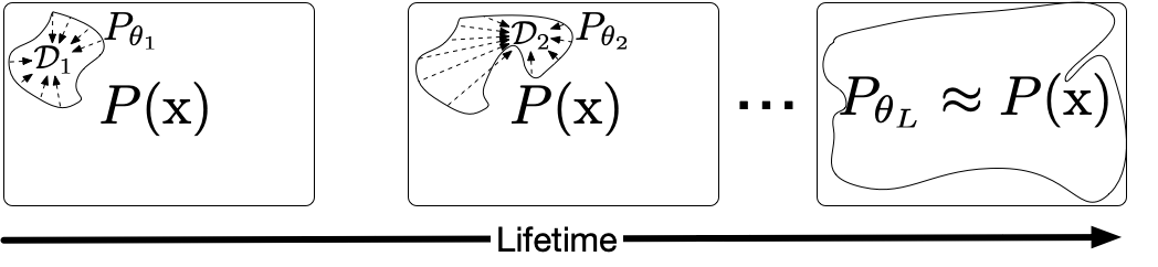
Figure 2: Simplified lifetime of a lifelong learner. Given a true (unknown) distribution, $P(\bm{\mathrm{x}})=\int P(\bm{\mathrm{x}}|\bm{z}_{d})P(\bm{z}_{d})\delta\bm{z}_{d}$, we observe partial information in the form of L sequential tasks, $\{\bm{\mathcal{D}}_{1}\mapsto\bm{\mathcal{D}}_{2},...\mapsto\bm{\mathcal{D}}_{L}\}$. Observing more tasks, reduces the uncertainty of the model until convergence, $P_{\theta_{L}}(\bm{\mathrm{x}})\approx P(\bm{\mathrm{x}})$.

Crucially, when observing task, $\bm{\mathcal{D}}_{i}$, the model has no access to any of the previous task datasets, $\bm{\mathcal{D}}_{<i}$. As the lifelong learner observes more tasks, $\{\bm{\mathcal{D}}_{1}\mapsto\bm{\mathcal{D}}_{2}\mapsto...\mapsto\bm{\mathcal{D}}_{L}\}$, it should improve its estimate of the true distribution, $P_{\theta}(\bm{\mathrm{x}})\approx P(\bm{\mathrm{x}})=\int P(\bm{\mathrm{x}}|\bm{z}_{d})P(\bm{z}_{d})\delta\bm{z}_{d}$, which is unknown at the start of training.

3.3 The Variational Autoencoder

As eluded to in Section 3.1, we would like to infer the latent variables from the data. This can be realized as an alternative form of Equation 1 in the form of Bayes rule: $P_{\bm{\phi}}(\bm{z}|\bm{\mathrm{x}})=P_{\bm{\theta}}(\bm{\mathrm{x}}|\bm{z})P(\bm{z})/P_{\bm{\theta}}(\bm{\mathrm{x}})$, where $P_{\bm{\phi}}(\bm{z}|\bm{\mathrm{x}})$ is referred to as the latent variable posterior and $P_{\bm{\theta}}(\bm{\mathrm{x}}|\bm{z})$ as the likelihood. One method of approximating the posterior, $P_{\bm{\phi}}(\bm{z}|\bm{\mathrm{x}})$, is through MCMC sampling methods such as Gibbs sampling [34] or Hamiltonian MCMC [87]. MCMC methods have the advantage that they provide asymptotic guarantees [88] of convergence to the true posterior, $P_{\phi}(\bm{z}|\bm{\mathrm{x}})$. However in practice it is not possible to know when convergence has been achieved. In addition, due to their Markovian nature, they possess an inner loop, which makes it challenging to scale for large scale datasets.

In contrast, Variational Inference (VI) [55] side-steps the intractability of the posterior by approximating it with a tractable distribution family, $Q_{\bm{\phi}}(\bm{z}|\bm{\mathrm{x}})$. VI rephrases the objective of determining the posterior as an optimization problem by minimizing the KL divergence between the known distributional family, $Q_{\bm{\phi}}(\bm{z}|\bm{\mathrm{x}})$, and the unknown true posterior, $P_{\bm{\theta}}(\bm{z}|\bm{\mathrm{x}})$. Applying VI to the intractable integral from Equation 1 results in the evidence lower bound (ELBO) or variational free energy, which can easily be derived from first principles:

$$\log P_{\bm{\theta}}(\bm{\mathrm{x}}) =\log\int P_{\bm{\theta}}(\bm{\mathrm{x}}|\bm{z})P(\bm{z})d\bm{z}$$ (2)

$$=\log\int\frac{Q_{\bm{\phi}}(\bm{z}|\bm{\mathrm{x}})}{Q_{\bm{\phi}}(\bm{z}|\bm{\mathrm{x}})}P_{\bm{\theta}}(\bm{\mathrm{x}}|\bm{z})P(\bm{z})d\bm{z}$$ (3)

$$\geq\underbrace{\mathbb{E}_{Q}[\log P_{\bm{\theta}}(\bm{\mathrm{x}}|\bm{z})]-\mathbb{D}_{KL}[Q_{\bm{\phi}}(\bm{z}|\bm{\mathrm{x}})||P(\bm{z})]}_{\text{ELBO}}$$ (4)

where we used Jensen’s inequality to transition from Equation 3 to Equation 4. The objective introduced in Equation 4 induces the graphical model shown below in Figure 3.

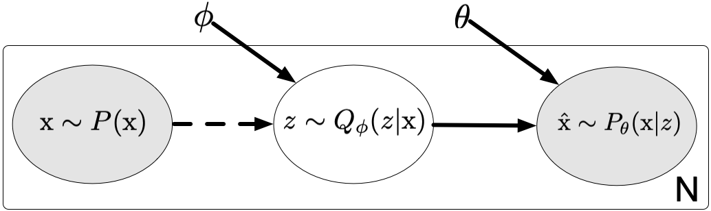
Figure 3: Standard VAE graphical model. Gray nodes represent observed variables while white nodes represent unobserved variables; dashed lines represent inferred variables.

VAEs typically use deep neural networks to model the approximate inference network, $Q_{\bm{\phi}}(\bm{z}|\bm{\mathrm{x}})$ and conditional, $P_{\bm{\theta}}(\bm{\mathrm{x}}|\bm{z})$, which are also known as the encoder and decoder networks (respectively). To optimize for the parameters of these networks, VAEs maximize the ELBO (Equation 4) using Stochastic Gradient Descent [103]. By sharing the variational parameters of the encoder, $\bm{\phi}$, across the data points (amortized inference [35]), variational autoencoders avoid per-data inner loops typically needed by MCMC approaches.

Optimizing the ELBO in Equation 4 requires computing the gradient of an expectation over the approximate posterior, $Q_{\bm{\phi}}(\bm{z}|\bm{\mathrm{x}})$. This typically takes place through the use of the path-wise estimator [101, 63] (originally called “push-out” [106]). The path-wise reparameterizer uses the Law of the Unconscious Statistician (LOTUS) [42], which enables us to compute the expectation of a function of a random variable (without knowing its distribution) if we know its corresponding sampling path and base distribution [84]. For the typical isotropic gaussian approximate posterior, $Q_{\bm{\phi}}(\bm{z}|\bm{\mathrm{x}})$, used in standard VAEs this can be aptly summarized by:

$$\bm{z}\sim Q_{\bm{\phi}}(\bm{z}|\bm{\mathrm{x}}) \Leftrightarrow\bm{\mu}_{\phi}(\bm{\mathrm{x}})+\bm{\sigma}_{\bm{\phi}}(\bm{\mathrm{x}})\epsilon,\ \ \epsilon\sim\mathcal{N}(0,1)$$ (5)

$$\nabla_{\bm{\phi}}\mathbb{E}_{Q_{\bm{\phi}}(\bm{z}|\bm{\mathrm{x}})}[\log P_{\bm{\theta}}(\bm{\mathrm{x}}|\bm{z})] \Leftrightarrow\mathbb{E}_{\underbrace{\mathcal{N}(\epsilon|0,1)}_{\text{base distribution}}}[\nabla_{\bm{\phi}}\log P_{\bm{\theta}}(\bm{\mathrm{x}}|\underbrace{\bm{\mu}_{\phi}(\bm{\mathrm{x}})+\bm{\sigma}_{\bm{\phi}}(\bm{\mathrm{x}})\epsilon}_{\text{sampling path}})]$$ (6)

where Equation 5 defines the sampling procedure of our latent variable through the location-scale transformation and Equation 6 defines the path-wise Monte Carlo gradient estimator applied on the decoder (first term in Equation 4). This Monte Carlo estimator enables differentiating through the sampling process of the distribution $Q_{\bm{\phi}}(\bm{z}|\bm{\mathrm{x}})$. Note that computing the gradient of the second term in Equation 4, $\nabla_{\bm{\phi}}\mathbb{D}_{KL}[Q_{\bm{\phi}}(\bm{z}|\bm{\mathrm{x}})||P(\bm{z})]$, is possible through a closed form analytical solution for the case of isotropic gaussian distributions.

While it is possible to extend any latent variable generative model to the lifelong setting, we choose to build our lifelong generative models using variational autoencoders (VAEs) [63] as they provide a mechanism for stable training; this contrasts other state of the art unsupervised models such as Generative Adversarial Networks (GANs) [39, 61]. Furthermore, latent-variable posterior approximations are a requirement in many learning scenarios such as clustering [93], compression [92] and unsupervised representation learning [30]. Finally, GANs can suffer from low sample diversity [28] which can lead to compounding errors in a lifelong generative setting.

4 Lifelong Learning Model

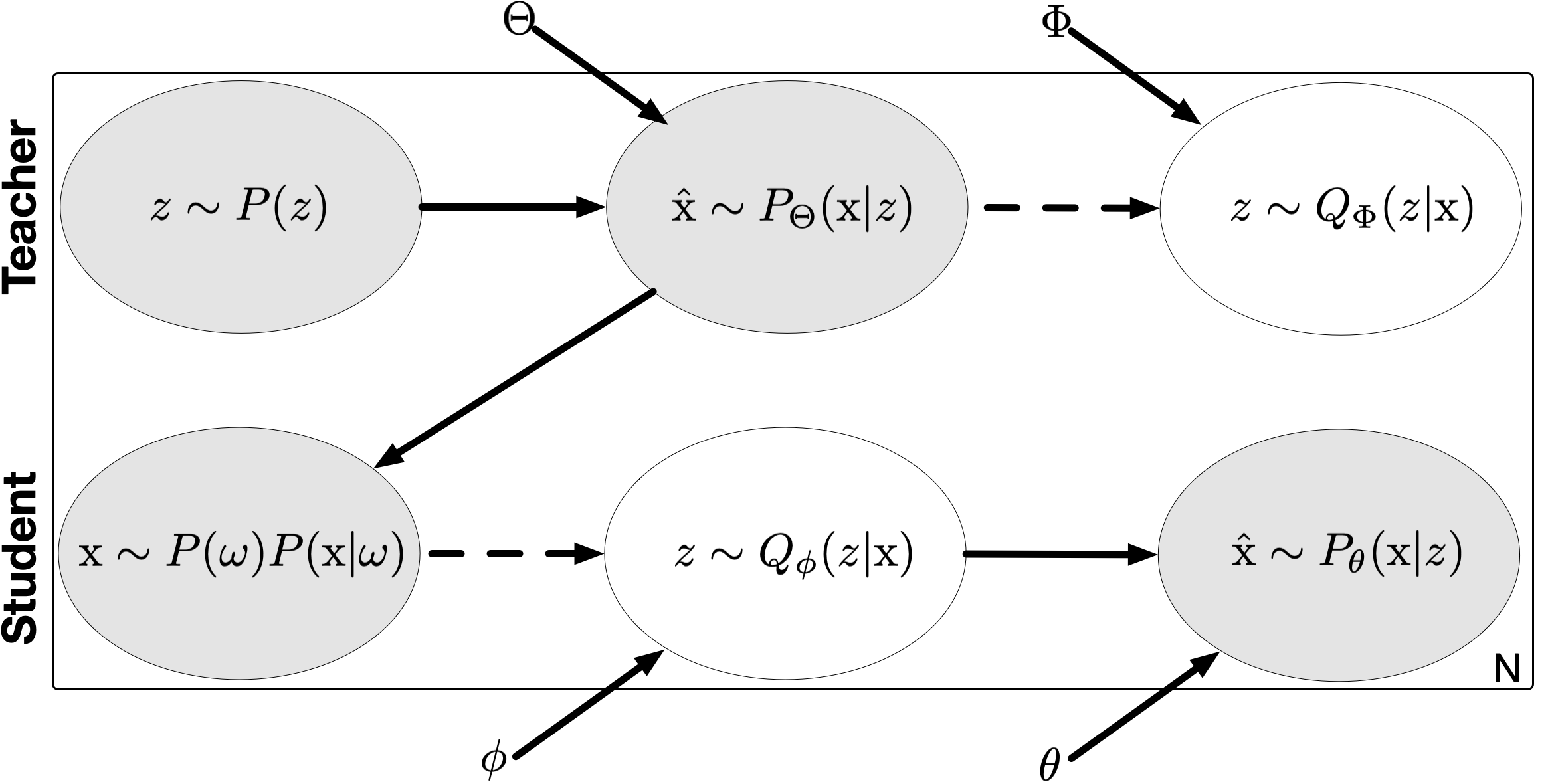
Algorithm 1 Data Flow

  Teacher:

  Sample Prior: $\bm{z}_{j}\sim P(\bm{z})$

  Decode: $\hat{\bm{\mathrm{x}}}_{j}\sim P_{\bm{\Theta}}(\bm{\mathrm{x}}|\bm{z})$

  

  Student:

  Sample : $\bm{\mathrm{x}}_{j}\sim P(\bm{\omega})P(\bm{\mathrm{x}}|\bm{\omega})$

  Encode : $\bm{z}_{j}\sim Q_{\bm{\phi}}(\bm{z}|\bm{\mathrm{x}})$

  Decode: $\hat{\bm{\mathrm{x}}}_{j}\sim P_{\bm{\theta}}(\bm{\mathrm{x}}|\bm{z})$

Figure 4: Student training procedure. Left: graphical model for student-teacher model. Data generated from the teacher model (top row) is used to augment the current training data observed by the student model (bottom row). A posterior regularizer is also applied between $Q_{\bm{\phi}}(\bm{z}|\bm{\mathrm{x}})$ and $Q_{\bm{\Phi}}(\bm{z}|\bm{\mathrm{x}})$ to enable functional regularization (not shown, but discussed in detail in Section 4.1.1). Right: data flow algorithm.

fMRI studies of the rodent [119, 53, 58] and human [110] brains have shown that previously experienced sequences of events are replayed in the hippocampus during rest. These replays are necessary for better planning [53] and memory consolidation [16]. We take inspiration from the memory consolidation of biological learners and introduce our model of Lifelong Generative Modeling (LGM). We visualize the LGM student-teacher architecture in Figure 4.

The student and the teacher are both instantiations of the same base-level generative model, but have different roles throughout the learning process. The teacher’s role is to act as a probabilistic knowledge store of previously learned distributions, which it transfers to the student in the form of replay and functional regularization. The student’s role is to learn the distribution over the new task, while accommodating the learned representation of the teacher over old tasks. In the following sections we provide detailed descriptions of the student-teacher architecture, as well as the base-level generative model that each of them use. The base-level model uses a variant of VAEs, which we tailor for lifelong learning and is learned by maximizing a variant of the standard VAE ELBO from Equation 4 ; we describe this objective at end of this section.

4.1 Student-teacher Architecture

The top row of Figure 4 represents the teacher model. At any given time, the teacher contains a summary of all previous distributions within the learned parameters, $\bm{\Phi}$, of the encoder $Q_{\bm{\Phi}}(\bm{z}|\bm{\mathrm{x}})$, and the learned parameters, $\bm{\Theta}$, of the decoder $P_{\bm{\Theta}}(\bm{\mathrm{x}}|\bm{z})$. We use the teacher to generate synthetic variates, $\hat{\bm{\mathrm{x}}}_{j}$, from these past distributions by decoding variates from the prior, $\bm{z}_{j}\sim P(\bm{z})\mapsto P_{\bm{\Theta}}(\bm{\mathrm{x}}|\bm{z}=\bm{z}_{j})$. We pass the generated (synthetic) variates, $\hat{\bm{\mathrm{x}}}_{j}$, to the student model as a form of knowledge transfer about the past distributions. Information transfer in this manner is known as generative replay and our work is the first to explore it in a VAE setting.

The bottom row of Figure 4 represents the student. The student is responsible for updating the parameters, $\bm{\phi}$, of its encoder, $Q_{\bm{\phi}}(\bm{z}|\bm{\mathrm{x}})$, and $\bm{\theta}$, of its decoder $P_{\bm{\theta}}(\bm{\mathrm{x}}|\bm{z})$. Importantly, the student receives data from both the currently observed task, as well as synthetic data generated by the teacher. This can be formalized as $\bm{\mathrm{x}}_{j}\sim P(\bm{\omega})P(\bm{\mathrm{x}}|\bm{\omega}),\,\bm{\omega}\sim\text{Ber}(\pi)$, as shown in Equation 7:

$$P(\bm{\omega})P(\bm{\mathrm{x}}|\bm{\omega})=\begin{cases}P_{\bm{\Theta}}(\bm{\mathrm{x}}|\bm{z})&\bm{\omega}=0\\ P_{i}(\bm{\mathrm{x}})&\bm{\omega}=1\end{cases}$$ (7)

The mean, $\pi$, of the Bernoulli distribution, controls the sampling proportion of the previously learned distributions to the current one and is set based on the number of assimilated distributions. Thus, given $i$ observed distributions: $\pi=\frac{1}{i+1}$. This ensures that the samples observed by the student are representative of both the current and past distributions. Note that this does not correspond to varying sample sizes in datasets, but merely our assumption to model each distribution with equivalent weighting.

Once a new task is observed, the old teacher is dropped, the student model is frozen and becomes the new teacher ($\bm{\phi}\to\bm{\Phi},\bm{\theta}\to\bm{\Theta}$). A new student is then instantiated with the latest weights $\bm{\phi}$ and $\bm{\theta}$ from the previous student (the new teacher). Due to the cyclic nature of this process, no new models are added. This contrasts many existing state of the art deep lifelong learning methods which add an entire new model or head-network per task (eg: [91, 94, 123]).

A crucial aspect in the lifelong learning process is to ensure that previous learning is successfully exploited to bias current learning [126]. While the replay mechanism that we put in place ensures that the student will observe data from all tasks, it does not ensure that previous knowledge from the teacher is efficiently exploited to improve current student learning. The student model will re-learn (from scratch) a completely new representation, which might be different than the teacher. In order to successfully transfer knowledge between both VAE models, we rely on functional regularization, which we enforce through a Bayesian update regularizer of the posteriors of both models. Intuitively, we would like the student model’s latent outputs, $\bm{z}_{j}\sim Q_{\bm{\phi}}(\bm{z}|\bm{\mathrm{x}})$ to be similar to latent outputs of teacher model, $\bm{z}_{j}\sim Q_{\bm{\Phi}}(\bm{z}|\bm{\mathrm{x}})$, over synthetic variates generated by the teacher, $\bm{\mathrm{x}}_{j}\sim P(\bm{\omega})P(\bm{\mathrm{x}}|\bm{\omega}=0)=P_{\bm{\Theta}}(\bm{\mathrm{x}}|\bm{z})$. In the following section, we describe the exact functional form of this regularizer and demonstrate how it can be perceived as a natural extension of the VAE learning objective to a sequential setting.

4.1.1 Knowledge Transfer Via Bayesian Update.

While both the student and teacher are instantiations of VAE variants, tailored for the particularities of the lifelong setting, for the purpose of this exposition we use the standard VAE formulation. Our objective is to learn the set of parameters $[\bm{\phi},\bm{\theta}]$ of the student, such that it can generate variates from the complete distribution, $P(\bm{\mathrm{x}})$, described in Section 3.2. Subsuming the definition of the augmented input data, $\bm{\mathrm{x}}\sim P(\bm{\omega})P(\bm{\mathrm{x}}|\bm{\omega})$, from Equation 7, we can define the student ELBO as:

$${\mathcal{L}}_{\bm{\theta},\bm{\phi}}(\bm{\mathrm{x}})= \ \mathbb{E}_{Q_{\bm{\phi}}(\bm{z}|\bm{\mathrm{x}})}\bigg{[}\log P_{\bm{\theta}}(\bm{\mathrm{x}}|\bm{z})\bigg{]}-\text{KL}[Q_{\bm{\phi}}(\bm{z}|\bm{\mathrm{x}})||P(\bm{z})],$$ (8)

$$\bm{\mathrm{x}}\sim P(\bm{\omega})P(\bm{\mathrm{x}}|\bm{\omega}),\,\bm{\omega}\sim\text{Ber}(\pi).$$

Rather than naively shrinking the full posterior to the prior via the KL divergence in Equation 8, we rely on one of the core tenets of the Bayesian paradigm which states that we can always update our posterior when given new information (“yesterday’s posterior is today’s prior”) [79]. Given this tenet, we introduce our posterior regularizer :

$$KL[Q_{\bm{\phi}}(\bm{z}|{\bm{\mathrm{x}}})||Q_{\bm{\Phi}}(\bm{z}|{\bm{\mathrm{x}}})],\ \bm{\mathrm{x}}\sim P(\bm{\mathrm{x}}|\bm{\omega=0})$$ (9)

which distills the teacher’s learnt representation into the student over the generated data only. Combining Equations 8 and 9, yields the objective that we can use to train the student and is described below in Equation 10:

$${\mathcal{L}}_{\bm{\theta},\bm{\phi}}(\bm{\mathrm{x}})= \ \mathbb{E}_{Q_{\bm{\phi}}(\bm{z}|\bm{\mathrm{x}})}\bigg{[}\log P_{\bm{\theta}}(\bm{\mathrm{x}}|\bm{z})\bigg{]}-\text{KL}[Q_{\bm{\phi}}(\bm{z}|\bm{\mathrm{x}})||P(\bm{z})]$$ (10)

$$+(1-\omega)\text{KL}[Q_{\bm{\phi}}(\bm{z}|{\bm{\mathrm{x}}})||Q_{\bm{\Phi}}(\bm{z}|{\bm{\mathrm{x}}})],$$

$$\bm{\mathrm{x}}\sim P(\bm{\omega})P(\bm{\mathrm{x}}|\bm{\omega}),\,\bm{\omega}\sim\text{Ber}(\pi)$$

Note that this is not the final objective, due to the fact that we have yet to present the VAE variant tailored to the particularities of the lifelong setting. We will now show how the posterior regularizer can be perceived as a natural extension of the VAE learning objective, through the lens of a Bayesian update of the student posterior.

Lemma 1

For random variables $\bm{\mathrm{x}}$ and $\bm{z}$ with conditionals $Q_{\bm{\Phi}}(\bm{z}|\bm{\mathrm{x}})$ and $Q_{\bm{\phi}}(\bm{z}|\bm{\mathrm{x}})$, both distributed as a categorical or gaussian and parameterized by $\bm{\Phi}$ and $\bm{\phi}$ respectively, the KL divergence between the distributions is:

$$\begin{split}KL[Q_{\bm{\phi}}(\bm{z}|\bm{\mathrm{x}})||Q_{\bm{\Phi}}(\bm{z}|\bm{\mathrm{x}})]=KL[Q_{\hat{\bm{\phi}}}(\bm{z}|\bm{\mathrm{x}})||P(\bm{z})]+C(\bm{\Phi})\end{split}$$ (11)

where $\hat{\bm{\phi}}=f(\bm{\phi},\bm{\Phi})$ depends on the parametric form of Q, and C is only a function of the parameters, $\bm{\Phi}$.

We prove Lemma 1 for the relevant distributions (under some mild assumptions) in Appendix 10.1. Using Lemma 1 allows us to rewrite Equation 10 as shown below in Equation 12:

$${\mathcal{L}}_{\bm{\theta},\bm{\phi}}(\bm{\mathrm{x}})= \ \mathbb{E}_{Q_{\bm{\phi}}(\bm{z}|\bm{\mathrm{x}})}\bigg{[}\log P_{\bm{\theta}}(\bm{\mathrm{x}}|\bm{z})\bigg{]}-\text{KL}[Q_{\bm{\phi}}(\bm{z}|\bm{\mathrm{x}})||P(\bm{z})]$$ (12)

$$+(1-\omega)\bigg{[}\text{KL}[Q_{\hat{\bm{\phi}}}(\bm{z}|{\bm{\mathrm{x}}})||P(\bm{z})]+C(\bm{\Phi})\bigg{]},$$

$$\bm{\mathrm{x}}\sim P(\bm{\omega})P(\bm{\mathrm{x}}|\bm{\omega}),\,\bm{\omega}\sim\text{Ber}(\pi)$$

This rewrite makes it easy to see that our posterior regularizer from Equation 10 is a standard VAE ELBO (Equation 4) under a reparameterization of the student parameters, $\hat{\bm{\phi}}=f(\bm{\phi},\bm{\Phi})$. Note that $C(\bm{\Phi})$ is constant with respect to the student parameters, $\bm{\phi}$, and thus not used during optimization. While the change seems minor, it omits the introduction of $f(\bm{\phi},\bm{\Phi})$ which allows for a transfer of information between models. In practice, we simply analytically evaluate $KL[Q_{\bm{\phi}}(\bm{z}|\bm{\mathrm{x}})\ ||Q_{\bm{\Phi}}(\bm{z}|\bm{\mathrm{x}})]$, the KL divergence between the teacher and the student posteriors, instead of deriving the functional form of $f(\bm{\phi},\bm{\Phi})$ for each different distribution pair. We present Equation 12 simply as a means to provide a more intuitive understanding of our functional regularizer.

4.2 Base-level generative model.

While it is theoretically possible to use the vanilla VAE from Section 3.3 for the teacher and student models, doing so brings to light a number of limitations that render it problematic for use in the context of lifelong learning (visualized in Figure 5-Right). Specifically, using a standard VAE decoder, $P_{\bm{\theta}}(\bm{\mathrm{x}}|\bm{z})$, to generate synthetic replay data for the student is problematic due to two reasons:

1. Mixed Distributions: Sampling the continuous standard normal prior, $\mathcal{N}(0,1)$, can select a point in latent space that is in between two separate distributions, causing generation of unrealistic synthetic data and eventually leading to loss of previously learnt distributions.

2. Undersampling: Data points mapped to the isotropic-gaussian posterior that are further away from the prior mean will be sampled less frequently, resulting in an undersampling of some of the constituent distributions.

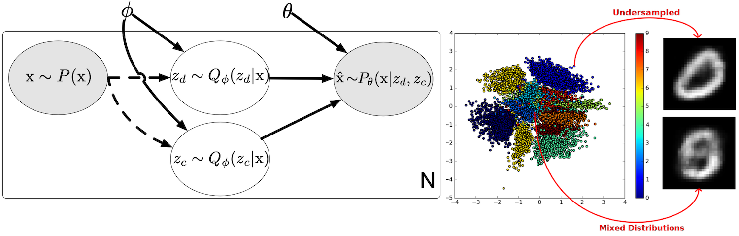
Figure 5: Left: Graphical model for VAE with independent discrete and continuous posterior, $Q_{\bm{\phi}}(\bm{z}_{c},\bm{z}_{d}|\bm{\mathrm{x}})=Q_{\bm{\phi}}(\bm{z}_{c}|\bm{\mathrm{x}})Q_{\bm{\phi}}(\bm{z}_{d}|\bm{\mathrm{x}})$. Right: Two dimensional test variates, $\bm{z}_{j}\sim Q_{\bm{\phi}}(\bm{z}|\bm{\mathrm{x}})$, $\bm{z}_{j}\in\mathbb{R}^{2}$, of a vanilla VAE trained on MNIST. We depict the two generative shortcomings visually: 1) mixing of distributions which causes aliasing in a lifelong setting and 2) undersampling of distributions in a standard isotropic-gaussian VAE posterior.

To address these sampling limitations we decompose the latent variable, $\bm{z}$, into an independent continuous, $\bm{z}_{c}\sim Q_{\bm{\phi}}(\bm{z}_{c}|\bm{\mathrm{x}})$, and a discrete component, $\bm{z}_{d}\sim Q_{\bm{\phi}}(\bm{z}_{d}|\bm{\mathrm{x}})$, as shown in Equation 13 and visually in Figure 5-Left:

$$Q_{\bm{\phi}}(\bm{z}_{c},\bm{z}_{d}|\bm{\mathrm{x}})=Q_{\bm{\phi}}(\bm{z}_{c}|\bm{\mathrm{x}})Q_{\bm{\phi}}(\bm{z}_{d}|\bm{\mathrm{x}}).$$ (13)

The objective of the discrete component is to summarize the discriminative information of the individual generative distributions. The continuous component on the other hand, caters for the remaining sample variability (a nuisance variable [73]). Given that the discrete component can accurately summarize the discriminative information, we can then explicitly sample from any of the past distributions, allowing us to balance the student model’s synthetic inputs with samples from all of the previous learned distributions. We describe this beneficial generative sampling property in more detail in Section 4.2.1.

Naively introducing the discrete component, $\bm{z}_{d}$, does not guarantee that the decoder will use it to represent the most discriminative aspects of the modeled distribution. In preliminary experiments, we observed that that the decoder typically learns to ignore the discrete component and simply relies on the continuous variable, $\bm{z}_{c}$. This is similar to the posterior collapse phenomenon which has received a lot of recent interest within the VAE community [99, 40]. Posterior collapse occurs when training a VAE with a powerful decoder model such as a PixelCNN++ [127] or RNN [21, 40]. The output of the decoder, $\bm{\mathrm{x}}_{j}\sim P_{\bm{\theta}}(\bm{\mathrm{x}}|\bm{z})$ can become almost independent of the posterior sample, $\bm{z}_{j}\sim Q_{\bm{\phi}}(\bm{z}|\bm{\mathrm{x}})$, but is still able to reconstruct the original sample by relying on its auto-regressive property [40]. In Section 4.2.2, we introduce a mutual information regulariser which ensures that the discrete component of the latent variable is not ignored.

4.2.1 Controlled Generations.

Desired Task Conditional $\bm{z}_{c}$ $\bm{z}_{d}$ $P_{1}(\bm{\mathrm{x}})=P(\bm{\mathrm{x}}|\bm{z}_{d}=1)$ $\sim\mathcal{N}(0,1)$ [0, 0, 1] $P_{2}(\bm{\mathrm{x}})=P(\bm{\mathrm{x}}|\bm{z}_{d}=2)$ $\sim\mathcal{N}(0,1)$ [0, 1, 0] $P_{3}(\bm{\mathrm{x}})=P(\bm{\mathrm{x}}|\bm{z}_{d}=3)$ $\sim\mathcal{N}(0,1)$ [1, 0, 0]

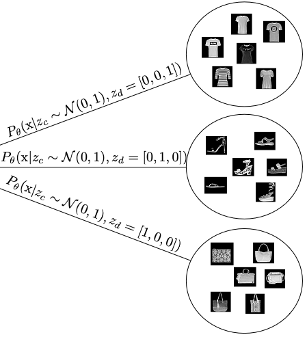
[table]A table beside a figure

Figure 6: FashionMNIST with $L=3$ tasks: t-shirts, sandals and bag. To generate samples from the $i$-th task conditional, $P_{i}(\bm{\mathrm{x}})=P(\bm{\mathrm{x}}|\bm{z}_{d}=i)$, we set $\bm{z}_{d}=i$, randomly sample $\bm{z}_{c}\sim\mathcal{N}(0,1)$, and run $[\bm{z}_{c},\bm{z}_{d}]$ through the decoder, $P_{\bm{\theta}}(\bm{\mathrm{x}}|\bm{z}_{c},\bm{z}_{d})$. Resampling $\bm{z}_{c}$, while keeping $\bm{z}_{d}$ fixed, enables generation of varied samples from the task conditional. Left: Desired task conditionals. Right: Desired decoder behavior.

Given the importance of generative replay for knowledge transfer in LGM, synthetic sample generation by the teacher model needs to be representative of all the previously observed distributions in order to prevent catastrophic forgetting. Under the assumption that $\bm{z}_{d}$ accurately captures the underlying discriminativeness of the individual distributions and through the definition of the LGM generative process, shown in Equation 14:

$$P_{\bm{\Theta}}(\bm{\mathrm{x}}|\bm{z}_{d},\bm{z}_{c}),\ \bm{z}_{c}\sim\mathcal{N}(0,1),\ \bm{z}_{d}\sim Cat(1/L),$$ (14)

we can control generations by setting a fixed value, $\bm{z}_{d}=i$, and randomly sampling the continuous prior, $\bm{z}_{c}\sim\mathcal{N}(0,1)$. This is possible because the trained decoder approximates the task conditional from Section 3.2:

$$P(\bm{\mathrm{x}}|\bm{z}_{d}=i)=P_{i}(\bm{\mathrm{x}}) \approx\frac{P_{\bm{\Theta}}(\bm{\mathrm{x}}|\bm{z}_{c},\bm{z}_{d}=i)P(\bm{z}_{c})}{Q_{\bm{\Phi}}(\bm{z}_{c}|\bm{\mathrm{x}})}$$ (15)

where sampling the true task conditional, $P_{i}(\bm{\mathrm{x}})$, can be approximated by sampling $\bm{z}_{c}\sim P(\bm{z}_{c})=\mathcal{N}(0,1)$, keeping $\bm{z}_{d}$ fixed, and decoding the variates as shown in Equation 16 below:

$$\hat{\bm{\mathrm{x}}}\sim P_{\bm{\Theta}}(\bm{\mathrm{x}}|\bm{z}_{c}\sim\mathcal{N}(0,1),\bm{z}_{d}=i).$$ (16)

We provide a simple example of our desired behavior for three generative tasks, $L=3$, using Fashion MNIST in Figure 6 and Table 2 above. The assumption made up till now is that $\bm{z}_{d}$ accurately captures the discriminative aspects of each distribution. However, there is no theoretical reason for the model to impose this constraint on the latent variables. In practice, we often observe that the decoder $P_{\bm{\theta}}(\bm{\mathrm{x}}|\bm{z}_{c},\bm{z}_{d})$ ignores $\bm{z}_{d}$ due to the much richer representation of the continuous variable, $\bm{z}_{c}$. In the following section we introduce a mutual information constraint that encourages the model to fully utilize $\bm{z}_{d}$.

4.2.2 Information restricting regularizer

As eluded to in the previous section, the synthetic samples observed by the student model need to be representative of all previous distributions. In order to control sampling via the process described in Section 4.2.1, we need to enforce that the discrete variable, $\bm{z}_{d}$, carries the discriminative information about each distribution. Given our graphical model from Figure 4-Left, we observe that there are two ways to accomplish this: maximize the information content between the discrete random variable, $\bm{z}_{d}$ and the decoded $\hat{\bm{\mathrm{x}}}$, or minimize the information content between the continuous variable, $\bm{z}_{c}$ and the decoded $\hat{\bm{\mathrm{x}}}$. Since our graphical model and underlying network does not contain skip connections, information from the input, $\bm{\mathrm{x}}$, has to flow through the latent variables $\bm{z}=[\bm{z}_{c},\bm{z}_{d}]$ to reach the decoder. While both formulations can theoretically achieve the same objective, we observed that in practice, minimizing $I(\hat{\bm{\mathrm{x}}},\bm{z}_{c})$ provided better results. We believe the reason for this is that minimizing $I(\hat{\bm{\mathrm{x}}},\bm{z}_{c})$ provides the model with more subtle gradient information in contrast to maximizing $I(\hat{\bm{\mathrm{x}}},\bm{z}_{d})$ which receives no gradient information when the value of the $k$-th element of the categorical sample is 1. We now formalize our mutual information regularizer, which we derive from first principles in Equation 17:

$\displaystyle\mathbb{E}_{\bm{\mathrm{x}}\sim P_{i}(\bm{\mathrm{x}})}[I(\hat{\bm{\mathrm{x}}},\bm{z}_{c})]$ $\displaystyle=\mathbb{E}_{\bm{\mathrm{x}}\sim P_{i}(\bm{\mathrm{x}})}[H(\bm{z}_{c})-H(\bm{z}_{c}|\hat{\bm{\mathrm{x}}})]$ (17) $\displaystyle=\underbrace{\mathbb{E}_{\bm{\mathrm{x}}\sim P_{i}(\bm{\mathrm{x}})}\mathbb{E}_{\bm{z}_{c}\sim Q_{\bm{\phi}}(\bm{z}_{c}|\bm{\mathrm{x}})}\bigg{[}-\log Q_{\bm{\phi}}(\bm{z}_{c}|\bm{\mathrm{x}})\bigg{]}}_{\mathbb{E}_{\bm{\mathrm{x}}\sim P_{i}(\bm{\mathrm{x}})}[H(\bm{z}_{c})]}$ $\displaystyle\hskip 93.95122pt+$ $\displaystyle\hskip 14.45377pt\underbrace{\mathbb{E}_{\bm{\mathrm{x}}\sim P_{i}(\bm{\mathrm{x}})}\mathbb{E}_{(\bm{z}_{d},\bm{z}_{c})\sim Q_{\bm{\phi}}(\bm{z}_{c},\bm{z}_{d}|\bm{\mathrm{x}})}\bigg{[}\mathbb{E}_{\hat{\bm{\mathrm{x}}}\sim P_{\bm{\theta}}(\hat{\bm{\mathrm{x}}}|\bm{z}_{c},\bm{z}_{d})}\log Q_{\bm{\phi}}(\bm{z}_{c}|\hat{\bm{\mathrm{x}}})\bigg{]}}_{\mathbb{E}_{\bm{\mathrm{x}}\sim P_{i}(\bm{\mathrm{x}})}[-H(\bm{z}_{c}|\hat{\bm{\mathrm{x}}})]},$

where we use the independence assumption of our posterior from Equation 13 and the fact that the expectation of a constant is the constant. This regularizer has parallels to the regularizer in InfoGAN [18]. In contrast to InfoGAN, VAEs already estimate the posterior $Q_{\bm{\phi}}(\bm{z}_{c}|\bm{\mathrm{x}})$ and thus do not need the introduction of any extra parameters $\bm{\phi}$ for the approximation. In addition [47] demonstrated that InfoGAN uses the variational bound (twice) on the mutual information, making its interpretation unclear from a theoretical point of view. In contrast, our regularizer has a clear interpretation: it restricts information through a specific latent variable within the computational graph. We observe that this constraint is essential for empirical performance of our model and empirically validate this in our ablation study in Experiment 7.2.

4.3 Learning Objective

The final learning objective for each of the student models is the maximization of the sequential VAE ELBO (Equation 10), coupled with generative replay (Equation 7)and the mutual information regularizer, $I(\hat{\bm{\mathrm{x}}},\bm{z}_{c})$, (Equation 17):

$$\mathcal{L}_{\bm{\theta},\bm{\phi}}(\bm{\mathrm{x}}) =\ \underbrace{\mathbb{E}_{Q_{\bm{\phi}}(\bm{z}_{c},\bm{z}_{d}|\bm{\mathrm{x}})}\bigg{[}\log P_{\bm{\theta}}(\bm{\mathrm{x}}|\bm{z}_{c},\bm{z}_{d})\bigg{]}-\text{KL}[Q_{\bm{\phi}}(\bm{z}_{c},\bm{z}_{d}|\bm{\mathrm{x}})||P(\bm{z}_{c},\bm{z}_{d})]}_{\text{VAE ELBO}}$$ (18)

$$\hskip 52.63759pt+\underbrace{(1-\omega)\text{KL}[Q_{\bm{\phi}}(\bm{z}_{c},\bm{z}_{d}|{\bm{\mathrm{x}}})||Q_{\bm{\Phi}}(\bm{z}_{c},\bm{z}_{d}|{\bm{\mathrm{x}}})]}_{\text{Posterior Consistency Regularizer}}$$

$$\hskip 101.00728pt-\underbrace{\lambda I(\hat{\bm{\mathrm{x}}},\bm{z}_{c})}_{\text{Mutual Information}},$$

$$\hskip 85.35826pt\bm{\mathrm{x}}\sim P(\bm{\omega})P(\bm{\mathrm{x}}|\bm{\omega}),\,\bm{\omega}\sim\text{Ber}(\pi)$$

The $\lambda$ hyper-parameter controls the importance of the information gain regularizer. Too large a value for $\lambda$ causes a lack of sample diversity, while too small a value causes the model to not use the discrete latent distribution. We did a random hyperparameter search and determined $\lambda=0.01$ to be a reasonable choice for all of our experiments. This is in line with the $\lambda$ used in InfoGAN [18] for continuous latent variables. We empirically validate the necessity of both terms proposed in Equation 18 in our ablation study in Experiment 7.2. We also validate the benefit of the latent variable factorization in Experiment 7.1. Before delving into the experiments, we provide a theoretical analysis of computational complexity induced by our model and objective (Equation 18) in Section 4.4 below.

4.4 Computational Complexity

We define the computational complexity of a typical VAE encoder and decoder as $O(E)$ and $O(D)$ correspondingly; internally these are dominated by the matrix-vector products which take approximately $LO(n^{2})$ for L layers. We also define the cost of applying the loss function as $O(K)+O(R)$, where $O(K)$ is the cost of evaluating the KL divergence from the ELBO (Equation 4) and $O(R)$ the cost for evaluating the reconstruction term. Given these definitions, we can summarize LGM’s computation complexity as follows in Equation 19:

$\displaystyle\underbrace{O(D)}_{\begin{subarray}{c}\text{teacher}\\ \text{generations}\end{subarray}}+\underbrace{O(E)+O(D)}_{\begin{subarray}{c}\text{student encode}\\ \text{+ decode}\end{subarray}}+\underbrace{O(K)+O(R)}_{\text{vae loss}}+\underbrace{O(K)}_{\begin{subarray}{c}\text{posterior}\\ \text{regularizer}\end{subarray}}+\underbrace{O(K)+O(E)}_{\text{mutual info}}$ $\displaystyle=2[O(D)+O(E)]+3[O(K)]+O(R),$ (19)

where we introduce increased computational complexity due to teacher generations, the cost of the posterior regularizer, and the mutual information terms; the latter of which necessitates an extra encode operation, $O(E)$. The computational complexity is still dominated by the matrix-vector product from evaluating forward functionals of the neural network. These operations can easily be amortized through parallelization on modern GPUs and typical experiments do not directly scale as per Equation 19. In our most demanding experiment (Experiment 6.6), we observe an average empirical increase of 13.53 seconds per training epoch and 6.3 seconds per test epoch.

5 Revisiting state of the art methods.

In this section we revisit some of the state of the art methods from Section 2. We begin by providing a mathematical description of the differences between EWC [65], VCL [91] and LGM and follow it up with a discussion of VASE [1] and their extensions of our work.

EWC and VCL: Our posterior regularizer, $KL[Q_{\bm{\phi}}(\bm{z}|{\bm{\mathrm{x}}})||Q_{\bm{\Phi}}(\bm{z}|{\bm{\mathrm{x}}})]$, affects the same parameters, $\bm{\phi}$, as parameter regularizer methods such as EWC and VCL. However, rather than assuming a functional form for the parameter posterior, $P(\bm{\phi}|\bm{\mathrm{x}})$, our method regularizes the output latent distribution $Q_{\bm{\phi}}(\bm{z}|\bm{\mathrm{x}})$. EWC and VCL, both make the assumption that $P(\bm{\phi}|\bm{\mathrm{x}})$ is distributed as an isotropic gaussian. This allows the use of the Fisher Information Matrix (FIM) in a quadratic parameter regularizer in EWC, and an analytical KL divergence of the posterior in VCL. This is a very stringent requirement for the parameters of a neural network and there is active research in Bayesian neural networks that attempts to relax this constraint [74, 75, 80].

EWC $\ \ \ \min_{\bm{\phi}}d[P(\bm{\phi}|\bm{\mathrm{x}})||P(\bm{\Phi}|\bm{\mathrm{x}})]$	LGM ( Isotropic Gaussian Posterior ) $\ \ \ \min_{\bm{\phi}}d[Q_{\bm{\phi}}(\bm{z}|\bm{\mathrm{x}})||Q_{\bm{\Phi}}(\bm{z}|\bm{\mathrm{x}})]$
$\approx\frac{\gamma}{2}(\bm{\phi}-\bm{\Phi})^{T}F(\bm{\phi}-\bm{\Phi})$	$=0.5\bigg{[}tr(\bm{\Sigma_{\bm{\Phi}}}^{-1}\bm{\Sigma_{\bm{\phi}}})+(\bm{\mu_{\bm{\Phi}}}-\bm{\mu_{\bm{\phi}}})^{T}\bm{\Sigma_{\bm{\Phi}}}^{-1}(\bm{\mu_{\bm{\Phi}}}-\bm{\mu_{\bm{\phi}}})-C+log\bigg{(}\frac{|\bm{\Sigma_{\bm{\Phi}}}|}{|\bm{\Sigma_{\bm{\phi}}}|}\bigg{)}\bigg{]}$

In the above table we examine the distance metric $d$, used to minimize the effects of catastrophic inference in both EWC and LGM. While our method can operate over any distribution that has a tractable KL-divergence, for the purposes of demonstration we examine the simple case of an isotropic gaussian latent-variable posterior. EWC directly enforces a quadratic constraint on the model parameters $\bm{\phi}$, while our method indirectly affects the same parameters through a regularization of the posterior distribution $Q_{\bm{\phi}}(\bm{z}|\bm{\mathrm{x}})$. For any given input variate, $\bm{\mathrm{x}}_{j}$, LGM allows to model to freely change its internal parameters, $\bm{\phi}$; it does so in a non-linear way such that the analytical KL shown above is minimized.

VASE : The recent work of Life-Long Disentangled Representation Learning with Cross-Domain Latent Homologies (VASE) [1] extend upon our work [1, p. 7], but take a more empirical route by incorporating a classification-based heuristic for their posterior distribution. In contrast, we show (Section 4.1.1) that our objective naturally emerges in a sequential learning setting for VAEs, allowing us to infer the discrete posterior, $Q_{\bm{\phi}}(\bm{z}_{d}|\bm{\mathrm{x}})$ in an unsupervised manner. Due to the incorporation of direct supervised class information [1] also observe that regularizing the decoding distribution $P_{\bm{\theta}}(\bm{\mathrm{x}}|\bm{z})$ aids in the learning process, something that we observe to fail in a purely unsupervised generative setting (Appendix Section 10.2). Finally, in contrast to [1], we include an information restricting regularizer (Section 4.2.2) which allows us to directly control the interpretation and flow of information of the learnt latent variables.

6 Experiments

We evaluate our model and the baselines over standard datasets used in other state of the art lifelong / continual learning literature [91, 136, 112, 57, 65, 94]. While these datasets are simple in a traditional classification setting, transitioning to a lifelong-generative setting scales the problem complexity substantially. We evaluate LGM on a set of progressively more complicated tasks (Section 6.2) and provide comparisons against baselines [91, 136, 65, 29, 63] using a set of standard metrics (Section 6.1). All network architectures and other optimization details for our LGM model are provided in Appendix Section 10.3 as well our open-source git repository [98].

6.1 Performance Metrics

To validate the benefit of LGM in a lifelong setting we explore three main performance dimensions: the ability for the model to reconstruct and generate samples from all previous tasks and the ability to learn a common representation over time, thus reducing learning sample complexity. We use three main quantitative performance metrics for our experiments: the log-likelihood importance sample estimate [15, 91], the negative test ELBO, and the Frechet distance metric [44]. In addition, we also provide two auxiliary metrics to validate the benefits of LGM in a lifelong setting: training sample complexity and wall clock time per training and test epoch.

To fairly compare models with varying latent variable configurations, one solution is to marginalize out the latents, $\bm{z}$, during model evaluation / test time: $\int_{\bm{z}}P_{\bm{\theta}}(\bm{\mathrm{x}}|\bm{z})d\bm{z}\approx\sum_{k=1}^{K}P_{\bm{\theta}}(\bm{\mathrm{x}}|\bm{z}=\bm{z}_{k})$. This is realized in practice by using a Monte Carlo approximation (typically K=5000) and is commonly known as the importance sample (IS) log-likelihood estimate [15, 91]. As latent variable and model complexity grows, this estimate tends to become noisier and intractable to compute. For our experiments we use this metric only for the FashionMNIST and MNIST datasets as computing one estimate over 10,000 test samples for a complex model takes approximately 35 hours on a K80 GPU.

In contrast to the IS log-likelihood estimate, the negative test ELBO (Equation 4) is only applicable when comparing models with the same latent variable configurations; it is however much faster to compute. The negative test ELBO provides a lower bound to the test log-likelihood of the true data distribution under the assumed latent variable configuration. One crucial aspect missing from both these metrics is an evaluation of generation quality. We resolve this by using the Frechet distance metric [44] and qualitative image samples.

The Frechet distance metric allows us to quantify the quality and diversity of generated samples by using a pre-trained classifier model to compare the feature statistics (generally under a Gaussianity assumption) between synthetic generated samples and samples drawn from the test set. If the Frechet distance between these two distributions is small, then the generative model is said to be generating realistic images. The Frechet distance between two gaussians (produced by evaluating latent embeddings of a classifier model) with means $\bm{m}_{test},\bm{m}_{gen}$ with corresponding covariances $\bm{C}_{test},\bm{C}_{gen}$ is:

$$||\bm{m}_{test}-\bm{m}_{gen}||_{2}^{2}+Tr(\bm{C}_{test}+\bm{C}_{gen}-2[\bm{C}_{test}\bm{C}_{gen}]^{0.5}).$$ (20)

While the Frechet distance, negative ELBO and IS log-likelihood estimate provide a glimpse into model performance, there exists no conclusive metric that captures the quality of unsupervised generative models [124, 108] and active research suggests a direct trade-off between perceptual quality and model representation [8]. Thus, in addition to the metrics described above, we also provide qualitative metrics in the form of test image reconstructions and image generations. We summarize all used performance metrics in Table 2 below:

Definition Purpoose Lower is better? Negative ELBO Equation 4. Quantitative metric on likelihood / reconstructions. yes Negative Log-Likelihood 5000 (latent) sample Monte Carlo estimate of Equation 4. Quantitative metric on density estimate. yes Frechet Distance Equation 20. Quantitative metric on generations. yes Test Reconstructions $P_{\bm{\theta}}(\bm{\mathrm{x}}|\bm{z}_{c}\sim Q_{\bm{\phi}}(\bm{z}_{c}|\bm{\mathrm{x}}),\bm{z}_{d}\sim Q_{\bm{\phi}}(\bm{z}_{d}|\bm{\mathrm{x}}))$ Qualitative view of reconstructions. N/A Generations $P_{\bm{\theta}}(\bm{\mathrm{x}}|\bm{z}_{d}\sim Cat(1/L),\bm{z}_{c}\sim\mathcal{N}(0,1))$. Qualitative view of generations. N/A #Training Samples # real training samples used for task $i$. Sample Complexity. yes

Table 2: Summary of different performance metrics.

6.2 Data Flow

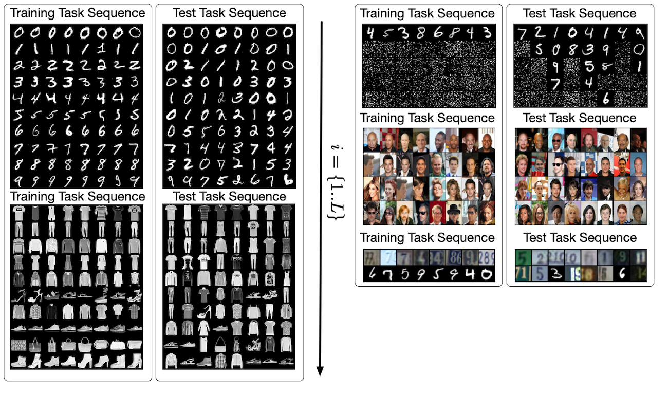
Figure 7: Visual examples of training and test task sequences (top to bottom) for the datasets used to validate LGM. The training set only consists of samples from the current task while the test set is a cumulative union of the current task, coupled with all previous tasks. The permuted MNIST tasks uses $\{G_{1},...G_{L-1}\}$ different fixed permutation matrices to create 4 auxiliary datasets.

In Figure 7 we list train and test variates depicting the data flow for each of the problems that we model. Due to the relaxing the need to preserve data in a lifelong setting, the train task sequence observes a single dataset, $\bm{\mathcal{D}}^{tr}_{i}$, at a time, without access to any previous, $\bm{\mathcal{D}}^{tr}_{<i}$. The corresponding test dataset consists of a union ($\cup$ operator) of the current test dataset, $\bm{\mathcal{D}}^{te}_{i}$, merged with all previously observed test datasets, $\hat{\bm{\mathcal{D}}}^{te}_{i}=\bm{\mathcal{D}}^{te}_{i}\cup\bm{\mathcal{D}}^{te}_{i-1}\cup...\cup\bm{\mathcal{D}}^{te}_{1}$.

MNIST / Fashion MNIST: For the MNIST and Fashion MNIST problems, we observe a single MNIST digit or fashion object (such as shirts) at a time. Each training set consists of 6000 training samples and 1000 test samples. These samples are originally extracted from the full training and test datasets which consist of 60,000 training and 10,000 test samples.

Permuted MNIST: this problem differs from the MNIST problem described above in that we use the entire MNIST dataset at each task. After observing the first task, which is the standard MNIST dataset, each subsequent task differs through the application of a fixed permutation matrix $G_{i}$ on the entire MNIST dataset. The test task sequence differs from the training task sequence in that we simply use the corresponding full train and test MNIST datasets (with the appropriate application of $G_{i}$).

Celeb-A: We split the CelebA dataset into four individual distributions using the features: bald, male, young and eye-glasses. As with the previous problems, we treat each subset of data as an individual distribution, and present our model samples from a single distribution at a time. This presents a real world scenario as the samples per distribution varies drastically from only 3,713 samples for the bald distribution, to 126,788 samples for young. In addition specific samples can span one or more of these distributions.

SVHN to MNIST: in this problem, we transition from fully observing the centered SVHN [89] dataset to observing the MNIST dataset. We treat all samples from SVHN as being generated by one distribution $P_{1}(\bm{\mathrm{x}})$ and all the MNIST samples as generated by another distribution $P_{2}(\bm{\mathrm{x}})$ (irrespective of the specific digit). At inference, the model is required to reconstruct and generate from both datasets.

6.3 Situating against state of the art lifelong learning models.

To situate LGM against other state of the art methods in lifelong learning we use the sequential FashionMNIST and MNIST datasets described earlier in Section 6.2 and the data flow diagram in Figure 7. We contrast our LGM model against VCL [91], VCL without a task specific head network, SI [136], EWC [65], Laplace propagation [29], a full batch VAE trained jointly on all data and a standard naive sequential VAE without any catastrophic forgetting prevention strategy in Figures 8 and 9 below. The full batch VAE presents the upper-bound performance and all lifelong learning models typically under-perform this model by the final learning task. For the baselines, we use the generously open sourced code [90] by the VCL authors, using the optimal hyper-parameters specified for each model. We begin by evaluating the 5000 sample Monte Carlo estimate of the log-likelihood of all compared models in Figure 8 below:

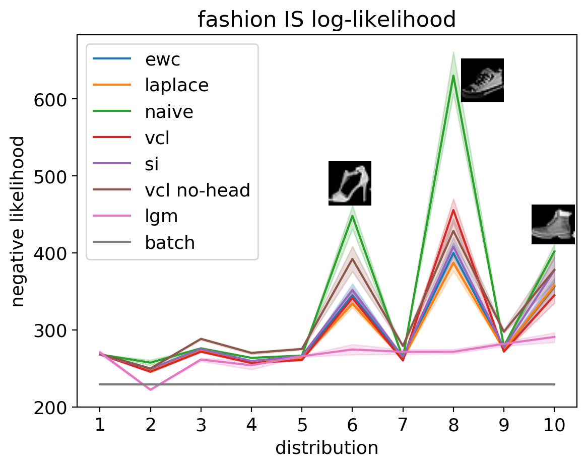
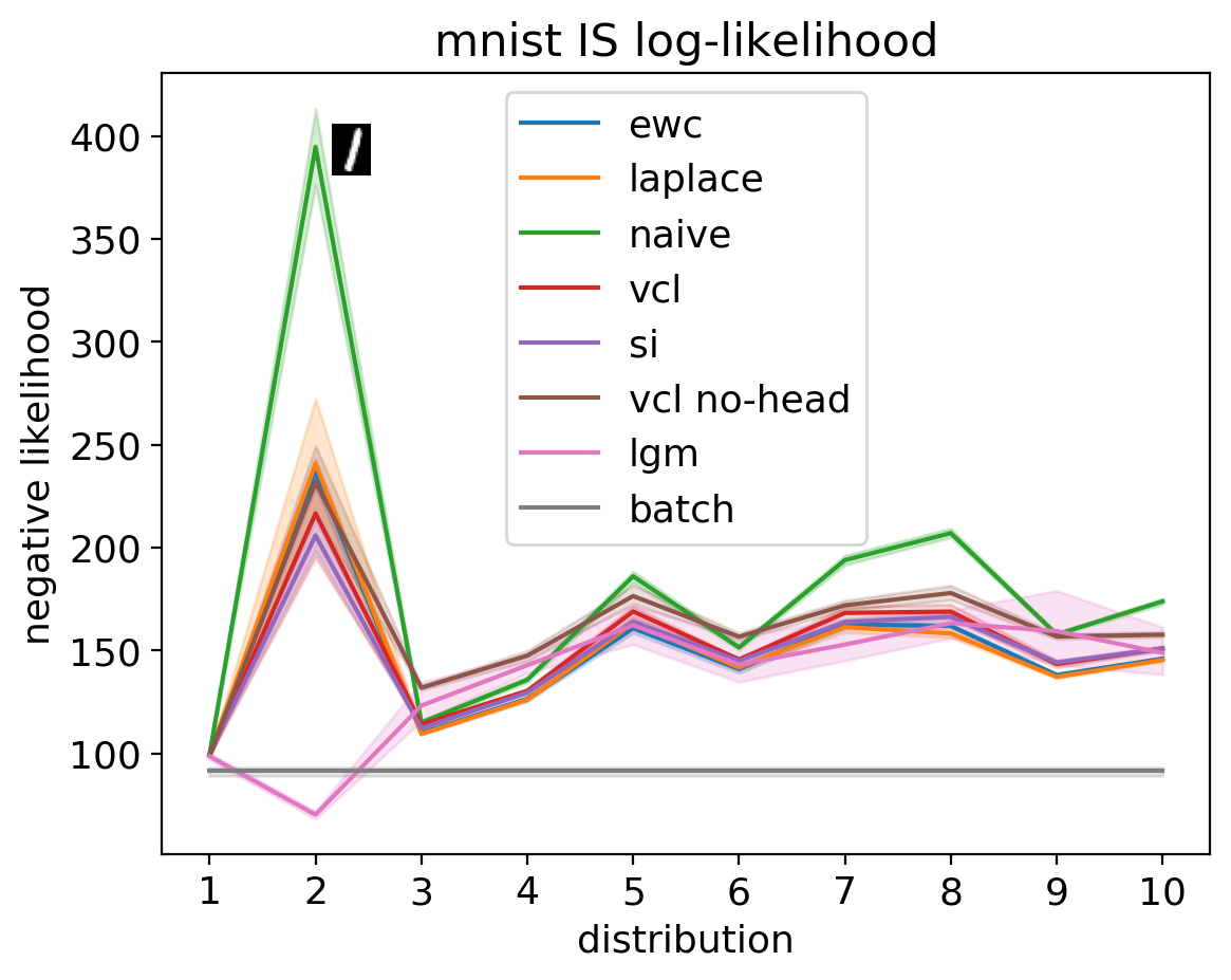
Figure 8: IS log-likelihood (mean $\pm$ std) $\times$ 5. Left: Fashion MNIST. Right: MNIST.

Even though each trial was repeated five times (each), we observe large increases in the estimates at a few critical points. After further inspection, we determined the large magnitude increases were due to the model observing a drastically different distribution at that point. We overlay the graphs with an example variate for of the magnitude spikes. In the case of FashionMNIST for example, the model observes its first shoe distribution at $i=6$; this contrasts the previously observed items which were mainly clothing related objects. Interestingly we observe that LGM has much smoother performance across tasks. We posit this is because LGM does not constrain its parameters, and instead enforces the same input-output mapping through functional regularization.

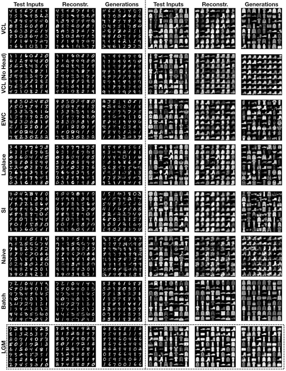
Figure 9: Final model, $i=10$, generation and reconstructions for MNIST and FashionMNIST. The LGM model presents competitive performance for both generations and reconstructions, while not preserving any past data nor past models.

Since one of the core tenets of lifelong learning is to reduce sample complexity over time, we use this experiment to validate if LGM does in fact achieve this objective. Since all LGM models are trained with an early-stopping criterion, we can directly calculate the number of samples used for each learning task using the stopping epoch and mean, $\pi$ of the Bernoulli sampling distribution of the student model. In Figure 10 we plot the number of true samples and the number of synthetic samples used by a model until it satisfied its early-stopping criterion. We observe a steady decrease in the number of real samples used over time, validating LGMs advantage in a lifelong setting.

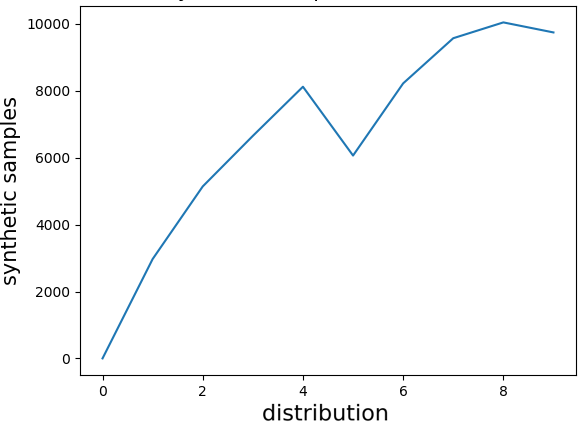
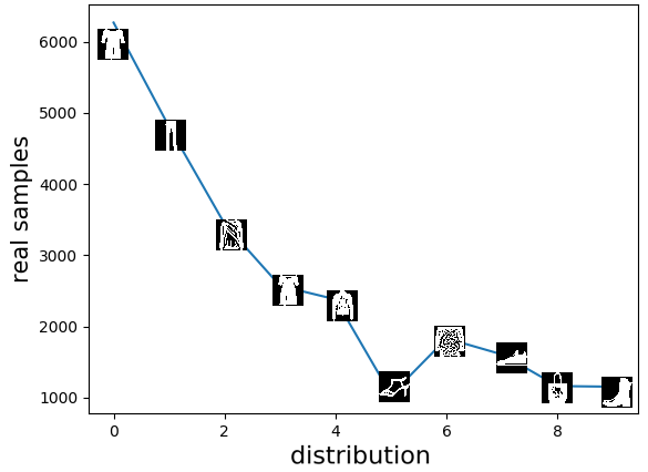
Figure 10: FashionMNIST sample complexity. Left: Synthetic training samples used till early-stopping. Right: Real samples used till early-stopping.

6.4 Diving deeper into the sequence.

Rather than only visualizing the final model’s qualitative results as in Figure 9, we provide qualitative results for model performance over time for the PermutedMNIST experiment in Figure 11. This allows us to visually observe lifelong model performance over time. In this experiment, we focus our efforts on EWC and LGM and visualize model (test) reconstructions starting from the second learning task, $G_{1}\bm{\mathcal{D}}$, till the final $G_{4}\bm{\mathcal{D}}$. The EWC-VAE variant that we use as a baseline has the same latent variable configuration as our model, enabling the usage of the test ELBO as a quantitative metric for comparison. We use an unpermuted version of the MNIST dataset, $\bm{\mathcal{D}}$, as our first distribution, $P_{1}(\bm{\mathrm{x}})$, as it allows us to visually asses the degradation of reconstructions. This is a common setup utilized in continual learning [65, 136] and we extend it here to the density estimation setting.

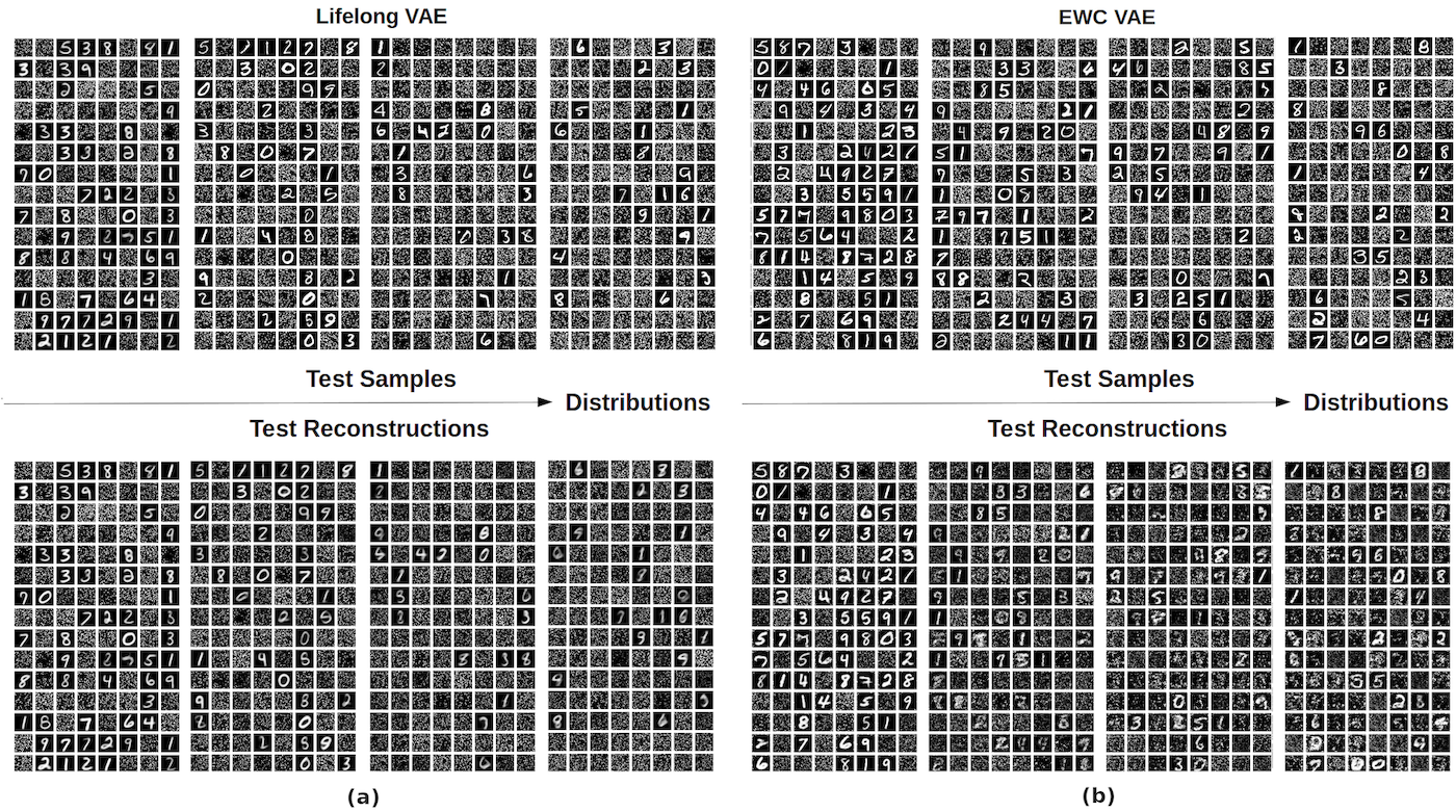
Figure 11: Top row: test-samples; bottom row: reconstructions. We visualize an increasing number of accumulated distributions from left to right. (a) Lifelong VAE model (b) EWC VAE model.

Both models exhibit a different form of degradation: EWC experiences a more destructive form of degradation as exemplified by the salt-and-pepper noise observed in the final dataset reconstruction at $G_{4}\bm{\mathcal{D}}$. LGM on the hand experiences a form of Gaussian noise as visible in the corresponding final dataset reconstruction. In order to numerically quantify this performance we analyze the log-Frechet distance and negative ELBO below in Figure 12, where we contrast the LGM to EWC, a batch VAE (full-vae in graph), an upto-VAE that observes all training data up to the current distribution and a vanilla sequential VAE (vanilla). We examine a variety of different convolutional and dense architectures and present the top performing models below. We observe that LGM drastically outperforms EWC and the baseline naive sequential VAE in both metrics.

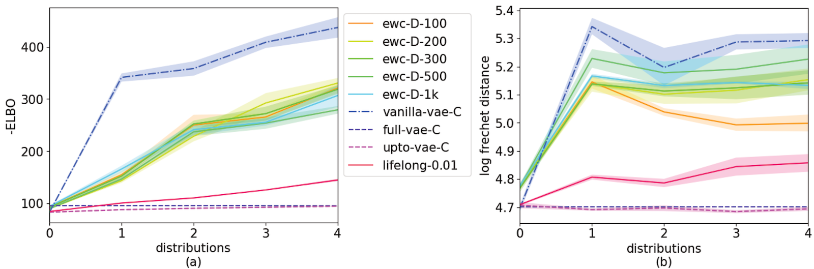
Figure 12: PermutedMNIST (a) negative Test ELBO and (b) log-Frechet distance.

6.5 Learning Across Complex Distributions

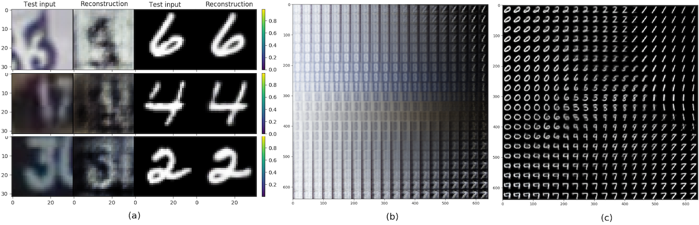
Figure 13: (a) Reconstructions of test samples from SVHN[left] and MNIST[right]; (b) Decoded samples $\hat{\bm{\mathrm{x}}}\sim P_{\bm{\theta}}(\bm{\mathrm{x}}|\bm{z}_{d},\bm{z}_{c})$ based on linear interpolation of $\bm{z}_{c}\in\mathcal{R}^{2}$ with $\bm{z}_{d}=[0,1]$; (c) Same as (b) but with $\bm{z}_{d}=[1,0]$.

The typical assumption in lifelong learning is that the sequence of observed distributions are related [125] in some manner. In this experiment we relax this constraint by learning a common model between the colored SVHN dataset and the binary MNIST dataset. While semantically similar to humans, these datasets are vastly different, as one is based on RGB images of real world house numbers and the other of synthetically hand-drawn digits. We visualize examples of the true test inputs, $\bm{\mathrm{x}}$, and their respective reconstructions, $\hat{\bm{\mathrm{x}}}$, from the final lifelong model in figure 13(a). Even though the only true data the final model received for training was the MNIST dataset, it is still able to reconstruct the SVHN data observed previously. This demonstrates the ability of our architecture to transition between complex distributions while still preserving the knowledge learned from the previously observed distributions.

Finally, in figure 13(b) and 13(c) we illustrate the data generated from an interpolation of a 2-dimensional continuous latent space, $\bm{z}_{c}\in\mathcal{R}^{2}$. To generate variates, we set the discrete categorical, $\bm{z}_{d}$, to one of the possible values $\{[0,1],[1,0]\}$ and linearly interpolate the continuous $\bm{z}_{c}$ over the range $[-3,3]$. We then decode these to obtain the samples, $\hat{\bm{\mathrm{x}}}\sim P_{\bm{\theta}}(\bm{\mathrm{x}}|\bm{z}_{d},\bm{z}_{c})$. The model learns a common continuous structure for the two distributions which can be followed by observing the development in the generated samples from top left to bottom right on both figure 13(b) and 13(c).

6.6 Validating Empirical Sample Complexity Using Celeb-A

We iterate the Celeb-A dataset as described in the data flow diagram (Figure 7) and use this learning task to explore qualitative and quantitative generations, as well as empirical real world time complexity (as described in Section 4.4) on modern GPU hardware. We train a lifelong model and a typical VAE baseline without catastrophic forgetting mitigation strategies and evaluate the final model’s generations in Figure 14. As visually demonstrated in Figure 14-Left, the lifelong model is able to generate instances from all of the previous distributions, however the baseline model catastrophically forgets (Figure 14-Right) and only generates samples from the eye-glasses distribution. This is also reinforced by the log-Frechet distance shown in Figure 15.

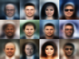
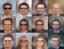
Figure 14: Left: Sequential generations for Celeb-A from the final lifelong model for bald, male, young and eye-glasses (left to right). Right: (random) generations by the final baseline VAE model.

We also evaluate the wall-clock time in seconds (Table 3) for the lifelong model and the baseline-vae for the 44,218 samples of the male distribution. We observe that the lifelong model does not add a significant overhead, especially since the baseline-vae undergoes catastrophic forgetting (Figure 14 Right) and completely fails to generate samples from previous distributions. Note that we present the number of parameters and other detailed model information in our code and Appendix 10.3.

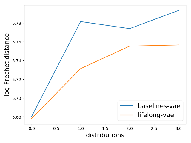
44,218 male samples baseline-VAE Lifelong training-epoch (s) 43.1 +/- 0.6 56.63 +/- 0.28 testing-epoch (s) 9.79 +/- 0.12 16.09 +/- 0.01

Table 3: Mean & standard deviation wall-clock for one epoch of male distribution of Celeb-A.

Figure 15: Celeb-A log-Frechet distance of lifelong vs. naive baseline VAE model without catastrophic mitigation strategies over the four distributions. Listed on the right is the time per epoch (in seconds) for an epoch of the corresponding models.

7 Ablation Studies

In this section we independently validate the benefit of each of the newly introduced components to the learning objective proposed in Section 4.3. In Experiment 7.1 we demonstrate the benefit of the discrete-continuous posterior factorization introduced in Section 4.2.1. Then in Experiment 7.2, we validate the necessity of the information restricting regularizer (Section 4.2.2) and posterior consistency regularizer (Section 4.1.1).

7.1 Linear Separability of Discrete and Continuous Posterior

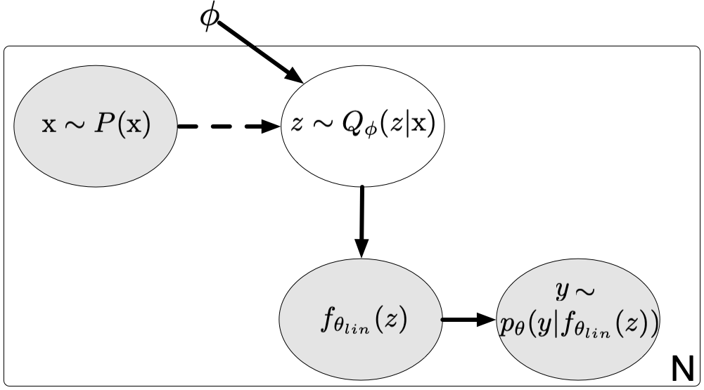
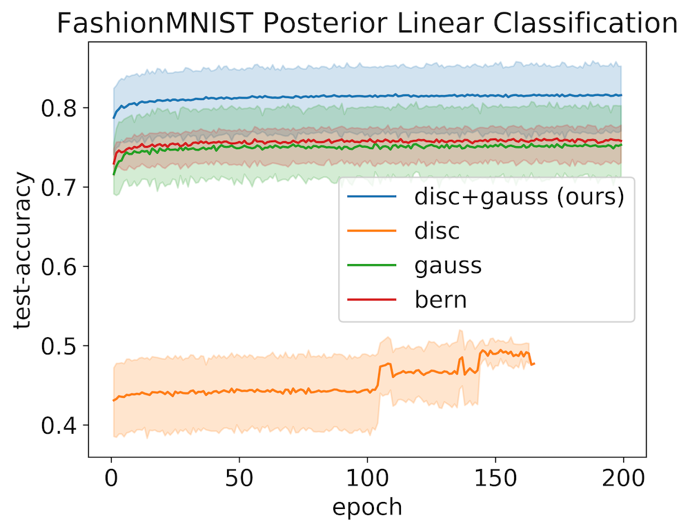
Figure 16: Left: Graphical model depicting classification using pretrained VAE, coupled with a linear classifier, $f_{\bm{\theta}_{lin}}:\bm{z}\mapsto\bm{y}$. Right: Linear classifier accuracy on the Fashion MNIST test set for a varying range of latent dimensions, $|\bm{z}|\in[32,64,128,256,512,1024]$ and distributions.

In order to validate that the (independent) discrete and continuous latent variable posterior, $Q_{\bm{\phi}}(\bm{z}_{d},\bm{z}_{c}|\bm{\mathrm{x}})$, aids in learning a better representation, we classify the encoded posterior sample using a simple linear classifier $f_{\bm{\theta}_{lin}}:\bm{z}\mapsto\bm{y}$, where $\bm{y}$ corresponds to the categorical class prediction. Higher (linear) classification accuracies demonstrate that the the VAE is able to learn a more linearly separable representation. Since the latent representation of VAEs are typically used in auxiliary tasks, learning such a representation is useful in downstream tasks. This is a standard method to measure posterior separability and is used in methods such as Associative Compression Networks [41].

We use the standard training set of FashionMNIST [135] (60,000 samples) to train a standard VAE with a discrete only (disc) posterior, an isotropic-gaussian only (gauss) posterior, a bernoulli only (bern) posterior and finally the proposed independent discrete and continuous (disc+gauss) posterior presented in Section 4.2.1. For each different posterior reparameterization, we train a set of VAEs with varying latent dimensions, $|\bm{z}|\in[32,64,128,256,512,1024]$. In the case of the disc+gauss model we fix the discrete dimension, $|\bm{z}_{d}|=10$ and vary the isotropic-gaussian dimension to match the total required dimension. After training each VAE, we proceed to use the same training data to train a linear classifier on the encoded posterior sample, $\bm{z}\sim Q_{\bm{\phi}}(\bm{z}|\bm{\mathrm{x}})$.

In Figure 16 we present the mean and standard deviation linear test classification accuracies of each set of the different experiments. As expected, the discrete only (disc) posterior performs poorly due to the strong restriction of mapping an entire input sample to a single one-hot vector. The isotropic-gaussian (gauss) and bernoulli (bern) only models provide a strong baseline, but the combination of isotropic-gaussian and discrete posteriors (disc+gauss) performs much better, reaching an upper-bound (linear) test-classification accuracy of 87.1%. This validates that the decoupling of latent represention presented in Section 4.2.1 aids in learning a more meaningful, separable posterior.

7.2 Validating the Mutual Information and Posterior Consistency Regularizers.

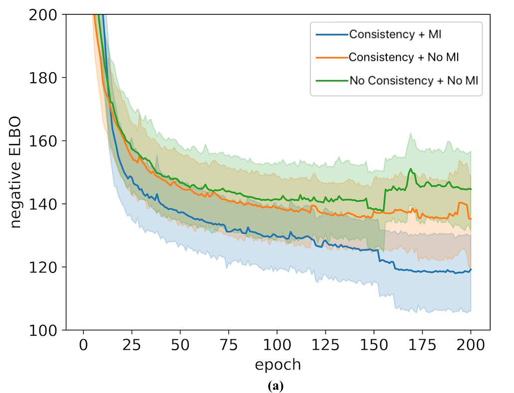
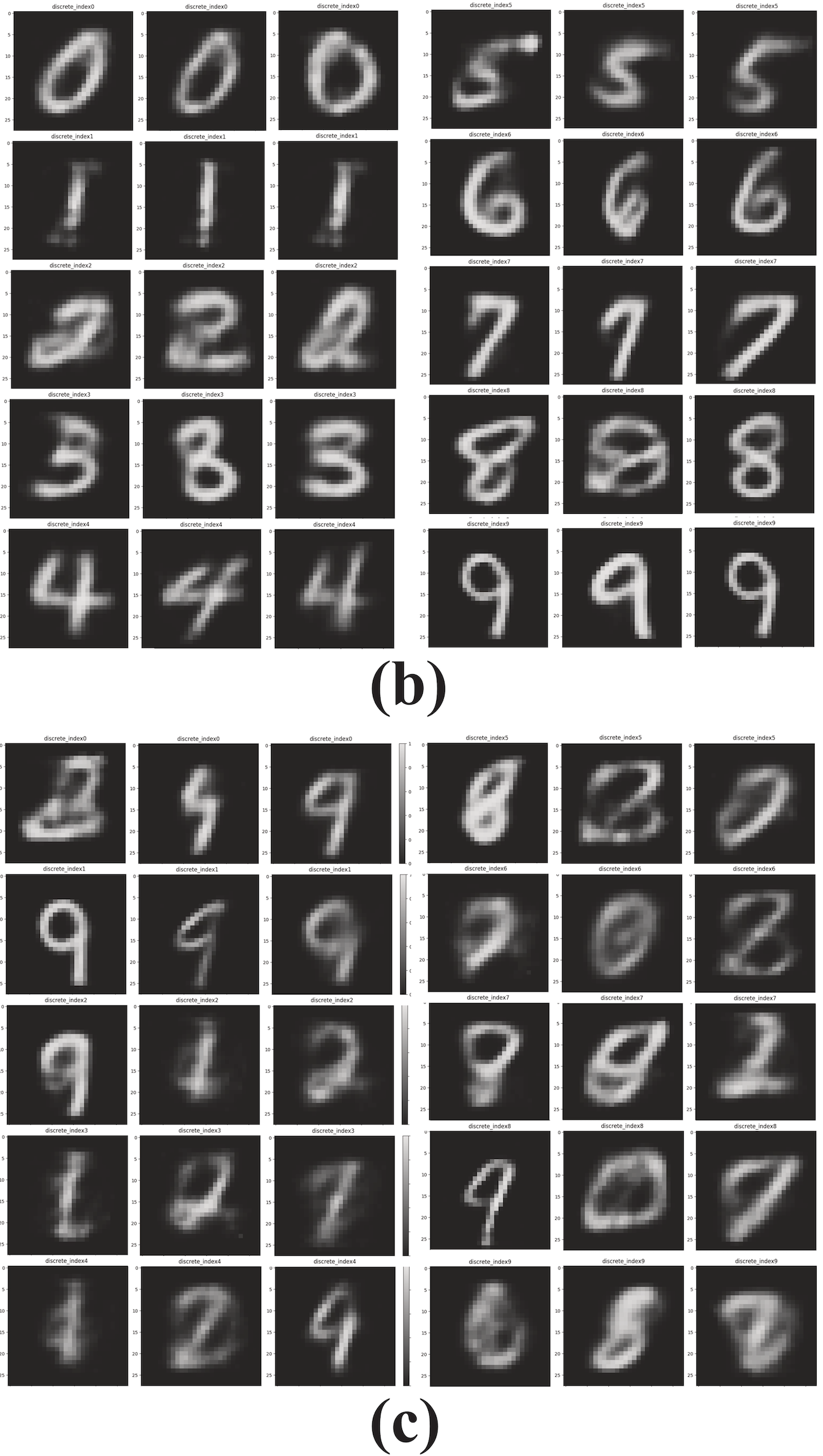
Figure 17: MNIST Ablation: (a) negative test ELBO. (b) Sequentially generated samples by setting $\bm{z}_{d}$ and sampling $\bm{z}_{c}\sim\mathcal{N}(0,1)$ (Section 4.2.1) with consistency + mutual information (MI). (c) Sequentially generated samples with no consistency + no mutual information (MI).

In order to independently evaluate the benefit of our proposed Bayesian update regularizer (Section 4.1.1) and the mutual information regularizer proposed in (Section 4.2.1) we perform an ablation study using the MNIST data flow sequence from Figure 7. We evaluate three scenarios: 1) with posterior consistency and mutual information regularizers, 2) only posterior consistency and 3) without both regularizers. We observe that both components are necessary in order to generate high quality samples as evidenced by the negative test ELBO in Figure 17-(a) and the corresponding generations in Figure 17-(b-c). The generations produced without the information gain regularizer and consistency in Figure 17-(c) are blurry. We attribute this to: 1) uniformly sampling the discrete component is not guaranteed to generate samples representative samples from $P_{<i}(\bm{\mathrm{x}})$ and 2) the decoder, $P_{\bm{\Theta}}(\bm{\mathrm{x}}|\bm{z}_{d},\bm{z}_{c})$, relays more information through the continuous component, $P_{\bm{\Theta}}(\bm{\mathrm{x}}|\bm{z}_{d},\bm{z}_{c})=P_{\bm{\Theta}}(\bm{\mathrm{x}}|\bm{z}_{c})$, causing catastrophic forgetting and posterior collapse [4].

8 Limitations

While LGM presents strong performance, it fails to completely solve the problem of lifelong generative modeling and we see a slow degradation in model performance over time. We attribute this mainly to the problem of poor VAE generations that compound upon each other (also discussed below). In addition, there are a few poignant issues that need to be resolved in order to achieve an optimal (in terms of non-degrading Frechet distance / -ELBO) unsupervised generative lifelong learner:

Distribution Boundary Evaluation: The standard assumption in current lifelong / continual learning approaches [91, 136, 112, 57, 65, 94] is to use known, fixed distributions instead of learning the distribution transition boundaries. For the purposes of this work, we focus on the accumulation of distributions (in an unsupervised way), rather than introduce an additional level of indirection through the incorporation of anomaly detection methods that aid in detecting distributional boundaries.

Blurry VAE Generations: VAEs are known to generate images that are blurry in contrast to GAN based methods. This has been attributed to the fact that VAEs don’t learn the true posterior and make a simplistic assumption regarding the reconstruction distribution $P_{\bm{\theta}}(\bm{\mathrm{x}}|\bm{z})$ [4, 97]. While there exist methods such as ALI [27] and BiGAN [26], that learn a posterior distribution within the GAN framework, recent work has shown that adversarial methods fail to accurately match posterior-prior distribution ratios in large dimensions [104].

Memory: In order to scale to a truly lifelong setting, we posit that a learning algorithm needs a global pool of memory that can be decoupled from the learning algorithm itself. This decoupling would also allow for a principled mechanism for parameter transfer between sequentially learnt models as well a centralized location for compressing non-essential historical data. Recent work such as the Kanerva Machine [133] and its extensions [134] provide a principled way to do this in the VAE setting.

9 Conclusion

In this work we propose a novel method for learning generative models over a lifelong setting. The principal assumption for the data is that they are generated by multiple distributions and presented to the learner in a sequential manner. A key limitation for the learning process is that the method has no access to any of the old data and that it shall distill all the necessary information into a single final model. The proposed method is based on a dual student-teacher architecture where the teacher’s role is to preserve the past knowledge and aid the student in future learning. We argue for and augment the standard VAE’s ELBO objective by terms helping the teacher-student knowledge transfer. We demonstrate the benefits this augmented objective brings to the lifelong learning setting using a series of experiments. The architecture, combined with the proposed regularizers, aid in mitigating the effects of catastrophic interference by supporting the retention of previously learned knowledge.

10 Appendix

10.1 Understanding the Consistency Regularizer

The analytical derivations of the consistency regularizer show that the regularizer can be interpreted as an a transformation of the standard VAE regularizer. In the case of an isotropic gaussian posterior, the proposed regularizer scales the mean and variance of the student posterior by the variance of the teacher 1 and adds an extra ’volume’ term. This interpretation of the consistency regularizer shows that the proposed regularizer preserves the same learning objective as that of the standard VAE. Below we present the analytical form of the consistency regularizer with categorical and isotropic gaussian posteriors:

Proof 1

We assume the learnt posterior of the teacher is parameterized by a centered, isotropic gaussian with $\bm{\Phi}=[\bm{\mu^{E}=\bm{0}},\bm{\Sigma^{E}}=\text{diag}(\bm{\sigma^{E^{2}}})]$ and the posterior of our student by a non-centered isotropic gaussian with $\bm{\phi}=[\bm{\mu^{S}},\bm{\Sigma^{S}}=\text{diag}(\bm{\sigma^{S2}})]$, then

$\displaystyle\begin{split}KL(Q_{\bm{\phi}}(\bm{z}|\bm{x})||Q_{\bm{\Phi}}(\bm{z}|\bm{x}))&=0.5\bigg{[}tr(\bm{\Sigma}^{E^{-1}}\bm{\Sigma^{S}})+(\bm{\mu^{E}}-\bm{\mu^{S}})^{T}\bm{\Sigma}^{E^{-1}}(\bm{\mu^{E}}-\bm{\mu^{S}})-F+log\bigg{(}\frac{|\bm{\Sigma^{E}}|}{|\bm{\Sigma^{S}}|}\bigg{)}\bigg{]}\\ &=0.5\sum_{j=1}^{F}\bigg{[}\frac{1}{\sigma^{E2}(j)}(\sigma^{S2}(j)+\mu^{S2}(j))-1+log\ \sigma^{E2}(j)-log\ \sigma^{S2}(j)\bigg{]}\\ &=KL(Q_{\bm{\phi^{*}}}(\bm{z}|\bm{x})||\mathcal{N}(0,\bm{I}))-log\ |\bm{\Sigma}^{E}|\end{split}$ (21) Via a reparameterization of the student’s parameters: $\displaystyle\begin{split}\bm{\phi}^{*}&=[\bm{\mu}^{S*},\bm{\sigma}^{{S*2}}]\\ \bm{\mu}^{S*}=\frac{\mu^{S}(j)}{\sigma^{E2}(j)}&;\bm{\sigma}^{S*2}=\frac{\sigma^{S2}(j)}{\sigma^{E2}(j)}\end{split}$ (22)

It is also interesting to note that our posterior regularizer becomes the prior if:

$$lim_{\bm{\sigma}^{E^{2}}\mapsto 1}KL(Q_{\bm{\phi}}(\bm{z}|\bm{x})||Q_{\bm{\Phi}}(\bm{z}|\bm{x}))=KL(Q_{\bm{\phi}}(\bm{z}|\bm{x})||\mathcal{N}(0,\bm{I}))$$

Proof 2

We parameterize the learnt posterior of the teacher by $\Phi_{i}=\frac{\exp({p_{i}^{E}})}{\sum_{i=1}^{J}\exp({p_{i}^{E}})}$ and the posterior of the student by $\phi_{i}=\frac{\exp({p_{i}^{S}})}{\sum_{i=1}^{J}\exp({p_{i}^{S}})}$. We also redefine the normalizing constants as $c^{E}=\sum_{i=1}^{J}\exp({p_{i}^{E}})$ and $c^{S}=\sum_{i=1}^{J}\exp({p_{i}^{S}})$ for the teacher and student models respectively. The KL divergence from the ELBO can now be re-written as:

$$\begin{split}KL(Q_{\bm{\phi}}(\bm{z}_{d}|\bm{x})||Q_{\bm{\Phi}}(\bm{z}_{d}|\bm{x}))&={\sum_{i=1}^{J}}\frac{\exp({p_{i}^{S}})}{c^{S}}log\ \bigg{(}\frac{\exp({p_{i}^{S}})}{c^{S}}\frac{c^{E}}{\exp({p_{i}^{E}})}\bigg{)}\\ &=H(\bm{p}^{S},\bm{p}^{S}-\bm{p}^{E})=-H(\bm{p}^{s})+H(\bm{p}^{S},\bm{p}^{E})\end{split}$$ (23)

where $H(\_)$ is the entropy operator and $H(\_,\_)$ is the cross-entropy operator.

10.2 Reconstruction Regularizer

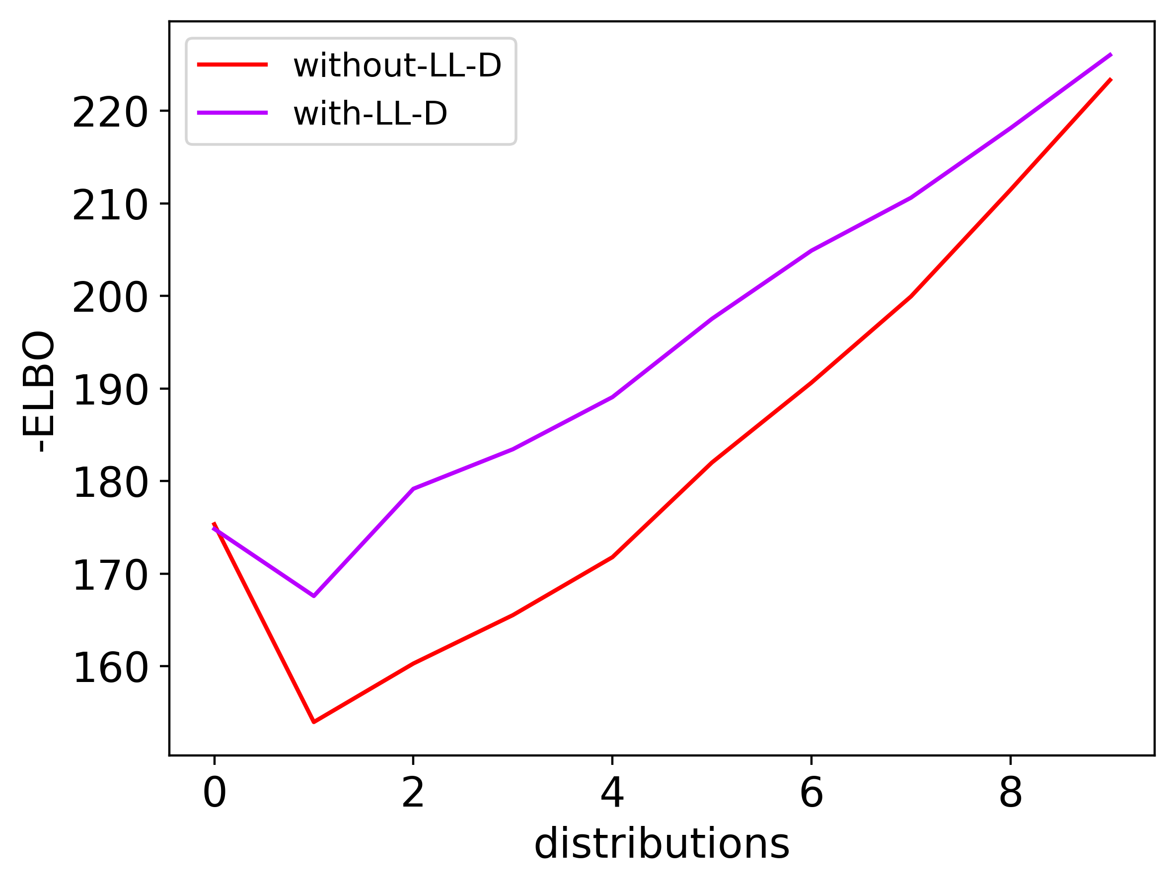
Figure 18: Fashion Negative Test ELBO

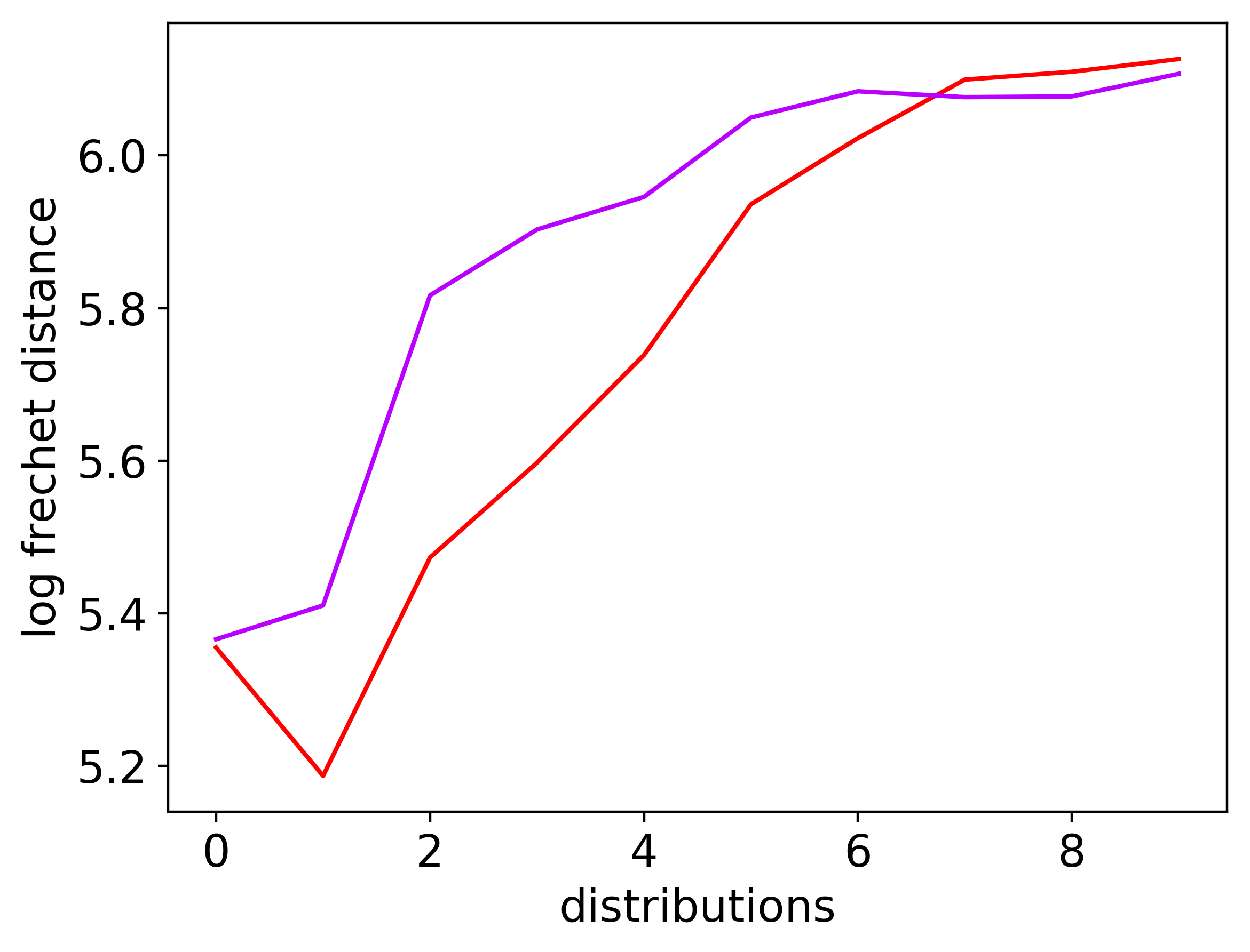
Figure 19: Fashion Log-Frechet Distance

While it is possible to constrain the reconstruction/decoder term of the VAE in a similar manner to the consistency posterior-regularizer, i.e: $KL[P_{\bm{\theta}}(\hat{\bm{\mathrm{x}}}|\bm{z})||P_{\bm{\Theta}}(\hat{\bm{\mathrm{x}}}|\bm{z})]$, doing so diminishes model performance. We hypothesize that this is due to the fact that this regularizer contradicts the objective of the reconstruction term $P_{\bm{\theta}}(\bm{\mathrm{x}}|\bm{z})$ in the ELBO which already aims to minimize some metric between the input samples $\bm{\mathrm{x}}$ and the reconstructed samples $\hat{\bm{\mathrm{x}}}$; eg: if $P_{\bm{\theta}}(\bm{\mathrm{x}}|\bm{z})\sim\mathcal{N}(\bm{\mu},\text{diag}[\bm{\sigma}])$, then the loss is proportional to $||\hat{\bm{\mathrm{x}}}-\bm{\mathrm{x}}||_{2}^{2}$, the standard L2 loss. Without the addition of this reconstruction cross-model regularizer, the model is also provided with more flexibility in how it reconstructs the output samples.

In order to quantify the this we duplicate the FashionMNIST Experiment listed in the data flow definition in Figure 7. We use a simpler model than the main experiments to validate this hypothesis. We train two dense models (-D): one with just the posterior consistency regularizer (without-LL-D) and one with the consistency and likelihood regularizer (with-LL-D). We observe the model performance drops (with respect to the Frechet distance as well the test ELBO) in the case of the with-LL-D as demonstrated in Figures 19 and 19.

10.3 Model Architecture

We used two different architectures for our experiments. When we use a dense network (-D) we used two layers of 512 units to map to the latent representation and two layers of 512 to map back to the reconstruction for the decoder. We used batch norm [48] and ELU activations for all the layers barring the layer projecting into the latent representation and the output layer. Note that while we used the same architecture for EWC we observed a drastic negative effect when using batch norm and thus dropped it’s usage. The convolution architectures (-C) used the architecture described below for the encoder and the decoder (where the decoder used conv-transpose layers for upsampling). The notation is [OutputChannels, (filterX, filterY), stride]:

$$\begin{split}\text{Encoder: }&[32,(5,5),1]\mapsto\text{GN+ELU}\mapsto[64,(4,4),2]\mapsto\text{GN+ELU}\mapsto[128,(4,4),1]\mapsto\\ &\text{GN+ELU}\mapsto[256,(4,4),2]\mapsto\text{GN+ELU}\mapsto[512,(1,1),1]\mapsto\\ &\text{GN+ELU}\mapsto[512,(1,1),1]\\ \text{Decoder: }&[256,(4,4),1]\mapsto\text{GN+ELU}\mapsto[128,(4,4),2]\mapsto\text{GN+ELU}\mapsto[64,(4,4),1]\\ &\mapsto\text{GN+ELU}\mapsto[32,(4,4),2]\mapsto\text{GN+ELU}\mapsto[32,(5,5),1]\\ &\mapsto\text{GN+ELU}\mapsto[\text{chans},(1,1),1]\end{split}$$ (24)

Method	Initial $\bm{z}_{d}$ dimension	Final $\bm{z}_{d}$ dimension	$\bm{z}_{c}$ dimension	# initial parameters	# final parameters
EWC-D	10	10	14	4,353,184	4,353,184
naive-D	10	10	14	1,089,830	1,089,830
batch-D	10	10	14	1,089,830	1,089,830
batch-D	10	10	14	2,179,661	2,179,661
lifelong-D	1	10	14	2,165,311	2,179,661
EWC-C	10	10	14	30,767,428	30,767,428
naive-C	10	10	14	7,691,280	7,691,280
batch-C	10	10	14	7,691,280	7,691,280
batch-C	10	10	14	15,382,560	15,382,560
lifelong-C	1	10	14	15,235,072	15,382,560

The table above lists the number of parameters for each model and architecture used in our experiments. The lifelong models initially start with a $\bm{z}_{d}$ of dimension 1 and at each step we grow the representation by one dimension to accommodate the new distribution (more info in Section 10.7). In contrast, the baseline EWC models are provided with the full representation throughout the learning process. EWC has double the number of parameters because the computed diagonal fisher information matrix which is the same dimensionality as the number of parameters. EWC also neeeds the preservation of the teacher model $[\bm{\Phi},\bm{\Theta}]$ to use in it’s quadratic regularizer. Both the naive and batch models have the fewest number of parameters as they do not use a student-teacher framework and only use one model, however the vanilla model has no protection against catastrophic interference and the full model is just used as an upper bound for performance.

We used Adam [62] to optimize all of our problems with a learning rate of 1e-4 or 1e-3. When we used weight transfer we re-initialized the accumulated momentum vector of Adam as well as the aggregated mean and variance of the batch norm layers. The full architecture can be examined in our github repository [98] and is provided under an MIT license.

10.4 Contrast to streaming / online methods

Our method has similarities to streaming methods such as Streaming Variational Bayes (SVB) [14] and Incremental Bayesian Clustering methods [60, 38] in that we estimate and refine posteriors through time. In general this can be done through the following Bayesian update rule that states that the lastest posterior is proportional to the current likelihood times the previous posterior:

$$P(\bm{z}|\bm{\mathrm{X}}_{1},...,\bm{\mathrm{X}}_{t})\propto P(\bm{\mathrm{X}}_{t}|\bm{z})P(\bm{z}|\bm{\mathrm{X}}_{1},...,\bm{\mathrm{X}}_{t-1})$$ (25)

SVB computes the intractable posterior, $P(\bm{z}|\bm{\mathrm{X}}_{1},...,\bm{\mathrm{X}}_{t})$, utilizing an approximation, $\mathcal{A}_{t}$, that accepts as input the current dataset, $\bm{\mathrm{X}}_{t}$, along with the previous posterior $\mathcal{A}_{t-1}$ :

$$P(\bm{z}|\bm{\mathrm{X}}_{1},...,\bm{\mathrm{X}}_{t})\approx\mathcal{A}_{t}(\bm{\mathrm{X}}_{t},\mathcal{A}_{t-1})$$ (26)

The first posterior input ($\mathcal{A}_{t=0}$) to the approximating function is the prior $P(\bm{z})$. The objective of SVB and other streaming methods is to model the posterior of the currently observed data in the best possible manner. Our setting differs from this in that we want to retain information from all previously observed distributions (sometimes called a knowledge store [126]). This can be useful in scenarios where a distribution is seen once, but only used much later down the road. Rather than creating a posterior update rule, we recompute the posterior via Equation 25, leveraging the fact that we can re-generate $\bm{\mathrm{X}}_{<t}\approx\bm{\hat{\mathrm{X}}}_{<t}$ through the generative process. This allows us to recompute a more appropriate posterior re-using all of the (generated) data, rather than using the previously computed (approximate) posterior $\mathcal{A}_{t-1}$:

$$P(\bm{z}|\bm{\mathrm{X}}_{1},\bm{\mathrm{X}}_{2},...,\bm{\mathrm{X}}_{t})\propto P(\bm{\mathrm{X}}_{t}|\bm{z})P(\bm{z}|\bm{\hat{\mathrm{X}}}_{1},...,\bm{\hat{\mathrm{X}}}_{t-1})$$ (27)

Coupling this generative replay strategy with the Bayesian update regularizer introduced in Section 4.1.1, we demonstrate that not only do we learn an updated poster as in Equation 27, but also allow for a natural transfer of information between sequentially learnt models: a fundamental tenant of lifelong learning [126, 125].

Finally, another key difference between lifelong learning and online methods is that lifelong learning aims to learn from a sequence of tentatively different [20] tasks while still retaining and accumulating knowledge; online learning generally assumes that the true underlying distribution comes from a single distribution [11]. There are some exceptions to this where online learning is applied to the problem of domain adaptation, eg: [49, 60].

10.5 EWC Baselines: Comparing Conv & Dense Networks

We compared a whole range of EWC baselines and use the best performing models few in our experiments. Listed in Figure 10.5 are the full range of EWC baselines run on the PermutedMNIST and FashionMNIST experiments. Recall that C / D describes whether a model is convolutional or dense and the the number following is the hyperparameter for the EWC or Lifelong VAE.

10.6 Gumbel Reparameterization

Since we model our latent variable as a combination of a discrete and a continuous distribution we also use the Gumbel-Softmax reparameterization [76, 50]. The Gumbel-Softmax reparameterization over logits [linear output of the last layer in the encoder] $\bm{p}\in\mathcal{R}^{M}$ and an annealed temperature parameter $\tau\in\mathcal{R}$ is defined as:

$$\bm{z} =softmax(\frac{{log(\bm{p})+\bm{g}}}{\tau});\bm{g}=-log(-log(\bm{u}\sim Unif(0,1)))$$ (28)

$\bm{u}\in\mathcal{R}^{M},\bm{g}\in\mathcal{R}^{M}$. As the temperature parameter $\tau\mapsto 0$, $\bm{z}$ converges to a categorical.

10.7 Expandable Model Capacity and Representations

Multilayer neural networks with sigmoidal activations have a VC dimension bounded between $O(\rho^{2})$[120] and $O(\rho^{4})$[59] where $\rho$ are the number of parameters. A model that is able to consistently add new information should also be able to expand its VC dimension by adding new parameters over time. Our formulation imposes no restrictions on the model architecture: i.e. new layers can be added freely to the new student model.

In addition we also allow the dimensionality of $\bm{z}_{d}\in\mathcal{R}^{J}$, our discrete latent representation to grow in order to accommodate new distributions. This is possible because the KL divergence between two categorical distributions of different sizes can be evaluated by simply zero padding the teacher’s smaller discrete distribution. Since we also transfer weights between the teacher and the student model, we need to handle the case of expanding latent representations appropriately. In the event that we add a new distribution we copy all the weights besides the ones immediately surrounding the projection into and out of the latent distribution. These surrounding weights are reinitialized to their standard Glorot initializations [37].

References

- [1] A. Achille, T. Eccles, L. Matthey, C. Burgess, N. Watters, A. Lerchner, and I. Higgins. Life-long disentangled representation learning with cross-domain latent homologies. In Advances in Neural Information Processing Systems, pages 9895–9905, 2018.
- [2] W.-K. Ahn and W. F. Brewer. Psychological studies of explanation—based learning. In Investigating explanation-based learning, pages 295–316. Springer, 1993.
- [3] W.-K. Ahn, R. J. Mooney, W. F. Brewer, and G. F. DeJong. Schema acquisition from one example: Psychological evidence for explanation-based learning. Technical report, Coordinated Science Laboratory, University of Illinois at Urbana-Champaign, 1987.
- [4] A. Alemi, B. Poole, I. Fischer, J. Dillon, R. A. Saurous, and K. Murphy. Fixing a broken elbo. In International Conference on Machine Learning, pages 159–168, 2018.
- [5] J. R. Anderson and G. H. Bower. Human associative memory. Psychology press, 2014.
- [6] D. Bahdanau, K. Cho, and Y. Bengio. Neural machine translation by jointly learning to align and translate. ICLR, 2015.
- [7] H. R. Blackwell. Contrast thresholds of the human eye. JOSA, 36(11):624–643, 1946.
- [8] Y. Blau and T. Michaeli. The perception-distortion tradeoff. In Proceedings of the IEEE Conference on Computer Vision and Pattern Recognition, pages 6228–6237, 2018.
- [9] A. Blum. On-line algorithms in machine learning. In Online algorithms, pages 306–325. Springer, 1998.
- [10] C. Blundell, J. Cornebise, K. Kavukcuoglu, and D. Wierstra. Weight uncertainty in neural network. In International Conference on Machine Learning, pages 1613–1622, 2015.
- [11] L. Bottou. Online learning and stochastic approximations. On-line learning in neural networks, 17(9):142, 1998.
- [12] L. Bottou and Y. L. Cun. Large scale online learning. In Advances in neural information processing systems, pages 217–224, 2004.
- [13] A. Brock, J. Donahue, and K. Simonyan. Large scale GAN training for high fidelity natural image synthesis. In 7th International Conference on Learning Representations, ICLR 2019, New Orleans, LA, USA, May 6-9, 2019, 2019.
- [14] T. Broderick, N. Boyd, A. Wibisono, A. C. Wilson, and M. I. Jordan. Streaming variational bayes. In Advances in Neural Information Processing Systems 26: 27th Annual Conference on Neural Information Processing Systems 2013. Proceedings of a meeting held December 5-8, 2013, Lake Tahoe, Nevada, United States., pages 1727–1735, 2013.
- [15] Y. Burda, R. Grosse, and R. Salakhutdinov. Importance weighted autoencoders. ICLR, 2016.
- [16] M. F. Carr, S. P. Jadhav, and L. M. Frank. Hippocampal replay in the awake state: a potential substrate for memory consolidation and retrieval. Nature neuroscience, 14(2):147, 2011.
- [17] R. Caruana. Multitask learning. Machine learning, 28(1):41–75, 1997.
- [18] X. Chen, X. Chen, Y. Duan, R. Houthooft, J. Schulman, I. Sutskever, and P. Abbeel. Infogan: Interpretable representation learning by information maximizing generative adversarial nets. In D. D. Lee, M. Sugiyama, U. V. Luxburg, I. Guyon, and R. Garnett, editors, Advances in Neural Information Processing Systems 29, pages 2172–2180. Curran Associates, Inc., 2016.
- [19] Z. Chen and B. Liu. Topic modeling using topics from many domains, lifelong learning and big data. In International Conference on Machine Learning, pages 703–711, 2014.
- [20] Z. Chen and B. Liu. Lifelong machine learning. Synthesis Lectures on Artificial Intelligence and Machine Learning, 10(3):1–145, 2016.
- [21] J. Chung, K. Kastner, L. Dinh, K. Goel, A. C. Courville, and Y. Bengio. A recurrent latent variable model for sequential data. In Advances in neural information processing systems, pages 2980–2988, 2015.
- [22] K. Cobbe, O. Klimov, C. Hesse, T. Kim, and J. Schulman. Quantifying generalization in reinforcement learning. In International Conference on Machine Learning, pages 1282–1289, 2019.
- [23] C. A. Curcio, K. R. Sloan, R. E. Kalina, and A. E. Hendrickson. Human photoreceptor topography. Journal of comparative neurology, 292(4):497–523, 1990.
- [24] P. Del Moral. Non-linear filtering: interacting particle resolution. Markov processes and related fields, 2(4):555–581, 1996.
- [25] J. Devlin, M.-W. Chang, K. Lee, and K. Toutanova. Bert: Pre-training of deep bidirectional transformers for language understanding. In Proceedings of the 2019 Conference of the North American Chapter of the Association for Computational Linguistics: Human Language Technologies, Volume 1 (Long and Short Papers), pages 4171–4186, 2019.
- [26] J. Donahue, P. Krähenbühl, and T. Darrell. Adversarial feature learning. arXiv preprint arXiv:1605.09782, 2016.
- [27] V. Dumoulin, I. Belghazi, B. Poole, O. Mastropietro, A. Lamb, M. Arjovsky, and A. Courville. Adversarially learned inference. arXiv preprint arXiv:1606.00704, 2016.
- [28] E. Dupont. Learning disentangled joint continuous and discrete representations. In Advances in Neural Information Processing Systems, pages 708–718, 2018.
- [29] E. Eskin, A. J. Smola, and S. Vishwanathan. Laplace propagation. In Advances in Neural Information Processing Systems, pages 441–448, 2004.
- [30] L. Fe-Fei et al. A bayesian approach to unsupervised one-shot learning of object categories. In Proceedings Ninth IEEE International Conference on Computer Vision, pages 1134–1141. IEEE, 2003.
- [31] G. Fei, S. Wang, and B. Liu. Learning cumulatively to become more knowledgeable. In Proceedings of the 22nd ACM SIGKDD International Conference on Knowledge Discovery and Data Mining, pages 1565–1574. ACM, 2016.
- [32] A. Fiat and G. J. Woeginger. Online algorithms: The state of the art, volume 1442. Springer, 1998.
- [33] T. Furlanello, J. Zhao, A. M. Saxe, L. Itti, and B. S. Tjan. Active long term memory networks. arXiv preprint arXiv:1606.02355, 2016.
- [34] A. E. Gelfand and A. F. Smith. Sampling-based approaches to calculating marginal densities. Journal of the American statistical association, 85(410):398–409, 1990.
- [35] S. Gershman and N. Goodman. Amortized inference in probabilistic reasoning. In Proceedings of the Cognitive Science Society, volume 36, 2014.
- [36] Z. Ghahramani and H. Attias. Online variational bayesian learning. In Slides from talk presented at NIPS workshop on Online Learning, 2000.
- [37] X. Glorot and Y. Bengio. Understanding the difficulty of training deep feedforward neural networks. In Aistats, volume 9, pages 249–256, 2010.
- [38] R. Gomes, M. Welling, and P. Perona. Incremental learning of nonparametric bayesian mixture models. In 2008 IEEE Conference on Computer Vision and Pattern Recognition, pages 1–8. IEEE, 2008.
- [39] I. Goodfellow, J. Pouget-Abadie, M. Mirza, B. Xu, D. Warde-Farley, S. Ozair, A. Courville, and Y. Bengio. Generative adversarial nets. In Advances in neural information processing systems, pages 2672–2680, 2014.
- [40] A. G. A. P. Goyal, A. Sordoni, M.-A. Côté, N. R. Ke, and Y. Bengio. Z-forcing: Training stochastic recurrent networks. In Advances in neural information processing systems, pages 6713–6723, 2017.
- [41] A. Graves, J. Menick, and A. v. d. Oord. Associative compression networks. arXiv preprint arXiv:1804.02476, 2018.
- [42] G. Grimmett, G. R. Grimmett, D. Stirzaker, et al. Probability and random processes. Oxford university press, 2001.
- [43] K. He, X. Zhang, S. Ren, and J. Sun. Deep residual learning for image recognition. In Proceedings of the IEEE Conference on Computer Vision and Pattern Recognition, pages 770–778, 2016.
- [44] M. Heusel, H. Ramsauer, T. Unterthiner, B. Nessler, and S. Hochreiter. Gans trained by a two time-scale update rule converge to a local nash equilibrium. In Advances in Neural Information Processing Systems, pages 6629–6640, 2017.
- [45] G. Hinton, O. Vinyals, and J. Dean. Distilling the knowledge in a neural network. stat, 1050:9, 2015.
- [46] S. Hochreiter and J. Schmidhuber. Long short-term memory. Neural computation, 9(8):1735–1780, 1997.
- [47] F. Huszar. Infogan: using the variational bound on mutual information (twice), Aug 2016.
- [48] S. Ioffe and C. Szegedy. Batch normalization: Accelerating deep network training by reducing internal covariate shift. arXiv preprint arXiv:1502.03167, 2015.
- [49] V. Jain and E. Learned-Miller. Online domain adaptation of a pre-trained cascade of classifiers. In Computer Vision and Pattern Recognition (CVPR), 2011 IEEE Conference on, pages 577–584. IEEE, 2011.
- [50] E. Jang, S. Gu, and B. Poole. Categorical reparameterization with gumbel-softmax. International Conference on Learning Representations, 2017.
- [51] H. Jeffreys. An invariant form for the prior probability in estimation problems. In Proceedings of the Royal Society of London a: mathematical, physical and engineering sciences, volume 186, pages 453–461. The Royal Society, 1946.
- [52] Z. Jiang, Y. Zheng, H. Tan, B. Tang, and H. Zhou. Variational deep embedding: an unsupervised and generative approach to clustering. In Proceedings of the 26th International Joint Conference on Artificial Intelligence, pages 1965–1972. AAAI Press, 2017.
- [53] A. Johnson and A. D. Redish. Neural ensembles in ca3 transiently encode paths forward of the animal at a decision point. Journal of Neuroscience, 27(45):12176–12189, 2007.
- [54] M. I. Jordan. Artificial neural networks. chapter Attractor Dynamics and Parallelism in a Connectionist Sequential Machine, pages 112–127. IEEE Press, Piscataway, NJ, USA, 1990.
- [55] M. I. Jordan, Z. Ghahramani, T. S. Jaakkola, and L. K. Saul. An introduction to variational methods for graphical models. Machine learning, 37(2):183–233, 1999.
- [56] R. E. Kalman. A new approach to linear filtering and prediction problems. Journal of basic Engineering, 82(1):35–45, 1960.
- [57] N. Kamra, U. Gupta, and Y. Liu. Deep generative dual memory network for continual learning. arXiv preprint arXiv:1710.10368, 2017.
- [58] M. P. Karlsson and L. M. Frank. Awake replay of remote experiences in the hippocampus. Nature neuroscience, 12(7):913, 2009.
- [59] M. Karpinski and A. Macintyre. Polynomial bounds for vc dimension of sigmoidal and general pfaffian neural networks. Journal of Computer and System Sciences, 54(1):169–176, 1997.
- [60] I. Katakis, G. Tsoumakas, and I. Vlahavas. Incremental clustering for the classification of concept-drifting data streams.
- [61] H. Kim and A. Mnih. Disentangling by factorising. In International Conference on Machine Learning, pages 2654–2663, 2018.
- [62] D. P. Kingma and J. L. Ba. Adam: A method for stochastic optimization. 2015.
- [63] D. P. Kingma and M. Welling. Auto-encoding variational bayes. ICLR, 2014.
- [64] T. N. Kipf and M. Welling. Semi-supervised classification with graph convolutional networks. arXiv preprint arXiv:1609.02907, 2016.
- [65] J. Kirkpatrick, R. Pascanu, N. Rabinowitz, J. Veness, G. Desjardins, A. A. Rusu, K. Milan, J. Quan, T. Ramalho, A. Grabska-Barwinska, et al. Overcoming catastrophic forgetting in neural networks. Proceedings of the National Academy of Sciences, page 201611835, 2017.
- [66] A. Krizhevsky, I. Sutskever, and G. E. Hinton. Imagenet classification with deep convolutional neural networks. In Advances in neural information processing systems, pages 1097–1105, 2012.
- [67] B. M. Lake, R. Salakhutdinov, and J. B. Tenenbaum. Human-level concept learning through probabilistic program induction. Science, 350(6266):1332–1338, 2015.
- [68] A. B. L. Larsen, S. K. Sønderby, H. Larochelle, and O. Winther. Autoencoding beyond pixels using a learned similarity metric. In International Conference on Machine Learning, pages 1558–1566, 2016.
- [69] F. Lavda, J. Ramapuram, M. Gregorova, and A. Kalousis. Continual classification learning using generative models. CoRR, abs/1810.10612, 2018.
- [70] Y. LeCun, Y. Bengio, et al. Convolutional networks for images, speech, and time series. The handbook of brain theory and neural networks, 3361(10):1995, 1995.
- [71] Z. Li and D. Hoiem. Learning without forgetting. In European Conference on Computer Vision, pages 614–629. Springer, 2016.
- [72] C. Liu, B. Zoph, M. Neumann, J. Shlens, W. Hua, L.-J. Li, L. Fei-Fei, A. Yuille, J. Huang, and K. Murphy. Progressive neural architecture search. In Proceedings of the European Conference on Computer Vision (ECCV), pages 19–34, 2018.
- [73] C. Louizos, K. Swersky, Y. Li, M. Welling, and R. Zemel. The variational fair autoencoder. ICLR, 2016.
- [74] C. Louizos and M. Welling. Structured and efficient variational deep learning with matrix gaussian posteriors. In International Conference on Machine Learning, pages 1708–1716, 2016.
- [75] C. Louizos and M. Welling. Multiplicative normalizing flows for variational bayesian neural networks. In Proceedings of the 34th International Conference on Machine Learning-Volume 70, pages 2218–2227. JMLR. org, 2017.
- [76] C. J. Maddison, A. Mnih, and Y. W. Teh. The concrete distribution: A continuous relaxation of discrete random variables. arXiv preprint arXiv:1611.00712, 2016.
- [77] A. Makhzani, J. Shlens, N. Jaitly, I. Goodfellow, and B. Frey. Adversarial autoencoders. arXiv preprint arXiv:1511.05644, 2015.
- [78] M. McCloskey and N. J. Cohen. Catastrophic interference in connectionist networks: The sequential learning problem. Psychology of learning and motivation, 24:109–165, 1989.
- [79] J. McInerney, R. Ranganath, and D. Blei. The population posterior and bayesian modeling on streams. In Advances in Neural Information Processing Systems, pages 1153–1161, 2015.
- [80] A. Mishkin, F. Kunstner, D. Nielsen, M. Schmidt, and M. E. Khan. Slang: Fast structured covariance approximations for bayesian deep learning with natural gradient. In Advances in Neural Information Processing Systems, pages 6245–6255, 2018.
- [81] T. Mitchell, W. Cohen, E. Hruschka, P. Talukdar, B. Yang, J. Betteridge, A. Carlson, B. Dalvi, M. Gardner, B. Kisiel, et al. Never-ending learning. Communications of the ACM, 61(5):103–115, 2018.
- [82] T. M. Mitchell. The need for biases in learning generalizations. Department of Computer Science, Laboratory for Computer Science Research, 1980.
- [83] T. M. Mitchell, W. Cohen, E. Hruschka, P. Talukdar, J. Betteridge, A. Carlson, B. D. Mishra, M. Gardner, B. Kisiel, J. Krishnamurthy, et al. Never-ending learning. In Twenty-Ninth AAAI Conference on Artificial Intelligence, 2015.
- [84] S. Mohamed, M. Rosca, M. Figurnov, and A. Mnih. Monte carlo gradient estimation in machine learning. CoRR, abs/1906.10652, 2019.
- [85] E. Nalisnick and P. Smyth. Stick-breaking variational autoencoders. In International Conference on Learning Representations (ICLR), 2017.
- [86] R. M. Neal. Bayesian Learning For Neural Networks. PhD thesis, University of Toronto, 1995.
- [87] R. M. Neal et al. Mcmc using hamiltonian dynamics. Handbook of markov chain monte carlo, 2(11):2, 2011.
- [88] W. Neiswanger, C. Wang, and E. P. Xing. Asymptotically exact, embarrassingly parallel MCMC. In N. L. Zhang and J. Tian, editors, Proceedings of the Thirtieth Conference on Uncertainty in Artificial Intelligence, UAI 2014, Quebec City, Quebec, Canada, July 23-27, 2014, pages 623–632. AUAI Press, 2014.
- [89] Y. Netzer, T. Wang, A. Coates, A. Bissacco, B. Wu, and A. Y. Ng. Reading digits in natural images with unsupervised feature learning. In NIPS workshop on deep learning and unsupervised feature learning, page 5, 2011.
- [90] C. V. Nguyen, Y. Li, T. D. Bui, and R. E. Turner. nvcuong/variational-continual-learning, 2018.
- [91] C. V. Nguyen, Y. Li, T. D. Bui, and R. E. Turner. Variational continual learning. ICLR, 2018.
- [92] K. O. Perlmutter, S. M. Perlmutter, R. M. Gray, R. A. Olshen, and K. L. Oehler. Bayes risk weighted vector quantization with posterior estimation for image compression and classification. IEEE Transactions on Image Processing, 5(2):347–360, 1996.
- [93] F. A. Quintana and P. L. Iglesias. Bayesian clustering and product partition models. Journal of the Royal Statistical Society: Series B (Statistical Methodology), 65(2):557–574, 2003.
- [94] N. C. Rabinowitz, G. Desjardins, A.-A. Rusu, K. Kavukcuoglu, R. T. Hadsell, R. Pascanu, J. Kirkpatrick, and H. J. Soyer. Progressive neural networks, Nov. 23 2017. US Patent App. 15/396,319.
- [95] A. Radford, L. Metz, and S. Chintala. Unsupervised representation learning with deep convolutional generative adversarial networks. arXiv preprint arXiv:1511.06434, 2015.
- [96] A. Radford, J. Wu, R. Child, D. Luan, D. Amodei, and I. Sutskever. Language models are unsupervised multitask learners. OpenAI Blog, 1(8), 2019.
- [97] T. Rainforth, A. Kosiorek, T. A. Le, C. Maddison, M. Igl, F. Wood, and Y. W. Teh. Tighter variational bounds are not necessarily better. In International Conference on Machine Learning, pages 4277–4285, 2018.
- [98] J. Ramapuram. Lifelongvae pytorch repository. https://github.com/jramapuram/LifelongVAE_pytorch, 2017.
- [99] A. Razavi, A. v. d. Oord, B. Poole, and O. Vinyals. Preventing posterior collapse with delta-vaes. ICLR, 2019.
- [100] A. Razavi, A. van den Oord, and O. Vinyals. Generating diverse high-fidelity images with VQ-VAE-2. CoRR, abs/1906.00446, 2019.
- [101] D. J. Rezende, S. Mohamed, and D. Wierstra. Stochastic backpropagation and approximate inference in deep generative models. In International Conference on Machine Learning, pages 1278–1286, 2014.
- [102] M. B. Ring. Child: A first step towards continual learning. Machine Learning, 28(1):77–104, 1997.
- [103] H. Robbins and S. Monro. A stochastic approximation method. The annals of mathematical statistics, pages 400–407, 1951.
- [104] M. Rosca, B. Lakshminarayanan, and S. Mohamed. Distribution matching in variational inference. arXiv preprint arXiv:1802.06847, 2018.
- [105] S. Roweis and Z. Ghahramani. A unifying review of linear gaussian models. Neural Comput., 11(2):305–345, Feb. 1999.
- [106] R. Y. Rubinstein. Sensitivity analysis of discrete event systems by the “push out” method. Annals of Operations Research, 39(1):229–250, 1992.
- [107] P. Ruvolo and E. Eaton. Ella: An efficient lifelong learning algorithm. In International Conference on Machine Learning, pages 507–515, 2013.
- [108] M. S. Sajjadi, O. Bachem, M. Lucic, O. Bousquet, and S. Gelly. Assessing generative models via precision and recall. In Advances in Neural Information Processing Systems, pages 5228–5237, 2018.
- [109] F. Scarselli, M. Gori, A. C. Tsoi, M. Hagenbuchner, and G. Monfardini. The graph neural network model. IEEE Transactions on Neural Networks, 20(1):61–80, 2008.
- [110] N. W. Schuck and Y. Niv. Sequential replay of nonspatial task states in the human hippocampus. Science, 364(6447):eaaw5181, 2019.
- [111] J. Serra, D. Suris, M. Miron, and A. Karatzoglou. Overcoming catastrophic forgetting with hard attention to the task. In International Conference on Machine Learning, pages 4555–4564, 2018.
- [112] H. Shin, J. K. Lee, J. Kim, and J. Kim. Continual learning with deep generative replay. In Advances in Neural Information Processing Systems, pages 2994–3003, 2017.
- [113] D. Silver, A. Huang, C. J. Maddison, A. Guez, L. Sifre, G. Van Den Driessche, J. Schrittwieser, I. Antonoglou, V. Panneershelvam, M. Lanctot, et al. Mastering the game of go with deep neural networks and tree search. nature, 529(7587):484, 2016.
- [114] D. L. Silver, G. Mason, and L. Eljabu. Consolidation using sweep task rehearsal: overcoming the stability-plasticity problem. In Canadian Conference on Artificial Intelligence, pages 307–322. Springer, 2015.
- [115] D. L. Silver and R. E. Mercer. The parallel transfer of task knowledge using dynamic learning rates based on a measure of relatedness. In Learning to learn, pages 213–233. Springer, 1996.
- [116] D. L. Silver and R. E. Mercer. The task rehearsal method of life-long learning: Overcoming impoverished data. In Conference of the Canadian Society for Computational Studies of Intelligence, pages 90–101. Springer, 2002.
- [117] D. L. Silver, Q. Yang, and L. Li. Lifelong machine learning systems: Beyond learning algorithms. In 2013 AAAI spring symposium series, 2013.
- [118] K. Simonyan and A. Zisserman. Very deep convolutional networks for large-scale image recognition. In 3rd International Conference on Learning Representations, ICLR 2015, San Diego, CA, USA, May 7-9, 2015, Conference Track Proceedings, 2015.
- [119] W. E. Skaggs and B. L. McNaughton. Replay of neuronal firing sequences in rat hippocampus during sleep following spatial experience. Science, 271(5257):1870–1873, 1996.
- [120] E. D. Sontag. Vc dimension of neural networks. NATO ASI Series F Computer and Systems Sciences, 168:69–96, 1998.
- [121] C. Szegedy, S. Ioffe, V. Vanhoucke, and A. Alemi. Inception-v4, inception-resnet and the impact of residual connections on learning. arXiv preprint arXiv:1602.07261, 2016.
- [122] F. Tanaka and M. Yamamura. An approach to lifelong reinforcement learning through multiple environments. In 6th European Workshop on Learning Robots, pages 93–99, 1997.
- [123] A. V. Terekhov, G. Montone, and J. K. O’Regan. Knowledge transfer in deep block-modular neural networks. In Proceedings of the 4th International Conference on Biomimetic and Biohybrid Systems-Volume 9222, pages 268–279. Springer-Verlag New York, Inc., 2015.
- [124] L. Theis, A. van den Oord, and M. Bethge. A note on the evaluation of generative models. In International Conference on Learning Representations (ICLR 2016), pages 1–10, 2016.
- [125] S. Thrun. Lifelong learning: A case study. Technical report, CARNEGIE-MELLON UNIV PITTSBURGH PA DEPT OF COMPUTER SCIENCE, 1995.
- [126] S. Thrun and T. M. Mitchell. Lifelong robot learning. In The biology and technology of intelligent autonomous agents, pages 165–196. Springer, 1995.
- [127] J. Tomczak and M. Welling. Vae with a vampprior. In International Conference on Artificial Intelligence and Statistics, pages 1214–1223, 2018.
- [128] V. Vapnik. Estimation of dependences based on empirical data. Springer Science & Business Media, 2006.
- [129] O. Vinyals, I. Babuschkin, J. Chung, M. Mathieu, M. Jaderberg, W. M. Czarnecki, A. Dudzik, A. Huang, P. Georgiev, R. Powell, et al. Alphastar: Mastering the real-time strategy game starcraft ii. DeepMind Blog, 2019.
- [130] S. Wang, Z. Chen, and B. Liu. Mining aspect-specific opinion using a holistic lifelong topic model. In Proceedings of the 25th international conference on world wide web, pages 167–176. International World Wide Web Conferences Steering Committee, 2016.
- [131] R. C. Williamson and U. Helmke. Existence and uniqueness results for neural network approximations. IEEE Transactions on Neural Networks, 6(1):2–13, 1995.
- [132] M. C. Wittrock. Generative learning processes of the brain. Educational Psychologist, 27(4):531–541, 1992.
- [133] Y. Wu, G. Wayne, A. Graves, and T. Lillicrap. The kanerva machine: A generative distributed memory. ICLR, 2018.
- [134] Y. Wu, G. Wayne, K. Gregor, and T. Lillicrap. Learning attractor dynamics for generative memory. In Advances in Neural Information Processing Systems, pages 9401–9410, 2018.
- [135] H. Xiao, K. Rasul, and R. Vollgraf. Fashion-mnist: a novel image dataset for benchmarking machine learning algorithms. arXiv preprint arXiv:1708.07747, 2017.
- [136] F. Zenke, B. Poole, and S. Ganguli. Continual learning through synaptic intelligence. In International Conference on Machine Learning, pages 3987–3995, 2017.