Mini-Flash Crashes, Model Risk, and Optimal Execution

Abstract.

Oft-cited causes of mini-flash crashes include human errors, endogenous feedback loops, the nature of modern liquidity provision. We develop a mathematical model which captures aspects of these explanations. Empirical features of recent mini-flash crashes are present in our framework. For example, there are periods when no such events will occur. If they do, even just before their onset, market participants may not know with certainty that a disruption will unfold. Our mini-flash crashes can materialize in both low and high trading volume environments and may be accompanied by a partial synchronization in order submission.

Instead of adopting a classically-inspired equilibrium approach, we borrow ideas from the optimal execution literature. Each of our agents begins with beliefs about how his own trades impact prices and how prices would move in his absence. They, along with other market participants, then submit orders which are executed at a common venue. Naturally, this leads us to explicitly distinguish between how prices actually evolve and our agents’ opinions. In particular, every agent’s beliefs will be expressly incorrect.

1. Overview

Amidst the violent market disruption on May 6, 2010, the infamous Flash Crash,

“Over 20,000 trades across more than 300 securities were executed at prices more than 60% away from their values just moments before. Moreover, many of these trades were executed at prices of a penny or less, or as high as $100,000, before prices of those securities returned to their ‘pre-crash’ levels” ([2]).

Today, this particular event remains so memorable due to its remarkable scale.

In fact, lesser versions of the Flash Crash, or mini-flash crashes, happen quite often. Anecdotal evidence suggests that there may be over a dozen every day ([22]). A rigorous empirical analysis uncovered “18,520 crashes and spikes with durations less than 1,500 ms” in stock prices from 2006 through 2011 ([31]). The exhaustive documentation on Nanex LLC’s “NxResearch” site offers further corroboration as well ([4]).

Why do such phenomena occur? Several answers have been proposed. Roughly, most point to human errors, endogenous feedback loops, the nature of modern liquidity provision. These ideas can be viewed as different ways to rationalize how an extreme (local or global) dislocation in supply and demand can arise in modern markets. Our contribution is the development of a model which captures this. Our model also appears to exhibit features of historical mini-flash crashes. For instance, there are periods in which extreme price moves will not manifest. If they do, accompanying trade volumes can be high or low. Some market participants may partially synchronize their trading during a mini-flash crash. Our agents may not know that a mini-flash crash is about to begin even just before its onset.

Our results seem to be aligned with intuitive expectations as well. For example, our mini-flash crashes can begin if some of our agents are too uncertain about their initial beliefs, inaccurate in their understanding of price dynamics, slow to update their models and objectives, or willing to take on risk.

We construct our model beginning with a finite population of agents trading in a single risky asset, each of whom must decide how to act based upon his own preferences, beliefs, and observations. Our specifications are drawn from ideas in the price impact and optimal execution literature and are given in Sections 3.1 - 3.2.

We imagine that our agents’ orders are submitted to a single venue, where they are executed together with trades from other (unmodeled) market participants. This naturally compels us to make an explicit distinction between how the risky asset price actually evolves and our agents’ beliefs about its future evolution (see Section 3.3).

Since we view our agents as simultaneously solving their own optimal execution problems, we avoid certain strong assumptions that would have been implicitly needed, if we had used a classical equilibrium-based approach. We use a similar framework to [12, 15] in that our players’ interaction with the rest of the world (in addition to each other) is given by a price impact model. An additional consequence is that we precisely describe the errors in our agents’ beliefs. Potentially, each agent could be wrong both about how his trades affect prices and how prices would move in his absence.

To the best of our knowledge, this general setup appears to be a new paradigm for modeling heterogeneous agent systems in the contexts of optimal execution and mini-flash crashes.

We are ready to begin presenting our work in detail. We highlight key background material and our paper’s contributions in relation to it in Section 2. Our agents and their beliefs are described in Section 3. We describe the correct dynamics of the risky asset’s price in Section 3.3. General analysis of the dynamical system when our agents act as prescribed by Section 3 but prices actually move as in Section 3.3 are given in Section 4. Using the material in Section 4, we obtain explicit characterization of mini-flash crashes when uncertain agents are semi-symmetric in 5. Numerical examples illustrating our main results are given in Section 6. Our longer proofs are contained in Appendices A - C.

2. Background & Contributions

In this section, we clarify our contributions and explain how they fit into the current literature. We already mentioned that existing theories on the causes of mini-flash crashes could be viewed as falling into one of five categories (see Section 1). Here are further details.

1. Human errors (and, relatedly, improper risk management) are among the most commonly cited causes of mini-flash crashes ([29], [35], [5]). The SEC claims that the majority of mini-flash crashes originate from such sources, in fact ([35]). When we read about fat finger trades, rogue algorithms, or glitches in the media, typically human errors are indirectly responsible. For example, due to a bug in the systems at the Tokyo Stock Exchange and a typo in a trade submitted by Mizuho Securities, the share price of the recruitment agency J-Com fell in minutes from $\yen$672,000 to $\yen$572,000 on December 8, 2005 ([1]).

2. Mini-flash crashes may be caused by the rapid, endogenous formation of positive feedback loops ([3], [31], [23], [29], [28], [30]). As Johnson et al. put it,

   “Crowds of agents frequently converge on the same strategy and hence simultaneously flood the market with the same type of order, thereby generating the frequent extreme price-change events” ([31]).

   A separate empirical study on the Flash Crash of May 6, 2010, specifically, determined that at its peak, “95% of the trading was due to endogenous triggering effects” ([23]).

3. The nature of liquidity provision in modern markets is thought to cause some mini-flash crashes ([33], [20], [18], [27], [32], [26], [19]). Today, the majority of liquidity is provided by participants that are free from formal market-making obligations ([18]). In particular, they can instantly vanish, effectively taking one or both sides of the order book at some venue with them. A mini-flash crash can arise either directly as bid-ask spreads blow out or indirectly when a market order (of any size) tears through a nearly empty collection of limit orders. Such a phenomenon has been called fleeting liquidity and may have contributed to the occurrence of 38% of mini-flash crashes from 2006 - 2011 ([27]).

   This proposed explanation is deeply intertwined with a crucial empirical observation: Mini-flash crashes occur in both high and low trading volume regimes. For instance, the trading volume during the 30s mini-flash crash of “WisdomTree LargeCap” Growth Fund on November 27, 2012 was nearly eight times the average daily trading volume for this security ([5]). The empirical study by Florescu et al. offers extensive evidence that mini-flash crashes often occur during low trading volume periods as well.

Aspects of (i), (ii), and (iii) are reflected in our work. For example, the human error theory arises in each of the following ways:

1. Every agent believes that a mini-flash crash is a null event. On the contrary, there are cases in which one will occur almost surely (see Theorems 5.1 and 5.2).

2. Every agent thinks that his trades affect prices through specific temporary and permanent price impact coefficients (see Section 3.1). His estimates for these parameters might be wrong (see Section 3.3).

3. Every agent’s trades may also indirectly impact prices by inducing others to make different decisions than they would otherwise (see Section 3.2 and Section 3.3). This potential effect is not modeled by our agents (see Section 3.1). More generally, even if we have a single agent in our setup trading with other unspecified market participants, the parameters in his fundamental value model might be inaccurate (see Section 3.1 and Section 3.3).

4. No agent revises the general class of his beliefs, admissible strategies, or objectives on our time horizon (see Sections 3.1 - Section 3.2). In some cases, a mini-flash crash will not occur if this period is fairly short but will if it is too long (see Lemmas 4.2 and 5.1).

5. Every agent is averse to his position’s apparent volatility risks (see Section 3.2). In some cases, there will be no mini-flash crash when our agents are sufficiently averse to these risks; otherwise, there will be one (see Lemmas 4.2 and 5.1).

6. Every agent has the opportunity to update the drift parameter in his price model based upon his observations (see Section 3.1). In some cases, a mini-flash crash will unfold because our agents are too easily persuaded to revise their priors (see Lemmas 4.2 and 5.1).

7. Every agent has a model for how prices are affected by the temporary impact of trades (see Section 3.1). In some cases, there will be a mini-flash crash if our agents sufficiently underestimate the role of aggregate temporary impact. No such disturbance will occur otherwise. Our agents may be more prone to induce mini-flash crashes in this way when there are many of them (see Lemmas 4.2 and 5.1).

Notice that some of our agents’ human errors directly cause mini-flash crashes, though not all (see Proposition 4.2). We highlight this observation in Figures 1 - 3. Implicitly, the occasional absence of mini-flash crashes also agrees with (i). Despite the regularity of these disruptions on a market-wide basis, individual securities may rarely experience such an event. Similarly, traders’ models and strategies do roughly achieve their intended goals much of the time, which we observe as well (see Proposition 4.2).

Several key ideas from the endogenous feedback loop theory are present in our paper. For example, if a mini-flash crash does occur, it almost surely does so because of “endogenous triggering effects.” Specifically, our mini-flash crashes arise when some of our agents buy or sell at faster and faster rates, which they only do because they started trading more rapidly in the first place (see Section 3.3 and Lemma 4.1). As predicted by this theory, some of our agents also “converge on the same strategy” during mini-flash crashes: In certain cases, the agents driving these events all buy or sell together with the same (exploding) growth rate (see Theorems 5.1 and 5.2). Figures 5, 8, and 11 graphically illustrate this partial synchronization.

We do not explicitly model liquidity providers in our framework, as we view our agents as submitting market orders to a single venue (see Section 3.3). We still view our paper as reflecting (iii), at least in some sense, since our mini-flash crashes can be accompanied by both high and low trading volumes (see Corollary 3.1 and Theorems 5.1 and 5.2). Visualizations of this point are provided in Figures 4, 6, 7, 9, 10, and 12.

3. Agents and the Execution Price

In this section we describe our agents and their individual optimal execution problems. We end this section by introducing the “true” execution price.

3.1. Agents’ Models

Our agents trade continuously by optimally selecting a trading rate from a particular class of admissible strategies. To motivate our specifications of their choices and objectives, we first define their models and beliefs.

All trades submitted at time $t$ are executed immediately at the price $S_{t}^{exc}$. At each time $t$, every agent observes the correct value of $S_{t}^{exc}$. No agent knows the true dynamics of the stochastic process $S^{exc}$, though.

In our framework, Agent $j\in\{1,\cdots,N\}$’s models the the risky asset without his own trading by

$$S_{j,t}^{unf}=S_{j,0}+\beta_{j}t+W_{j,t},\qquad t\in\left[0,T\right],$$ (3.1)

where $W_{j}$ is a Wiener process and $\beta_{j}$ is a normally distributed with mean $\mu_{j}$ and variance $\nu_{j}^{2}$ which is independent of the Wiener process. (In what follows we will write down $P_{j}$ for the probability measure of agent $j$.) This drift term represents the price pressure that Agent $j$ believes will arise due to the trades of (other) institutional investors. Agent $j$ approximates the average behavior of uninformed or noise traders using the Brownian term. If $\nu_{j}^{2}>0$, then we call Agent $j$ an uncertain agent. If $\nu_{j}^{2}=0$, then we call Agent $j$ a certain agent. Regardless of whether he is certain or uncertain in this sense, we will soon see that Agent $j$ can always be viewed as certain about many things, e.g, he will not change the form of his models, objectives, or admissible strategies on $\left[0,T\right]$. From this perspective, one might partially connect our work on mini-flash crashes to explanations of longer term financial bubbles based on overconfident investors ([37]).

Intuitively, Agent $j$’s selection of (3.1) makes the most sense when $N$ is large and $T$ is short. Notice that Agent $j$ makes no attempt to precisely estimate the number of other market participants, nor their individual goals or beliefs. That he believes he cannot improve the predictive accuracy of (3.1) by doing so appears to suggest that the population of traders is of sufficient size. Together with the fact that real drifts and volatilities are non-constant, (3.1) only seems even potentially plausible over short periods.

Let $\mathcal{A}_{j}$ be the space of $\mathcal{F}_{j,t}^{unf}$-adapted processes $\theta_{j}$ of trading speeds such that $\theta_{j,\cdot}\left(\omega\right)$ is continuous on $\left[0,T\right]$ for $P_{j}$-almost surely,

$$E^{P_{j}}\left[\displaystyle\int_{0}^{T}\theta_{j,t}^{2}\,dt\right]<\infty,$$ (3.2)

and

$$x_{j}+\displaystyle\int_{0}^{T}\theta_{j,t}\,dt=0\quad P_{j}-\text{a.s.}$$ (3.3)

For any $\theta_{j}\in\mathcal{A}_{j}$, we denote by

$$X_{j,t}^{\theta_{j}}=x_{j}+\displaystyle\int_{0}^{t}\theta_{j,s}\,ds,$$ (3.4)

the agent’s inventory.

The agent models the execution price as $S_{j,\theta_{j}}^{exc}$, which is given by

$$S_{j,\theta_{j},t}^{exc}=S_{j,t}^{unf}+\eta_{j,per}\displaystyle\int_{0}^{t}\theta_{j,s}\,ds+\displaystyle\frac{1}{2}\eta_{j,tem}\theta_{j,t},\qquad t\in\left[0,T\right].$$ (3.5)

Agent $j$ has chosen the deterministic positive constants $\eta_{j,per}$ and $\eta_{j,tem}$ in (3.5) prior to time $t=0$. Agent $j$ could be viewed as taking into account his own effects on the execution price via an Almgren-Chriss reduced-form model ([7], [6], [9]). $\eta_{j,per}$ would denote Agent $j$’s estimate for his permanent price impact parameter, while he would approximate his temporary price impact parameter with $\eta_{j,tem}$.

3.2. Each Agent’s Optimization Problem

Agent $j$’s objective is to maximize the following objective function:

$$E^{P_{j}}\left[-\displaystyle\int_{0}^{T}\theta_{j,t}\,S_{j,\theta_{j},t}^{exc}\,dt-\displaystyle\frac{\kappa_{j}}{2}\displaystyle\int_{0}^{T}\left(X^{\theta_{j}}_{j,t}\right)^{2}\,dt\right].$$ (3.6)

This frequently used criteria balances his realized trading revenue and risks associated with delayed liquidation. Agent $j$ selects the deterministic risk aversion parameter $\kappa_{j}>0$ based upon his appetite.

Let us denote

$$\tau_{j}\left(t\right)\triangleq\displaystyle\sqrt{\displaystyle\frac{\kappa_{j}}{\eta_{j,tem}}}\left(T-t\right),\quad t\in\left[0,T\right].$$ (3.7)

Lemma 3.1.

(3.6) has a unique optimizer $\theta_{j}^{\star}\in\mathcal{A}_{j}$ almost surely. When $\omega\in\Omega_{j}$ is chosen such that $W_{j,\cdot}\left(\omega\right)$ is continuous on $\left[0,T\right]$, $X^{\theta^{\star}_{j}}_{j}\left(\omega\right)$ satisfies the linear ODE

$$\theta^{\star}_{j,t}\left(\omega\right) =-\displaystyle\sqrt{\displaystyle\frac{\kappa_{j}}{\eta_{j,tem}}}\coth\left(\tau_{j}\left(t\right)\right)X^{\theta^{\star}_{j}}_{j,t}\left(\omega\right)$$

$$\qquad+\displaystyle\frac{\tanh\left(\tau_{j}\left(t\right)/2\right)\left[\mu_{j}+\nu_{j}^{2}\left(S_{j,t}^{unf}\left(\omega\right)-S_{j,0}\right)\right]}{\displaystyle\sqrt{\eta_{j,tem}\kappa_{j}}\left(1+\nu_{j}^{2}t\right)},\quad t\in\left(0,T\right)$$

$$X^{\theta^{\star}_{j}}_{j,0}\left(\omega\right) =x_{j}.$$ (3.8)

Proof.

See Appendix A.1. ∎

Remark 3.1.

The first term in (3.1) arises from our constraint that Agent $j$ must liquidate by the terminal time (see (3.3)). In fact, the weighting factor

$$-\displaystyle\sqrt{\displaystyle\frac{\kappa_{j}}{\eta_{j,tem}}}\coth\left(\tau_{j}\left(t\right)\right)$$

tends to $-\infty$ as $t\uparrow T$. Intuitively, the reason that Agent $j$ believes that $X^{\theta^{\star}_{j}}_{j,t}$ and $\theta_{j,t}^{\star}$ remain finite as $t\uparrow T$ is that $X^{\theta^{\star}_{j}}_{j,t}$ tends very rapidly to zero.

Agent $j$ thinks that he learns about $\beta_{j}$’s realized value over time, which is captured by the second term in (3.1) since

$$E^{P_{j}}\left[\beta_{j}\big{|}\mathcal{F}_{j,t}^{unf}\right]=\displaystyle\frac{\mu_{j}+\nu_{j}^{2}\left(S_{j,t}^{unf}-S_{j,0}\right)}{1+\nu_{j}^{2}t}\quad P_{j}-\text{a.s.}$$ (3.9)

([34]). The factor

$$\frac{\tanh\left(\tau_{j}\left(t\right)/2\right)}{\displaystyle\sqrt{\eta_{j,tem}\kappa_{j}}}$$

is bounded by $1/\displaystyle\sqrt{\eta_{j,tem}\kappa_{j}}$ and tends to zero as $t\uparrow T$.

The second term may either dampen or amplify the effects of the first. Agent $j$ believes that the weighting factors reflect that his need to liquidate must eventually overwhelm his desire to profit by trading in the direction of the risky asset’s drift.

An immediate observation from Lemma 3.1 is the following observation for certain agents, which we record as a corollary for ease of referencing.

Corollary 3.1.

If $\nu_{j}^{2}=0$, then $X^{\theta^{\star}_{j}}_{j}$ does not depend on $S^{unf}_{j}$. In particular, it is deterministic and satisfies the linear ODE

$$\theta^{\star}_{j,t} =-\displaystyle\sqrt{\displaystyle\frac{\kappa_{j}}{\eta_{j,tem}}}\coth\left(\tau_{j}\left(t\right)\right)X^{\theta^{\star}_{j}}_{j,t}+\displaystyle\frac{\mu_{j}\tanh\left(\tau_{j}\left(t\right)/2\right)}{\displaystyle\sqrt{\eta_{j,tem}\kappa_{j}}},\quad t\in\left(0,T\right)$$

$$X^{\theta^{\star}_{j}}_{j,0} =x_{j}.$$ (3.10)

3.3. Execution Price

We now specify how $S^{exc}$ actually evolves. While each agent observes the same realized path of this process, in general, no agent knows the correct dynamics. An agent’s trading decisions are entirely determined by his beliefs, preferences, and observations of a single realized path of $S^{exc}$.

Let $\left(\tilde{\Omega},\tilde{\mathcal{F}},\left\{\tilde{\mathcal{F}}_{t}\right\}_{0\leq t\leq T},\tilde{P}\right)$ be a filtered probability space satisfying the usual conditions. The space is equipped with an $\tilde{\mathcal{F}}_{t}$-Wiener process under $\tilde{P}$, which we denote by $\tilde{W}$. We also have the following deterministic real constants:

$$\tilde{\beta},\quad S_{0},\quad\tilde{\eta}_{1,per},\dots,\tilde{\eta}_{N,per},\quad\text{and}\quad\tilde{\eta}_{1,tem},\dots,\tilde{\eta}_{N,tem}.$$

$\tilde{\beta}$ can be arbitrary; however, the remaining constants are strictly positive.

The true execution price $S^{exc}$ under $\tilde{P}$ is the $\tilde{\mathcal{F}}_{t}$-adapted process

$$S_{t}^{exc}=S_{0}+\tilde{\beta}t+\displaystyle\sum_{i=1}^{N}\tilde{\eta}_{i,per}\left(X^{\theta_{i}^{\star}}_{i,t}-x_{i}\right)+\frac{1}{2}\displaystyle\sum_{i=1}^{N}\tilde{\eta}_{i,tem}\theta_{i,t}^{\star}+\tilde{W}_{t},\qquad t\in\left[0,T\right].$$ (3.11)

Equation (3.11) can be viewed as a multi-agent extension of the Almgren-Chriss model ([7], [6], [9]). Models of this form, particularly when the $\tilde{\eta}_{j,tem}$’s ($\tilde{\eta}_{j,per}$’s) are all identical, have been applied in the context of predatory trading ([13]). On the other hand, [12, 15] consider a mean-field game model where the interactions between the players are through the price as it is here. Although both of these papers address latency and learning in their models misspecification of agents’s models is an important element in our framework. Moreover, our agents do not observe each other or know each other’s parameters. In fact, in our finite player set-up they do not even know the number of players $N$.

In what follows we will say that a mini-flash crash occurs, if the $S_{t}^{exc}$ tends to either $+\infty$ or $-\infty$ on our time horizon.

The parameters $\tilde{\eta}_{j,per}$ and $\tilde{\eta}_{j,tem}$ are the correct values of Agent $j$’s permanent and temporary price impact parameters, respectively. We allow these quantities to have arbitrary relationships to Agent $j$’s corresponding estimates $\eta_{j,per}$ and $\eta_{j,tem}$. For instance, Agent $j$ might underestimate his permanent impact ($\eta_{j,per}<\tilde{\eta}_{j,per}$) but perfectly estimate his temporary impact ($\eta_{j,tem}=\tilde{\eta}_{j,tem}$). Similarly, Agent $j$’s prior $\beta_{j}$ for the correct drift $\tilde{\beta}$ may be accurate or severely mistaken. Comparing our descriptions of $S_{j,\theta_{j}}^{exc}$ in (3.5) and $S^{exc}$ in (3.11), we see that Agent $j$ proxies each term in (3.11) as follows:

$$\eta_{j,per}\left(X^{\theta_{j}^{\star}}_{j,t}-x_{j}\right)\quad \longleftrightarrow\quad\tilde{\eta}_{j,per}\left(X^{\theta_{j}^{\star}}_{j,t}-x_{j}\right)$$

$$\frac{1}{2}\eta_{j,tem}\theta_{j,t}^{\star}\quad \longleftrightarrow\quad\frac{1}{2}\tilde{\eta}_{j,tem}\theta_{j,t}^{\star}$$

$$S_{j,0}+\beta_{j}t+W_{j,t}\quad \longleftrightarrow\quad S_{0}+\tilde{\beta}t+\displaystyle\sum_{i\not=j}\tilde{\eta}_{i,per}\left(X^{\theta_{i}^{\star}}_{i,t}-x_{i}\right)+\frac{1}{2}\displaystyle\sum_{i\not=j}\tilde{\eta}_{i,tem}\theta_{i,t}^{\star}+\tilde{W}_{t}.$$

4. Analysis of the Dynamical System

When our agents implement the strategies that they believe are optimal (see Lemma 3.1) but $S^{exc}$ has the dynamics in (3.11), what happens? The goal of Section 4 is to offer some general answers to this question.

To simplify our presentation, we begin by introducing and analyzing additional notation (see Definition 4.1 and Lemma B.1). We find that our agents’ inventories and trading rates evolve according to a particular ODE system with stochastic coefficients (see Lemma 4.1). Under certain conditions, the system can have a singular point (see Lemma 4.2). For convenience, we study what unfolds when this singular point is of the first kind (see Proposition 4.1). We also examine the case in which there is no singular point (Proposition 4.2).

We will have an even mix of deterministic and stochastic maps. In what follows, we always explicitly indicate $\omega$-dependence to distinguish between the two. Our equations are solved pathwise, so we do not encounter probabilistic concerns. We will fix $\omega\in\tilde{\Omega}$ such that $\tilde{W}_{\cdot}\left(\omega\right)$ has a continuous path.

Definition 4.1.

Define the maps

$$\begin{array}[]{lll}\Phi_{i}:\left[0,T\right]&\longrightarrow&\mathbb{R}\\ A:\left[0,T\right]&\longrightarrow&M_{K}\left(\mathbb{R}\right)\\ B:\left[0,T\right)&\longrightarrow&M_{K}\left(\mathbb{R}\right)\\ C\left(\cdot,\omega\right):\left[0,T\right]&\longrightarrow&\mathbb{R}^{K}\\ \end{array}$$

by

$$\Phi_{i}\left(t\right) \triangleq\displaystyle\frac{\tanh\left(\tau_{i}\left(t\right)/2\right)\nu_{i}^{2}}{\sqrt{\eta_{i,tem}\kappa_{i}}\left(1+\nu_{i}^{2}t\right)}$$

$$A_{ik}\left(t\right) \triangleq\left\{\begin{array}[]{cc}1-\displaystyle\frac{1}{2}\left(\tilde{\eta}_{i,tem}-\eta_{i,tem}\right)\Phi_{i}\left(t\right)&\quad\text{if }i=k\\ -\displaystyle\frac{1}{2}\tilde{\eta}_{k,tem}\Phi_{i}\left(t\right)&\quad\text{if }i\not=k\\ \end{array}\right.$$

$$B_{ik}\left(t\right) \triangleq\left\{\begin{array}[]{cc}\left(\tilde{\eta}_{i,per}-\eta_{i,per}\right)\Phi_{i}\left(t\right)-\displaystyle\sqrt{\displaystyle\frac{\kappa_{i}}{\eta_{i,tem}}}\coth\left(\tau_{i}\left(t\right)\right)&\quad\text{if }i=k\\ \tilde{\eta}_{k,per}\Phi_{i}\left(t\right)&\quad\text{if }i\not=k\\ \end{array}\right.$$

$$C_{i}\left(t,\omega\right) \triangleq\Phi_{i}\left(t\right)\left[\displaystyle\frac{\mu_{i}}{\nu_{i}^{2}}+\left(S_{0}-S_{i,0}\right)+\tilde{\beta}t-\displaystyle\sum_{\begin{subarray}{c}k\leq K\\ k\not=i\end{subarray}}\tilde{\eta}_{k,per}x_{k}-x_{i}\left(\tilde{\eta}_{i,per}-\eta_{i,per}\right)\right.$$

$$\qquad\qquad\qquad\left.+\displaystyle\sum_{k>K}\tilde{\eta}_{k,per}\left(X^{\theta_{k}^{\star}}_{k,t}-x_{k}\right)+\frac{1}{2}\displaystyle\sum_{k>K}\tilde{\eta}_{k,tem}\theta_{k,t}^{\star}+\tilde{W}_{t}\left(\omega\right)\right].$$

Here, $i\in\left\{1,\dots,K\right\}$ are the uncertain agents, whose behavior we are set out to characterize. The behavior of the certain agents are already described. They are not influenced by the execution price but they do have an influence on it.

Observe that we can now write the dynamics in (3.1) as

$$\theta^{\star}_{j,t}\left(\omega\right) =-\displaystyle\sqrt{\displaystyle\frac{\kappa_{j}}{\eta_{j,tem}}}\coth\left(\tau_{j}\left(t\right)\right)X^{\theta^{\star}_{j}}_{j,t}\left(\omega\right)+\Phi_{j}\left(t\right)\left[\displaystyle\frac{\mu_{j}}{\nu_{j}^{2}}+\left(S_{j,t}^{unf}\left(\omega\right)-S_{j,0}\right)\right]$$

when Agent $j$ is uncertain.

Definition 4.2.

When $\det A$ has a root on $\left[0,T\right]$, we let $t_{e}$ denote the smallest one (see Lemma B.1).

Lemma 4.1.

Suppose that $\det A$ has a root on $\left[0,T\right]$. If $t_{e}>0$, then $S^{exc}\left(\omega\right)$, the $X^{\theta_{j}^{\star}}_{j}\left(\omega\right)$’s and the $\theta^{\star}_{j}\left(\omega\right)$’s are all uniquely defined and continuous on $\left[0,t_{e}\right)$. Moreover, the uncertain agents’ strategies are characterized by

$$A\left(t\right)\theta_{t}^{u,\star}\left(\omega\right) =B\left(t\right)X^{u,\theta^{\star}}_{t}\left(\omega\right)+C\left(t,\omega\right),\qquad t\in\left(0,t_{e}\right)$$

$$X^{u,\theta^{\star}}_{0}\left(\omega\right) =x^{u},$$ (4.1)

where $\theta_{t}^{u,\star}\left(\omega\right)$ denotes the first $K$-entries of $\theta_{t}^{\star}\left(\omega\right)$. When $\det A$ does not have a root on $\left[0,T\right]$, the same statements hold after replacing $t_{e}$ with $T$.

Proof.

See Appendix B.1. ∎

Lemma 4.1 does not address the behavior of our uncertain agents’ inventories and trading rates as $t\uparrow t_{e}$ or $t\uparrow T$. The difficulties are that $A$ is non-invertible at $t_{e}$, while $B$’s entries explode at $T$ (see Lemma B.1).

The approach for resolving these issues is well-established (see Chapter 6 of [16]). We sketch the key points when $\det A$ has a root on $\left[0,T\right]$ and $t_{e}>0$. Analyzing the effects of $B$’s explosion at $T$ is similar (see Proposition 4.2).

We begin by considering the homogeneous equation corresponding to (4.1):

$$A\left(t\right)\dot{X}_{t}^{u}\left(\omega\right) =B\left(t\right)X_{t}^{u}\left(\omega\right),\qquad t\in\left(0,t_{e}\right)$$

$$X_{0}^{u}\left(\omega\right) =x^{u}.$$ (4.2)

We change notation to emphasize that (4) no longer describes the uncertain agents’ optimal strategies. We next write (4) in a more convenient form.

Lemma 4.2.

Suppose that $\det A$ has a root on $\left[0,T\right]$ and $t_{e}>0$. Near $t_{e}$, the solution of (4) satisfies

$$\left(t-t_{e}\right)^{m+1}\dot{X}_{t}^{u}\left(\omega\right) =D\left(t\right)X_{t}^{u}\left(\omega\right).$$ (4.3)

In (4.3), $m$ is a nonnegative integer such that the multiplicity of the zero of $\det A$ at $t_{e}$ is $\left(m+1\right)$. $D$ is a particular analytic map for which $D\left(t_{e}\right)$ has rank 0 or 1 (see (B.5)).

Proof.

See Appendix B.2. ∎

Definition 4.3.

Let us denote the unique non-zero eigenvalue of $D\left(t_{e}\right)$ in the above lemma by $\lambda$.

Proposition 4.1.

Suppose that $\det A$ has a root on $\left[0,T\right]$, $t_{e}>0$, and $m=0$. If $\lambda\not\in\mathbb{Z}$, then for some small $\rho>0$,

$$X^{u,\theta^{\star}}_{t}\left(\omega\right) =P\left(t\right)\left[\displaystyle\sum_{j=1}^{K-1}\left(y_{j}\left(\omega\right)-\displaystyle\int_{t_{e}-\rho}^{t}\displaystyle\frac{F_{j}\left(s,\omega\right)}{\left|s-t_{e}\right|}\,ds\right)v_{j}\right.$$

$$\qquad\qquad+\left.\left|t-t_{e}\right|^{\lambda}\left(y_{K}\left(\omega\right)-\displaystyle\int_{t_{e}-\rho}^{t}\displaystyle\frac{F_{K}\left(s,\omega\right)}{\left|s-t_{e}\right|^{1+\lambda}}\,ds\right)v_{K}\right]$$ (4.4)

for $t\in\left(t_{e}-\rho,t_{e}\right)$. Here,

• $\left\{v_{1},\dots,v_{K}\right\}$ is an eigenbasis for $D\left(t_{e}\right)$ ($v_{K}$ corresponds to $\lambda$);

• $P$ is a (non-singular-)matrix-valued analytic function on $\left[t_{e}-\rho,t_{e}\right]$ such that $P\left(t_{e}\right)=I_{K}$ (see (B.6));

• $\left\{y_{1}\left(\omega\right),\dots,y_{K}\left(\omega\right)\right\}$ are constants (see (B.3));

• and $\left\{F_{1}\left(\cdot,\omega\right),\dots,F_{K}\left(\cdot,\omega\right)\right\}$ are continuous real-valued functions on $\left[t_{e}-\rho,t_{e}\right]$ (see (B.3)).

We get $\theta^{u,\star}\left(\omega\right)$ and $S^{exc}\left(\omega\right)$ on $\left(t_{e}-\rho,t_{e}\right)$ by differentiating (4.1) and by substituting $X^{\theta^{\star}}\left(\omega\right)$ and $\theta^{\star}\left(\omega\right)$ into (3.11), respectively.

Proof.

See Appendix B.3. ∎

Proposition 4.2.

Suppose that $\det A$ does not have a root on $\left[0,T\right]$. Then $S^{exc}\left(\omega\right)$, the $X^{\theta_{j}^{\star}}_{j}\left(\omega\right)$’s and the $\theta^{\star}_{j}\left(\omega\right)$’s are all uniquely defined and continuous on $\left[0,T\right]$. Moreover,

$$\lim_{t\uparrow T}X^{\theta^{\star}}_{t}\left(\omega\right)=0.$$ (4.5)

Remark 4.1.

Each agent believes that his terminal inventory will be zero almost surely (see (3.3)). Proposition 4.2 specifies conditions under which the agents are effectively correct in this regard.

Proof.

See Appendix B.4. ∎

5. Explicit Characterizations of Flash Crashes for Semi-Symmetric Uncertain Agents

In this section we thoroughly analyze a broad but tractable class of scenarios. This will enable us to both theoretically and numerically investigate the occurrence of mini-flash crashes. We specify that our uncertain agents’ parameters are identical, except for their initial inventories $x_{j}$, means of their initial drift priors $\mu_{j}$, and their initial estimates for the fundamental price $S_{j,0}$. Such agents are nearly symmetric, so we call them semi-symmetric.

Definition 5.1.

We say that our uncertain agents are semi-symmetric when there are positive constants

$$\tilde{\eta}_{tem},\quad\eta_{tem},\quad\tilde{\eta}_{per},\quad\eta_{per},\quad\nu^{2},\quad\text{and}\quad\kappa$$

such that for each $i\in\left\{1,\dots,K\right\}$

$$\begin{array}[]{lll}\tilde{\eta}_{i,tem}=\tilde{\eta}_{tem},&\eta_{i,tem}=\eta_{tem},&\tilde{\eta}_{per}=\tilde{\eta}_{i,per},\\ \eta_{i,per}=\eta_{per},&\nu_{i}^{2}=\nu^{2},&\kappa_{i}=\kappa.\end{array}$$

Since $\tau_{j}$’s and the $\Phi_{j}$’s are the same for $j\leq K$ (see Definitions 3.7, 4.1, and 5.1). We denote these functions by $\tau$ and $\Phi$, respectively.

Definition 5.1 implies that the diagonal entries of $A$ are identical, as are the off-diagonal entries. The same is true for $B$ (see Definition 4.1). Such a simplification considerably reduces the difficulties in computing $\det A$, $\lambda$, and an eigenbasis for $D\left(t_{e}\right)$ (see (C.5) and Lemma 5.2). The $x_{j}$’s, $\mu_{j}$’s, and $S_{j,0}$’s only enter in $C$, which also has a nice structure (see (C.23)).

5.1. Results

Lemma 5.1.

Suppose that the uncertain agents are semi-symmetric. Then $\det A$ has a root on $\left[0,T\right]$ and $t_{e}>0$ if and only if

$$\frac{\nu^{2}\left(K\tilde{\eta}_{tem}-\eta_{tem}\right)\tanh\left(\displaystyle\frac{T}{2}\displaystyle\sqrt{\displaystyle\frac{\kappa}{\eta_{tem}}}\right)}{\sqrt{\eta_{tem}\kappa}}>2.$$ (5.1)

In this case, the zero of $\det A\left(\cdot\right)$ at $t_{e}$ is of multiplicity 1.

Remark 5.1.

By varying our parameters in (5.1) one at a time we can obtain the following interpretations discussed in Section 2:

1. (5.1) holds when $\nu^{2}$ is high. Since $\nu^{2}$ is the variance of the uncertain agents’ drift priors, we are led to (f) in Section 2.

2. (5.1) holds when $\left(K\tilde{\eta}_{tem}-\eta_{tem}\right)$ is high. A given uncertain agent believes that his own temporary impact parameter is $\eta_{tem}$, while the actual collective temporary impact parameter induced by the uncertain agents is $K\tilde{\eta}_{tem}$. Then $\left(K\tilde{\eta}_{tem}-\eta_{tem}\right)$ is large whenever each uncertain agent severely underestimates his own temporary impact or there are many uncertain agents, giving (g) in Section 2.

3. (5.1) holds when $T$ is high. Since $\left[0,T\right]$ is our time horizon, we get (d) in Section 2. Note that $T$ must be small enough for our agents’ modeling rationale to hold (see Section 3); however, $T$ need not be too large here, as the value of $\tanh$ reaches $95\%$ of its supremum on $\left[0,\infty\right)$ for arguments greater than 1.8.

4. (5.1) holds when $\kappa$ is low. We conclude (e) in Section 2, as $\kappa$ measures our uncertain agents’ aversion to volatility risks (see Section 3.2). Observe that both the numerator and the denominator of the LHS in (C.1) roughly look like $\sqrt{\kappa}$ for small $\kappa$; however, when $\kappa$ is large, the whole LHS looks like $1/\sqrt{\kappa}$ since $\tanh$ is bounded by 1 on $\left[0,\infty\right)$.

Proof.

See Appendix C.1. ∎

Remark 5.2.

As observed in (C.6), when $\det A$ has a root on $\left[0,T\right]$, we have

$$\Phi\left(t_{e}\right)=\displaystyle\frac{2}{K\tilde{\eta}_{tem}-\eta_{tem}}.$$ (5.2)

No agent would think to compute $t_{e}$ since they all believe that a mini-flash crash is a null event; however, (5.2) makes it especially clear that they could not do so anyway.

Lemma 5.2.

Suppose that the uncertain agents are semi-symmetric and (5.1) holds. Then

$$\lambda =\displaystyle\frac{2\left[\displaystyle\sqrt{\displaystyle\frac{\kappa}{\eta_{tem}}}\coth\left(\tau\left(t_{e}\right)\right)-2\left(\displaystyle\frac{K\tilde{\eta}_{per}-\eta_{per}}{K\tilde{\eta}_{tem}-\eta_{tem}}\right)\right]}{\left(K\tilde{\eta}_{tem}-\eta_{tem}\right)\dot{\Phi}\left(t_{e}\right)}$$ (5.3)

and the corresponding eigenvector is $v_{K}=\left[1,\dots,1\right]^{\top}$. By slightly perturbing $\tilde{\eta}_{per}$ and/or $\eta_{per}$, if necessary, we can ensure that $\lambda\not\in\mathbb{Z}$. In this case, $D\left(t_{e}\right)$ is diagonalizable and the remaining vectors in an eigenbasis for $D\left(t_{e}\right)$ (all with the eigenvalue zero) are

$$v_{1}=\left[-1,1,0,\dots,0\right]^{\top}\quad,\dots,\quad v_{K-1}=\left[-1,0,\dots,0,1\right]^{\top}.$$

Remark 5.3.

With the exceptions of $\tilde{\eta}_{per}$ and $\eta_{per}$, all parameters in (5.3) determine whether or not $\det A$ has a root on $\left[0,T\right]$ (see Lemma 5.1). They also fix the value of $t_{e}$ (see Remark 5.2). Hence, to interpret (5.3), we only consider the roles of $\tilde{\eta}_{per}$ and $\eta_{per}$. These parameters enter (5.3) via

$$\frac{K\tilde{\eta}_{per}-\eta_{per}}{K\tilde{\eta}_{tem}-\eta_{tem}}.$$ (5.4)

Intuitively, (5.4) can be viewed as the ratio of two terms: The numerator measures how far a given uncertain agent’s estimate of his own permanent impact is from the uncertain agents’ actual collective permanent impact. The denominator, which must be positive due to Lemma 5.1, is the corresponding measure for the temporary impact. One might call (5.4) a mistake ratio.

Since $\dot{\Phi}\left(t_{e}\right)<0$ by Lemma B.1, $\lambda$ is positive only when (5.4) is high enough. We have $\lambda<0$ when the uncertain agents’ total permanent impact and a single uncertain agent’s’ estimate of his own permanent impact are too close or when his estimate exceeds the cumulative permanent impact. More precisely,

$$\left\{\lambda>0\right\}\quad\iff\quad\left\{\frac{1}{2}\displaystyle\sqrt{\displaystyle\frac{\kappa}{\eta_{tem}}}\coth\left(\tau\left(t_{e}\right)\right)\left(K\tilde{\eta}_{tem}-\eta_{tem}\right)<K\tilde{\eta}_{per}-\eta_{per}\right\}$$

$$\left\{\lambda<0\right\}\quad\iff\quad\left\{\frac{1}{2}\displaystyle\sqrt{\displaystyle\frac{\kappa}{\eta_{tem}}}\coth\left(\tau\left(t_{e}\right)\right)\left(K\tilde{\eta}_{tem}-\eta_{tem}\right)>K\tilde{\eta}_{per}-\eta_{per}\right\}.$$ (5.5)

Whether a mini-flash crash is accompanied by high or low trading volumes is effectively determined by which inequality in (5.3) holds (see Theorems 5.1 and 5.2 and Sections 2, 6.2, and 6.3).

Proof.

See Appendix C.2. ∎

Theorem 5.1.

Suppose that the uncertain agents are semi-symmetric and (5.1) holds. Assume that $\lambda\not\in\mathbb{Z}$ and $\lambda<0$ (see Lemma 5.2). Let $\rho$, $y_{K}\left(\omega\right)$, and $F_{K}\left(\cdot,\omega\right)$ be defined as in Proposition 4.1. Then

$$\left\{y_{K}\left(\omega\right)>\displaystyle\lim_{t\uparrow t_{e}}\displaystyle\int_{t_{e}-\rho}^{t}\displaystyle\frac{F_{K}\left(s,\omega\right)}{\left|s-t_{e}\right|^{1+\lambda}}\,ds\right\}$$ (5.6)

$$\quad\implies\quad\left\{\displaystyle\lim_{t\uparrow t_{e}}X^{u,\theta^{\star}}_{t}\left(\omega\right)=\displaystyle\lim_{t\uparrow t_{e}}\theta^{u,\star}_{t}\left(\omega\right)=\left[+\infty,\dots,+\infty\right]^{\top},\quad\displaystyle\lim_{t\uparrow t_{e}}S^{exc}_{t}\left(\omega\right)=+\infty\right\}$$

and

$$\left\{y_{K}\left(\omega\right)<\displaystyle\lim_{t\uparrow t_{e}}\displaystyle\int_{t_{e}-\rho}^{t}\displaystyle\frac{F_{K}\left(s,\omega\right)}{\left|s-t_{e}\right|^{1+\lambda}}\,ds\right\}$$ (5.7)

$$\quad\implies\quad\left\{\displaystyle\lim_{t\uparrow t_{e}}X^{u,\theta^{\star}}_{t}\left(\omega\right)=\displaystyle\lim_{t\uparrow t_{e}}\theta^{u,\star}_{t}\left(\omega\right)=\left[-\infty,\dots,-\infty\right]^{\top},\quad\displaystyle\lim_{t\uparrow t_{e}}S^{exc}_{t}\left(\omega\right)=-\infty\right\}.$$

Moreover,

1. The integral limits in (5.6) and (5.7) exist and are finite.

2. Either (5.6) or (5.7) holds $\tilde{P}$-a.s.

3. At $t_{e}-\rho$, the events (5.6) and (5.7) both have positive $\tilde{P}$-probability; however, the $\tilde{P}$-probability of one event tends to 1 (while the other tends to 0) if we let $\rho\downarrow 0$.

Remark 5.4.

Since $P\left(t_{e}\right)=I_{K}$ (see Proposition 4.1), (B.3) and Lemma 5.2 imply that $y_{K}\left(\omega\right)$ will be large and positive when the uncertain agents hold significant, similar long positions. $y_{K}\left(\omega\right)$ will be of high magnitude but negative, if the uncertain agents carry substantial, similarly-sized short positions. Hence, a spike in $S^{exc}\left(\omega\right)$ is more likely when the uncertain agents are synchronized aggressive buyers, while the odds of a collapse improve when they are synchronized heavy sellers. These effects play the deciding role as $t\uparrow t_{e}$, as the integral limits in (5.6) and (5.7) are finite.

Still, due to how we can decompose $F_{K}$ in our case (see (C.26)), large fluctuations in the fundamental price can make the mini-flash crash’s direction unclear until just before $t_{e}$ (see Figure 9).

Proof.

See Appendix C.3. ∎

Theorem 5.2.

Suppose that the uncertain agents are semi-symmetric and (5.1) holds. Assume that $\lambda\not\in\mathbb{Z}$ and $\lambda>0$ (see Lemma 5.2). Then $\tilde{P}$-a.s.,

$$\lim_{t\uparrow t_{e}}X^{\theta^{\star}}_{t}\left(\omega\right)$$

exists in $\mathbb{R}^{N}$. If any coordinates of $\theta^{u,\star}_{t}\left(\omega\right)$ explode, then $S_{t}^{exc}\left(\omega\right)$ and all coordinates of $\theta^{u,\star}_{t}\left(\omega\right)$ explode in the same direction. For instance, when $\lambda>1$,

$$\left\{\displaystyle\lim_{t\uparrow t_{e}}\left[\left|t-t_{e}\right|^{\lambda-1}\displaystyle\int_{t_{e}-\rho}^{t}\displaystyle\frac{\tilde{W}_{s}\left(\omega\right)-\tilde{W}_{t}\left(\omega\right)}{\left|s-t_{e}\right|^{1+\lambda}}\,ds\right]=+\infty\right\}$$ (5.8)

$$\quad\implies\quad\left\{\displaystyle\lim_{t\uparrow t_{e}}\theta^{u,\star}_{t}\left(\omega\right)=\left[+\infty,\dots,+\infty\right]^{\top},\quad\displaystyle\lim_{t\uparrow t_{e}}S^{exc}_{t}\left(\omega\right)=+\infty\right\}$$

and

$$\left\{\displaystyle\lim_{t\uparrow t_{e}}\left[\left|t-t_{e}\right|^{\lambda-1}\displaystyle\int_{t_{e}-\rho}^{t}\displaystyle\frac{\tilde{W}_{s}\left(\omega\right)-\tilde{W}_{t}\left(\omega\right)}{\left|s-t_{e}\right|^{1+\lambda}}\,ds\right]=-\infty\right\}$$ (5.9)

$$\quad\implies\quad\left\{\displaystyle\lim_{t\uparrow t_{e}}\theta^{u,\star}_{t}\left(\omega\right)=\left[-\infty,\dots,-\infty\right]^{\top},\quad\displaystyle\lim_{t\uparrow t_{e}}S^{exc}_{t}\left(\omega\right)=-\infty\right\}.$$

Moreover,

1. Either (5.8) or (5.9) holds $\tilde{P}$-a.s.

2. At $t_{e}-\rho$, the events (5.8) and (5.9) both have positive $\tilde{P}$-probability; however, the $\tilde{P}$-probability of one event tends to 1 (while the other tends to 0) if we let $\rho\downarrow 0$.

Remark 5.5.

We make no rigorous statement regarding the $\lambda\in\left(0,1\right)$ case. Most of Theorem 5.2’s proof would still be valid (see Appendix C.3); however, the final estimates are especially convenient when $\lambda>1$ (see (C.3) - (C.3)). The over-arching purpose of Theorem 5.2 is only to illustrate that mini-flash crashes can occur in low trading volume environments (see Section 2). Nevertheless, we suspect that mini-flash crashes might unfold when $\lambda\in\left(0,1\right)$, e.g., see Section 6.2 and (C.3) - (C.3).

Proof.

See Appendix C.3. ∎

6. Numerical illustrations

6.1. Example 1: No mini-flash crash

Our mini-flash crashes do not always occur (see Lemmas 4.2 and 5.1). In Section 6.1, we illustrate this by numerically simulating a scenario in which $\det A$ has no root on $\left[0,T\right]$.

By Lemma 5.1 and (C.5), we know that $\det A$ is non-vanishing on $\left[0,T\right]$ if and only if

$$\left(K\tilde{\eta}_{tem}-\eta_{tem}\right)\Phi\left(0\right)<2.$$ (6.1)

One selection of parameters for which (6.1) is satisfied is

$$\begin{array}[]{llll}N=3,&K=2,&T=1,&S_{0}=100,\\ \tilde{\beta}=1,&\tilde{\eta}_{tem}=1,&\eta_{tem}=0.75,&\tilde{\eta}_{per}=1,\\ \eta_{per}=1,&\nu^{2}=2,&\kappa=5,&x_{1}=2,\\ x_{2}=-2,&\mu_{1}=15,&\mu_{2}=-10,&S_{1,0}=100,\\ S_{2,0}=100,&\tilde{\eta}_{3,tem}=1,&\eta_{3,tem}=1,&\tilde{\eta}_{3,per}=1,\\ \mu_{3}=-3,&\nu_{3}^{2}=2,&\kappa_{3}=5,&x_{3}=2.\\ \end{array}$$ (6.8)

In fact, the LHS of (6.1) then equals 1.1095. Observe that there is no need to specify $\eta_{3,per}$ and $S_{3,0}$ as they are irrelevant (see Corollary 3.1, Definition 4.1, and Lemma 4.1). Again, our purposes are only illustrative here, and we leave the reproduction of a specific practically meaningful scenario for a future work.

Since $K=2$ and $N=3$, we have two uncertain agents and one certain agent in the coming plots. We label the corresponding curves with $U1$, $U2$, and $C1$. For example, the label $U1$ will signify a quantity for Agent 1, the first uncertain agent. In Figures 1 and 2, we plot inventories and trading rates. The execution price is depicted in Figure 3.

The diagrams exhibit all of the important qualities that we expect based upon our theoretical results. Here are a few key features:

1. All agents liquidate their positions by the terminal time $T$ (see (4.5) and Figure 1).

2. $S^{exc}\left(\omega\right)$, the $X^{\theta_{j}^{\star}}_{j}\left(\omega\right)$’s and the $\theta^{\star}_{j}\left(\omega\right)$’s are all continuous on $\left[0,T\right]$ (see Proposition 4.2 and Figures 1 - 3).

3. The uncertain agents’ trading rates appear to exhibit a Brownian component (see Lemma 3.1 and Figure 2).

4. The certain agent’s trading rate appears to be smooth on $\left[0,T\right]$ (see Corollary 3.1 and Figure 2).

5. The agents need not either strictly buy or strictly sell throughout $\left[0,T\right]$ (see Figure 2).

6. Even so, the agents may decide to strictly buy or strictly sell throughout $\left[0,T\right]$ (see Figure 2).

7. The uncertain agents’ trading rates do not appear to synchronize (see Figure 2).

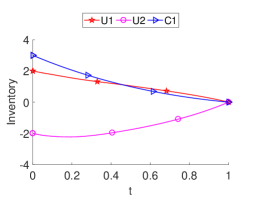
Figure 1. Depiction of the agents’ inventories in Section 6.1.

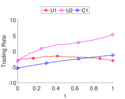
Figure 2. Depiction of the agents’ trading rates in Section 6.1.

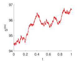
Figure 3. Depiction of the execution price in Section 6.1.

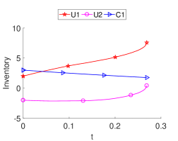
Figure 4. Depiction of the agents’ inventories in Section 6.2.

6.2. Example 2: A mini-flash crash with low trading volume

Our mini-flash crashes can be accompanied by low trading volumes (see Theorem 5.2). In Section 6.2, we visualize this by studying a concrete scenario in which $\det A$ has a root on $\left[0,T\right]$; $t_{e}>0$; the zero of $\det A$ at $t_{e}$ is of multiplicity 1; $\lambda\not\in\mathbb{Z}$; and $\lambda>0$. The behavior of the $X^{\theta_{j}^{\star}}_{j}\left(\omega\right)$’s is then characterized by Corollary 3.1 and Theorem 5.2. Theorem 5.2 would rigorously describe $S^{exc}_{t}\left(\omega\right)$ and the $\theta^{\star}_{j,t}\left(\omega\right)$’s as $t\uparrow t_{e}$, if $\lambda>1$. To improve the quality of our plots, we consider a situation where $\lambda\in\left(0,1\right)$ instead (see Remark 5.5).

By Lemmas 5.1 and 5.2, we must select parameters such that (5.1) is satisfied and

$$\lambda=\displaystyle\frac{2\left[\displaystyle\sqrt{\displaystyle\frac{\kappa}{\eta_{tem}}}\coth\left(\tau\left(t_{e}\right)\right)-2\left(\displaystyle\frac{K\tilde{\eta}_{per}-\eta_{per}}{K\tilde{\eta}_{tem}-\eta_{tem}}\right)\right]}{\left(K\tilde{\eta}_{tem}-\eta_{tem}\right)\dot{\Phi}\left(t_{e}\right)}$$ (6.9)

is a positive non-integer. We can keep most of our choices in (6.8) the same and only make a few revisions:

$$\begin{array}[]{lll}\tilde{\eta}_{tem}=0.5,&\eta_{tem}=0.2,&\tilde{\eta}_{per}=0.8,\\ \eta_{per}=0.025,&\nu^{2}=3,&\kappa=1.\end{array}$$ (6.12)

As in Section 6.1, we do not seek to replicate a particular historical situation. We immediately get (5.1), as its LHS is 4.3302. Using Remark 5.2 and (6.9), we can show that

$$t_{e}=0.2691\quad\text{and}\quad\lambda=0.5939.$$

Again, we have two uncertain agents and one certain agent. We retain the $\left\{U1,U2,C1\right\}$- labeling system from Section 6.1. The inventories, trading rates, and execution price are plotted in Figures 4 - 6. To aid our illustration, we truncate the time domains in Figures 5 - 6 to

$$\left[0,0.75\left(t_{e}-10^{-6}\right)\right]\quad\text{and}\quad\left[0,t_{e}-10^{-6}\right]$$

for the left and right plots, respectively.

The qualities that we expect based upon Theorem 5.2, and Remark 5.5 are all present. We offered some applicable comments in Section 6.1, so we only add a few new observations here.

1. All agents’ inventories approach a finite limit as $t\uparrow t_{e}$ (see Theorem 5.2 and Figure 4).

2. The execution price and the uncertain agents’ trading rates explode as $t\uparrow t_{e}$ (see Theorem 5.2, Remark 5.5 and Figures 5 - 6).

3. The uncertain agents’ trading rates synchronize as $t\uparrow t_{e}$ (see Theorem 5.2, Remark 5.5, and Figure 5).

4. That an explosion in $S^{exc}\left(\omega\right)$ will occur as well as its direction becomes increasingly obvious as $t\uparrow t_{e}$; however, it is not necessarily clear at first (see Theorem 5.2, Remark 5.5, and Figure 6).

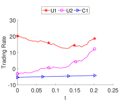
(a)

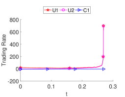
(b)

Figure 5. Depiction of the agents’ trading rates in Section 6.2.

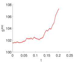
(a)

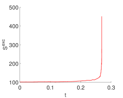
(b)

Figure 6. Depiction of the execution price in Section 6.2.

6.3. Example 3: A mini-flash crash with high trading volume

Our mini-flash crashes can also be accompanied by high trading volumes (see Theorem 5.1). We illustrate this in Section 6.3 by simulating a case in which $\det A$ has a root on $\left[0,T\right]$; $t_{e}>0$; the zero of $\det A$ at $t_{e}$ is of multiplicity 1; $\lambda\not\in\mathbb{Z}$; and $\lambda<0$. The behaviors of $S^{exc}\left(\omega\right)$, the $X^{\theta_{j}^{\star}}_{j}\left(\omega\right)$’s, and the $\theta^{\star}_{j}\left(\omega\right)$’s are then described by Corollary 3.1 and Theorem 5.1.

We especially wish to emphasize the stochastic explosion direction and do this in two ways.

First, we choose the same deterministic parameters to create Figures 7 - 12. The difference is that one realization of $\tilde{W}_{\cdot}$ is used in Figures 7 - 9, while another is used in Figures 10 - 12. We denote the corresponding $\omega$’s by $\omega_{up}$ and $\omega_{dn}$, since there are spikes and crashes in the former and latter plots, respectively.

Second, Figures 7 - 9 themselves suggest that the explosion direction is random. This is particularly true in Figures 8 - 9, since we initially notice that the price rapidly rises as the uncertain agents’ buying rates synchronize. Only moments before the mini-flash crash do we see the price collapsing and the uncertain agents’ aggressively selling together.

Now, we need to choose parameters such that (5.1) is satisfied and

$$\lambda=\displaystyle\frac{2\left[\displaystyle\sqrt{\displaystyle\frac{\kappa}{\eta_{tem}}}\coth\left(\tau\left(t_{e}\right)\right)-2\left(\displaystyle\frac{K\tilde{\eta}_{per}-\eta_{per}}{K\tilde{\eta}_{tem}-\eta_{tem}}\right)\right]}{\left(K\tilde{\eta}_{tem}-\eta_{tem}\right)\dot{\Phi}\left(t_{e}\right)}$$

is a negative non-integer due to Lemmas 5.1 and 5.1. Compared to Section 6.2, we set

$$\tilde{\eta}_{per}=0.5,\quad\eta_{per}=0.5$$

and keep every other parameter the same. As in Sections 6.1 - 6.2, we do not have in mind a special historical example here. Since we have only changed $\tilde{\eta}_{per}$ and $\eta_{per}$, the values of $\left(K\tilde{\eta}_{tem}-\eta_{tem}\right)\Phi\left(0\right)$ and $t_{e}$ do not differ from Section 6.2; however, $\lambda$ is now negative:

$$\left(K\tilde{\eta}_{tem}-\eta_{tem}\right)\Phi\left(0\right)=4.3302,\quad t_{e}=0.2691,\quad\text{and}\quad\lambda=-0.4531.$$

The numbers of uncertain and certain agents are still two and one, respectively. We also retain the $\left\{U1,U2,C1\right\}$-labeling system from Sections 6.1 - 6.2. Figures 7 and 10 depict the agents’ inventories. We plot the agents’ trading rates in Figures 8 and 11. The execution price appears in Figures 9 and 12. To help with our visualization, the time domains in the left plots in Figures 7 - 9 and Figures 10 - 12 are truncated to $\left[0,0.94\left(t_{e}-10^{-6}\right)\right]$ and $\left[0,0.75\left(t_{e}-10^{-6}\right)\right]$, respectively.

Our observations regarding Figures 7 - 12 are in agreement with Corollary 3.1 and Theorem 5.1. We have already made note of many important aspects in Sections 6.1 - 6.2 and only remark upon the new details.

1. The execution price, as well as the uncertain agents’ inventories and trading rates, all explode in the same direction as $t\uparrow t_{e}$ (see Theorem 5.1 and Figures 7 - 12).

2. The explosions take place at the deterministic time $t_{e}$ (see Theorem 5.1 and Figures 7 - 12).

3. The explosion direction depends on $\omega\in\tilde{\Omega}$ (see Theorem 5.1 and Figures 7 - 12).

4. The explosion direction cannot be known with complete certainty before $t_{e}$ (see Theorem 5.1 and Figures 7 - 12).

5. The explosion rates in the price and uncertain agents’ trading rates in Section 6.2 are slower than in Section 6.3 (see Figures 5 - 6, Figures 8 - 9, and Figures 11 - 12). We did not explicitly state this previously; however, this is to be expected since trading rates are integrable in Section 6.2 but not in Section 6.3.

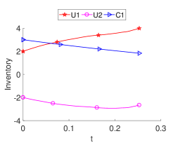
(a)

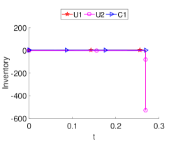
(b)

Figure 7. Depiction of the agents’ inventories for $\omega_{dn}$ in Section 6.3.

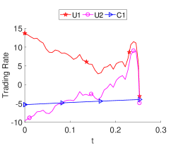
(a)

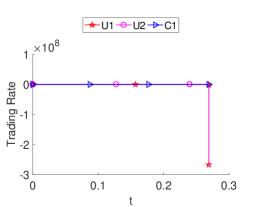
(b)

Figure 8. Depiction of the agents’ trading rates for $\omega_{dn}$ in Section 6.3.

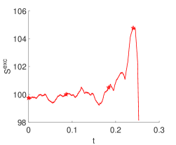
(a)

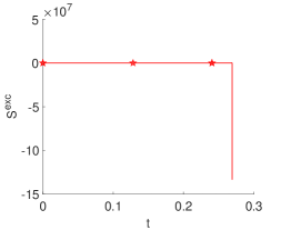
(b)

Figure 9. Depiction of the execution price for $\omega_{dn}$ in Section 6.3.

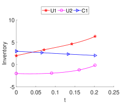
(a)

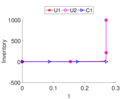
(b)

Figure 10. Depiction of the agents’ inventories for $\omega_{up}$ in Section 6.3.

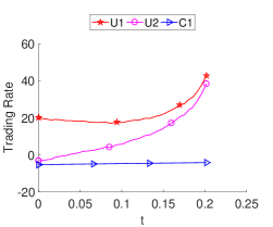
(a)

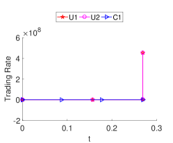
(b)

Figure 11. Depiction of the agents’ trading rates for $\omega_{up}$ in Section 6.3.

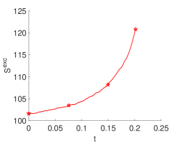
(a)

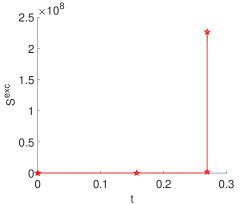
(b)

Figure 12. Depiction of the execution price for $\omega_{up}$ in Section 6.3.

7. conclusion

In this paper we show how mini-flash crashes might occur when agents learn and make their decisions based upon misspecified models. We give a necessary and sufficient condition for a mini-flash crash to occur and observe that if the agents

1. are too uncertain about their prior information

2. sufficiently underestimate the aggregate temporary impact

3. have long trading periods

4. have low risk aversion

then mini flash crashes occur.

Our numerical section has three main examples illustrating our three main results. In the first example, we see that not all human errors directly cause mini-flash crashes illustrating Proposition 4.2. Despite the regularity of the human errors on a market-wide basis, individual securities may rarely experience such an event. Similarly, traders’ models and strategies do roughly achieve their intended goals much of the time, as it is observed in the real markets.

The two other examples are about the nature of the mini-flash crashes. If a mini-flash crash does occur, it almost surely does so because of “endogenous triggering effects.” As predicted by Theorems 5.1 and 5.2), some of our agents also “converge on the same strategy” during mini-flash crashes: In certain cases, the agents driving these events all buy or sell together with the same (exploding) growth rate. The two theorems and the examples illustrating them are to demonstrate that mini-flash crashes can be accompanied by both high and low trading volumes.

Appendix A Section 3 Proofs

A.1. Proof of Lemma 3.1

Step 1: Denote the usual $P_{j}$-augmentation of $\left\{\mathcal{F}_{j,t}^{unf}\right\}_{0\leq t\leq T}$ by $\left\{\tilde{\mathcal{F}}_{j,t}^{unf}\right\}_{0\leq t\leq T}$. Let $\tilde{\mathcal{A}}_{j}$ be the space of $\tilde{\mathcal{F}}_{j,t}^{unf}$-progressively measurable processes $\theta_{j}$ such that (3.2) and (3.3) hold. We, again, define the process $X^{\theta_{j}}_{j}$ by (3.4) for any strategy $\theta_{j}\in\tilde{\mathcal{A}_{j}}$. Agent $j$’s auxiliary problem is to maximize

$$E^{P_{j}}\left[-\displaystyle\int_{0}^{T}\theta_{j,t}\,S_{j,\theta_{j},t}^{exc}\,dt-\displaystyle\frac{\kappa_{j}}{2}\displaystyle\int_{0}^{T}\left(X^{\theta_{j}}_{j,t}\right)^{2}\,dt\right]$$ (A.1)

over $\theta_{j}\in\tilde{\mathcal{A}}_{j}$. It is not difficult to show that

$$E^{P_{j}}\left[\beta_{j}\Big{|}\tilde{\mathcal{F}}_{j,t}^{unf}\right]=E^{P_{j}}\left[\beta_{j}\Big{|}\mathcal{F}_{j,t}^{unf}\right]\quad P_{j}-\text{a.s.}$$ (A.2)

Step 2: By (3.5) and (3.4),

$$-\displaystyle\int_{0}^{T}\theta_{j,t}\,S_{j,\theta_{j},t}^{exc}\,dt =-\displaystyle\int_{0}^{T}\theta_{j,t}\,S_{j,t}^{unf}\,dt-\displaystyle\int_{0}^{T}\theta_{j,t}\left[\eta_{j,per}\left(X_{j,t}^{\theta_{j}}-x_{j}\right)+\displaystyle\frac{1}{2}\eta_{j,tem}\theta_{j,t}\right]dt$$

for $\theta_{j}\in\tilde{\mathcal{A}}_{j}$. Section 7.4 of [34] and (3.1) imply that the process $\left\{\overline{W}_{j,t}\right\}_{0\leq t\leq T}$ with

$$\overline{W}_{j,t} \triangleq S_{j,t}^{unf}-S_{j,0}-\displaystyle\int_{0}^{t}E^{P_{j}}\left[\beta_{j}\big{|}\mathcal{F}_{j,s}^{unf}\right]\,ds$$

is an $\mathcal{F}_{j,t}^{unf}$-Wiener process under $P_{j}$ and

$$S_{j,t}^{unf}=S_{j,0}+\displaystyle\int_{0}^{t}E^{P_{j}}\left[\beta_{j}\big{|}\mathcal{F}_{j,s}^{unf}\right]\,ds+\overline{W}_{j,t}.$$ (A.3)

After integrating by parts and recalling (3.4) and (A.3), we get

$$E^{P_{j}}\left[-\displaystyle\int_{0}^{T}\theta_{j,t}\,S_{j,t}^{unf}\,dt\right]$$

$$\qquad=E^{P_{j}}\left[-X_{j,T}^{\theta_{j}}S_{j,T}^{unf}+\displaystyle\int_{0}^{T}X_{j,t}^{\theta_{j}}\,E^{P_{j}}\left[\beta_{j}\big{|}\mathcal{F}_{j,t}^{unf}\right]\,dt\right]+x_{j}S_{j,0}.$$

We also have

$$E^{P_{j}}\left[-\displaystyle\int_{0}^{T}\theta_{j,t}\left[\eta_{j,per}\left(X_{j,t}^{\theta_{j}}-x_{j}\right)+\displaystyle\frac{1}{2}\eta_{j,tem}\theta_{j,t}\right]dt\right]$$

$$\qquad=E^{P_{j}}\left[-\displaystyle\frac{1}{2}\eta_{j,per}\left(X_{j,T}^{\theta_{j}}-x_{j}\right)^{2}-\displaystyle\frac{1}{2}\eta_{j,tem}\displaystyle\int_{0}^{T}\theta_{j,t}^{2}\,dt\right].$$

Now $X_{j,T}^{\theta_{j}}=0$ $P_{j}$-a.s. by the definition of $\tilde{\mathcal{A}}_{j}$ in Step A.1. Since $x_{j}$, $S_{j,0}$ and $S_{j,T}^{unf}$ do not depend on Agent $j$’s choice of $\theta_{j}\in\tilde{\mathcal{A}}_{j}$, (A.2) implies that $\theta_{j}^{\star}$ maximizes (A.1) over $\theta_{j}\in\tilde{\mathcal{A}}_{j}$ if and only if it maximizes

$$E^{P_{j}}\left[\displaystyle\int_{0}^{T}X_{j,t}^{\theta_{j}}\,E^{P_{j}}\left[\beta_{j}\big{|}\tilde{\mathcal{F}}_{j,t}^{unf}\right]\,dt-\displaystyle\frac{1}{2}\eta_{j,tem}\displaystyle\int_{0}^{T}\theta_{j,t}^{2}\,dt-\displaystyle\frac{\kappa_{j}}{2}\displaystyle\int_{0}^{T}\left(X^{\theta_{j}}_{j,t}\right)^{2}\,dt\right].$$ (A.4)

Clearly, $\theta_{j}^{\star}$ maximizes (A.4) over $\theta_{j}\in\tilde{\mathcal{A}}_{j}$ if and only if it minimizes

$$E^{P_{j}}\left[\frac{1}{2}\displaystyle\int_{0}^{T}\left(X_{j,t}^{\theta_{j}}-\frac{E^{P_{j}}\left[\beta_{j}\big{|}\tilde{\mathcal{F}}_{j,t}^{unf}\right]}{\kappa_{j}}\right)^{2}\,dt+\displaystyle\frac{\eta_{j,tem}}{2\kappa_{j}}\displaystyle\int_{0}^{T}\theta_{j,t}^{2}\,dt\right].$$ (A.5)

Step 3: Recall the definition of $\tau_{j}(\cdot)$ from (3.7) and let

$$\begin{array}[]{ll}K_{j}\left(t,s\right)\triangleq\displaystyle\sqrt{\displaystyle\frac{\kappa_{j}}{\eta_{j,tem}}}\left(\displaystyle\frac{\sinh\left(\tau_{j}\left(s\right)\right)}{\cosh\left(\tau_{j}\left(t\right)\right)-1}\right),&\quad 0\leq t\leq s<T\\ &\\ \hat{\beta}_{j,t}\triangleq E^{P_{j}}\left[\displaystyle\frac{1}{\kappa_{j}}\left(1-\displaystyle\frac{1}{\cosh\left(\tau_{j}\left(t\right)\right)}\right)\right.&\\ &\\ \qquad\qquad\qquad\cdot\left.\displaystyle\int_{t}^{T}E^{P_{j}}\left[\beta_{j}\big{|}\tilde{\mathcal{F}}_{j,s}^{unf}\right]K_{j}\left(t,s\right)\,ds\,\Bigg{|}\,\tilde{\mathcal{F}}_{j,t}^{unf}\right],&\quad t\in\left[0,T\right).\end{array}$$ (A.11)

We see from Theorem 3.2 of [10] that (A.5) has a unique solution $\theta_{j}^{\star}\in\tilde{\mathcal{A}}_{j}$. Moreover, the corresponding optimal inventory process $X^{\theta^{\star}_{j}}_{j}$ satisfies the linear ODE

$$dX^{\theta^{\star}_{j}}_{j,t} =\displaystyle\sqrt{\displaystyle\frac{\kappa_{j}}{\eta_{j,tem}}}\coth\left(\tau_{j}\left(t\right)\right)\left(\hat{\beta}_{j,t}-X^{\theta^{\star}_{j}}_{j,t}\right)\,dt$$

$$X^{\theta^{\star}_{j}}_{j,0} =x_{j}$$ (A.12)

$dP_{j}\otimes dt$-a.s. on $\Omega_{j}\times\left[0,T\right)$.

Using Fubini’s theorem and (A.2), we get that

$$E^{P_{j}}\left[\displaystyle\int_{t}^{T}E^{P_{j}}\left[\beta_{j}\Big{|}\tilde{\mathcal{F}}_{j,s}^{unf}\right]K_{j}\left(t,s\right)\,ds\,\Bigg{|}\,\tilde{\mathcal{F}}_{j,t}^{unf}\right]=E^{P_{j}}\left[\beta_{j}\Big{|}\mathcal{F}_{j,t}^{unf}\right],\quad P_{j}-\text{a.s.}$$ (A.13)

The $\tanh$ half-angle formula together with (3.9) and (A.11) imply that (A.1) can be re-written as

$$\theta^{\star}_{j,t} =-\displaystyle\sqrt{\displaystyle\frac{\kappa_{j}}{\eta_{j,tem}}}\coth\left(\tau_{j}\left(t\right)\right)X^{\theta^{\star}_{j}}_{j,t}$$

$$\qquad+\displaystyle\frac{\tanh\left(\tau_{j}\left(t\right)/2\right)\left[\mu_{j}+\nu_{j}^{2}\left(S_{j,t}^{unf}-S_{j,0}\right)\right]}{\displaystyle\sqrt{\eta_{j,tem}\kappa_{j}}\left(1+\nu_{j}^{2}t\right)},\quad t\in\left(0,T\right)$$

$$X^{\theta^{\star}_{j}}_{j,0} =x_{j}.$$ (A.14)

Step 4: We know that $\theta^{\star}_{j}$ satisfies (3.2) and (3.3), as all strategies in $\tilde{\mathcal{A}}_{j}$ have these properties. Now $W_{j,\cdot}\left(\omega\right)$ is continuous on $\left[0,T\right]$ for $P_{j}$-almost every $\omega\in\Omega_{j}$. When such an $\omega$ is chosen, (A.1) becomes (3.1). The latter is a first order linear ODE with continuous coefficients, so $\theta^{\star}_{j,\cdot}\left(\omega\right)$ is continuous on $\left[0,T\right)$ (e.g., by Chapter 1.2 of [38]).

Since our terminal inventory constraint is deterministic, we observe that

$$\lim_{t\uparrow T}\theta^{\star}_{j,t}\left(\omega\right)$$

exists and is finite from (28) and (29) in the proof of Theorem 3.2 in [10], as well as (A.13) in Step A.1. In particular, we can view the paths of $\theta^{\star}_{j}$ on $\left[0,T\right]$ as $P_{j}$-a.s. continuous. We conclude by noting that $\theta_{j}^{\star}$ is also $\mathcal{F}_{j,t}^{unf}$-adapted by (28) and (29) in the proof of Theorem 3.2 in [10], (3.9), and (A.13) in Step A.1.

∎

Appendix B Section 4 Proofs

We frequently reference various easy properties of the functions in Definition 4.1. We collect these below for convenience. We will leave the proof to the reader.

Lemma B.1.

Fix $j\in\left\{1,\dots,K\right\}$. We have the following:

1. $\Phi_{j}$ is a strictly decreasing nonnegative function on $\left[0,T\right]$ with $\Phi_{j}\left(T\right)=0$.

2. The entries of $A$ are analytic on $\left[0,T\right]$ and $A\left(T\right)=I_{K}$.

3. If $\det A$ has a root on $\left[0,T\right]$, we can find the smallest one which we denote by $t_{e}$. In this case, $t_{e}<T$ and the zero of $\det A$ at $t_{e}$ is of finite multiplicity.

4. The entries of $B$ are analytic on $\left[0,T\right)$ but

   $$\lim_{t\uparrow T}B_{jj}\left(t\right)=-\infty.$$

5. $C\left(\cdot,\omega\right)$’s entries are continuous on $\left[0,T\right]$.

B.1. Proof of Lemma 4.1

Let $j\in\left\{1,\dots,K\right\}$. At each time $t$, Agent $j$ observes the correct value of $S_{t}^{exc}\left(\omega\right)$, interprets this value as the realized value of $S_{j,\theta_{j}^{\star},t}^{exc}\left(\omega\right)$, and computes $S_{j,t}^{unf}\left(\omega\right)$. By (3.5), it follows that

$$S_{t}^{exc}\left(\omega\right) =S_{j,\theta_{j}^{\star},t}^{exc}\left(\omega\right)$$

$$=S_{j,t}^{unf}\left(\omega\right)+\eta_{j,per}\left(X_{j,t}^{\theta_{j}^{\star}}\left(\omega\right)-x_{j}\right)+\frac{1}{2}\eta_{j,tem}\theta_{j,t}^{\star}\left(\omega\right).$$ (B.1)

After substituting (3.11) into (B.1), we have

$$S_{j,t}^{unf}\left(\omega\right)-S_{j,0}$$

$$\quad=\left(S_{0}-S_{j,0}\right)+\tilde{\beta}t+\displaystyle\sum_{\begin{subarray}{c}i\leq K\\ i\not=j\end{subarray}}\tilde{\eta}_{i,per}\left(X^{\theta_{i}^{\star}}_{i,t}\left(\omega\right)-x_{i}\right)+\displaystyle\sum_{i>K}\tilde{\eta}_{i,per}\left(X^{\theta_{i}^{\star}}_{i,t}-x_{i}\right)$$

$$\qquad+\frac{1}{2}\displaystyle\sum_{\begin{subarray}{c}i\leq K\\ i\not=j\end{subarray}}\tilde{\eta}_{i,tem}\theta_{i,t}^{\star}\left(\omega\right)+\frac{1}{2}\displaystyle\sum_{i>K}\tilde{\eta}_{i,tem}\theta_{i,t}^{\star}$$

$$\qquad+\left(\tilde{\eta}_{j,per}-\eta_{j,per}\right)\left(X_{j,t}^{\theta_{j}^{\star}}\left(\omega\right)-x_{j}\right)+\frac{1}{2}\left(\tilde{\eta}_{j,tem}-\eta_{j,tem}\right)\theta_{j,t}^{\star}\left(\omega\right)+\tilde{W}_{t}\left(\omega\right).$$ (B.2)

The quantity on the LHS of (B.1) plays a role in determining Agent $j$’s strategy (see Lemma 3.1). Substituting (B.1) into (3.1) and applying the half-angle formula for $\tanh\left(\cdot\right)$, we get

$$A_{jj}\left(t\right)\theta_{j,t}^{\star}\left(\omega\right)-\displaystyle\sum_{\begin{subarray}{c}i\leq K\\ i\not=j\end{subarray}}A_{ji}\left(t\right)\theta_{i,t}^{\star}\left(\omega\right)$$

$$\quad=B_{jj}\left(t\right)X^{\theta_{j}^{\star}}_{j,t}\left(\omega\right)+\displaystyle\sum_{\begin{subarray}{c}i\leq K\\ i\not=j\end{subarray}}B_{ji}\left(t\right)X^{\theta_{i}^{\star}}_{i,t}\left(\omega\right)+C_{j}\left(t,\omega\right).$$

It follows that the uncertain agents’ strategies are characterized by the ODE system

$$A\left(t\right)\theta_{t}^{u,\star}\left(\omega\right) =B\left(t\right)X^{u,\theta^{\star}}_{t}\left(\omega\right)+C\left(t,\omega\right)$$

$$X^{u,\theta^{\star}}_{0}\left(\omega\right) =x^{u}.$$ (B.3)

Corollary 3.1, Lemma B.1 and a standard existence and uniqueness theorem (see Sections 1.1 and 3.1 of [11]) finish the argument. ∎

B.2. Proof of Lemma 4.2

As $t\uparrow t_{e}$,

$$\begin{array}[]{c}\left\{A\left(t\right)\dot{X}_{t}^{u}\left(\omega\right)=B\left(t\right)X_{t}^{u}\left(\omega\right)\right\}\\ \iff\\ \left\{\left[\det A\left(t\right)\right]\dot{X}_{t}^{u}\left(\omega\right)=\left[\text{adj}A\left(t\right)\right]B\left(t\right)X_{t}^{u}\left(\omega\right)\right\}.\end{array}$$

Here, adj denotes the usual adjugate operator.

We can find a non-negative integer $m$ such that the multiplicity of the zero of $\det A$ at $t_{e}$ is $\left(m+1\right)$ by Lemma B.1. Hence, there is a unique non-vanishing analytic function $f$ such that

$$\det A\left(t\right)=\left(t-t_{e}\right)^{m+1}f\left(t\right)$$ (B.4)

on a small neighborhood of $t_{e}$. Note that $f$ is non-vanishing, as the zeroes of $\det A$ are isolated and $\det A\left(T\right)=1$ (see Lemma B.1). We then define the analytic (see Lemma B.1) map $D$ by

$$D\left(t\right)\triangleq\left[\text{adj}A\left(t\right)\right]B\left(t\right)/f\left(t\right)$$ (B.5)

and arrive at (4.3).

Since $\det A\left(\cdot\right)$ has a root at $t_{e}$, the rank of $A\left(t_{e}\right)$ is no more than $K-1$. We conclude by observing that adj $A\left(t_{e}\right)$ has rank 1 when $A\left(t_{e}\right)$ has rank $K-1$; otherwise, adj $A\left(t_{e}\right)$ must be the zero matrix. The comments about the rank of $D\left(t_{e}\right)$ immediately follow. ∎

B.3. Proof of Proposition 4.1

$D\left(t_{e}\right)\not=0$ since $\lambda\not=0$. Then (4) has a singular point of the first kind at $t_{e}$ (see our discussion above). $\lambda\not\in\mathbb{Z}$ by hypothesis, so Theorem 6.5 of [16] implies that a fundamental solution of (4) on $\left[t_{e}-\rho,t_{e}\right)$ for some $\rho>0$ is given by

$$P\left(t\right)\left|t-t_{e}\right|^{D\left(t_{e}\right)}.$$ (B.6)

In (B.6), $P\left(\cdot\right)$ is an analytic $M_{K}\left(\mathbb{R}\right)$-valued function with $P\left(t_{e}\right)=I_{K}$. Moreover, $P\left(t\right)$ is invertible for all $t\in\left[t_{e}-\rho,t_{e}\right)$ and

$$\left(P\left(t\right)\left|t-t_{e}\right|^{R}\right)^{-1}=\left|t-t_{e}\right|^{-R}\left[P\left(t\right)\right]^{-1}.$$ (B.7)

The solution of (4.1) satisfies

$$\left(t-t_{e}\right)\theta_{t}^{u,\star}\left(\omega\right) =D\left(t\right)X^{u,\theta^{\star}}_{t}\left(\omega\right)+\displaystyle\frac{\text{adj}\left[A\left(s\right)\right]C\left(s,\omega\right)}{f\left(s\right)}.$$

near $t_{e}$ (argue as in Lemma 4.2). Since

$$P\left(t\right)\left|t-t_{e}\right|^{D\left(t_{e}\right)}\rho^{-D\left(t_{e}\right)}\left[P\left(t_{e}-\rho\right)\right]^{-1}$$

is also a fundamental solution of (4.3) on $\left[t_{e}-\rho,t_{e}\right)$ and equals $I_{K}$ at $t_{e}-\rho$, we can apply variation of parameters to obtain

$$X^{u,\theta^{\star}}_{t}\left(\omega\right)$$

$$\,=P\left(t\right)\left|t-t_{e}\right|^{D\left(t_{e}\right)}\left[\rho^{-D\left(t_{e}\right)}\left[P\left(t_{e}-\rho\right)\right]^{-1}\right]\cdot\Bigg{[}X^{\theta^{\star}}_{t_{e}-\rho}\left(\omega\right)$$

$$\quad+\displaystyle\int_{t_{e}-\rho}^{t}\left(P\left(t_{e}-\rho\right)\rho^{D\left(t_{e}\right)}\left|s-t_{e}\right|^{-D\left(t_{e}\right)}\left[P\left(s\right)\right]^{-1}\right)\left(\displaystyle\frac{\text{adj}\left[A\left(s\right)\right]C\left(s,\omega\right)}{\left(s-t_{e}\right)f\left(s\right)}\right)ds\Bigg{]}.$$ (B.8)

We can find an eigenbasis $\left\{v_{1},\dots,v_{K}\right\}$ for $D\left(t_{e}\right)$ such that $v_{K}$ corresponds to $\lambda$. We then define the continuous real-valued functions $\left\{F_{1}\left(\cdot,\omega\right),\dots,F_{K}\left(\cdot,\omega\right)\right\}$ on $\left[t_{e}-\rho,t_{e}\right]$ and the constants $\left\{y_{1}\left(\omega\right),\dots,y_{K}\left(\omega\right)\right\}$ as certain eigenbasis coordinates:

$$\displaystyle\sum_{j=1}^{K}F_{j}\left(s,\omega\right)v_{j} \triangleq\displaystyle\frac{\left[P\left(s\right)\right]^{-1}\text{adj}\left[A\left(s\right)\right]C\left(s,\omega\right)}{f\left(s\right)}$$

$$\displaystyle\sum_{j=1}^{K}y_{j}\left(\omega\right)v_{j} \triangleq\rho^{-D\left(t_{e}\right)}\left[P\left(t_{e}-\rho\right)\right]^{-1}X^{\theta^{\star}}_{t_{e}-\rho}\left(\omega\right).$$ (B.9)

Taken with (B.3), these definitions immediately give (4.1) after recalling that for any matrix $Q\in M_{K}\left(\mathbb{R}\right)$ with eigenvalue $\gamma$ and corresponding eigenvector $v$, we have

$$\left|t-t_{e}\right|^{Q}v=\left|t-t_{e}\right|^{\gamma}v.$$

∎

B.4. Proof of Proposition 4.2

We know that $S^{exc}\left(\omega\right)$, the $X^{\theta_{j}^{\star}}_{j}\left(\omega\right)$’s and the $\theta^{\star}_{j}\left(\omega\right)$’s are all uniquely defined and continuous on $\left[0,T\right)$ (see Lemma 4.1). Corollary 3.1 implies that $X^{\theta_{j}^{\star}}_{j}\left(\omega\right)$ and $\theta^{\star}_{j}\left(\omega\right)$ are continuous at $T$ for $j>K$ (the certain agents). It also gives us

$$\lim_{t\uparrow T}X^{\theta_{j}^{\star}}_{j,t}\left(\omega\right)=0$$

for $j>K$. It remains to show that

$$\lim_{t\uparrow T}X^{u,\theta^{\star}}_{t}\left(\omega\right)=0\quad\text{and}\quad\displaystyle\lim_{t\uparrow T}\theta^{u,\star}_{t}\left(\omega\right)\in\mathbb{R}^{K}.$$ (B.10)

As discussed above, one difficulty is that the diagonal entries of $B$ in (4.1) explode at $T$ (see Lemma B.1); however, the approach for resolving this issue is similar to that used to analyze solution behavior near $t_{e}$.

First, we show that (4) (after replacing $t_{e}$ with $T$) has a singular point of the first kind at $T$. Now $\sinh\left(\tau_{j}\left(\cdot\right)\right)$ has a zero of multiplicity 1 at $T$ since

$$\frac{d\sinh\left(\tau_{j}\left(t\right)\right)}{dt}\Bigg{|}_{t=T}=-\displaystyle\sqrt{\displaystyle\frac{\kappa_{j}}{\eta_{j,tem}}}\cosh\left(\tau_{j}\left(t\right)\right)\Bigg{|}_{t=T}=-\displaystyle\sqrt{\displaystyle\frac{\kappa_{j}}{\eta_{j,tem}}}.$$

Hence, there is a unique non-vanishing analytic function $g_{j}$ such that

$$\sinh\left(\tau_{j}\left(t\right)\right)=\left(t-T\right)g_{j}\left(t\right)\quad\text{and}\quad g_{j}\left(T\right)=-\displaystyle\sqrt{\displaystyle\frac{\kappa_{j}}{\eta_{j,tem}}}$$ (B.11)

on a small neighborhood of $T$. Near $T$, it follows that the entries of $\left(t-T\right)B\left(t\right)$ are given by

$$\left(t-T\right)B_{ik}\left(t\right)=\left\{\begin{array}[]{ll}\left(t-T\right)\left(\tilde{\eta}_{i,per}-\eta_{i,per}\right)\Phi_{i}\left(t\right)&\\ \qquad-\displaystyle\sqrt{\displaystyle\frac{\kappa_{i}}{\eta_{i,tem}}}\left(\displaystyle\frac{\cosh\left(\tau_{i}\left(t\right)\right)}{g_{i}\left(t\right)}\right)&\quad\text{if }i=k\\ &\\ \left(t-T\right)\tilde{\eta}_{k,per}\Phi_{i}\left(t\right)&\quad\text{if }i\not=k\\ \end{array}\right.$$ (B.16)

(see Definition 4.1). On this region, the solution of (4) satisfies

$$\left(t-T\right)\dot{X}_{t}^{u}\left(\omega\right) =A^{-1}\left(t\right)\left(t-T\right)B\left(t\right)X_{t}^{u}\left(\omega\right).$$ (B.17)

By (B.16) and Lemma B.1, (B.17) has a singular point of the first kind at $T$.

Second, we find a fundamental solution of (B.17) near $T$. We know that

$$A^{-1}\left(T\right)=\left(t-T\right)B\left(t\right)\Bigg{|}_{t=T}=I_{K}$$

by (B.11), (B.16), and Lemma B.1. Theorem 6.5 of [16] implies that a fundamental solution of (B.17) on $\left[T-\delta,T\right)$ for some $\delta>0$ is given by

$$Q\left(t\right)\left|t-T\right|^{I_{K}}=Q\left(t\right)\left|t-T\right|.$$ (B.18)

In (B.18), $Q$ is an analytic $M_{K}\left(\mathbb{R}\right)$-valued function with $Q\left(T\right)=I_{K}$. Also, $Q\left(t\right)$ is invertible for all $t\in\left[T-\delta,T\right)$.

Finally, we use our fundamental solution to solve (4.1) and conclude the proof. Notice that $\tanh\left(\tau_{j}\left(\cdot\right)\right)$ also has a zero of multiplicity 1 at $T$ since

$$\frac{d\tanh\left(\tau_{j}\left(t\right)\right)}{dt}\Bigg{|}_{t=T}=-\displaystyle\frac{1}{2}\displaystyle\sqrt{\displaystyle\frac{\kappa_{j}}{\eta_{j,tem}}}\text{sech}^{2}\left(\tau_{j}\left(t\right)/2\right)\Bigg{|}_{t=T}=-\displaystyle\frac{1}{2}\displaystyle\sqrt{\displaystyle\frac{\kappa_{j}}{\eta_{j,tem}}}.$$

There is a unique non-vanishing analytic function $h_{j}$ such that

$$\tanh\left(\tau_{j}\left(t\right)/2\right)=\left(t-T\right)h_{j}\left(t\right)$$ (B.19)

on a neighborhood of $T$. In particular, the entries of $C\left(t,\omega\right)/\left(t-T\right)$ near $T$ are given by

$$\displaystyle\frac{C_{i}\left(t,\omega\right)}{\left(t-T\right)} =\left(\displaystyle\frac{h_{i}\left(t\right)\nu_{i}^{2}}{\sqrt{\eta_{i,tem}\kappa_{i}}\left(1+\nu_{i}^{2}t\right)}\right)\left[\displaystyle\frac{\mu_{i}}{\nu_{i}^{2}}+\left(S_{0}-S_{i,0}\right)+\tilde{\beta}t-\displaystyle\sum_{\begin{subarray}{c}k\leq K\\ k\not=i\end{subarray}}\tilde{\eta}_{k,per}x_{k}\right.$$

$$\qquad\qquad\qquad-x_{i}\left(\tilde{\eta}_{i,per}-\eta_{i,per}\right)+\displaystyle\sum_{k>K}\tilde{\eta}_{k,per}\left(X^{\theta_{k}^{\star}}_{k,t}-x_{k}\right)$$

$$\qquad\qquad\qquad\left.+\frac{1}{2}\displaystyle\sum_{k>K}\tilde{\eta}_{k,tem}\theta_{k,t}^{\star}+\tilde{W}_{t}\left(\omega\right)\right].$$ (B.20)

Since

$$Q\left(t\right)\left|t-T\right|\delta^{-1}Q^{-1}\left(T-\delta\right)$$

is also a fundamental solution of (4.3) on $\left[T-\delta,T\right)$ and equals $I_{K}$ at $T-\delta$, we can apply variation of parameters to obtain

$$X^{u,\theta^{\star}}_{t}\left(\omega\right)$$

$$\quad=Q\left(t\right)\left|t-T\right|\delta^{-1}Q^{-1}\left(T-\delta\right)\cdot\Bigg{[}X^{\theta^{\star}}_{T-\delta}\left(\omega\right)$$

$$\qquad+\displaystyle\int_{T-\delta}^{t}\left(Q\left(T-\delta\right)\delta\left|s-T\right|^{-1}Q^{-1}\left(s\right)\right)A^{-1}\left(s\right)C\left(s,\omega\right)ds\Bigg{]}.$$ (B.21)

By (B.4), (B.4), and Corollary 3.1, we get (B.10). ∎

Appendix C Section 5 Proofs

C.1. Proof of Lemma 5.1

First observe that (5.1) is equivalent to

$$\left(K\tilde{\eta}_{tem}-\eta_{tem}\right)\Phi\left(0\right)>2,$$ (C.1)

by Definitions 3.7 and 4.1. By Definitions 4.1 and 5.1, we see that $A$ is now given by

$$A_{ik}\left(t\right) \triangleq\left\{\begin{array}[]{cc}1-\displaystyle\frac{1}{2}\left(\tilde{\eta}_{tem}-\eta_{tem}\right)\Phi\left(t\right)&\quad\text{if }i=k\\ -\displaystyle\frac{1}{2}\tilde{\eta}_{tem}\Phi\left(t\right)&\quad\text{if }i\not=k\\ \end{array}\right..$$ (C.4)

A short calculation shows that

$$\det A\left(t\right) =\left[1+\displaystyle\frac{1}{2}\eta_{tem}\Phi\left(t\right)\right]^{K-1}\left[1-\displaystyle\frac{1}{2}\left(K\tilde{\eta}_{tem}-\eta_{tem}\right)\Phi\left(t\right)\right].$$ (C.5)

The first term in (C.5) is always at least 1. The second term is non-zero at 0 but does have a root on $\left(0,T\right]$ if and only if (C.1) holds. Both of these observations come from Lemma B.1.

Now, (C.1) implies that $K\tilde{\eta}_{tem}>\eta_{tem}$. Since $t_{e}$ is a zero of $\det A$, we must have that

$$1-\displaystyle\frac{1}{2}\left(K\tilde{\eta}_{tem}-\eta_{tem}\right)\Phi\left(t_{e}\right)=0.$$ (C.6)

Hence, by Lemma B.1,

$$\displaystyle\frac{d\left[\det A\left(t\right)\right]}{dt}\Bigg{|}_{t=t_{e}} =-\displaystyle\frac{1}{2}\left(K\tilde{\eta}_{tem}-\eta_{tem}\right)\left[1+\displaystyle\frac{1}{2}\eta_{tem}\Phi\left(t\right)\right]^{K-1}\dot{\Phi}\left(t\right)\Bigg{|}_{t=t_{e}}>0.$$ (C.7)

∎

C.2. Proof of Lemma 5.2

By (B.4), (C.7), and Lemma 5.1,

$$f\left(t_{e}\right) =\displaystyle\frac{d\left[\det A\left(t\right)\right]}{dt}\Bigg{|}_{t=t_{e}}$$

$$=-\displaystyle\frac{1}{2}\left(K\tilde{\eta}_{tem}-\eta_{tem}\right)\left[1+\displaystyle\frac{1}{2}\eta_{tem}\Phi\left(t_{e}\right)\right]^{K-1}\dot{\Phi}\left(t_{e}\right).$$ (C.8)

A short calculation shows that adj $A\left(t\right)$ is given by

$$\left[\text{adj}A\left(t\right)\right]_{ik}$$

$$=\left(1+\displaystyle\frac{1}{2}\eta_{tem}\Phi\left(t\right)\right)^{K-2}\left\{\begin{array}[]{ll}1-\displaystyle\frac{1}{2}\left[\left(K-1\right)\tilde{\eta}_{tem}-\eta_{tem}\right]\Phi\left(t\right)&\quad\text{if }i=k\\ \displaystyle\frac{1}{2}\tilde{\eta}_{tem}\Phi\left(t\right)&\quad\text{if }i\not=k\\ \end{array}\right..$$ (C.11)

It follows that

$$\left[\left(\text{adj}A\left(t\right)\right]B\left(t\right)\right]_{ik}$$

$$\quad=\tilde{\eta}_{per}\Phi\left(t\right)\left(1+\displaystyle\frac{1}{2}\eta_{tem}\Phi\left(t\right)\right)^{K-1}$$

$$\qquad+\left(1+\displaystyle\frac{1}{2}\eta_{tem}\Phi\left(t\right)\right)^{K-2}\left(\eta_{per}\Phi\left(t\right)+\displaystyle\sqrt{\displaystyle\frac{\kappa}{\eta_{tem}}}\coth\left(\tau\left(t\right)\right)\right)$$

$$\qquad\qquad\cdot\left\{\begin{array}[]{ll}\displaystyle\frac{1}{2}\left[\left(K-1\right)\tilde{\eta}_{tem}-\eta_{tem}\right]\Phi\left(t\right)-1&\quad\text{if }i=k\\ &\\ -\displaystyle\frac{1}{2}\tilde{\eta}_{tem}\Phi\left(t\right)&\quad\text{if }i\not=k\\ \end{array}\right..$$ (C.15)

One can then check that the only potentially non-zero eigenvalue of

$$D\left(t_{e}\right)=\displaystyle\frac{\left[\text{adj}A\left(t_{e}\right)\right]B\left(t_{e}\right)}{f\left(t_{e}\right)}$$

is given by

$$\lambda =-\displaystyle\frac{2\left[\left(K\tilde{\eta}_{per}-\eta_{per}\right)\Phi\left(t_{e}\right)-\displaystyle\sqrt{\displaystyle\frac{\kappa}{\eta_{tem}}}\coth\left(\tau\left(t_{e}\right)\right)\right]}{\left(K\tilde{\eta}_{tem}-\eta_{tem}\right)\dot{\Phi}\left(t_{e}\right)}$$ (C.16)

with corresponding eigenvector $v_{K}$ as above. We get (5.3) from (C.16) after applying (5.2).

Recall that $\Phi\left(t_{e}\right)>0$ and $\dot{\Phi}\left(t_{e}\right)<0$ by Lemma B.1. Since $t_{e}$, $\Phi$, and $\tau$ do not depend on $\tilde{\eta}_{per}$ or $\eta_{per}$, we can ensure that $\lambda\not\in\mathbb{Z}$ by perturbing the latter parameters. $D\left(t_{e}\right)$ is then diagonalizable as observed in Proposition 4.1, and $v_{1},\dots,v_{K-1}$ can be computed using (C.2). ∎

C.3. Proof of Theorems 5.1 and 5.2

Since our uncertain agents are semi-symmetric,

$$C_{i}\left(t,\omega\right) =\Phi\left(t\right)\tilde{W}_{t}\left(\omega\right)$$

$$\qquad+\Phi\left(t\right)\left[\tilde{\beta}t+\displaystyle\sum_{k>K}\tilde{\eta}_{k,per}\left(X^{\theta_{k}^{\star}}_{k,t}-x_{k}\right)+\frac{1}{2}\displaystyle\sum_{k>K}\tilde{\eta}_{k,tem}\theta_{k,t}^{\star}\right]$$

$$\qquad+\Phi\left(t\right)\left[\displaystyle\frac{\mu_{i}}{\nu^{2}}+\left(S_{0}-S_{i,0}\right)-\displaystyle\sum_{\begin{subarray}{c}k\leq K\\ k\not=i\end{subarray}}\tilde{\eta}_{per}x_{k}-x_{i}\left(\tilde{\eta}_{per}-\eta_{per}\right)\right]$$ (C.17)

for $t\leq t_{e}$ by Definition 4.1. For convenience, we introduce the following deterministic function $c$ and the constants $c_{1},\dots,c_{K}$:

$$c\left(t\right) \triangleq\left[\tilde{\beta}t+\displaystyle\sum_{k>K}\tilde{\eta}_{k,per}\left(X^{\theta_{k}^{\star}}_{k,t}-x_{k}\right)+\frac{1}{2}\displaystyle\sum_{k>K}\tilde{\eta}_{k,tem}\theta_{k,t}^{\star}\right]$$

$$\displaystyle\sum_{i=1}^{K}c_{i}v_{i} \triangleq\left[\begin{array}[]{c}\displaystyle\frac{\mu_{1}}{\nu^{2}}+\left(S_{0}-S_{1,0}\right)-\displaystyle\sum_{\begin{subarray}{c}k\leq K\\ k\not=1\end{subarray}}\tilde{\eta}_{per}x_{k}-x_{1}\left(\tilde{\eta}_{per}-\eta_{per}\right)\\ \vdots\\ \displaystyle\frac{\mu_{K}}{\nu^{2}}+\left(S_{0}-S_{K,0}\right)-\displaystyle\sum_{\begin{subarray}{c}k\leq K\\ k\not=K\end{subarray}}\tilde{\eta}_{per}x_{k}-x_{K}\left(\tilde{\eta}_{per}-\eta_{per}\right)\end{array}\right].$$ (C.21)

Using (C.3), we get that

$$C\left(t,\omega\right) =\tilde{W}_{t}\left(\omega\right)\Phi\left(t\right)v_{K}+c\left(t\right)\Phi\left(t\right)v_{K}+\Phi\left(t\right)\displaystyle\sum_{i=1}^{K}c_{i}v_{i}.$$ (C.22)

By (C.2), $\left\{v_{1},\dots,v_{K}\right\}$ is an eigenbasis for $\text{adj}\left[A\left(t\right)\right]$. Moreover,

$$\left(1+\displaystyle\frac{1}{2}\eta_{tem}\Phi\left(t\right)\right)^{K-2}\left[1-\displaystyle\frac{1}{2}\left(K\tilde{\eta}_{tem}-\eta_{tem}\right)\Phi\left(t\right)\right]$$ (C.23)

is the eigenvalue corresponding to each of $v_{1},\dots,v_{K-1}$, while

$$\left(1+\displaystyle\frac{1}{2}\eta_{tem}\Phi\left(t\right)\right)^{K-1}$$ (C.24)

corresponds to $v_{K}$.

By (B.3), it follows that

$$\displaystyle\sum_{j=1}^{K}F_{j}\left(t,\omega\right)v_{j}$$

$$\quad=\displaystyle\frac{\left[P\left(t\right)\right]^{-1}\text{adj}\left[A\left(t\right)\right]C\left(t,\omega\right)}{f\left(t\right)}$$

$$\quad=\tilde{W}_{t}\left(\omega\right)\left(\displaystyle\frac{\Phi\left(t\right)\left(1+\displaystyle\frac{1}{2}\eta_{tem}\Phi\left(t\right)\right)^{K-1}}{f\left(t\right)}\right)\left[P\left(t\right)\right]^{-1}v_{K}$$

$$\qquad\quad+\left(\displaystyle\frac{\Phi\left(t\right)\left(1+\displaystyle\frac{1}{2}\eta_{tem}\Phi\left(t\right)\right)^{K-1}\left(c\left(t\right)+c_{K}\right)}{f\left(t\right)}\right)\left[P\left(t\right)\right]^{-1}v_{K}$$

$$\qquad\quad+\left(\displaystyle\frac{\Phi\left(t\right)\left(1+\displaystyle\frac{1}{2}\eta_{tem}\Phi\left(t\right)\right)^{K-2}\left[1-\displaystyle\frac{1}{2}\left(K\tilde{\eta}_{tem}-\eta_{tem}\right)\Phi\left(t\right)\right]}{f\left(t\right)}\right)$$

$$\qquad\qquad\qquad\cdot\displaystyle\sum_{i=1}^{K-1}c_{i}\left[P\left(t\right)\right]^{-1}v_{i}.$$ (C.25)

It follows that we can find analytic deterministic functions $F_{j,1}$ and $F_{j,2}$ such that

$$F_{j}\left(t,\omega\right)\triangleq\tilde{W}_{t}\left(\omega\right)F_{j,1}\left(t\right)+F_{j,2}\left(t\right)$$ (C.26)

for each $j\in\left\{1,\dots,K\right\}$. Since $P\left(t_{e}\right)=I_{K}$ (see Proposition 4.1), (C.2) and Remark 5.2 further imply that

$$F_{j,1}\left(t_{e}\right)=F_{j,2}\left(t_{e}\right)=\cdots=F_{K-1,1}\left(t_{e}\right)=F_{K-1,2}\left(t_{e}\right)=0$$ (C.27)

and

$$F_{K,1}\left(t_{e}\right)=-\displaystyle\frac{\Phi^{2}\left(t_{e}\right)}{\dot{\Phi}\left(t_{e}\right)}>0\quad\text{and}\quad F_{K,2}\left(t_{e}\right)=-\displaystyle\frac{\Phi^{2}\left(t_{e}\right)}{\dot{\Phi}\left(t_{e}\right)}\left(c\left(t_{e}\right)+c_{K}\right).$$ (C.28)

While $F_{K,1}\left(t_{e}\right)>0$, determining the sign of $F_{K,2}\left(t_{e}\right)$ is difficult, in general, as it depends upon the sign of $c\left(t_{e}\right)+c_{K}$ (see (C.3)).

We see from (C.26) and (C.27) that the expression

$$\frac{F_{j}\left(s,\omega\right)}{\left|s-t_{e}\right|}$$ (C.29)

is bounded near $t_{e}$ for each $j<K$ and almost every $\omega\in\tilde{\Omega}$. In particular, the coordinates of both

$$\sum_{j=1}^{K-1}\left(y_{j}\left(\omega\right)-\displaystyle\int_{t_{e}-\rho}^{t}\displaystyle\frac{F_{j}\left(s,\omega\right)}{\left|s-t_{e}\right|}\,ds\right)P\left(t\right)v_{j}$$

and its time derivative are bounded near $t_{e}$ for such $\omega$ as well.

Since $P\left(t_{e}\right)=I_{K}$, the $v_{K}$-coordinate of $P\left(t\right)v_{K}$ tends to 1 $t\uparrow t_{e}$. For $j<K$, the $v_{j}$-coordinate of $P\left(t\right)v_{K}$ tends to 0 as $t\uparrow t_{e}$. In each situation, we can also obtain Lipschitz bounds on the convergence. Due to (4.1) and (C.26), potential explosions in the coordinates of $X^{u,\theta^{\star}}_{t}\left(\omega\right)$ are characterized by

$$\lim_{t\uparrow t_{e}}\left[\left|t-t_{e}\right|^{\lambda}\left(y_{K}\left(\omega\right)-\displaystyle\int_{t_{e}-\rho}^{t}\displaystyle\frac{\tilde{W}_{s}\left(\omega\right)F_{K,1}\left(s\right)+F_{K,2}\left(s\right)}{\left|s-t_{e}\right|^{1+\lambda}}\,ds\right)\right].$$ (C.30)

Specifically,

$$\left\{\left|\text{(\ref{Xu explosion last integral eqn SCALAR})}\right|<+\infty\right\}\quad \iff\quad\left\{\displaystyle\lim_{t\uparrow t_{e}}X^{u,\theta^{\star}}_{t}\left(\omega\right)\quad\text{exists in }\mathbb{R}^{K}\right\}$$

$$\left\{\text{(\ref{Xu explosion last integral eqn SCALAR})}=+\infty\right\}\quad \iff\quad\left\{\displaystyle\lim_{t\uparrow t_{e}}X^{u,\theta^{\star}}_{t}\left(\omega\right)=\left[+\infty,\dots,+\infty\right]^{\top}\right\}$$

$$\left\{\text{(\ref{Xu explosion last integral eqn SCALAR})}=-\infty\right\}\quad \iff\quad\left\{\displaystyle\lim_{t\uparrow t_{e}}X^{u,\theta^{\star}}_{t}\left(\omega\right)=\left[-\infty,\dots,-\infty\right]^{\top}\right\}.$$ (C.31)

To finish the proof, we separately consider the $\lambda<0$ and $\lambda>0$ cases.

$\lambda<0$ Case.

Assume that $\lambda<0$. It follows that

$$\lim_{t\uparrow t_{e}}\displaystyle\int_{t_{e}-\rho}^{t}\displaystyle\frac{\left|\tilde{W}_{s}\left(\omega\right)F_{K,1}\left(s\right)\right|}{\left|s-t_{e}\right|^{1+\lambda}}\,ds<\infty\quad\text{and}\quad\displaystyle\lim_{t\uparrow t_{e}}\displaystyle\int_{t_{e}-\rho}^{t}\displaystyle\frac{\left|F_{K,2}\left(s\right)\right|}{\left|s-t_{e}\right|^{1+\lambda}}\,ds<\infty.$$

Clearly,

$$\lim_{t\uparrow t_{e}}\left|t-t_{e}\right|^{\lambda}=+\infty,$$

meaning that

$$\left\{y_{K}\left(\omega\right)-\displaystyle\lim_{t\uparrow t_{e}}\displaystyle\int_{t_{e}-\rho}^{t}\displaystyle\frac{F_{K,2}\left(s\right)}{\left|s-t_{e}\right|^{1+\lambda}}\,ds>\displaystyle\lim_{t\uparrow t_{e}}\displaystyle\int_{t_{e}-\rho}^{t}\displaystyle\frac{\tilde{W}_{s}\left(\omega\right)F_{K,1}\left(s\right)}{\left|s-t_{e}\right|^{1+\lambda}}\,ds\right\}$$ (C.32)

$$\quad\implies\quad\left\{\displaystyle\lim_{t\uparrow t_{e}}X^{u,\theta^{\star}}_{t}\left(\omega\right)=\left[+\infty,\dots,+\infty\right]^{\top}\right\}$$

and

$$\left\{y_{K}\left(\omega\right)-\displaystyle\lim_{t\uparrow t_{e}}\displaystyle\int_{t_{e}-\rho}^{t}\displaystyle\frac{F_{K,2}\left(s\right)}{\left|s-t_{e}\right|^{1+\lambda}}\,ds<\displaystyle\lim_{t\uparrow t_{e}}\displaystyle\int_{t_{e}-\rho}^{t}\displaystyle\frac{\tilde{W}_{s}\left(\omega\right)F_{K,1}\left(s\right)}{\left|s-t_{e}\right|^{1+\lambda}}\,ds\right\}$$ (C.33)

$$\quad\implies\quad\left\{\displaystyle\lim_{t\uparrow t_{e}}X^{u,\theta^{\star}}_{t}\left(\omega\right)=\left[-\infty,\dots,-\infty\right]^{\top}\right\}$$

Arguing as in our discussion of (C.29), we see that the hypotheses in (C.32) and (C.33) also imply that

$$\left\{\displaystyle\lim_{t\uparrow t_{e}}\theta^{u,\star}_{t}\left(\omega\right)=\left[+\infty,\dots,+\infty\right]^{\top}\right\}\quad\text{and}\quad\left\{\displaystyle\lim_{t\uparrow t_{e}}\theta^{u,\star}_{t}\left(\omega\right)=\left[-\infty,\dots,-\infty\right]^{\top}\right\},$$

respectively. Conditional on $\tilde{\mathcal{F}}_{t_{e}-\rho}$, the RHS of the inequality in (C.32) (and C.33) is deterministic. Since $F_{K,1}\left(t_{e}\right)>0$ (see (C.28)), we finish our proof of Theorem 5.1.

$\lambda>0$ Case.

Assume that $\lambda>0$. We can find a constant $R_{0}\left(\omega\right)$ such that

$$\left|y_{K}\left(\omega\right)-\displaystyle\int_{t_{e}-\rho}^{t}\displaystyle\frac{\tilde{W}_{s}\left(\omega\right)F_{K,1}\left(s\right)+F_{K,2}\left(s\right)}{\left|s-t_{e}\right|^{1+\lambda}}\,ds\right|\leq\displaystyle\frac{R_{0}\left(\omega\right)}{\left|t-t_{e}\right|^{\lambda}}.$$ (C.34)

Hence, (C.30) is bounded as $t\uparrow t_{e}$ and

$$\lim_{t\uparrow t_{e}}X^{u,\theta^{\star}}_{t}\left(\omega\right)$$

exists in $\mathbb{R}^{K}$ by our previous comments.

By our discussion surrounding (C.29), we see that explosions in the coordinates of $\theta^{u,\star}_{t}\left(\omega\right)$ are characterized by

$$\displaystyle\lim_{t\uparrow t_{e}} \left[-\lambda\left|t-t_{e}\right|^{\lambda-1}\left(y_{K}\left(\omega\right)-\displaystyle\int_{t_{e}-\rho}^{t}\displaystyle\frac{\tilde{W}_{s}\left(\omega\right)F_{K,1}\left(s\right)+F_{K,2}\left(s\right)}{\left|s-t_{e}\right|^{1+\lambda}}\,ds\right)\right.$$

$$\qquad\left.-\left(\displaystyle\frac{\tilde{W}_{t}\left(\omega\right)F_{K,1}\left(t\right)+F_{K,2}\left(t\right)}{\left|t-t_{e}\right|}\right)\right].$$ (C.35)

More precisely,

$$\left\{\text{(\ref{lamb pos theta expl key term 1})}=+\infty\right\}\quad \iff\quad\left\{\displaystyle\lim_{t\uparrow t_{e}}\theta^{u,\star}_{t}\left(\omega\right)=\left[+\infty,\dots,+\infty\right]^{\top}\right\}$$

$$\left\{\text{(\ref{lamb pos theta expl key term 1})}=-\infty\right\}\quad \iff\quad\left\{\displaystyle\lim_{t\uparrow t_{e}}\theta^{u,\star}_{t}\left(\omega\right)=\left[-\infty,\dots,-\infty\right]^{\top}\right\}.$$ (C.36)

Suggestively, we first rewrite the expression in (C.3) as

$$F_{K,2}\left(t\right)\left(\lambda\left|t-t_{e}\right|^{\lambda-1}\displaystyle\int_{t_{e}-\rho}^{t}\displaystyle\frac{1}{\left|s-t_{e}\right|^{1+\lambda}}\,ds-\displaystyle\frac{1}{\left|t-t_{e}\right|}\right)$$

$$\quad+\lambda\left|t-t_{e}\right|^{\lambda-1}\displaystyle\int_{t_{e}-\rho}^{t}\displaystyle\frac{F_{K,2}\left(s\right)-F_{K,2}\left(t\right)}{\left|s-t_{e}\right|^{1+\lambda}}\,ds$$

$$\quad-\lambda\left|t-t_{e}\right|^{\lambda-1}y_{K}\left(\omega\right)$$

$$\quad+\tilde{W}_{t}\left(\omega\right)F_{K,1}\left(t\right)\left(\lambda\left|t-t_{e}\right|^{\lambda-1}\displaystyle\int_{t_{e}-\rho}^{t}\displaystyle\frac{1}{\left|s-t_{e}\right|^{1+\lambda}}\,ds-\displaystyle\frac{1}{\left|t-t_{e}\right|}\right)$$

$$\quad+\lambda\left|t-t_{e}\right|^{\lambda-1}\displaystyle\int_{t_{e}-\rho}^{t}\displaystyle\frac{\tilde{W}_{s}\left(\omega\right)\left[F_{K,1}\left(s\right)-F_{K,1}\left(t\right)\right]}{\left|s-t_{e}\right|^{1+\lambda}}\,ds$$

$$\quad+\lambda\left|t-t_{e}\right|^{\lambda-1}F_{K,1}\left(t\right)\displaystyle\int_{t_{e}-\rho}^{t}\displaystyle\frac{\tilde{W}_{s}\left(\omega\right)-\tilde{W}_{t}\left(\omega\right)}{\left|s-t_{e}\right|^{1+\lambda}}\,ds$$ (C.37)

Let $R_{1}$ and $R_{2}$ be the deterministic Lipschitz coefficients for $F_{K,1}$ and $F_{K,2}$. The first two lines of (C.3) are deterministic, and we can obtain the following bounds:

$$\begin{split}&\left|F_{K,2}\left(t\right)\left(\lambda\left|t-t_{e}\right|^{\lambda-1}\displaystyle\int_{t_{e}-\rho}^{t}\displaystyle\frac{1}{\left|s-t_{e}\right|^{1+\lambda}}\,ds-\displaystyle\frac{1}{\left|t-t_{e}\right|}\right)\right|\\ &\qquad\leq\displaystyle\frac{\left|F_{K,2}\left(t\right)\right|\left|t-t_{e}\right|^{\lambda-1}}{\rho^{\lambda}}\\ &\left|\lambda\left|t-t_{e}\right|^{\lambda-1}\displaystyle\int_{t_{e}-\rho}^{t}\displaystyle\frac{F_{K,2}\left(s\right)-F_{K,2}\left(t\right)}{\left|s-t_{e}\right|^{1+\lambda}}\,ds\right|\\ &\qquad\leq\left(\displaystyle\frac{\lambda R_{2}}{1-\lambda}\right)\left(\rho^{1-\lambda}\left|t-t_{e}\right|^{\lambda-1}-1\right)\end{split}$$

In (C.3), the third line is deterministic conditional on $\tilde{\mathcal{F}}_{t_{e}-\rho}$. Lines 4 - 6 of (C.3) are stochastic conditional on $\tilde{\mathcal{F}}_{t_{e}-\rho}$. Letting $R_{3}\left(\omega\right)$ be the maximum of $\left|\tilde{W}_{t}\left(\omega\right)\right|$ on $\left[t_{e}-\rho,t_{e}\right]$, we notice that

$$\begin{split}&\left|\tilde{W}_{t}\left(\omega\right)F_{K,1}\left(t\right)\left(\lambda\left|t-t_{e}\right|^{\lambda-1}\displaystyle\int_{t_{e}-\rho}^{t}\displaystyle\frac{1}{\left|s-t_{e}\right|^{1+\lambda}}\,ds-\displaystyle\frac{1}{\left|t-t_{e}\right|}\right)\right|\\ &\qquad\leq\displaystyle\frac{F_{K,1}\left(t\right)\left|\tilde{W}_{t}\left(\omega\right)\right|\left|t-t_{e}\right|^{\lambda-1}}{\rho^{\lambda}}\\ &\left|\lambda\left|t-t_{e}\right|^{\lambda-1}\displaystyle\int_{t_{e}-\rho}^{t}\displaystyle\frac{\tilde{W}_{s}\left(\omega\right)\left[F_{K,1}\left(s\right)-F_{K,1}\left(t\right)\right]}{\left|s-t_{e}\right|^{1+\lambda}}\,ds\right|\\ &\qquad\leq\left(\displaystyle\frac{\lambda R_{1}R_{3}\left(\omega\right)}{1-\lambda}\right)\left(\rho^{1-\lambda}\left|t-t_{e}\right|^{\lambda-1}-1\right).\end{split}$$

When $\lambda>1$, it follows that we see that (C.3) has the same behavior as

$$\lim_{t\uparrow t_{e}}\left[\left|t-t_{e}\right|^{\lambda-1}\displaystyle\int_{t_{e}-\rho}^{t}\displaystyle\frac{\tilde{W}_{s}\left(\omega\right)-\tilde{W}_{t}\left(\omega\right)}{\left|s-t_{e}\right|^{1+\lambda}}\,ds\right]$$ (C.38)

(all other terms tend to 0 $\tilde{P}$-a.s.). Using integration by parts,

$$\left|t-t_{e}\right|^{\lambda-1}\displaystyle\int_{t_{e}-\rho}^{t}\displaystyle\frac{\tilde{W}_{s}\left(\omega\right)-\tilde{W}_{t}\left(\omega\right)}{\left|s-t_{e}\right|^{1+\lambda}}\,ds$$

$$\qquad\sim\mathcal{N}\left(0,\left|t-t_{e}\right|^{2\lambda-2}\displaystyle\int_{t_{e}-\rho}^{t}\left(\displaystyle\frac{\left|s-t_{e}\right|^{-\lambda}}{\lambda}-\displaystyle\frac{1}{\lambda\rho^{\lambda}}\right)^{2}ds\right).$$ (C.39)

Asymptotically, the variance in (C.3) grows like $\left|t-t_{e}\right|^{-1}$ as $t\uparrow t_{e}$, completing the proof of Theorem 5.2. ∎

References

• [1] BBC News: probe into Japan share sale error. http://news.bbc.co.uk/2/hi/business/4512962.stm. Accessed: 2017-04-15.
• [2] Commodity Futures Trading Commission and the Securities & Exchange Commission: findings regarding the market events of May 6, 2010. https://www.sec.gov/news/studies/2010/marketevents-report.pdf. Accessed: 2017-04-15.
• [3] Nanex LLC.: flash crash summary report. http://www.nanex.net/FlashCrashFinal/FlashCrashSummary.html. Accessed: 2017-04-15.
• [4] Nanex LLC.: NxResearch. http://www.nanex.net/NxResearch/. Accessed: 2017-04-15.
• [5] Securities and Exchange Commission: Merrill Lynch charged with trading control failures that led to mini flash crashes. https://www.sec.gov/news/pressrelease/2016-192.html. Accessed: 2017-04-15.
• [6] R. Almgren and N. Chriss, Value under liquidation, Risk, 12 (1999), pp. 61–63.
• [7]  , Optimal execution of portfolio transactions, J. Risk, 3 (2001), pp. 5–40.
• [8] R. Almgren and J. Lorenz, Adaptive arrival price, Trading, 2007 (2007), pp. 59–66.
• [9] R. F. Almgren, Optimal execution with nonlinear impact functions and trading-enhanced risk, Appl. Math. Finance, 10 (2003), pp. 1–18.
• [10] P. Bank, H. M. Soner, and M. Voß, Hedging with temporary price impact, Math. Financ. Econ., 11 (2017), pp. 215–239.
• [11] V. Barbu, Differential equations, Springer Undergraduate Mathematics Series, Springer, Cham, 2016. Translated from the 1985 Romanian original by Liviu Nicolaescu.
• [12] P. Cardaliaguet and C.-A. Lehalle, Mean field game of controls and an application to trade crowding, Mathematics and Financial Economics, 12 (2018), pp. 335–363.
• [13] B. I. Carlin, M. S. Lobo, and S. Viswanathan, Episodic liquidity crises: cooperative and predatory trading, J. Finance, 62 (2007), pp. 2235–2274.
• [14] Á. Cartea, S. Jaimungal, and D. Kinzebulatov, Algorithmic trading with learning, Int. J. Theoretical Appl. Finance, 19 (2016), p. 1650028.
• [15] P. Casgrain and S. Jaimungal, Algorithmic Trading with Partial Information: A Mean Field Game Approach, ArXiv e-prints, (2018).
• [16] E. A. Coddington and R. Carlson, Linear ordinary differential equations, Society for Industrial and Applied Mathematics (SIAM), Philadelphia, PA, 1997.
• [17] K. Colaneri, Z. Eksi, R. Frey, and M. Szölgyenyi, Shall I sell or shall I wait? Optimal liquidation under partial information with price impact, ArXiv e-prints, (2016).
• [18] D. Dick, Erroneous combustion, CFA Institute Magazine, 24 (2013), pp. 20–21.
• [19] D. Easley, M. M. López de Prado, and M. O‘Hara, Flow toxicity and liquidity in a high-frequency world, Rev. Financ. Stud., 25 (2012), p. 1457.
• [20] D. Easley, M. M. López de Prado, and M. O’Hara, The microstructure of the “flash crash”: flow toxicity, liquidity crashes, and the probability of informed trading, J. Portfolio Manage., 37 (2011), pp. 118–128.
• [21] E. Ekström and J. Vaicenavicius, Optimal liquidation of an asset under drift uncertainty, SIAM J. Financial Math., 7 (2016), pp. 357–381.
• [22] M. Farrell, Mini flash crashes: a dozen a day. http://money.cnn.com/2013/03/20/investing/mini-flash-crash/. Accessed: 2017-04-15.
• [23] V. Filimonov and D. Sornette, Quantifying reflexivity in financial markets: Toward a prediction of flash crashes, Phys. Rev. E., 85 (2012), p. 056108.
• [24] R. Frey, A. Gabih, and R. Wunderlich, Portfolio optimization under partial information with expert opinions, Int. J. Theor. Appl. Finance, 15 (2012), p. 1250009.
• [25] N. Gârleanu and L. H. Pedersen, Dynamic trading with predictable returns and transaction costs, J. Finance, 68 (2013), pp. 2309–2340.
• [26] R. Gayduk and S. Nadtochiy, Liquidity Effects of Trading Frequency, Math. Finance, (forthcoming).
• [27] A. Golub, J. Keane, and S.-H. Poon, High frequency trading and mini flash crashes, ArXiv e-prints, (2012).
• [28] J. Huang and J. Wang, Liquidity and market crashes, Rev. Financ. Stud, 22 (2009), pp. 2607–2643.
• [29] N. I. Ismail and L. Mnyanda, Flash crash of the pound baffles traders with algorithms being blamed. https://www.bloomberg.com/news/articles/2016-10-06/pound-plunges-6-1-percent-in-biggest-drop-since-brexit-result. Accessed: 2017-04-15.
• [30] S. J. Leal, M. Napoletano, A. Roventini, and G. Fagiolo, Rock around the clock: An agent-based model of low- and high-frequency trading, J. Evol. Econ., 26 (2016), pp. 49–76.
• [31] N. Johnson, G. Zhao, E. Hunsader, H. Qi, N. Johnson, J. Meng, and B. Tivnan, Abrupt rise of new machine ecology beyond human response time, Sci. Rep., 3 (2013), pp. 1–7.
• [32] A. Joulin, A. Lefevre, D. Grunberg, and J.-P. Bouchaud, Stock price jumps: news and volume play a minor role, Wilmott Magazine, Sep/Oct (2008), pp. 1–7.
• [33] A. A. Kirilenko, A. S. Kyle, M. Samadi, and T. Tuzun, The flash crash: high frequency trading in an electronic market, J. Finance, (forthcoming).
• [34] R. S. Liptser and A. N. Shiryaev, Statistics of random processes. I, vol. 5 of Applications of Mathematics (New York), Springer-Verlag, Berlin, expanded ed., 2001. General theory, Translated from the 1974 Russian original by A. B. Aries, Stochastic Modelling and Applied Probability.
• [35] S. Mamudi, Sudden stock crashes usually caused by human error, SEC says. https://www.bloomberg.com/news/articles/2013-06-18/sudden-stock-crashes-mostly-show-human-error-sec-s-berman-says. Accessed: 2017-04-15.
• [36] F. Passerini and S. E. Vazquez, Optimal trading with alpha predictors, ArXiv e-prints, (2015).
• [37] J. A. Scheinkman and W. Xiong, Overconfidence and speculative bubbles, J. Polit. Econ., 111 (2003), pp. 1183–1220.
• [38] W. Walter, Ordinary differential equations, vol. 182 of Graduate Texts in Mathematics, Springer-Verlag, New York, 1998. Translated from the sixth German (1996) edition by Russell Thompson, Readings in Mathematics.