Bulk viscosity of two-flavor quark matter from the Kubo formalism

Abstract

We study the bulk viscosity of quark matter in the strong coupling regime within the two-flavor Nambu–Jona-Lasinio model. The dispersive effects that lead to nonzero bulk viscosity arise from quark-meson fluctuations above the Mott transition temperature, where meson decay into two quarks is kinematically allowed. We adopt the Kubo-Zubarev formalism and compute the equilibrium imaginary-time correlation function for pressure in the $O(1/N_{c})$ power counting scheme. The bulk viscosity of matter is expressed in terms of the Lorentz components of the quark spectral function and includes multiloop contributions which arise via resummation of infinite geometrical series of loop diagrams. We show that the multiloop contributions dominate the single-loop contribution close to the Mott line, whereas at high temperatures the one-loop contribution is dominant. The multiloop bulk viscosity dominates the shear viscosity close to the Mott temperature by factors 5 to 20, but with increasing temperature the shear viscosity becomes the dominant dissipation mechanism of stresses as the one-loop contribution becomes the main source of bulk viscosity.

I Introduction

The transport coefficients of quark-gluon plasma continue to attract significant attention as they are key inputs in the hydrodynamical description of heavy-ion collisions at the energies of the Relativistic Heavy Ion Collider (RHIC) and Large Hadron Collider (LHC). The data on elliptic flow in the heavy-ion collisions can be well described by a low value of the shear viscosity $\eta$ of the fluid, with the ratio of the shear viscosity to the entropy density $s$ being close to the lower bound placed by the uncertainty principle 1985PhRvD..31…53D and conjectured from AdS/CFT duality arguments 2005PhRvL..94k1601K .

The role of the bulk viscosity, which describes the dissipation in the case where pressure falls out of equilibrium on uniform expansion or contraction of a statistical ensemble, is more subtle. As it is well known, bulk viscosity vanishes in a number of cases, e.g., for ultrarelativistic and nonrelativistic gases interacting weakly with local forces via binary collisions LIFSHITZ19811 ; 1971ApJ…168..175W .

The bulk viscosity $\zeta$ of quark-gluon plasma is small in the perturbative regime 1985NuPhB.250..666H ; 2006PhRvD..74h5021A ; 2008JHEP…09..015M ; 2013PhRvD..87c6002C , but was found to be large close to the critical temperature of the chiral phase transition. For example, lattice simulations of the pure gluodynamcis close the critical temperature predict $\zeta/s\sim 1$ 2008PhRvL.100p2001M , where $s$ is the entropy density, and it is expected that $\zeta$ becomes singular at the critical point of second order phase transition 2006PhRvC..74a4901P . Values of $\zeta/s\sim 1$ affect the description of data in heavy-ion collisions 2012PhRvC..85d4909D and can lead to a breakdown of the fluid description via onset of cavitation 2010JHEP…03..018R .

Controlled computations of the bulk viscosity exist in perturbative QCD on the basis of kinetic theory of relativistic quarks 2006PhRvD..74h5021A ; 2008JHEP…09..015M ; 2013PhRvD..87c6002C . In the strongly coupled regime various approximate methods were applied, including QCD sum rules in combination with the lattice data on the QCD equation state 2008JHEP…09..015M ; 2008PhLB..663..217K ; Aarts:2007va and quasiparticle Boltzmann transport 2010NuPhA.832…62S ; 2011PhRvC..83a4906C ; 2011PhRvD..84i4025C ; 2012EPJC…72.1873D ; Marty:2013ita . Some strongly coupled systems can exhibit zero bulk viscosity if the scale or, more generally, the conformal symmetry is intact. This is the case, for example, in atomic Fermi gases in the unitary limit 2006PhRvA..74e3604W ; 2007PhRvL..98b0604S ; 2011AnPhy.326..770E ; 2013PhRvL.111l0603D , but not in the QCD and QCD-inspired theories when the conformal symmetry is broken by the quark mass terms and/or by dimensionful regularization of the ultraviolet divergences. This is indeed the case in the Nambu–Jona-Lasinio (NJL) model of low-energy QCD that we will utilize below.

A nonperturbative method to compute the transport coefficients of quark-gluon plasma close to the chiral phase transition is based on the Kubo-Zubarev formalism 1957JPSJ…12..570K ; zubarev1997statistical , with the correlators computed from the quark spectral function derived from the NJL model in conjunction with the $1/N_{c}$ diagrammatic expansion 1994PhRvC..49.3283Q . This approach has been applied extensively to compute the shear viscosity of quark plasma 2008JPhG…35c5003I ; 2008EPJA…38…97A ; LW14 ; LKW15 ; LangDiss ; 2016PhRvC..93d5205G , but there exist only a few computations of the bulk viscosity 2014ChPhC..38e4101X ; 2016PhRvC..93d5205G in this regime.

In this work we extend the previous study of the transport coefficients of two-flavor quark mater within the Kubo-Zubarev formalism and NJL model 2017arXiv170204291H to compute the bulk viscosity of quark plasma close to the critical line of the chiral phase transition. We specifically argue that the one-loop result for the correlation function of quarks, which arises in the leading order of $1/N_{c}$ expansion, cannot be applied in the case of bulk viscosity and a resummation of infinite series is required. As a consequence, our results are substantially different from those obtained previously from the one-loop computations.

For completeness we point out that the bulk viscosity of dense and cold QCD was extensively discussed in the context of compact stars and strange stars because it is the dominant dissipation mechanism to damp the unstable Rossby waves ($r$-modes)  2007PhRvC..75e5209A ; 2007PhRvD..75f5016S ; 2007PhRvD..75l5004S ; 2007PhRvD..75g4016D ; 2008JPhG…35k5007A ; 2010PhRvD..81d5015H ; 2011NJPh…13d5018S ; 2016PhRvD..94l3010B . In this regime of QCD the bulk viscosity is dominated by the weak interaction process like $\beta$-decays of quarks $d\to u+e+\bar{\nu}$ or nonleptonic weak process in three-flavor quark matter $u+d\to u+s$. The time scales associated with the weak processes are much larger than the collisional time scale. The situation is an analogue of the case of bulk viscosity of fluids undergoing chemical reactions on time scales much larger than the collisional time scale, which may lead to large bulk viscosity, as shown long ago by Mandelstam and Leontovich ML . This contribution to the bulk viscosity is called “soft-mode” contribution, because it is described by the response of the system to small frequency perturbations 2015PhRvC..91b5805K . As we are interested here in the hydrodynamical description of heavy-ion collisions, which have characteristic time-scales much shorter than the weak time scale, we will not discuss weak processes. Slow “chemical equilibration” processes may play a role in the bulk viscosity in the multicomponent environment in heavy-ion collisions, but are beyond the scope of this work.

The paper is organized as follows. Section II starts from the Kubo-Zubarev formula for the bulk viscosity and expresses it in terms of the Lorentz components of the quark spectral function. In Sec. III we summarize the results of Ref. 2017arXiv170204291H for the quark spectral function, in the case where the dispersive effects arise from the quark-meson fluctuations. Our numerical results for the bulk viscosity are collected in Sec. IV. Section V provides a short summary of our results. Appendix A describes the details of the computation of the bulk viscosity beyond one-loop approximation. In Appendix B we discuss the thermodynamics of the model and derive a number of relations that are required for the computation of the bulk viscosity. We use the natural (Gaussian) units with $\hbar=c=k_{B}=1$, and the metric signature $(1,-1,-1,-1)$.

II Kubo formula for bulk viscosity

We consider two-flavor quark matter described by the NJL-Lagrangian of the form

$$\mathcal{L}=\bar{\psi}(i\not{\partial}-m_{0})\psi+\frac{G}{2}\left[(\bar{\psi}\psi)^{2}+(\bar{\psi}i\gamma_{5}\bm{\tau}\psi)^{2}\right],$$ (1)

where $\psi=(u,d)^{T}$ is the iso-doublet quark field, $m_{0}=5.5$ MeV is the current-quark mass, $G=10.1$ GeV^-2 is the effective four-fermion coupling constant and $\bm{\tau}$ is the vector of Pauli isospin matrices. This Lagrangian describes four-fermion contact scalar-isoscalar and pseudoscalar-isovector interactions between quarks with the corresponding bare vertices $\Gamma^{0}_{s}=1$ and $\Gamma^{0}_{ps}=i\bm{\tau}\gamma_{5}$. The symmetrized energy momentum tensor is given in the standard fashion by

$$T_{\mu\nu}=\frac{i}{2}(\bar{\psi}\gamma_{\mu}\partial_{\nu}\psi+\bar{\psi}\gamma_{\nu}\partial_{\mu}\psi)-g_{\mu\nu}\mathcal{L}.$$ (2)

The net particle current is given by

$$N_{\mu}=\bar{\psi}\gamma_{\mu}\psi,$$ (3)

which is the only conserved current in the case of isospin-symmetric quark matter, i.e., quark matter described by a single chemical potential for both flavors.

The Kubo and Zubarev formalisms relate the transport properties of material to different types of equilibrium correlation functions of an ensemble zubarev1997statistical ; 1957JPSJ…12..570K , which in turn can be computed from equilibrium many-body techniques.

The bulk (second) viscosity within the Kubo-Zubarev formalism is given by 1987NuPhB.280..716H ; 2011AnPhy.326.3075H

$$\zeta=-\frac{d}{d\omega}\rm{Im}\Pi^{R}_{\zeta}(\omega)\bigg{|}_{\omega=0},$$ (4)

where the relevant two-point correlation function is given by

$$\Pi^{R}_{\zeta}(\omega)=-i\int_{0}^{\infty}dt\ e^{i\omega t}\int d\bm{r}\langle\left[\hat{p}^{*}(\bm{r},t),\hat{p}^{*}(0)\right]\rangle_{0},$$ (5)

with

$$\hat{p}^{*}(\bm{r},t) = \hat{p}(\bm{r},t)-\gamma\hat{\epsilon}(\bm{r},t)-\delta\hat{n}(\bm{r},t)$$ (6)

$$= \frac{1}{3}T_{ii}(\bm{r},t)-\gamma T_{00}(\bm{r},t)-\delta N_{0}(\bm{r},t).$$

Here $\hat{p}$, $\hat{\epsilon}$ and $\hat{n}$ are operators of the pressure, the energy density and the particle number density, respectively; the second line uses the relation between these quantities and energy-momentum tensor and particle number current in the fluid rest frame; $\gamma$ and $\delta$ are thermodynamic quantities and are given by

$$\gamma=\bigg{(}\frac{\partial p}{\partial\epsilon}\bigg{)}_{n},\quad\delta=\bigg{(}\frac{\partial p}{\partial n}\bigg{)}_{\epsilon}.$$ (7)

The last term in Eq. (6) is present only at finite chemical potentials; see Appendix B for details.

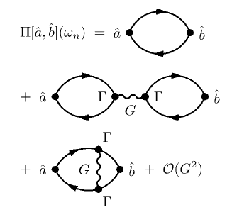
Figure 1: Contributions to the two-point correlation functions from ${\cal O}(N_{c}^{1})$ (first and second lines) and ${\cal O}(N_{c}^{0})$ (the third line) diagrams which are either of zeroth or first order in the coupling constant $G$.

Inserting Eq. (6) into Eq. (5) we obtain a set of two-point correlation functions of the generic form

$$\Pi[\hat{a},\hat{b}](\omega_{n})=\int_{0}^{\beta}\!\!d\tau e^{i\omega_{n}\tau}\int d\bm{r}\langle{\cal T}_{\tau}(\bar{\psi}\hat{a}\psi\Big{|}_{(\bm{r},\tau)},\bar{\psi}\hat{b}\psi\Big{|}_{0})\rangle_{0},$$

where we switched to the imaginary-time Matsubara formalism by means of the substitutions $t\to-i\tau$, $\partial_{t}\to i\partial_{\tau}$. In Eq. (II) $\omega_{n}=2\pi nT$, $n=0,\pm 1,\ldots$ is a bosonic Matsubara frequency with $T$ being the temperature of the system, ${\cal T}_{\tau}$ is the imaginary time-ordering operator and

$\hat{a}$ and $\hat{b}$ stand for either a differential operator (contracted with Dirac $\gamma$-matrices) or an interaction vertex $\Gamma^{0}_{s/ps}$ appearing in Eqs. (1)–(3).

The required retarded correlation functions can be obtained from Eq. (II) by an analytic continuation $i\omega_{n}\to\omega+i\delta$. The procedure of computation of the bulk viscosity is slightly more involved than that of the conductivities and shear viscosity 2008JPhG…35c5003I ; 2008EPJA…38…97A ; LW14 ; LKW15 ; LangDiss ; 2016PhRvC..93d5205G because the single-loop approximation to Eq. (II) does not cover all the relevant diagrams in the $1/N_{c}$ expansion. Figure 1 shows the $G^{0}$ and $G^{1}$ order terms of diagrammatic expansion for the two-point correlation function given by Eq. (II). To select the leading-order diagrams in the $1/N_{c}$ power-counting scheme, the following rules are applied: (i) each loop contributes a factor of $N_{c}$ from the trace over color space; (ii) each coupling $G$ associated with a pair of $\Gamma^{0}_{s/ps}$ matrices contributes a factor of $1/N_{c}$ 1994PhRvC..49.3283Q ; 2008JPhG…35c5003I ; 2008EPJA…38…97A ; LW14 ; LKW15 ; 2016PhRvC..93d5205G ; LangDiss . Applying these rules we conclude that the diagrams in the first and the second lines in Fig. 1 are of order of $N_{c}$. The third diagram, which is a first-order vertex correction, is of order of $N_{c}^{0}$, and, therefore, is suppressed compared to the previous ones. Thus, the correlation function (II) in the leading [${\cal O}(N_{c}^{1})$] order is given by an infinite sum of bubble diagrams, each of which consists of several single-loop diagrams. The latter in the momentum space is given by (see the first line in Fig. 1)

$$\Pi_{0}[\hat{a},\hat{b}](\omega_{n}) \equiv -T\sum_{l}\!\!\int\!\!\frac{d{\bm{p}}}{(2\pi)^{3}}$$ (9)

$$\times {\rm Tr}\left[\hat{a}G({\bm{p}},i\omega_{l}+i\omega_{n})\hat{b}G({\bm{p}},i\omega_{l})\right].$$

Here $G({\bm{p}},i\omega_{l})$ is the dressed Matsubara quark-antiquark propagator, the summation goes over fermionic Matsubara frequencies $\omega_{l}=\pi(2l+1)T-i\mu$, $l=0,\pm 1,\ldots,$ with $\mu$ being the chemical potential, and $\hat{a}$ and $\hat{b}$ are the momentum-space counterparts of the same operators appearing in Eq. (II). The traces should be taken in Dirac, color, and flavor space. The details of these computations and the loop resummation are relegated to Appendix A.

To express the correlation functions given by Eq. (9) in terms of the Lorentz components of the spectral function we write the full quark retarded/advanced Green’s function as

$$G^{R/A}(p_{0},\bm{p})=\frac{1}{\not{p}-m-\Sigma^{R/A}(p_{0},\bm{p})},$$ (10)

where $m$ is the constituent quark mass, $\Sigma^{R/A}$ in (10) is the quark retarded/advanced self-energy which is written in terms of its Lorentz components as

$$\Sigma^{R(A)}=m\Sigma_{s}^{(*)}-p_{0}\gamma_{0}\Sigma_{0}^{(*)}+\bm{p}\bm{\gamma}\Sigma_{v}^{(*)}.$$ (11)

By definition, the spectral function is given by

$$A(p_{0},\bm{p}) = -\frac{1}{2\pi i}[G^{R}(p_{0},\bm{p})-G^{A}(p_{0},\bm{p})]$$ (12)

$$= -\frac{1}{\pi}(mA_{s}+p_{0}\gamma_{0}A_{0}-\bm{p}\bm{\gamma}A_{v}),$$

where the scalar $A_{s}$, temporal $A_{0}$ and vector $A_{v}$ components are expressed through combinations of the components (real and imaginary) of the self-energy according to the relations LKW15 ; 2017arXiv170204291H

$$A_{i}(p_{0},p)=\frac{1}{d}[n_{1}\varrho_{i}-2n_{2}(1+r_{i})],\quad d=n_{1}^{2}+4n_{2}^{2},$$ (13)

with

$$n_{1} = p_{0}^{2}[(1+r_{0})^{2}-\varrho_{0}^{2}]$$ (14)

$$- \bm{p}^{2}[(1+r_{v})^{2}-\varrho_{v}^{2}]-m^{2}[(1+r_{s})^{2}-\varrho_{s}^{2}],$$

$$n_{2} = p_{0}^{2}\varrho_{0}(1+r_{0})$$ (15)

$$- \bm{p}^{2}\varrho_{v}(1+r_{v})-m^{2}\varrho_{s}(1+r_{s}),$$

where we used the shorthand notations $\varrho_{i}={\rm Im}\Sigma_{i}$ and $r_{i}={\rm Re}\Sigma_{i}$, $i=s,0,v$. From now on we will neglect the irrelevant real parts of the self-energy, which lead to momentum-dependent corrections to the constituent quark mass in next-to-leading order ${\cal O}(N_{c}^{-1})$.

The bulk viscosity in terms of the components of the spectral function is then written as

$$\zeta=\zeta_{0}+\zeta_{1}+\zeta_{2},$$ (16)

with the one-loop contribution given by

$$\zeta_{0} = -\frac{2N_{c}N_{f}}{9\pi^{3}}\int_{-\infty}^{\infty}d\varepsilon\frac{\partial n}{\partial\varepsilon}\int_{0}^{\Lambda}dpp^{2}\Big{[}2(ax+by+cz)^{2}$$ (17)

$$-(x^{2}-y^{2}+z^{2})(a^{2}-b^{2}+c^{2})\Big{]},$$

where $N_{c}=3$ and $N_{f}=2$ are the color and flavor numbers, respectively, and

$$x=3(1+\gamma)m_{0},\quad y=3(\delta-\varepsilon),\quad z=(2+3\gamma)p,$$ (18)

$$a=mA_{s},\quad b=\varepsilon A_{0},\quad c=pA_{v}.$$ (19)

In Eq. (17) we introduced a regularizing 3-momentum ultraviolet cutoff $\Lambda$; below we adopt the value $\Lambda=0.65$ GeV. The quark distribution function is given by

$$n(\varepsilon)=\frac{1}{e^{\beta(\varepsilon-\mu)}+1},$$ (20)

with $\beta=T^{-1}$ being the inverse temperature. The following two contributions in Eq. (16) are given by

$$\zeta_{1}=2(\bar{G}\bar{R})I_{1},\qquad\zeta_{2}=(\bar{G}\bar{R})^{2}I_{2},$$ (21)

where the renormalized coupling $\bar{G}$ arises through resummation of geometrical series as

$$\bar{G}=\frac{G}{1-R_{0}G},$$ (22)

with the polarization loop

$$R_{0} = -\frac{2N_{c}N_{f}}{\pi^{4}}\int_{-\infty}^{\infty}d\varepsilon\int_{-\infty}^{\infty}d\varepsilon^{\prime}\frac{n(\varepsilon)-n(\varepsilon^{\prime})}{\varepsilon-\varepsilon^{\prime}}$$ (23)

$$\times\int_{0}^{\Lambda}dpp^{2}(aa^{\prime}+bb^{\prime}-cc^{\prime}).$$

Finally, the three functions appearing in Eq. (21) are given by

$$I_{1} = -\frac{2N_{c}N_{f}}{3\pi^{3}}\int_{-\infty}^{\infty}d\varepsilon\frac{\partial n}{\partial\varepsilon}\int_{0}^{\Lambda}dpp^{2}$$ (24)

$$\times\Big{[}x(a^{2}+b^{2}-c^{2})+2a(by+cz)\Big{]},$$

$$I_{2} = -\frac{2N_{c}N_{f}}{\pi^{3}}\int_{-\infty}^{\infty}d\varepsilon\frac{\partial n}{\partial\varepsilon}\int_{0}^{\Lambda}dpp^{2}(a^{2}+b^{2}-c^{2}),$$ (25)

$$\bar{R} = -\frac{2N_{c}N_{f}}{3\pi^{4}}\int_{-\infty}^{\infty}d\varepsilon\int_{-\infty}^{\infty}d\varepsilon^{\prime}\int_{0}^{\Lambda}dp{p^{2}}\frac{1}{\varepsilon-\varepsilon^{\prime}}$$ (26)

$$\times \Big{\{}[n(\varepsilon)-n(\varepsilon^{\prime})]\big{[}x(aa^{\prime}+bb^{\prime}-cc^{\prime})+z(a^{\prime}c+ac^{\prime})\big{]}$$

$$+\Big{[}yn(\varepsilon)-y^{\prime}n(\varepsilon^{\prime})+\frac{3}{2}(\varepsilon-\varepsilon^{\prime})\Big{]}(a^{\prime}b+ab^{\prime})\Big{\}}.$$

Here the functions $a^{\prime},b^{\prime},c^{\prime},y^{\prime}$ are obtained from $a,b,c,y$ defined in Eqs. (18) and (19) by substitution $\varepsilon\to\varepsilon^{\prime}$. Equations (16)–(26) express the bulk viscosity of the quark plasma in terms of the components of its spectral function.

It is remarkable that the multiloop contributions do not vanish if the chiral symmetry is explicitly broken. However, in the chiral limit $m_{0}=0$ they vanish trivially, since quarks become massless above the critical temperature $T_{c}$ (see the next section). Indeed, from Eqs. (18) and (19) we find $x=0$ and $a,a^{\prime}\propto m=0$ in this case. Consequently, it follows from Eqs. (26) and (21) that $\zeta_{1,2}=0$. Therefore, the bulk viscosity in this case is given by the single-loop contribution $\zeta_{0}$, which remains finite also in the chiral limit; see also the discussion in Sec. IV.3.

III Phase diagram and spectral functions

Here we specify the structure of the phase diagram of strongly interacting quark matter and review the processes that lead to the dispersive effects (imaginary parts of the self-energy of quarks and antiquarks) within the region of $\mu$-$T$ plain. Our discussion is based on the two-flavor NJL model described by the Lagrangian (1).

Within the NJL model the nonzero temperature and density constituent quark mass is determined to leading order in the $1/N_{c}$ expansion from a Dyson-Schwinger equation, where the self-energy is taken in the Hartree approximation in terms of a tadpole diagram (so called quark condensate), see Fig. 2. From Fig. 2 we obtain the following equation for the constituent quark mass

$$m=m_{0}-G\langle\bar{\psi}\psi\rangle,$$ (27)

where the quark condensate is given by

$$\langle\bar{\psi}\psi\rangle=-\frac{mN_{c}N_{f}}{\pi^{2}}\int_{0}^{\Lambda}dp\frac{p^{2}}{E_{p}}[1-n^{+}(E_{p})-n^{-}(E_{p})],$$

with quark/antiquark thermal distributions $n^{\pm}(E)=[e^{\beta(E\mp\mu)}+1]^{-1}$.

The propagators of $\pi$ and $\sigma$ mesons are found from the Bethe-Salpeter equation illustrated in Fig. 3, which resums contributions from quark-antiquark polarization insertions.

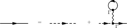
Figure 2: The Dyson-Schwinger equation for the constituent quark mass. The dashed and solid lines stand for the bare and dressed propagators, respectively, and the vertex $\Gamma=1$. The wavy line represents the interaction.

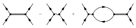
Figure 3: The Bethe-Salpeter equation for mesons: the double lines stand for the dressed meson propagators. The remaining diagrammatic elements are as in Fig. 2, except that the vertex assumes the values $\Gamma^{0}_{s}=1$ for $\sigma$ meson and $\Gamma^{0}_{ps}=i\bm{\tau}\gamma_{5}$ for pions.

Once the in-medium propagator of mesons is found, their masses are then determined from the propagator poles in real spacetime for $\bm{p}=0$; for details see 2017arXiv170204291H and references therein.

The region of the $\mu$-$T$ plain where our model is applicable is shown in Fig. 4 by the shaded area. Its outer boundary is given by the maximal temperature $T_{\rm max}$ above which no solutions for meson masses can be found. More precisely, mesonic modes do not exist for $T\geq T_{\rm max}$ within our zero-momentum pole approximation. In the case of $T=0$ the transition line ends at the maximal value of the chemical potential $\mu_{\rm max}=\Lambda$ where the meson mass $m_{M}=2\Lambda$. The inner boundary of the $\mu$-$T$ region corresponds to the so-called Mott temperature $T_{\rm M}$ at which the condition $m_{\pi}=2m$ is fulfilled. The Mott temperatures for the cases where chiral symmetry is intact ($m_{0}=0$) and chiral symmetry is explicitly broken ($m_{0}\neq 0$) differ only slightly, see Fig. 4. The dispersive effects of interest which correspond to meson decays $\pi,\sigma\to q+\bar{q}$ and the inverse processes are allowed kinematically above $T_{\rm M}$ for a given $\mu$. Note that in the chiral limit $m_{0}=0$ the Mott temperature coincides with the critical temperature $T_{c}$ of the chiral phase transition, above which we have $\langle\bar{\psi}\psi\rangle=0$ and $m=0$.

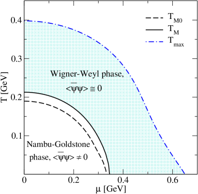
Figure 4: The shaded area shows the region of the phase diagram of strongly interacting quark matter where our computations are applicable. The area is bound by the Mott temperature $T_{\rm M}$ in the case of broken chiral symmetry or $T_{\rm M0}\equiv T_{c}$ in the case where chiral symmetry is intact and by the maximal temperature $T_{\rm max}$ above which no meson modes are found.

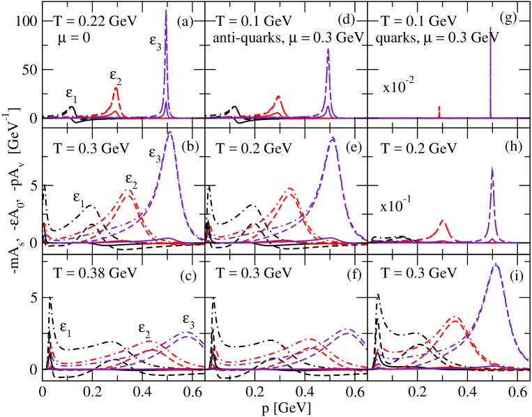
Figure 5: The Lorentz components of the quark and antiquark spectral functions $-mA_{s}$ (solid line), $-\varepsilon A_{0}$ (dash-dotted line) and $-pA_{v}$ (dashed line) as functions of momentum for fixed values of energy. The panels (a)–(c) correspond to $\mu=0$, (d)–(f) – to antiquarks with $\mu=0.3$ GeV, and (g)–(i) – to quarks with $\mu=0.3$ GeV. The spectral functions are evaluated at three energies $\varepsilon_{1}=0.1$, $\varepsilon_{2}=0.3$, and $\varepsilon_{3}=0.5$ GeV.

The quark self-energy corresponding to the meson decays into two quarks and the inverse processes within the regime of interest is given in Matsubara space by LKW15 ; 2017arXiv170204291H

$$\Sigma^{M}(\bm{p},\omega_{n}) =$$

$$=T\sum_{m}\int\frac{d{\bm{q}}}{(2\pi)^{3}}\left[\Gamma_{M}S(\bm{q},\omega_{m})\Gamma_{M}D_{M}(\bm{p}-\bm{q},\omega_{n}-\omega_{m})\right],$$

where $S(\bm{q},\omega_{m})$ is the quark propagator with constituent quark mass, the index $M=\pi,\sigma$ stands for the $\pi$ and $\sigma$ mesons and the vertices are given by $\Gamma_{\sigma}=1$ and $\Gamma_{\pi}=i\gamma_{5}\bm{\tau}$. The Lorentz decomposition of the Matsubara self-energy, which is analogous to (11), is given by

$$\Sigma^{M}(\bm{p},\omega_{n})=P_{M}m\Sigma^{M}_{s}+i\omega_{n}\gamma_{0}\Sigma^{M}_{0}-\bm{p}\cdot\bm{\gamma}\Sigma^{M}_{v},$$ (30)

with $P_{\sigma}=1$, $P_{\pi}=-1$. The computation of the components of this decomposition gives LKW15 ; 2017arXiv170204291H

$$\Sigma^{M}_{s,v} = g^{2}_{M}\int\frac{d\bm{q}}{(2\pi)^{3}}\frac{\mathscr{Q}_{s,v}}{4E_{q}E_{M}}$$ (31)

$$\times \left[\frac{i\omega_{n}\mathscr{C}_{3}-2E_{+}\mathscr{C}_{1}}{E_{+}^{2}+\omega_{n}^{2}}-\frac{i\omega_{n}\mathscr{C}_{3}+2E_{-}\mathscr{C}_{2}}{E_{-}^{2}+\omega_{n}^{2}}\right],$$

$$\Sigma^{M}_{0} = g^{2}_{M}\int\frac{d\bm{q}}{(2\pi)^{3}}\frac{\mathscr{Q}_{0}}{4E_{q}E_{M}}$$ (32)

$$\times \left[\frac{2i\omega_{n}\mathscr{C}_{1}-E_{+}\mathscr{C}_{3}}{E_{+}^{2}+\omega_{n}^{2}}+\frac{2i\omega_{n}\mathscr{C}_{2}+E_{-}\mathscr{C}_{3}}{E_{-}^{2}+\omega_{n}^{2}}\right],$$

where $g_{M}$ is the quark-meson coupling constant and we defined shorthand notations

$$\mathscr{C}_{1}=1+n_{B}(E_{M})-\frac{1}{2}[n^{+}(E_{q})+n^{-}(E_{q})],$$

$$\mathscr{C}_{2}=n_{B}(E_{M})+\frac{1}{2}[n^{+}(E_{q})+n^{-}(E_{q})],$$ (33)

$$\mathscr{C}_{3}=n^{+}(E_{q})-n^{-}(E_{q}),$$

and

$$\mathscr{Q}_{s}=1,\quad\mathscr{Q}_{v}=\frac{\bm{q}\cdot\bm{p}}{p^{2}},\quad\mathscr{Q}_{0}=-\frac{E_{q}}{i\omega_{n}},$$ (34)

with $E_{\pm}=E_{q}\pm E_{q+p}$, $E_{M}=E+E_{p}$, and $E_{p}=\sqrt{p^{2}+m^{2}}$. The distribution functions of quarks and antiquarks are defined as $n^{\pm}(E)=[e^{\beta(E\mp\mu)}+1]^{-1}$, and $n_{B}(E)=(e^{\beta E}-1)^{-1}$ is the Bose distribution function for mesons at zero chemical potential. The retarded self-energy is now obtained by analytical continuation $i\omega_{n}\to p_{0}+i\varepsilon$ and has the same Lorentz structure as its Matsubara counterpart. For the imaginary part of the on-shell quark and antiquark self-energies ($\varrho\equiv{\rm Im}\Sigma$) one finds LKW15 ; 2017arXiv170204291H

$$\varrho_{j}^{M}(p)\Big{|}_{p_{0}=E_{p}}\!\!\! = \frac{g^{2}_{M}}{16\pi p}\int_{E_{\rm min}}^{E_{\rm max}}\!\!\!dE$$ (35)

$$\hskip 28.45274pt\times\mathscr{T}_{j}[n_{B}(E_{M})+n^{-}(E)],\quad$$

$$\varrho^{M}_{j}(p)\Big{|}_{p_{0}=-E_{p}}\!\!\!\! = -\frac{g^{2}_{M}}{16\pi p}\int_{E_{\rm min}}^{E_{\rm max}}\!\!\!\!dE$$ (36)

$$\hskip 28.45274pt\times\mathscr{T}_{j}[n_{B}(E_{M})+n^{+}(E)],\quad$$

where $j=s,0,v,$ $E_{M}=E+E_{p}$, and

$$\mathscr{T}_{s}=1,\quad\mathscr{T}_{v}=\frac{m_{M}^{2}-2m^{2}-2EE_{p}}{2p^{2}},\quad\mathscr{T}_{0}=-\frac{E}{E_{p}}.$$ (37)

The integration limits are defined as

$$E_{{\rm min},{\rm max}} = \frac{1}{2m^{2}}\left[(m_{M}^{2}-2m^{2})p_{0}\right.$$ (38)

$$\hskip 28.45274pt\left.\pm pm_{M}\sqrt{m_{M}^{2}-4m^{2}}\right],$$

and in the chiral limit $m=0$

$$E_{\rm min}=\frac{m_{M}^{2}}{4p},\quad E_{\rm max}\to\infty.$$ (39)

We stress here that Eqs. (35)–(39) are applicable only above the Mott (critical) temperature, where the condition $m_{M}\geq 2m$ is fulfilled. Finally, the full quark-antiquark self-energy in on-shell approximation is written as

$$\varrho_{j}(p_{0},p)=\theta(p_{0})\varrho^{+}_{j}(p)+\theta(-p_{0})\varrho^{-}_{j}(p),$$ (40)

with $\varrho^{\pm}_{j}(p)=\varrho_{j}(p_{0}=\pm E_{p},p)$. From Eqs. (35) and (36) it follows that $\varrho^{+}$ and $\varrho^{-}$ obey the relation $\varrho^{-}_{j}(\mu,p)=-\varrho^{+}_{j}(-\mu,p)$, and, consequently,

$$\varrho_{j}(\mu,-p_{0},p) = -\varrho_{j}(-\mu,p_{0},p).$$ (41)

The contribution of the mesons to the net quark/antiquark self-energy is summed as follows

$$\Sigma_{s}=\Sigma^{\sigma}_{s}-3\Sigma^{\pi}_{s},\quad\Sigma_{0/v}=-\Sigma^{\sigma}_{0/v}-3\Sigma^{\pi}_{0/v}.$$ (42)

In the final step the spectral functions of quarks and antiquarks are constructed according to the relations (13)–(15), where we neglect the real parts which are higher order in the power counting scheme. The numerical results for the components of the spectral function are shown in Fig. 5 and will be used below in the computations of the bulk viscosity.

The key features of spectral functions which are shown for three values of the quark (off-shell) energy ($\varepsilon_{1}=0.1$, $\varepsilon_{2}=0.3$ and $\varepsilon_{3}=0.5$ GeV) are as follows: (a) the spectral functions display a peak at the values of momenta $p\simeq\varepsilon$, which can be anticipated from Eqs. (13)–(15) and is a consequence of the fact that the denominator $d$ attains its minimum roughly at $p\simeq p_{0}$ ($p_{0}\equiv\varepsilon$); (b) the heights of the peaks universally increase with the (off-shell) energies of the quarks; (c) with increasing temperature the dispersive effects become more pronounced, consequently the quasiparticle peaks become broader and the Lorentzian shape of the spectral functions develops in a more complex structure; (d) the main contribution to the spectral function comes from the temporal and vector components, which contribute comparable amounts, whereas the scalar component is small; and (e) the quasiparticle peaks are sharper for quarks rather than for antiquarks for the same values of temperature and chemical potential. Note also that while the Lorentz components of the spectral function may change the sign, the width of the quasiparticles, which is a combination of these, remains positive, which guarantees the overall stability of the system LangDiss .

IV Numerical results for bulk viscosity

We start our analysis with an examination of the influence of various factors entering the expressions for bulk viscosities $\zeta_{0}$, $\zeta_{1}$ and $\zeta_{2}$. Readers interested only in the results on the bulk viscosity can skip to the following subsection.

IV.1 Preliminaries

The behavior of the two-dimensional integrals determining $\zeta_{0}$, $I_{1}$ and $I_{2}$ through Eqs. (17), (24) and (25) is as follows. For a given value of $\varepsilon$ the inner integrands are peaked at $p\simeq|\varepsilon|$, as implied by the shape of the spectral functions. The heights of the peaks rapidly increase with the value of $|\varepsilon|$. As a consequence, the (inner) momentum integrals are increasing functions of $|\varepsilon|$ for $|\varepsilon|\leq\Lambda$. For energies larger than $\Lambda$ the peaks are outside of the momentum-integration range (because of the momentum cutoff $p\leq\Lambda$), and the momentum integral rapidly decreases with $|\varepsilon|$. It vanishes asymptotically in the limit $\varepsilon\to\pm\infty$ for $I_{1}$ and $I_{2}$, but tends to a constant value for $\zeta_{0}$. This asymptotic behavior is easily seen from Eq. (17). Its inner integrand can be roughly estimated as $\propto p^{2}\Big{[}2(\varepsilon^{2}A_{0}-p^{2}A_{v})^{2}-(\varepsilon^{2}-p^{2})(\varepsilon^{2}A_{0}^{2}-p^{2}A_{v}^{2})\Big{]}=p^{2}\Big{[}(\varepsilon^{2}A_{0}-p^{2}A_{v})^{2}+\varepsilon^{2}p^{2}(A_{0}-A_{v})^{2}\Big{]}$, where we approximated $\gamma\simeq 1/3$ and $\delta\simeq 0$ (see Appendix B) and neglected the scalar component of the spectral function, which is small compared to the vector and temporal components. If $|\varepsilon|\gg p$, we can approximate Eqs. (14) and (15) as $n_{1}=\varepsilon^{2}(1-\varrho_{0}^{2})$, $n_{2}=\varepsilon^{2}\varrho_{0}$. The dominant term in the integrand in this case is $\propto p^{2}\varepsilon^{4}A_{0}^{2}=p^{2}\varepsilon^{4}(\varrho_{0}n_{1}-2n_{2})^{2}/(n_{1}^{2}+4n_{2}^{2})^{2}=p^{2}\varrho_{0}^{2}/(1+\varrho_{0}^{2})^{2}$, which does not depend on $\varepsilon$ in the on-shell approximation to the self-energy. As a result, the momentum integral tends to a constant value for $|\varepsilon|\geq\Lambda$. The outer integrals of Eqs. (17), (24) and (25) contain the Fermi factor $\partial n(\varepsilon)/\partial\varepsilon$ which at low temperatures is strongly peaked at the energy $\varepsilon=\mu$. At high temperatures it transforms into a bell-shaped broad structure which samples energies away from $\mu$. We have verified numerically that it is sufficient to integrate up to the energy $|\varepsilon|\leq 2$ GeV. Next we note that the outer integral samples the contribution of antiquarks from the range $(-\infty,0)$ and that of quarks from the range $(0,+\infty)$, and we are in a position to examine these two contributions separately. We find that when $\mu=0$, the integrands of Eqs. (17), (24), and (25) are even functions of $\varepsilon$, i.e., the quark and antiquark contributions are the same. At nonzero chemical potentials the quark-antiquark symmetry is broken and the contributions from quarks and antiquarks differ. While the contributions of quarks and antiquarks to the (inner) momentum integrands are comparable at nonzero $\mu$, the factor $\partial n/\partial\varepsilon$ in the outer energy integration makes the quark contribution dominant.

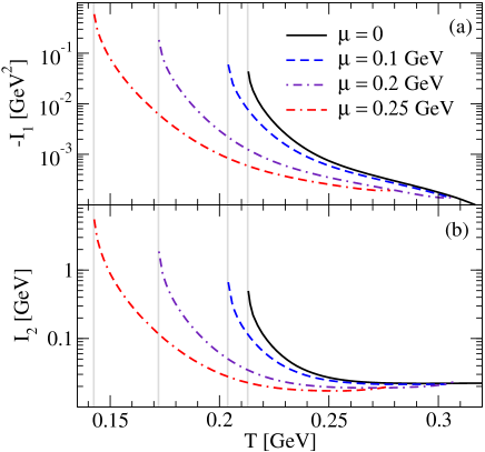
Figure 6: Dependence of the integrals $I_{1}$ and $I_{2}$ on the temperature for several values of the chemical potential. The vertical lines show the Mott temperature at the given value of $\mu$.

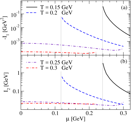
Figure 7: Dependence of the integrals $I_{1}$ and $I_{2}$ on the chemical potential for several values of the temperature. The vertical lines show the values of the chemical potential where the temperature approaches the Mott temperature.

The dependence of the integrals $I_{1}$ and $I_{2}$ on temperature and chemical potential is shown in Figs. 6 and 7. Both are rapidly decreasing functions of temperature (at fixed chemical potential) or chemical potential (at fixed temperature) in the regime close to the Mott line. The observed decrease is the result of broadening of the spectral functions with the temperature, which physically corresponds to stronger dispersive effects and, therefore, smaller values of transport coefficients. Note that in the vicinity of the Mott temperature these quantities become very large because the widths of the spectral functions originating from the imaginary parts of the self-energies vanish for pions and are very small for $\sigma$-mesons. This is partly due to the on-shell approximation to the self-energies. Including off-shell contribution to the self-energies improves the asymptotics close to $T_{M}$, however it is unimportant at temperatures already slightly above the Mott temperature, where the transport coefficients are described by on-shell kinematics quite well LKW15 . In the whole temperature-density range considered $I_{1}$ is always negative, while $I_{2}$ is always positive. $-I_{1}$ is always a decreasing function of the temperature, whereas $I_{2}$ tends to a constant value at high temperatures for small chemical potentials, but shows a slight minimum at higher chemical potentials.

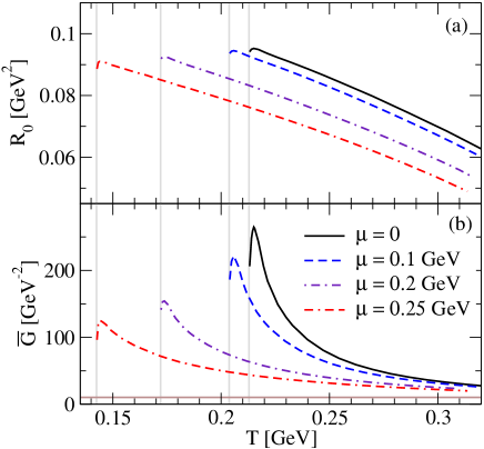
Figure 8: Integral $R_{0}$ (a) and the renormalized coupling $\bar{G}$ (b) as functions of the temperature for various values of the chemical potential. The value of the bare coupling constant $G$ is shown by solid horizontal line.

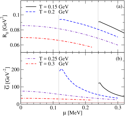
Figure 9: Integral $R_{0}$ (a) and the renormalized coupling $\bar{G}$ (b) as functions of the chemical potential for various values of the temperature. The value of the bare coupling constant $G$ is shown by solid horizontal line.

Next we turn to the discussion of three-dimensional integrals $R_{0}$ and $\bar{R}$, given by Eqs. (23) and (26). A new feature that appears in these expression is the convolution of two spectral functions. As a result, the integrands of $R_{0}$ and $X$ have sharp peaks at $p\simeq|\varepsilon|$ if $|\varepsilon|\simeq|\varepsilon^{\prime}|$, and they transform into broad structures with two smaller maxima located at $p\simeq|\varepsilon|$ and $p\simeq|\varepsilon^{\prime}|$ when $|\varepsilon|\neq|\varepsilon^{\prime}|$. Therefore, the main contribution to the integrals arises from the domain where $p\simeq|\varepsilon|\simeq|\varepsilon^{\prime}|$. Because the integration range covers both positive and negative values of $\varepsilon$ there are two posibilities $\varepsilon^{\prime}=\pm\varepsilon$ for maximum to arise. In the case of $R_{0}$ integral only the minus sign is realized. Indeed, because the temporal and vector components of the spectral function have the same order of magnitude, the inner integrand of $R_{0}$ can be roughly estimated as $aa^{\prime}+bb^{\prime}-cc^{\prime}\simeq\varepsilon\varepsilon^{\prime}A_{0}A_{0}^{\prime}-p^{2}A_{v}A_{v}^{\prime}\simeq(\varepsilon\varepsilon^{\prime}-p^{2})A_{0}A_{0}^{\prime}$, see Eqs. (23). Therefore, the peaks around $p\simeq\varepsilon\simeq\varepsilon^{\prime}$ originating from temporal and vector components almost cancel each other, and the momentum integral is mainly concentrated around $\varepsilon^{\prime}\simeq-\varepsilon$. The integral $\bar{R}$ contains additional terms which support also a peak at $\varepsilon^{\prime}\simeq\varepsilon$ and, consequently, the momentum integrand obtains contributions at two locations. In both cases of $R_{0}$ and $\bar{R}$, the height of the peaks rapidly increases with the increase of $|\varepsilon|$ as long as $|\varepsilon|\leq\Lambda$ and becomes negligible for higher values of $|\varepsilon|$. The integration over $\varepsilon^{\prime}$ contains also the factor $[n(\varepsilon)-n(\varepsilon^{\prime})]/(\varepsilon-\varepsilon^{\prime})$ which at low temperatures is strongly peaked at the energies $\varepsilon=\varepsilon^{\prime}=\mu$. At high temperatures it transforms into a bell-shaped broad structure (without change of the location of the maximum) and samples energies far away from $\mu$. It decreases faster at high energies in the case when $\varepsilon-\mu$ and $\varepsilon^{\prime}-\mu$ have the same sign. The integrand of $\bar{R}$ contains an additional combination of Fermi functions $[\varepsilon n(\varepsilon)-\varepsilon^{\prime}n(\varepsilon^{\prime})]/(\varepsilon-\varepsilon^{\prime})-1/2$, which tends to the finite limits $-1/2$ and $1/2$, when $\varepsilon,\varepsilon^{\prime}\to+\infty$ and $\varepsilon,\varepsilon^{\prime}\to-\infty$, respectively.

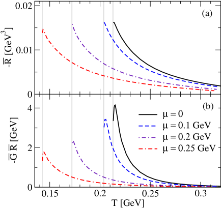
Figure 10: Integral $\bar{R}$ (a) and the product $\bar{G}\bar{R}$ (b) as functions of the temperature for various values of the chemical potential.

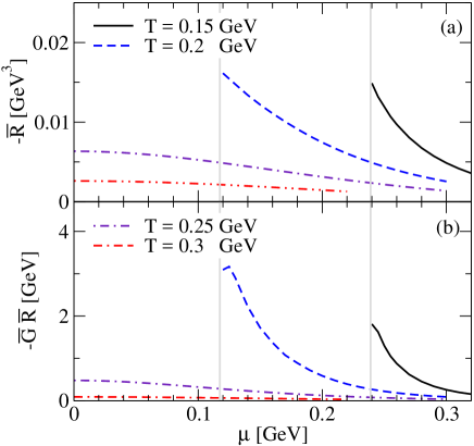
Figure 11: Integral $\bar{R}$ (a) and the product $\bar{G}\bar{R}$ (b) as functions of the chemical potential for various values of the temperature.

The outer integrands of $R_{0}$ and $\bar{R}$ are rapidly increasing functions of $|\varepsilon|$ for $|\varepsilon|\leq\Lambda$ and they sharply drop at higher values of $|\varepsilon|$, as it was the case for the two-dimensional integrals $I_{1}$ and $I_{2}$. Our analysis shows that the momentum integrals in Eqs. (23) and (26) are invariant under the simultaneous transformations $\varepsilon\to-\varepsilon$, $\varepsilon^{\prime}\to-\varepsilon^{\prime}$, $\mu\to-\mu$, as expected. Due to this property all integrals are even functions of the chemical potential.

Figures 8 and 9 illustrate the temperature and chemical potential dependence of the integral $R_{0}$ and the renormalized coupling (22). The same dependence for the integral $\bar{R}$ and the product $\bar{G}\bar{R}$ is shown in Figs. 10 and 11. The latter combination enters the formulas of $\zeta_{1,2}$ components of the bulk viscosity, see Eq. (21). It is remarkable that $R_{0}$ and $\bar{R}$ remain finite at the Mott temperature in contrast to the integrals $I_{1}$ and $I_{2}$. The reason for this behavior can be understood if we recall that at the Mott temperature the imaginary parts of the self-energies essentially vanish, therefore the spectral functions transform into $\delta$-functions: $A_{j}(p,\varepsilon)\propto\delta(p^{2}+m^{2}-\varepsilon^{2})$, where $j$ index labels the Lorentz component. Therefore, the integrands of the expressions (23) and (26) will contain a product of two $\delta$-functions at different arguments. When integrated over the variables $\varepsilon$ and $\varepsilon^{\prime}$, the integral will consequently have a finite value. (This was not the case for two-dimensional intergals, where a single energy-integration led to two $\delta$-functions at the same argument and, therefore, to a divergent integral.) Apart the different asymptotics for $T\to T_{M}$, the generic temperature-density dependence of the three-dimensional intergrals $R_{0}$ and $\bar{R}$ does not differ significantly from that of two-dimensional integrals discussed above. Close to the Mott line we find $R_{0}\simeq 0.1$ GeV² and, therefore, $\bar{G}\gg G\simeq 10$ GeV^-2. At high temperatures and chemical potentials $R_{0}$ decreases, and $\bar{G}$ tends to its “bare” value. Thus, we conclude that the renormalization of the coupling constant by multiloop contributions and its effect on the bulk viscosity should be important in the low-temperature regime close to the Mott transition line. We also note that $\bar{R}$ is alway negative, which in combination with $I_{1}<0$ and $I_{2}>0$ guarantees the positivity of both components $\zeta_{1}$ and $\zeta_{2}$ in the entire temperature-density range.

IV.2 Bulk viscosities

With the analysis above we are in a position to study the behavior of the components of the bulk viscosity $\zeta_{0}$, $\zeta_{1}$, $\zeta_{2}$ and their sum $\zeta$. Figures 12 and 13 show these quantities as functions of temperature and chemical potential, respectively. Because, as we have seen, the functions $|I_{1}|$, $I_{2}$, as well as $R_{0}$, $\bar{G}$ and $|\bar{R}|$ display a maximum at (or close to) the Mott line and decay with increasing temperature or chemical potential, the multiloop contributions to the bulk viscosity $\zeta_{1}$ and $\zeta_{2}$ are expected to show analogous behavior. The one-loop result $\zeta_{0}$ is maximal at the Mott line as well, decreases with increasing $T$ or $\mu$, passes a minimum and increases according to a power law. At high temperatures the temperature scaling is $\zeta_{0}\propto T^{3}$. This functional behavior arises from the fact that $\zeta_{0}$ depends essentially on the difference of the temporal and vector components of the spectral function, see Eqs. (17)–(19), and its asymptotic increase for large $\mu$ or $T$ has been verified to be the result of the increase of difference between those components with increasing $T$ or $\mu$, see Fig. 5. This is also the reason why the bulk viscosity evaluated in the one-loop approximation is negligible compared to the shear viscosity, since the latter depends on the average amplitude of the spectral functions LKW15 ; 2017arXiv170204291H .

The contribution from the multiloop processes dominates the one-loop result close to the corresponding Mott line, i.e., at sufficiently low temperatures or chemical potentials, see Figs. 12 and 13. In this regime all three components $\zeta_{0}$, $\zeta_{1}$, $\zeta_{2}$ and, therefore, also the net bulk viscosity $\zeta$ drop rapidly with increasing temperature or chemical potential. The functional behavior of three components of the bulk viscosity around the Mott line is described by the universal formula

$$\zeta_{i}\sim\exp\left(\frac{a_{i}}{T/T_{M}-b_{i}}\right),\quad i=0,1,2,$$ (43)

where $a_{i}$ and $b_{i}\lesssim 1$ depend only on the chemical potential. In this regime the following inequalities hold $\zeta\simeq\zeta_{2}\gg\zeta_{1}\gg\zeta_{0}$, and we see from Figs. 12 and 13 that the one-loop result $\zeta_{0}$ underestimates the net bulk viscosity by three orders of magnitude.

The situation reverses for high $T$ and $\mu$, where the multiloop contributions $\zeta_{1}$ and $\zeta_{2}$ decrease rapidly and one finds $\zeta\simeq\zeta_{0}\gg\zeta_{2}\gg\zeta_{1}$. As a consequence, the net bulk viscosity has a mild minimum as a function of temperature. In the high-temperature regime it increases as $\zeta\propto T^{3}$, but is almost independent on the chemical potential.

Thus, we conclude that in the high-$T$ or high-$\mu$ limits the single-loop approximation correctly represents the bulk viscosity, i.e., the single-loop provides indeed the leading-order contribution. This is clearly not the case in the low-$T$ or low-$\mu$ limits, close to the Mott line, where $\zeta_{0}$ fails to describe correctly the bulk viscosity, which is dominated by the multiloop contributions from $\zeta_{2}$.

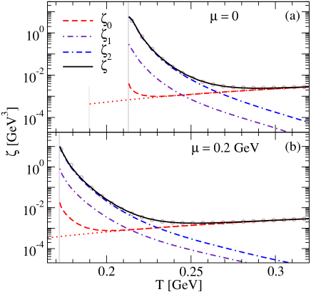
Figure 12: The three components of the bulk viscosity and their sum as functions of the temperature for two values of the chemical potential. The dotted lines correspond to the chiral limit $m_{0}=0$. The results of the fit formula (44) are shown by circles.

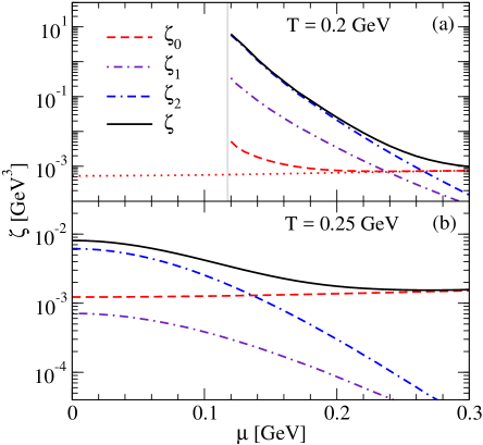
Figure 13: The three components of the bulk viscosity and their sum as functions of the chemical potential for two values of the temperature. The dotted lines correspond to the chiral limit $m_{0}=0$.

IV.3 Chiral limit

It is interesting to explore the case when the chiral symmetry is intact ($m_{0}=0$). In this case quarks become massless above the critical (Mott) temperature $T_{c}$, which implies vanishing multiloop contributions, as already mentioned in Sec. II. Consequently, the bulk viscosity is determined by the single-loop result (17) with $m=m_{0}=0$. As seen from Figs. 12 and 13, $\zeta_{0}$ behaves quite differently in the chiral limit from the case of $m_{0}\neq 0$ close to the Mott temperature. It is smooth at the critical temperature and increases with the temperature by a cubic law in the entire parameter range. This behavior can be understood as follows. At $T\to T_{c}$ we have $m=0$, $m_{M}\to 0$, therefore from Eqs. (35)–(39) we find $\varrho_{0}\simeq\varrho_{v}\to 0$ for high momenta which contribute mostly to $\zeta_{0}$. Therefore, from Eqs. (13)–(15) we estimate $n_{1}\simeq p_{0}^{2}-p^{2}$, $n_{2}\simeq(p_{0}^{2}-p^{2})\varrho_{0}\to 0$ and $A_{0,v}(p_{0},p)\simeq-n_{2}/(n_{1}^{2}+4n_{2}^{2})\sim\delta(p_{0}^{2}-p^{2})$. Now substituting $\gamma=1/3$, $\delta=0$ in Eqs. (17)–(19) (see Appendix B) we find that the integrand of $\zeta_{0}$ is proportional to $2(\varepsilon^{2}A_{0}-p^{2}A_{v})^{2}-(\varepsilon^{2}-p^{2})(\varepsilon^{2}A_{0}^{2}-p^{2}A_{v}^{2})\sim(\varepsilon^{2}-p^{2})^{2}\delta(\varepsilon^{2}-p^{2})^{2}\to 0$, which implies that the integral remains regular in the limit $T\to T_{c}$. In the high-$T$ regime the results for $\zeta_{0}$ coincide with those of the case of explicit chiral symmetry breaking.

We note that according to the discussion above $\zeta_{0}$ component will vanish in any theory with weakly-interacting massless particles. The weakness of the interaction implies small spectral widths and, therefore, nearly on-mass-shell particles with $p=\varepsilon$. As a consequence, the integrand in Eq. (17) vanishes, as expected.

IV.4 Comparison to shear viscosity

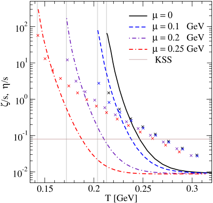
Figure 14: The ratio $\zeta/s$ as function of the temperature for several values of the chemical potential. The corresponding $\eta/s$ ratios are shown for comparison by crosses. The solid horizontal line shows the KSS bound 2005PhRvL..94k1601K .

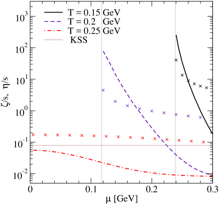
Figure 15: The ratio $\zeta/s$ as function of the chemical potential for several values of the temperature. The corresponding ratios $\eta/s$ are shown by crosses. The solid horizontal line shows the KSS bound 2005PhRvL..94k1601K .

In Figs. 14 and 15 we show the dependence of the ratio $\zeta/s$ on temperature and chemical potential, where $s$ is the entropy density, see Appendix B. For comparison we show also the ratio $\eta/s$ as computed in Refs. LKW15 ; 2017arXiv170204291H and the AdS/CFT lower bound $1/4\pi$ on that ratio 2005PhRvL..94k1601K . As a general trend, the ratio $\zeta/s$ increases rapidly close to the Mott transition line with decreasing temperature or chemical potential and attains its maximum on this line. It becomes weakly dependent on these quantities as one moves away from this regime to high-$\mu$ and high-$T$ limit. The $\eta/s$ displays similar behavior, but the increase in the vicinity of the Mott line is not as steep as for $\zeta/s$. Numerically we find in this regime $\zeta\geq\eta$ with $\zeta/\eta\simeq 5\div 20$ on the Mott line. Thus, we conclude that close to the Mott transition line the bulk viscosity dominates the shear viscosity by large factors and this dominance arises from the multiloop processes. We stress that had we kept only the one-loop contribution to the bulk viscosity, it would have been negligible compared to the shear viscosity. As the temperature or the chemical potential increases away from the Mott line, $\zeta$ decreases faster than $\eta$ and eventually one reaches the point where $\zeta=\eta$, beyond which shear viscosity dominates. This crossover point appears earlier than the point where $\zeta_{0}\simeq\zeta_{2}$ beyond which $\zeta_{0}$ dominates the bulk viscosity, see the next subsection. Consequently, we conclude that if only $\zeta_{0}$ contribution is kept, then shear viscosity is the dominant source of dissipation in the entire temperature-density regime.

In closing we note that in the $T$-$\mu$ region where $\eta$ drops below the AdS/CFT value $1/4\pi$, the quark-meson fluctuations considered in this work may not be the dominant processes controlling the viscous dissipation. Pure gauge fluctuations as well as quark-quark scattering processes may contribute substantially in this range of parameters thereby raising the value of $\eta/s$ above the conjectured bound.

IV.5 Fits to the bulk viscosity

The observed nearly universal low-$T$ behavior (43) of $\zeta_{2}$ component with the scaled temperature $T/T_{\rm M}$ for fixed values of the chemical potential and the high-$T$ asymptotics of $\zeta_{0}$ suggest fitting the net bulk viscosity in the whole temperature range by the formula

$$\zeta_{\rm fit}(T,\mu)=a(y)\exp\left[\frac{c(y)}{T/T_{M}(y)-b(y)}\right]+d(y)T^{3},$$ (44)

with $y=\mu/\mu_{0}$, where $\mu_{0}=0.345$ GeV corresponds to the point where $T_{\rm M}=0$ and the chemical potential attains its maximum on the Mott line. The coefficients $a,b,c,d$ are given by

$$a(y) = (2.57-5.65y^{2})\times 10^{-6}\hskip 2.84544pt[{\rm GeV}^{3}],$$ (45)

$$b(y) = 0.806-0.055y^{2}-0.617y^{4},$$ (46)

$$c(y) = 2.89+0.96y^{2}+12.73y^{4},$$ (47)

$$d(y) = 0.082+0.02y^{2}.$$ (48)

The fit formula (44) is valid for chemical potentials $\mu\leq 0.2$ GeV, where its relative error is $\leq 10\%$. A comparison of the fit with the numerical result is given in Fig. 12.

In the chiral limit the first term in Eq. (44) vanishes, and we are left with pure power-low increase in the whole temperature-density range

$$\zeta_{\rm ch}(T,\mu)=T^{3}(0.082+0.168\mu^{2}),$$ (49)

where $T$ and $\mu$ are in GeV units.

We fit also the Mott temperature displayed in Fig. 4 with the formula

$$T_{\rm M}^{\rm fit}(\mu)=T_{0}\left\{\begin{array}[]{ll}1-\sqrt{\gamma y}e^{-\pi/(\gamma y)}&0\leq y\leq 0.5,\\ \sqrt{1.55(1-y)+0.04(1-y)^{2}}&0.5<y\leq 1,\end{array}\right.$$ (52)

with $T_{0}=T_{\rm M}(\mu=0)=0.213$ GeV, and $\gamma=2.7$. The formula (52) has relative accuracy $\leq 3\%$ for chemical potentials $\mu\leq 0.32$ GeV.

Now we define several characteristic temperatures: $T_{\rm min}^{0}$ and $T_{\rm min}$, corresponding to the minimums of $\zeta_{0}$ and $\zeta$, respectively; $T_{02}$ - the temperature of intersection of $\zeta_{0}$ and $\zeta_{2}$ components; and $T_{\zeta=\eta}$ - the temperature of intersection of $\zeta$ and $\eta$. These temperatures vary with the chemical potential, or, equivalently, with the corresponding value of the Mott temperature. Interestingly, all these characteristic temperatures turn out to be linear functions of the Mott temperature with $1\%$ accuracy and can be fitted as

$$T^{*}(\mu)=\alpha T_{\rm M}(\mu)+\Delta,$$ (54)

where $T^{*}=\{T_{\rm min}^{0},T_{\rm min},T_{02},T_{\zeta=\eta}\}$, and the coefficients $\alpha$ and $\Delta$ do not depend on the chemical potential. Their numerical values are listed in Table 1.

$T^{*}$	$\quad\alpha\quad$	$\quad\Delta$ [GeV]
$T_{\rm min}^{0}$	0.65	0.09
$T_{\rm min}$	0.86	0.106
$T_{02}$	0.84	0.087
$T_{\eta=\zeta}$	1.13	-6$\cdot 10^{-3}$

Table 1: The values of the fit parameters in Eq. (54).

V Conclusions

On the formal side, this work provides a derivation of the bulk viscosity for relativistic quantum fields in terms of the Lorentz components of their spectral function within the Kubo-Zubarev formalism 1957JPSJ…12..570K ; zubarev1997statistical . It complements similar expressions for the shear viscosity LKW15 and the electrical and thermal conductivities 2017arXiv170204291H derived earlier.

Practical computations of the bulk viscosity via two-point correlation function have been carried out within the two-flavor NJL model. The relevant diagrams were selected by using the $1/N_{c}$ expansion, where $N_{c}$ is the number of colors.

One of our key results is the observation that the single-loop contributions, which are dominant for shear viscosity and conductivities, are insufficient for the evaluation of the bulk viscosity. We demonstrated that close to the Mott temperature multiloop contributions, which require resummations of infinite geometrical series of loops, dominate the one-loop contribution. We concentrated on the regime where the dispersive effects arise from quark-meson scattering above the Mott temperature for decay of mesons (pions and sigmas) into quarks. In this regime the bulk viscosity is a decreasing function of temperature at fixed chemical potential, but after passing a minimum it increases again. The decreasing behavior is dominated by multiloop contribution, whereas the high-$T$ increasing segment is dominated by the one-loop contribution.

Another key result of this study is the observation that the bulk viscosity dominates the shear viscosity of quark matter in the vicinity of the Mott temperature by factors of $5\div 20$ depending on the chemical potential. With increasing temperature the bulk viscosity decreases faster than the shear viscosity and above a certain temperature we find $\eta\geq\zeta$. The range of validity of our comparison is limited by the temperature at which the ratio $\eta/s$ undershoots the KSS bound $1/4\pi$ and obviously the dispersive effects due to mesonic decays into quarks are insufficient to account for the shear viscosity of quark matter. Nevertheless, the observation of large bulk viscosity in the parameter domain of this study may have interesting and important implications for the hydrodynamical description of heavy-ion collisions at the RHIC and LHC.

Looking ahead, we anticipate that the formalism described here can be straightforwardly extended to include heavier flavor quarks, most important being the strange quark. The NJL-model Lagrangian can be extended to include vector interactions and/or Polyakov loop contributions. As the gluonic degrees of freedom are integrated out in the NJL-type models from the outset, the pure gauge contributions can be accounted only if one starts with an effective model that captures the gauge sector of QCD.

Appendix A Calculation of the bulk viscosity

Substituting Eq. (6) into Eq. (5) and taking into account the isotropy of the medium ($[T_{11},T_{33}]=[T_{11},T_{22}]$ etc.) and the symmetry property of correlation function in its arguments 2011AnPhy.326.3075H we obtain

$$\Pi^{R}_{\zeta}(\omega) = -i\int_{0}^{\infty}dte^{i\omega t}\int d\bm{r}\langle\frac{1}{3}[T_{11},T_{11}]+\frac{2}{3}[T_{11},T_{22}]-2\gamma[T_{11},T_{00}]$$ (55)

$$-2\delta[T_{11},N_{0}]+2\gamma\delta[T_{00},N_{0}]+\gamma^{2}[T_{00},T_{00}]+\delta^{2}[N_{0},N_{0}]\rangle_{0}.$$

Further progress requires substituting the explicit expressions for the components of the energy-momentum tensor (2) and the particle current (3) in this expression. We first switch to the imaginary time formalism by replacement $t\to-i\tau$ and introduce shorthand notation

$$\Pi^{(kl)}[\hat{a},\hat{b}](\omega_{n})=\bigg{(}\frac{G}{2}\bigg{)}^{k+l-2}\int_{0}^{\beta}d\tau\ e^{i\omega_{n}\tau}\int d\bm{r}\langle T_{\tau}\big{(}(\bar{\psi}\hat{a}\psi)^{k}\Big{|}_{(\bm{r},\tau)},(\bar{\psi}\hat{b}\psi)^{l}\Big{|}_{0})\rangle_{0},$$ (56)

where $\hat{a}$ and $\hat{b}$ are either differential operators (contracted with Dirac $\gamma$ matrices) or interaction vertices $\Gamma^{0}_{s/ps}$ appearing in Eqs. (1)–(3). Then the result of the substitution can be written as a sum of three terms

$$\Pi^{M}_{\zeta}(\omega_{n})=\Pi^{M,11}_{\zeta}(\omega_{n})+\Pi^{M,12}_{\zeta}(\omega_{n})+\Pi^{M,22}_{\zeta}(\omega_{n}),$$ (57)

where

$$-\Pi^{M,11}_{\zeta}(\omega_{n}) = \frac{1}{3}\Pi^{(11)}[i\gamma_{1}\partial_{1},i\gamma_{1}\partial_{1}]+\frac{2}{3}\Pi^{(11)}[i\gamma_{1}\partial_{1},i\gamma_{2}\partial_{2}]-2\gamma\Pi^{(11)}[i\gamma_{1}\partial_{1},-\gamma_{0}\partial_{\tau}]$$ (58)

$$- 2\delta\Pi^{(11)}[i\gamma_{1}\partial_{1},\gamma_{0}]+2\gamma\delta\Pi^{(11)}[-\gamma_{0}\partial_{\tau},\gamma_{0}]+\gamma^{2}\Pi^{(11)}[-\gamma_{0}\partial_{\tau},-\gamma_{0}\partial_{\tau}]$$

$$+ \delta^{2}\Pi^{(11)}[\gamma_{0},\gamma_{0}]+2(1+\gamma)\Pi^{(11)}[i\gamma_{1}\partial_{1},i\not{\partial}_{\tau}-m_{0}]-2\gamma(1+\gamma)\Pi^{(11)}[-\gamma_{0}\partial_{\tau},i\not{\partial}_{\tau}-m_{0}]$$

$$- 2\delta(1+\gamma)\Pi^{(11)}[\gamma_{0},i\not{\partial}_{\tau}-m_{0}]+(1+\gamma)^{2}\Pi^{(11)}[i\not{\partial}_{\tau}-m_{0},i\not{\partial}_{\tau}-m_{0}],$$

and

$$-\Pi^{M,12}_{\zeta}(\omega_{n}) = 2(1+\gamma)\sum\limits_{\Gamma=\{1,i\bm{\tau}\gamma_{5}\}}\Pi^{(12)}[i\gamma_{1}\partial_{1},\Gamma]-2\gamma(1+\gamma)\sum\limits_{\Gamma=\{1,i\bm{\tau}\gamma_{5}\}}\Pi^{(12)}[-\gamma_{0}\partial_{\tau},\Gamma]$$ (59)

$$- 2\delta(1+\gamma)\sum\limits_{\Gamma=\{1,i\bm{\tau}\gamma_{5}\}}\Pi^{(12)}[\gamma_{0},\Gamma]+2(1+\gamma)^{2}\sum\limits_{\Gamma=\{1,i\bm{\tau}\gamma_{5}\}}\Pi^{(12)}[i\not{\partial}_{\tau}-m_{0},\Gamma],$$

$$-\Pi^{M,22}_{\zeta}(\omega_{n}) = (1+\gamma)^{2}\sum\limits_{\Gamma,\Gamma^{\prime}=\{1,i\bm{\tau}\gamma_{5}\}}\Pi^{(22)}[\Gamma,\Gamma^{\prime}].$$ (60)

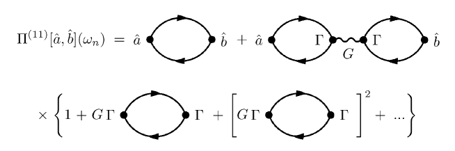
Figure 16: Loop resummation for the correlation function $\Pi^{(11)}[\hat{a},\hat{b}]$ defined in Eq. (56) at leading order in $1/N_{c}$ expansion.

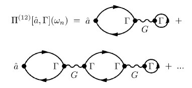
Figure 17: Same as Fig. 16, but for the function $\Pi^{(12)}[\hat{a},\Gamma$].

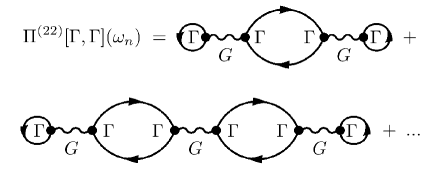
Figure 18: Same as Fig. 16, but for the function $\Pi^{(22)}[\Gamma,\Gamma$].

The three types of correlation functions entering Eqs. (57)–(60) are shown in Figs. 16–18. Next we note that $\Pi^{(12)}[\hat{a},\Gamma](\omega_{n})=\Pi^{(22)}[\Gamma,\Gamma^{\prime}](\omega_{n})=0,$ because both contain bubble diagrams with one vertex $\Gamma$, which permits only $\omega_{n}=0$. Thus, the second and the third terms in Eq. (57) vanish. We also note that the pseudoscalar vertex with $\gamma_{5}$ does not appear in this expression, therefore we are left in all diagrams with the vertex $\Gamma=1$.

The remaining terms in the two-point correlation function can be expressed through the single-loop diagrams given by Eq. (9) of the main text. With this definition and from Fig. 16 we find that

$$\Pi^{(11)}[\hat{a},\hat{b}]=\Pi_{0}[\hat{a},\hat{b}]+\tilde{G}\Pi_{0}[\hat{a},1]\Pi_{0}[1,\hat{b}],$$ (61)

where we introduced a frequency-dependent coupling constant

$$\tilde{G}(\omega_{n})=\frac{G}{1-G\Pi_{0}[1,1](\omega_{n})}.$$ (62)

To perform the Matsubara sums we need to take into account that the operators $\hat{a}$ and $\hat{b}$ may depend on $i\omega_{l}$. (For example, if $\hat{a}=-\gamma_{0}\partial_{\tau}$, in the momentum space we have $\hat{a}=i\gamma_{0}\bar{\omega}_{l}$, $\bar{\omega}_{l}=\omega_{l}+\omega_{n}/2$.) We separate the $i\bar{\omega}_{l}$-dependent parts of these operators by formally factorizing $\hat{a}...\hat{b}...=f(i\bar{\omega}_{l})\hat{a}_{0}...\hat{b_{0}}...$, where $\hat{a}_{0}$ and $\hat{b}_{0}$ are $i\bar{\omega}_{l}$-independent parts of operators $\hat{a}$ and $\hat{b}$. Applying this definition we find

$$S[\hat{a},\hat{b}](\bm{p},i\omega_{n}) \equiv T\sum\limits_{l}{\rm Tr}\bigl{[}\hat{a}G(\bm{p},i\omega_{l}+i\omega_{n})\hat{b}G(\bm{p},i\omega_{l})\bigr{]}$$ (63)

$$=T\sum\limits_{l}f(i\bar{\omega}_{l}){\rm Tr}\bigl{[}\hat{a}_{0}G(\bm{p},i\omega_{l}+i\omega_{n})\hat{b}_{0}G(\bm{p},i\omega_{l})\bigr{]}.$$

After summation over the Matsubara frequencies and subsequent analytical continuation $i\omega_{n}=\omega_{n}+i\delta$ we obtain

$$S[\hat{a},\hat{b}](\bm{p},\omega)=\int_{-\infty}^{\infty}d\varepsilon\int_{-\infty}^{\infty}d\varepsilon^{\prime}{\rm Tr}[\hat{a}_{0}A(\bm{p},\varepsilon^{\prime})\hat{b}_{0}A(\bm{p},\varepsilon)]$$

$$\times\frac{\tilde{n}(\varepsilon)f(\varepsilon+\omega/2)-\tilde{n}(\varepsilon^{\prime})f(\varepsilon^{\prime}-\omega/2)}{\varepsilon-\varepsilon^{\prime}+\omega+i\delta},\hskip 14.22636pt$$ (64)

where we used the spectral representation

$$G(\bm{p},z)=\int_{-\infty}^{\infty}d\varepsilon\frac{A(\bm{p},\varepsilon)}{z-\varepsilon}.$$ (65)

This implies that the single-loop polarization tensor is given by

$$\Pi_{0}[\hat{a},\hat{b}](\omega)=\int\frac{d\bm{p}}{(2\pi)^{3}}\int_{-\infty}^{\infty}d\varepsilon\int_{-\infty}^{\infty}d\varepsilon^{\prime}{\rm Tr}[\hat{a}_{0}A(\bm{p},\varepsilon^{\prime})\hat{b}_{0}$$

$$\times A(\bm{p},\varepsilon)]\frac{\tilde{n}(\varepsilon^{\prime})f(\varepsilon^{\prime}-\omega/2)-\tilde{n}(\varepsilon)f(\varepsilon+\omega/2)}{\varepsilon-\varepsilon^{\prime}+\omega+i\delta}.\hskip 21.33955pt$$ (66)

The real and imaginary parts of the polarization tensor can now be computed by applying the Dirac identity. In particular, we find

$${\rm Im}\Pi_{0}[\hat{a},\hat{b}](\omega)\Big{|}_{\omega=0}=\frac{d}{d\omega}{\rm Re}\Pi_{0}[\hat{a},\hat{b}](\omega)\Big{|}_{\omega=0}=0.$$ (67)

Next we compute from the polarization tensor the relevant structure needed for the bulk viscosity by defining

$$\frac{d}{d\omega}{\rm Im}\Pi^{(11)}[\hat{a},\hat{b}](\omega)\bigg{|}_{\omega=0}\hskip 71.13188pt$$

$$=L_{0}[\hat{a},\hat{b}]+\bar{G}L_{1}[\hat{a},\hat{b}]+\bar{G}^{2}L_{2}[\hat{a},\hat{b}],$$ (68)

where

$$L_{0}[\hat{a},\hat{b}] = \frac{d}{d\omega}{\rm Im}\Pi_{0}[\hat{a},\hat{b}](\omega)\big{|}_{\omega=0},$$ (69)

$$L_{1}[\hat{a},\hat{b}] = R_{0}[\hat{a},1]L_{0}[1,\hat{b}]+R_{0}[1,\hat{b}]L_{0}[\hat{a},1],\quad$$ (70)

$$L_{2}[\hat{a},\hat{b}] = L_{0}[1,1]R_{0}[\hat{a},1]R_{0}[1,\hat{b}],$$ (71)

$$R_{0}[\hat{a},\hat{b}] = {\rm Re}\Pi_{0}[\hat{a},\hat{b}]\big{|}_{\omega=0},$$ (72)

and the effective zero-frequency coupling is given by

$$\bar{G}\equiv{\rm Re}\bar{G}\big{|}_{\omega=0}=\frac{G}{1-GR_{0}[1,1]}.$$ (73)

Now we calculate the relevant pieces of the polarization for specific $\hat{a}$ and $\hat{b}$ operator combinations. The relevant real parts can be written in the generic form

$$R_{0}[\hat{a},\hat{b}] = -\frac{2N_{c}N_{f}}{\pi^{4}}\!\!\int_{0}^{\Lambda}\!\!\!dp\int_{-\infty}^{\infty}\!\!\!d\varepsilon\int_{-\infty}^{\infty}\!\!\!d\varepsilon^{\prime}$$ (74)

$$\frac{\varepsilon^{k}\tilde{n}(\varepsilon)-\varepsilon^{\prime k}\tilde{n}(\varepsilon^{\prime})}{\varepsilon-\varepsilon^{\prime}}{\cal O}_{R}(p,\varepsilon,\varepsilon^{\prime}),\qquad$$

where the factors $N_{c}=3$ and $N_{f}=2$ arise from the trace in the color and flavor spaces, respectively; $\Lambda$ is the 3-momentum cutoff parameter. For each specific value of $\hat{a}$ and $\hat{b}$ operators we have the following functions ${\cal O}_{R}$

$$R_{0}\left[1,1\right]\quad {\cal O}_{R}=p^{2}(m^{2}A_{s}A^{\prime}_{s}+\varepsilon\varepsilon^{\prime}A_{0}A_{0}^{\prime}$$ (75a)

$$\hskip 80.52135pt-p^{2}A_{v}A_{v}^{\prime}),\hskip 28.45274pt$$

$$R_{0}\left[1,i\gamma_{1}\partial_{1}\right]\quad {\cal O}_{R}=\frac{1}{3}mp^{4}(A_{s}^{\prime}A_{v}+A_{s}A_{v}^{\prime}),$$ (75b)

$$R_{0}\left[1,\gamma_{0}\right]\quad {\cal O}_{R}=mp^{2}(\varepsilon A_{s}^{\prime}A_{0}+\varepsilon^{\prime}A_{s}A_{0}^{\prime}),$$ (75c)

$$R_{0}\left[1,-\gamma_{0}\partial_{\tau}\right]\quad {\cal O}_{R}=mp^{2}(\varepsilon A_{s}^{\prime}A_{0}+\varepsilon^{\prime}A_{s}A_{0}^{\prime}),$$ (75d)

and $$k=0 k=1$$ for the first three cases and for the last case.

The generic form of the imaginary parts is given by

$$L_{0}[\hat{a},\hat{b}]=-\frac{2N_{c}N_{f}}{\pi^{3}}\int_{0}^{\Lambda}dp\int_{-\infty}^{\infty}d\varepsilon n^{\prime}(\varepsilon){\cal O}_{I}(p,\varepsilon),\quad$$ (76)

where for each specific value of $\hat{a}$ and $\hat{b}$ operators the following ${\cal O}_{I}$ functions should be substituted

$$L_{0}[1,1] {\cal O}_{I}=p^{2}(m^{2}A_{s}^{2}+\varepsilon^{2}A_{0}^{2}-p^{2}A_{v}^{2}),$$

$$L_{0}[1,\gamma_{0}] {\cal O}_{I}=2mp^{2}\varepsilon A_{s}A_{0},$$ (77b)

$$L_{0}[1,-\gamma_{0}\partial_{\tau}] {\cal O}_{I}=2mp^{2}\varepsilon^{2}A_{s}A_{0},$$ (77c)

$$L_{0}[1,i\gamma_{1}\partial_{1}] {\cal O}_{I}=\frac{2}{3}mp^{4}A_{s}A_{v},$$ (77d)

$$L_{0}[\gamma_{0},\gamma_{0}] {\cal O}_{I}=p^{2}(m^{2}A_{s}^{2}+\varepsilon^{2}A_{0}^{2}+p^{2}A_{v}^{2}),$$

$$L_{0}[-\gamma_{0}\partial_{\tau},-\gamma_{0}\partial_{\tau}] {\cal O}_{I}=p^{2}\varepsilon^{2}(m^{2}A_{s}^{2}+\varepsilon^{2}A_{0}^{2}+p^{2}A_{v}^{2}),$$

$$L_{0}[\gamma_{0},-\gamma_{0}\partial_{\tau}] {\cal O}_{I}=p^{2}\varepsilon(m^{2}A_{s}^{2}+\varepsilon^{2}A_{0}^{2}+p^{2}A_{v}^{2}),$$

$$L_{0}[i\gamma_{1}\partial_{1},\gamma_{0}] {\cal O}_{I}=\frac{2}{3}p^{4}\varepsilon A_{0}A_{v},$$ (77h)

$$L_{0}[i\gamma_{1}\partial_{1},-\gamma_{0}\partial_{\tau}] {\cal O}_{I}=\frac{2}{3}p^{4}\varepsilon^{2}A_{0}A_{v},$$ (77i)

$$L_{0}[i\gamma_{1}\partial_{1},i\gamma_{1}\partial_{1}] {\cal O}_{I}=\frac{p^{4}}{15}(-5m^{2}A_{s}^{2}+5\varepsilon^{2}A_{0}^{2}+p^{2}A_{v}^{2}),$$

$$L_{0}[i\gamma_{1}\partial_{1},i\gamma_{2}\partial_{2}] {\cal O}_{I}=\frac{2}{15}p^{6}A_{v}^{2}.$$ (77k)

With these ingredients the bulk viscosity can be computed by writing $\zeta=\zeta_{0}+\zeta_{1}+\zeta_{2}$, where the indices on these quantities match those of the $L$-functions in Eq. (A). The final expressions for these contributions are given by Eqs. (17)–(26) of the main text.

Appendix B Thermodynamic quantities

In order to find the derivatives in Eq. (7) we use the relation $d\epsilon=Tds+\mu dn,$ from where we find

$$\left(\frac{\partial\epsilon}{\partial p}\right)_{n} = T\left(\frac{\partial s}{\partial p}\right)_{n}=c_{V}\left(\frac{\partial T}{\partial p}\right)_{n},$$ (78)

$$\left(\frac{\partial n}{\partial p}\right)_{\epsilon} = -\frac{T}{\mu}\left(\frac{\partial s}{\partial p}\right)_{\epsilon}=-\frac{T}{\mu}\left(\frac{\partial s}{\partial\beta}\right)_{\epsilon}\left(\frac{\partial\beta}{\partial p}\right)_{\epsilon}.\quad$$ (79)

Therefore

$$\gamma = \left(\frac{\partial p}{\partial\epsilon}\right)_{n}=\frac{1}{c_{V}}\left(\frac{\partial p}{\partial T}\right)_{n}=-\frac{\beta^{2}}{c_{V}}\left(\frac{\partial p}{\partial\beta}\right)_{n},$$ (80)

$$\delta = \left(\frac{\partial p}{\partial n}\right)_{\epsilon}=-\beta\mu\left(\frac{\partial p}{\partial\beta}\right)_{\epsilon}\left[\left(\frac{\partial s}{\partial\beta}\right)_{\epsilon}\right]^{-1},$$ (81)

where we introduced the heat capacity of a unit volume according to

$$c_{V}=T\left(\frac{\partial s}{\partial T}\right)_{n}=-\beta\left(\frac{\partial s}{\partial\beta}\right)_{\mu}-\beta\left(\frac{\partial s}{\partial\mu}\right)_{\beta}\left(\frac{\partial\mu}{\partial\beta}\right)_{n}\!\!\!.\quad$$ (82)

Next we will use the relations

$$\left(\frac{\partial s}{\partial\beta}\right)_{\epsilon} = \left(\frac{\partial s}{\partial\beta}\right)_{\mu}+\left(\frac{\partial s}{\partial\mu}\right)_{\beta}\left(\frac{\partial\mu}{\partial\beta}\right)_{\epsilon},$$ (83)

$$\left(\frac{\partial p}{\partial\beta}\right)_{n} = \left(\frac{\partial p}{\partial\beta}\right)_{\mu}+\left(\frac{\partial p}{\partial\mu}\right)_{\beta}\left(\frac{\partial\mu}{\partial\beta}\right)_{n},$$ (84)

$$\left(\frac{\partial p}{\partial\beta}\right)_{\epsilon} = \left(\frac{\partial p}{\partial\beta}\right)_{\mu}+\left(\frac{\partial p}{\partial\mu}\right)_{\beta}\left(\frac{\partial\mu}{\partial\beta}\right)_{\epsilon}.$$ (85)

The particle number and entropy densities of quark matter at the leading order in the $1/N_{c}$ approximation are given by the formulas

$$n = \frac{N_{c}N_{f}}{\pi^{2}}\int_{0}^{\infty}p^{2}dp[n^{+}(E_{p})-n^{-}(E_{p})],$$ (86)

$$s = \frac{N_{c}N_{f}}{\pi^{2}}\!\!\int_{0}^{\infty}\!\!\!p^{2}dp[\beta(E_{p}-\mu)n^{+}(E_{p})+\beta(E_{p}+\mu)n^{-}(E_{p})$$ (87)

$$-\log(1-n^{+}(E_{p}))-\log(1-n^{-}(E_{p}))],$$

with $n^{\pm}(E)=[e^{\beta(E\mp\mu)}+1]^{-1}$. The integrals in Eqs. (86) and (87) are computed according to the following prescription: no cutoff is imposed as the integral is convergent, but for momenta $p>\Lambda$ the quark energy is taken with the bare mass, i.e., $E_{p}=\sqrt{p^{2}+m_{0}^{2}}$.

The internal energy density and the pressure at the leading order are given by the formulas 1992RvMP…64..649K ; 2005PhR…407..205B

$$\epsilon = \frac{N_{c}N_{f}}{\pi^{2}}\int_{0}^{\infty,\Lambda}p^{2}dpE_{p}[n^{+}(E_{p})+n^{-}(E_{p})-1]$$ (88)

$$+\frac{(m-m_{0})^{2}}{2G}-C,$$

$$p = \frac{N_{c}N_{f}}{\pi^{2}}\int_{0}^{\infty,\Lambda}p^{2}dp\bigg{\{}E_{p}+[n^{+}(E_{p})+n^{-}(E_{p})]$$ (89)

$$\times\frac{p^{2}}{3E_{p}}\bigg{\}}-\frac{(m-m_{0})^{2}}{2G}+C,$$

where the cutoff is applied only for divergent parts of the integrals; $C={\rm const}$ and should be fixed by the condition that $p$ and $\epsilon$ vanish in vacuum, i.e., at $T=\mu=0$.

Employing the relations

$$\left(\frac{\partial n^{\pm}}{\partial\beta}\right)_{\mu} = -(E_{p}\mp\mu)n^{\pm}(1-n^{\pm}),$$ (90)

$$\left(\frac{\partial n^{\pm}}{\partial\mu}\right)_{\beta} = \pm\beta n^{\pm}(1-n^{\pm}),$$ (91)

and taking the derivatives of Eqs. (87), (89) we obtain

$$\left(\frac{\partial s}{\partial\beta}\right)_{\mu} = -\frac{N_{c}N_{f}}{\pi^{2}T}\int_{0}^{\infty}p^{2}dp[(E_{p}-\mu)^{2}n^{+}(1-n^{+})$$ (92)

$$+(E_{p}+\mu)^{2}n^{-}(1-n^{-})],$$

$$\left(\frac{\partial s}{\partial\mu}\right)_{\beta} = \frac{N_{c}N_{f}}{\pi^{2}T^{2}}\int_{0}^{\infty}p^{2}dp[(E_{p}-\mu)n^{+}(1-n^{+})$$ (93)

$$-(E_{p}+\mu)n^{-}(1-n^{-})],$$

$$\left(\frac{\partial p}{\partial\beta}\right)_{\mu} = -\frac{N_{c}N_{f}}{\pi^{2}}\int_{0}^{\infty}p^{2}dp\frac{p^{2}}{3E_{p}}[(E_{p}-\mu)n^{+}(1-n^{+})$$ (94)

$$+(E_{p}+\mu)n^{-}(1-n^{-})],$$

$$\left(\frac{\partial p}{\partial\mu}\right)_{\beta} = \frac{N_{c}N_{f}}{\pi^{2}T}\int_{0}^{\infty}p^{2}dp\frac{p^{2}}{3E_{p}}$$ (95)

$$\times[n^{+}(1-n^{+})-n^{-}(1-n^{-})].$$

We neglected the temperature-density dependence of the constituent quark mass, since this dependence is small above the Mott temperature. Introducing

$$\mu^{*}(\beta,\mu)=\mu+\beta\left(\frac{\partial\mu}{\partial\beta}\right)_{n},$$ (96)

$$\mu^{\star}(\beta,\mu)=\mu+\beta\left(\frac{\partial\mu}{\partial\beta}\right)_{\epsilon},$$ (97)

from Eqs. (83)–(85), (92)–(97) we obtain

$$\left(\frac{\partial s}{\partial\beta}\right)_{\epsilon} = \mu\frac{N_{c}N_{f}}{\pi^{2}T}\int_{0}^{\infty}p^{2}dp[(E_{p}-\mu^{\star})n^{+}(1-n^{+})$$ (98)

$$-(E_{p}+\mu^{\star})n^{-}(1-n^{-})],$$

$$\left(\frac{\partial p}{\partial\beta}\right)_{n} = -\frac{N_{c}N_{f}}{\pi^{2}}\int_{0}^{\infty}p^{2}dp\frac{p^{2}}{3E_{p}}[(E_{p}-\mu^{*})n^{+}(1-n^{+})$$ (99)

$$+(E_{p}+\mu^{*})n^{-}(1-n^{-})],$$

$$\left(\frac{\partial p}{\partial\beta}\right)_{\epsilon} = -\frac{N_{c}N_{f}}{\pi^{2}}\int_{0}^{\infty}p^{2}dp\frac{p^{2}}{3E_{p}}[(E_{p}-\mu^{\star})n^{+}(1-n^{+})$$ (100)

$$+(E_{p}+\mu^{\star})n^{-}(1-n^{-})].$$

In order to compute the derivatives $\left(\partial\mu/\partial\beta\right)_{n}$, $\left(\partial\mu/\partial\beta\right)_{\epsilon}$ we take the $\beta$-derivatives of Eqs. (86) and (88) for $n={\rm const}$ and $\epsilon={\rm const}$, respectively. Since the left-hand-sides vanish trivially, we obtain using Eqs. (90)–(91)

$$\int_{0}^{\infty}p^{2}dp\left[(E_{p}-\mu)n^{+}(1-n^{+})-(E_{p}+\mu)n^{-}(1-n^{-})\right]$$

$$-\beta\left(\frac{\partial\mu}{\partial\beta}\right)_{n}\int_{0}^{\infty}p^{2}dp\left[n^{+}(1-n^{+})+n^{-}(1-n^{-})\right]=0,$$

$$\int_{0}^{\infty}\!\!\!p^{2}dpE_{p}\bigg{[}(E_{p}-\mu)n^{+}(1-n^{+})+(E_{p}+\mu)n^{-}(1-n^{-})\bigg{]}$$

$$-\beta\left(\frac{\partial\mu}{\partial\beta}\right)_{\epsilon}\int_{0}^{\infty}p^{2}dpE_{p}\left[n^{+}(1-n^{+})-n^{-}(1-n^{-})\right]=0,$$

which give in combination with Eqs. (96), (97)

$$\int_{0}^{\infty}\!\!\!p^{2}dp\bigg{[}(E_{p}-\mu^{*})n^{+}(1-n^{+})$$

$$\hskip 56.9055pt-(E_{p}+\mu^{*})n^{-}(1-n^{-})\bigg{]}=0,\quad$$ (101)

$$\int_{0}^{\infty}\!\!\!p^{2}dpE_{p}\big{[}(E_{p}-\mu^{\star})n^{+}(1-n^{+})$$

$$\hskip 56.9055pt+(E_{p}+\mu^{\star})n^{-}(1-n^{-})\big{]}=0.\quad$$ (102)

The identity (B) was already used in deriving Eq. (98).

From Eqs. (B) and (B) we find for $\mu^{*}$ and $\mu^{\star}$

$$\mu^{*}=\frac{\int_{0}^{\infty}p^{2}dpE_{p}\left[n^{+}(1-n^{+})-n^{-}(1-n^{-})\right]}{\int_{0}^{\infty}p^{2}dp\left[n^{+}(1-n^{+})+n^{-}(1-n^{-})\right]},$$ (103)

$$\mu^{\star}=\frac{\int_{0}^{\infty}p^{2}dpE_{p}^{2}\left[n^{+}(1-n^{+})+n^{-}(1-n^{-})\right]}{\int_{0}^{\infty}p^{2}dpE_{p}\left[n^{+}(1-n^{+})-n^{-}(1-n^{-})\right]}.$$ (104)

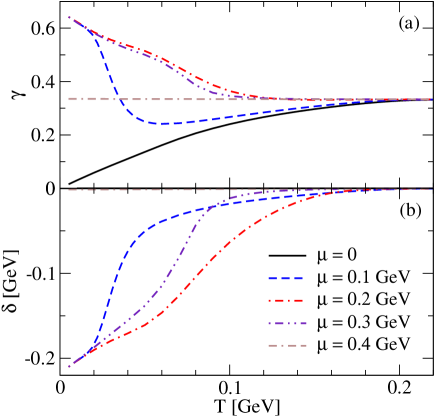
Figure 19: The coefficients $\gamma$ (a) and $\delta$ (b) as functions of the temperature for various values of the chemical potential.

Using Eqs. (82), (92), (93), (96) and (B) we find for the heat capacity

$$c_{V}=\frac{N_{c}N_{f}}{\pi^{2}T^{2}}\int_{0}^{\infty}p^{2}dpE_{p}[(E_{p}-\mu^{*})n^{+}(1-n^{+})$$

$$+(E_{p}+\mu^{*})n^{-}(1-n^{-})].$$ (105)

Finally, substituting Eqs. (98)–(100) and (B) into Eqs. (80) and (81) we obtain

$$\gamma = \frac{\int_{0}^{\infty}p^{4}dp(3E_{p})^{-1}[(E_{p}-\mu^{*})n^{+}(1-n^{+})+(E_{p}+\mu^{*})n^{-}(1-n^{-})]}{\int_{0}^{\infty}p^{2}dpE_{p}[(E_{p}-\mu^{*})n^{+}(1-n^{+})+(E_{p}+\mu^{*})n^{-}(1-n^{-})]},$$ (106)

$$\delta = \frac{\int_{0}^{\infty}p^{4}dp(3E_{p})^{-1}[(E_{p}-\mu^{\star})n^{+}(1-n^{+})+(E_{p}+\mu^{\star})n^{-}(1-n^{-})]}{\int_{0}^{\infty}p^{2}dp[(E_{p}-\mu^{\star})n^{+}(1-n^{+})-(E_{p}+\mu^{\star})n^{-}(1-n^{-})]}.$$ (107)

Equations (103), (104), (106) and (107) imply that $\mu^{*},\mu^{\star}$ and $\delta$ are odd and $\gamma$ - even functions of the chemical potential. The thermodynamic quantities $\gamma$ and $\delta$ given by Eqs. (106) and (107) are shown in Fig. 19. We find that $\gamma$ tends to a constant value $\gamma=1/3$ at high temperatures and chemical potentials. In $T\to 0$ limit $\gamma\to 0$ for $\mu=0$ and $\gamma\to 2/3$ for intermediate values of the chemical potential $T\ll\mu<m(T=0)$. Note that in the limit of vanishing chemical potential $\gamma=s/c_{V}$ coincides with the sound speed, which makes clear the high-temperature asymptotics of $\gamma$. We find also that $\delta$ is numerically negligible compared to the typical energy scales for the whole temperature-density range of interest. It vanishes asymptotically at high temperatures and densities, but tends to a constant limit $\delta\to-2m(T=0)/3\simeq 0.22$ GeV at $T\to 0$ if $m(T=0)>\mu\gg T$. In the chiral limit $m=0$ above the critical temperature $T_{c}$, and we find from Eqs. (B), (106) and (107) constant values $\gamma=1/3$ and $\delta=0$.

References

- (1) P. Danielewicz and M. Gyulassy, Dissipative phenomena in quark-gluon plasmas, Phys. Rev. D 31 (1985) 53–62.
- (2) P. K. Kovtun, D. T. Son and A. O. Starinets, Viscosity in Strongly Interacting Quantum Field Theories from Black Hole Physics, Physical Review Letters 94 (2005) 111601, [hep-th/0405231].
- (3) E. Lifshitz and L. Pitaevski, Physical Kinetics. Butterworth-Heinemann, Oxford, 1981.
- (4) S. Weinberg, Entropy Generation and the Survival of Protogalaxies in an Expanding Universe, ApJ 168 (1971) 175.
- (5) A. Hosoya and K. Kajantie, Transport coefficients of QCD matter, Nuclear Physics B 250 (1985) 666–688.
- (6) P. Arnold, Ç. Doǧan and G. D. Moore, Bulk viscosity of high-temperature QCD, Phys. Rev. D 74 (2006) 085021, [hep-ph/0608012].
- (7) G. D. Moore and O. Saremi, Bulk viscosity and spectral functions in QCD, Journal of High Energy Physics 9 (2008) 015, [0805.4201].
- (8) J.-W. Chen, Y.-F. Liu, Y.-K. Song and Q. Wang, Shear and bulk viscosities of a weakly coupled quark gluon plasma with finite chemical potential and temperature: Leading-log results, Phys. Rev. D 87 (2013) 036002, [1212.5308].
- (9) H. B. Meyer, Calculation of the Bulk Viscosity in SU(3) Gluodynamics, Physical Review Letters 100 (2008) 162001, [0710.3717].
- (10) K. Paech and S. Pratt, Origins of bulk viscosity in relativistic heavy ion collisions, Phys. Rev. C 74 (2006) 014901, [nucl-th/0604008].
- (11) K. Dusling and T. Schäfer, Bulk viscosity, particle spectra, and flow in heavy-ion collisions, Phys. Rev. C 85 (2012) 044909, [1109.5181].
- (12) K. Rajagopal and N. Tripuraneni, Bulk viscosity and cavitation in boost-invariant hydrodynamic expansion, Journal of High Energy Physics 3 (2010) 18, [0908.1785].
- (13) F. Karsch, D. Kharzeev and K. Tuchin, Universal properties of bulk viscosity near the QCD phase transition, Physics Letters B 663 (2008) 217–221, [0711.0914].
- (14) G. Aarts, Transport and spectral functions in high-temperature QCD, PoS LAT2007 (2007) 001, [0710.0739].
- (15) C. Sasaki and K. Redlich, Transport coefficients near chiral phase transition, Nuclear Physics A 832 (2010) 62–75, [0811.4708].
- (16) P. Chakraborty and J. I. Kapusta, Quasiparticle theory of shear and bulk viscosities of hadronic matter, Phys. Rev. C 83 (2011) 014906, [1006.0257].
- (17) V. Chandra, Bulk viscosity of anisotropically expanding hot QCD plasma, Phys. Rev. D 84 (2011) 094025, [1107.1195].
- (18) A. Dobado, F. J. Llanes-Estrada and J. M. Torres-Rincon, Bulk viscosity and energy-momentum correlations in high energy hadron collisions, European Physical Journal C 72 (2012) 1873, [1101.1801].
- (19) R. Marty, E. Bratkovskaya, W. Cassing, J. Aichelin and H. Berrehrah, Transport coefficients from the Nambu-Jona-Lasinio model for , Phys. Rev. C88 (2013) 045204, [1305.7180].
- (20) F. Werner and Y. Castin, Unitary gas in an isotropic harmonic trap: Symmetry properties and applications, Phys. Rev. A 74 (2006) 053604, [cond-mat/0607821].
- (21) D. T. Son, Vanishing Bulk Viscosities and Conformal Invariance of the Unitary Fermi Gas, Physical Review Letters 98 (2007) 020604, [cond-mat/0511721].
- (22) T. Enss, R. Haussmann and W. Zwerger, Viscosity and scale invariance in the unitary Fermi gas, Annals of Physics 326 (2011) 770–796, [1008.0007].
- (23) K. Dusling and T. Schäfer, Bulk Viscosity and Conformal Symmetry Breaking in the Dilute Fermi Gas near Unitarity, Physical Review Letters 111 (2013) 120603.
- (24) R. Kubo, Statistical-Mechanical Theory of Irreversible Processes. I, Journal of the Physical Society of Japan 12 (1957) 570–586.
- (25) D. Zubarev, V. Morozov and G. Röpke, Statistical Mechanics of Nonequilibrium Processes. John Wiley & Sons, 1997.
- (26) E. Quack and S. P. Klevansky, Effective 1/Nc expansion in the Nambu-Jona-Lasinio model, Phys. Rev. C 49 (1994) 3283–3288.
- (27) M. Iwasaki, H. Ohnishi and T. Fukutome, Shear viscosity of the quark matter, Journal of Physics G Nuclear Physics 35 (2008) 035003, [hep-ph/0703271].
- (28) W. M. Alberico, S. Chiacchiera, H. Hansen, A. Molinari and M. Nardi, Shear viscosity and entropy of quark matter, European Physical Journal A 38 (2008) 97–103, [0707.4442].
- (29) R. Lang and W. Weise, Shear viscosity from Kubo formalism: NJL model study, European Physical Journal A 50 (2014) 63.
- (30) R. Lang, N. Kaiser and W. Weise, Shear viscosities from Kubo formalism in a large-Nc Nambu-Jona-Lasinio model, European Physical Journal A 51 (2015) 127.
- (31) R. Lang, Shear Viscosities from Kubo Formalism in Large- Nambu–Jona-Lasinio Model. Doctoral Dissertation. Technische Universität München, 2015.
- (32) S. Ghosh, T. C. Peixoto, V. Roy, F. E. Serna and G. Krein, Shear and bulk viscosities of quark matter from quark-meson fluctuations in the Nambu-Jona-Lasinio model, Phys. Rev. C 93 (2016) 045205, [1507.08798].
- (33) S.-S. Xiao, P.-P. Guo, L. Zhang and D.-F. Hou, Bulk viscosity of hot dense Quark matter in the PNJL model, Chinese Physics C 38 (2014) 054101, [1306.3842].
- (34) A. Harutyunyan, D. H. Rischke and A. Sedrakian, Transport coefficients of two-flavor quark matter from the Kubo formalism, Phys. Rev. D 95 (2017) 114021, [1702.04291].
- (35) M. G. Alford, M. Braby, S. Reddy and T. Schäfer, Bulk viscosity due to kaons in color-flavor-locked quark matter, Phys. Rev. C 75 (2007) 055209, [nucl-th/0701067].
- (36) B. A. Sa’d, I. A. Shovkovy and D. H. Rischke, Bulk viscosity of spin-one color superconductors with two quark flavors, Phys. Rev. D 75 (2007) 065016, [astro-ph/0607643].
- (37) B. A. Sa’d, I. A. Shovkovy and D. H. Rischke, Bulk viscosity of strange quark matter: Urca versus nonleptonic processes, Phys. Rev. D 75 (2007) 125004, [astro-ph/0703016].
- (38) H. Dong, N. Su and Q. Wang, Baryon number conservation and enforced electric charge neutrality for bulk viscosity in quark matter, Phys. Rev. D 75 (2007) 074016, [astro-ph/0702104].
- (39) M. G. Alford, M. Braby and A. Schmitt, Bulk viscosity in kaon-condensed color flavor-locked quark matter, Journal of Physics G Nuclear Physics 35 (2008) 115007, [0806.0285].
- (40) X.-G. Huang, M. Huang, D. H. Rischke and A. Sedrakian, Anisotropic hydrodynamics, bulk viscosities, and r-modes of strange quark stars with strong magnetic fields, Phys. Rev. D 81 (2010) 045015, [0910.3633].
- (41) I. A. Shovkovy and X. Wang, Bulk viscosity in the nonlinear and anharmonic regimes of strange quark matter, New Journal of Physics 13 (2011) 045018, [1012.0354].
- (42) J. Berdermann, D. Blaschke, T. Fischer and A. Kachanovich, Neutrino emissivities and bulk viscosity in neutral two-flavor quark matter, Phys. Rev. D 94 (2016) 123010, [1609.05201].
- (43) L. I. Mandelstam and M. A. Leontovich, Zh. Exp. Theor. Fiz. 7 (1937) 438.
- (44) E. E. Kolomeitsev and D. N. Voskresensky, Viscosity of neutron star matter and r -modes in rotating pulsars, Phys. Rev. D 91 (2015) 025805.
- (45) R. Horsley and W. Schoenmaker, Quantum field theories out of thermal equilibrium. (I). General considerations, Nuclear Physics B 280 (1987) 716–734.
- (46) X.-G. Huang, A. Sedrakian and D. H. Rischke, Kubo formulas for relativistic fluids in strong magnetic fields, Annals of Physics 326 (2011) 3075–3094, [1108.0602].
- (47) S. P. Klevansky, The Nambu-Jona-Lasinio model of quantum chromodynamics, Reviews of Modern Physics 64 (1992) 649–708.
- (48) M. Buballa, NJL-model analysis of dense quark matter [review article], Phys. Rep. 407 (2005) 205–376, [hep-ph/0402234].