Global hard thresholding algorithms for joint sparse image representation and denoising

Abstract

Sparse coding of images is traditionally done by cutting them into small patches and representing each patch individually over some dictionary given a pre-determined number of nonzero coefficients to use for each patch. In lack of a way to effectively distribute a total number (or global budget) of nonzero coefficients across all patches, current sparse recovery algorithms distribute the global budget equally across all patches despite the wide range of differences in structural complexity among them. In this work we propose a new framework for joint sparse representation and recovery of all image patches simultaneously. We also present two novel global hard thresholding algorithms, based on the notion of variable splitting, for solving the joint sparse model. Experimentation using both synthetic and real data shows effectiveness of the proposed framework for sparse image representation and denoising tasks. Additionally, time complexity analysis of the proposed algorithms indicate high scalability of both algorithms, making them favorable to use on large megapixel images.

1 Introduction

In recent years a large number of algorithms have been developed for approximately solving the NP-hard sparse representation problem

$$\underset{\mathbf{x}}{\mbox{minimize}} \,\,\|\mathbf{D}\mathbf{x}-\mathbf{y}\|_{2}^{2}$$ (1)

subject to $$\,\,\|\mathbf{x}\|_{0}\leq s,$$

where $\mathbf{y}$ is a signal of dimension $N\times 1$, $\mathbf{D}$ is an $N\times L$ dictionary, $\mathbf{x}$ is an $L\times 1$ coefficient vector, and $\|\cdot\|_{0}$ denotes the $\ell_{0}$ norm that counts the number of nonzero entries in a vector (or matrix). These approaches can be roughly divided into three categories. First, greedy pursuit approaches such as the popular Orthogonal Matching Pursuit (OMP) algorithm [1, 2] which sequentially adds new atoms (or dictionary elements) to a signal representation in a greedy fashion until the entire budget of $s$ nonzero coefficients is used. Second, convex relaxation approaches like the Fast Iterative Shrinkage Thresholding Algorithm (FISTA) [3] wherein the $\ell_{0}$ norm of the coefficient vector $\mathbf{x}$ is appropriately weighted, brought up to the objective function, and replaced with an $\ell_{1}$ norm. This convex relaxation of the sparse representation problem in (1) is then solved via accelerated proximal gradient. Lastly, hard thresholding approaches such as the Accelerated Iterative Hard Thresholding (AIHT) algorithm [4] which approximately solves (1) by projected gradient descent onto the nonconvex set of $s$-sparse vectors given by $\left\{\mathbf{x}\in\mathbb{R}^{L}\,|\,\|\mathbf{x}\|_{0}\leq s\right\}$.

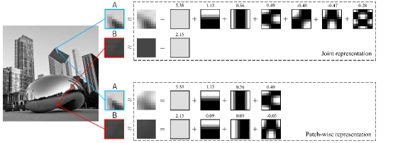
Figure 1: (top) Joint and (bottom) patch-wise representations of two $8\times 8$ patches using a total budget of $8$ DCT atoms, where the respective coefficient is written on top of each atom. Comparing the reconstructed patches in the bottom panel to those in the top panel shows an intangible improvement gained by adding more atoms to the representation of patch B at the expense of a significant deterioration in reconstructing patch A. This simple observation justifies the intuitive choice of allocating a larger number of atoms to represent patches with more complex structure, as well as algorithms for automatically making smart global budget allocations.

Greedy pursuit and convex relaxation approaches have received significant attention from researchers in signal and image processing (see e.g., [5, 2, 1, 3, 6]). However, several recent works have suggested that hard thresholding routines not only have strong recovery guarantees, but in practice can outperform greedy pursuit or convex relaxation approaches, particularly in compressive sensing [7, 8] applications, both in terms of efficacy and computation time [4, 9, 10]. Current hard thresholding routines that are proposed to solve the general constrained optimization problem

$$\underset{\mathbf{x}}{\mbox{minimize}} \,\,f\left(\mathbf{x}\right)$$ (2)

subject to $$\,\,\,\mathbf{x}\in\mathcal{T},$$

are largely based on the projected gradient method, wherein at the $k^{th}$ iteration a gradient descent step is taken in the objective function $f$ and is then adjusted via an appropriate operator as

$$\mathbf{x}^{k}=P_{\mathcal{T}}\left(\mathbf{x}^{k-1}-\alpha_{k}\nabla f\left(\mathbf{x}^{k-1}\right)\right).$$ (3)

Here the gradient step $\mathbf{x}^{k-1}-\alpha_{k}\nabla f\left(\mathbf{x}^{k-1}\right)$, where $\alpha_{k}$ is an appropriately chosen step-length, is transformed by the projection operator $P_{\mathcal{T}}\left(\cdot\right)$ so that each step in the procedure remains in the problem’s given constraint set $\mathcal{T}$. Denoting by $\mathcal{H}_{s}\left(\cdot\right)$ the projection onto the $s$-sparse set, we have

$$\mathcal{H}_{s}\left(\mathbf{y}\right)=\underset{\left\|\mathbf{x}\right\|_{0}\leq s}{\mbox{argmin}} \,\,\|\mathbf{x}-\mathbf{y}\|_{2}^{2}$$ (4)

where $\mathcal{H}_{s}\left(\mathbf{y}\right)$ is a vector of equal length to $\mathbf{y}$ wherein we keep only the top $s$ (in magnitude) entries of $\mathbf{y}$, and set the remaining elements to zero. With this notation, popular hard thresholding approaches [11, 9, 4, 10] for solving (1) take projected gradient steps of the form

$$\mathbf{x}^{k}=\mathcal{H}_{s}\left(\mathbf{x}^{k-1}-\alpha_{k}\mathbf{D}^{T}\left(\mathbf{D}\mathbf{x}^{k-1}-\mathbf{y}\right)\right).$$ (5)

Since the $s$-sparse set is nonconvex one might not expect projected gradient to converge at all, let alone to a sufficiently low objective value. However projected gradient in this instance is in fact provably convergent when the dictionary $\mathbf{D}$ satisfies various forms of a Restricted Isometry Property (RIP) [12], i.e., if $\mathbf{D}$ satisfies

$$\left(1-\delta_{s}\right)\left\|\mathbf{x}\right\|_{2}^{2}\leq\left\|\mathbf{D}\mathbf{x}\right\|_{2}^{2}\leq\left(1+\delta_{s}\right)\left\|\mathbf{x}\right\|_{2}^{2}$$ (6)

for all $s$-sparse vectors $\mathbf{x}$ and for some $\delta_{s}\in\left(0,1\right)$. Such a matrix is used almost exclusively in compressive sensing applications. Analogous projected gradient methods have been successfully applied to the low-rank matrix completion problem [13], where hard thresholding is performed on singular values as opposed to entries of a matrix itself, and has also been shown to be theoretically and practically superior to standard convex relaxation approaches which invoke the rank-convexifying surrogate, the nuclear norm [14], when RIP conditions hold for the problem. It must be noted that while these algorithms have mathematically guaranteed convergence for RIP-based problems, it is unclear how well they contend on the plethora of other instances of (1) where the matrix $\mathbf{D}$ does not necessarily hold an RIP (e.g., image denoising and deblurring [15, 16], super-resolution [17, 18], sparse coding [19]).

1.1 Joint sparse representation model

Figure 2: With an algorithm for solving the global sparse representation problem we can automatically distribute a global budget where it really needs to be: on high frequency areas of an image. (left) The original image. (middle) The heatmap generated by counting the number of atoms used in reconstructing each patch. (right) The reconstructed image with a root mean square error of less than $1$.

In many image processing applications large or even moderate sized images are cut into small image patches (or blocks), and then one wants to sparsely represent a large number of patches $\left\{\mathbf{y}_{p}\right\}_{p=1}^{P}$ together, given a global budget $S$ for the total number of nonzero coefficients to use. This ideally requires the user to decide on the individual per patch budget $s_{p}$ for each of the $P$ patches in a way to ensure that $\underset{p}{\sum}s_{p}\leq S$. Because this global budget allocation problem seems difficult to solve, in practice a fixed $s=\lfloor\frac{S}{P}\rfloor$ is typically chosen for all patches, even though this choice results in a suboptimal distribution of the global budget considering the wide range of differences in structural complexity across the patches. This is particularly the case with natural images wherein patches vary extremely in terms of texture, structure, and frequency content. We illustrate this observation through a simple example in Figure 1 where two $8\times 8$ patches taken from an image are sparsely represented over the $64\times 64$ Discrete Cosine Transform (DCT) dictionary. One of the patches (patch B in Figure 1) is rather flat and can be represented quite well using only one atom from the DCT dictionary while the other more structurally complex patch (patch A) requires at least $7$ atoms in order to be represented equally well in terms of reconstruction error. Notice that the naive way of distributing a total of $8$ nonzero coefficients equally across both patches ($4$ atoms per patch) would adversely affect the representation of the more complex patch with no tangible improvement in the representation of the flatter one.

This observation motivates introduction of the joint sparse representation problem, where local patch-wise budgets can be determined automatically via solving

$$\underset{\mathbf{X}}{\mbox{minimize}} \,\,\|\mathbf{D}\mathbf{X}-\mathbf{Y}\|_{F}^{2}$$ (7)

subject to $$\,\,\|\mathbf{X}\|_{0}\leq S,$$

where we have concatenated all signals $\left\{\mathbf{y}_{p}\right\}_{p=1}^{P}$ into an $N\times P$ matrix $\mathbf{Y}$, $\mathbf{X}$ is the corresponding coefficient matrix of size $L\times P$, and $\|\cdot\|_{F}$ denotes the Frobenius norm. If this problem could be solved efficiently, the issue of how to distribute the budget $S$ across all $P$ patches would be taken care of automatically, alleviating the painstaking per patch budget tuning required when applying (1) to each individual patch. Note that one could concatenate all columns in the matrix $\mathbf{X}$ into a single vector and then use any of the patch-wise algorithms designed for solving (1). This solution however is not practically feasible due to the potentially large size of $\mathbf{X}$.

1.2 Proposed approaches

The hard thresholding approaches described in this work for solving (7) are based on the notion of variable splitting as well as two classic approaches to constrained numerical optimization. More specifically, in this work we present two scalable hard thresholding approaches for approximately solving the joint sparse representation problem in (7). The first approach, based on variable splitting and the Quadratic Penalty Method (QPM) [20], is a provably convergent method while the latter employs a heuristic form of the Alternating Direction Method of Multipliers (ADMM) framework [21]. While ADMM is often applied to convex optimization problems (where it is provably convergent), our experiments add to the growing body of work showing that ADMM can be a highly effective empirical heuristic method for nonconvex optimization problems.

To illustrate what can be achieved by solving the joint model in (7), we show in Figure 2 the result of applying our first global hard thresholding algorithm to sparsely represent a megapixel image. Specifically, we sparsely represent a gray-scale image of size $1024\times 1024$ over a $64\times 100$ overcomplete Discrete Cosine Transform (DCT) dictionary using a fixed global budget of $S=20\times P$, where $P$ is the number of non-overlapping $8\times 8$ patches which constitute the original image. We also keep count of the number of atoms used in reconstructing each patch, that is the count $\left\|\mathbf{x}_{p}\right\|_{0}$ of nonzero coefficients in the final representation $\mathbf{D}\mathbf{x}_{p}$ for each patch $\mathbf{y}_{p}$, and form a heatmap of the same size as the original image in order to provide initial visual verification that our algorithm properly distributes the global budget. In the heatmap the brighter the patch color the more atoms are assigned in reconstructing it. As can be seen in the middle panel of Figure 2, our algorithm appears to properly allocate fractions of the budget to high frequency portions of the image.

The remainder of this work is organized as follows: in the next Section we derive both Global Hard Thresholding (GHT) algorithms, referred to as GHT-QPM and GHT-ADMM hereafter, followed by a complete time complexity analysis of each algorithm. Then in Section 3 we discuss the experimental results of applying both algorithms to sparse image representation and denoising tasks. Finally we conclude this paper in Section 4 with reflections and thoughts on future work.

2 Global Hard Thresholding

In this work we introduce two new hard thresholding algorithms that are effectively applied to the joint sparse representation problem in (7). Both methods are based on variable-splitting, as opposed to the projected gradient technique, and unlike the methods discussed in Section 1 do not rely on any kind of RIP condition on the dictionary matrix $\mathbf{D}$.

2.1 GHT-QPM

The first method we introduce is based on variable splitting and the Quadratic Penalty Method (QPM). By splitting the optimization variable we may equivalently rewrite the joint sparse representation problem from equation (7) as

$$\underset{\mathbf{X},\mathbf{Z}}{\mbox{minimize}} \,\,\|\mathbf{D}\mathbf{X}-\mathbf{Y}\|_{F}^{2}$$ (8)

subject to $$\,\,\|\mathbf{Z}\|_{0}\leq S$$

$$\,\,\mathbf{X}=\mathbf{Z}.$$

Using QPM we may relax this version of the problem by bringing the equality constraint to the objective in weighted and squared norm as

$$\underset{\mathbf{X},\mathbf{Z}}{\mbox{minimize}} \,\,\|\mathbf{D}\mathbf{X}-\mathbf{Y}\|_{F}^{2}+\rho\|\mathbf{X}-\mathbf{Z}\|_{F}^{2}$$ (9)

subject to $$\,\,\|\mathbf{Z}\|_{0}\leq S,$$

where $\rho>0$ controls how well the equality constraint holds. A simple alternating minimization approach can then be applied to solving this relaxed form of the joint problem. Specifically, at the $k^{th}$ step we solve for the following two closed form update steps first by minimizing the objective of (9) with respect to $\mathbf{X}$ with $\mathbf{Z}$ fixed at its previous value $\mathbf{Z}^{k-1}$, as

$$\mathbf{X}^{k}=\underset{\mathbf{X}}{\mbox{argmin}}\|\mathbf{D}\mathbf{X}-\mathbf{Y}\|_{F}^{2}+\rho\|\mathbf{X}-\mathbf{Z}^{k-1}\|_{F}^{2},$$ (10)

which can be written in closed form as the solution to the linear system

$$\left(\mathbf{D}^{T}\mathbf{D}+\rho\mathbf{I}\right)\mathbf{X}=\mathbf{D}^{T}\mathbf{Y}+\rho\mathbf{Z}^{k-1},$$ (11)

and can be solved for in closed form as

$$\mathbf{X}^{k}=\left(\mathbf{D}^{T}\mathbf{D}+\rho\mathbf{I}\right)^{-1}\left(\mathbf{D}^{T}\mathbf{Y}+\rho\mathbf{Z}^{k-1}\right).$$ (12)

However we note that in practice such a linear system is almost never solved by actually inverting the matrix $\mathbf{D}^{T}\mathbf{D}+\rho\mathbf{I}$, since solving the linear system directly via numerical linear algebra methods is significantly more efficient. Moreover, since in our case this matrix remains unchanged throughout the iterations significant additional computation savings can be achieved by catching a Cholesky factorization of $\mathbf{D}^{T}\mathbf{D}+\rho\mathbf{I}$. We discuss this further in Subsection 2.3.

Next, minimizing the objective of (9) with respect to $\mathbf{Z}$ gives the projection problem

$$\mathbf{Z}^{k}=\underset{\left\|\mathbf{Z}\right\|_{0}\leq S}{\mbox{argmin}}\|\mathbf{Z}-\mathbf{X}^{k}\|_{F}^{2},$$ (13)

to which the solution is a hard thresholded version of $\mathbf{X}^{k}$ given explicitly as $\mathbf{Z}^{k}=\mathcal{H}_{S}\left(\mathbf{X}^{k}\right)$. Taking both updates together, the complete version of GHT-QPM is given in Algorithm 1.

Inputs: Dictionary $\mathbf{D}$, signal concatenation matrix $\mathbf{Y}$, penalty parameter $\rho>0$, global budget $S$, and initialization for $\mathbf{Z}^{0}$

Output: Final coefficient matrix $\mathbf{Z}^{k}$

 

$k=1$

Find Cholesky factorization of  $\mathbf{D}^{T}\mathbf{D}+\rho\mathbf{I}\rightarrow\mathbf{C}\mathbf{C}^{T}$

Pre-compute $\mathbf{\mathbf{W}=D}^{T}\mathbf{Y}$

While convergence criterion not met

Solve $\mathbf{CJ}=\mathbf{\mathbf{W}}+\rho\mathbf{Z}^{k-1}$ for $\mathbf{J}$ via forward substitution

Solve $\mathbf{C}^{T}\mathbf{X}^{k}=\mathbf{\mathbf{J}}$ for $\mathbf{X}^{k}$ via backward substitution

Find the projection $\mathbf{Z}^{k}=\mathcal{H}_{S}\left(\mathbf{X}^{k}\right)$

$k\leftarrow k+1$

End

Algorithm 1 GHT-QPM

2.2 GHT-ADMM

We also introduce a second method for approximately solving the joint problem, which is a heuristic form of the popular Alternating Direction Method of Multipliers (ADMM). While developed close to a half a century ago, ADMM and other Lagrange multiplier methods in general have seen an explosion of recent interest in the machine learning and signal processing communities [21, 22]. While classically ADMM has been provably mathematically convergent for only convex problems, recent work has also proven convergence of the method for particular families of nonconvex problems (see e.g., [23, 24, 25, 26]). There has also been extensive successful use of ADMM as a heuristic method for highly nonconvex problems [24, 23, 27, 21, 28, 29, 30, 31]. It is in this spirit that we have applied ADMM to our nonconvex problem and, like these works, find it to provide excellent results empirically (see Section 3).

To achieve an ADMM algorithm for the joint problem we rewrite it by again introducing a surrogate variable $\mathbf{Z}$ as

$$\underset{\mathbf{X},\mathbf{Z}}{\mbox{minimize}} \,\,\|\mathbf{D}\mathbf{X}-\mathbf{Y}\|_{F}^{2}$$ (14)

subject to $$\,\,\|\mathbf{Z}\|_{0}\leq S$$

$$\,\,\mathbf{X}=\mathbf{Z}.$$

We then form the Augmented Lagrangian associated with this problem, given by

$$\begin{array}[]{c}\mathcal{L}\left(\mathbf{X},\mathbf{Z},\boldsymbol{\Lambda},\rho\right)=\|\mathbf{D}\mathbf{X}-\mathbf{Y}\|_{F}^{2}\\ +\rho\|\mathbf{X}-\mathbf{Z}\|_{F}^{2}+\left\langle\boldsymbol{\Lambda},\,\mathbf{X}-\mathbf{Z}\right\rangle\end{array}$$ (15)

where $\boldsymbol{\Lambda}$ is the dual variable, $\left\langle\cdot,\cdot\right\rangle$ returns the inner-product of its input matrices, and $\mathbf{Z}$ is constrained such that $\|\mathbf{Z}\|_{0}\leq S$. With ADMM we repeatedly take a single Gauss-Seidel sweep across the primal variables, minimizing $\mathcal{L}$ independently over $\mathbf{X}$ and $\mathbf{Z}$ respectively, followed by a single dual ascent step in $\boldsymbol{\Lambda}$. This gives the closed form updates for the two primal variables as

$$\mathbf{X}^{k}=\left(\mathbf{D}^{T}\mathbf{D}+\rho\mathbf{I}\right)^{-1}\left(\mathbf{D}^{T}\mathbf{Y}+\rho\mathbf{Z}^{k-1}-\boldsymbol{\Lambda}^{k-1}\right)$$ (16)

$$\begin{array}[]{c}\mathbf{Z}^{k}=\mathcal{H}_{S}\left[\mathbf{X}^{k}+\frac{1}{\rho}\boldsymbol{\Lambda}^{k-1}\right]\end{array}$$

Again the linear system in the $\mathbf{X}$ update is solved effectively via catched Cholesky factorization, and $\mathcal{H}_{S}\left(\cdot\right)$ is the hard thresholding operator. The associated dual ascent update step is then given by

$$\boldsymbol{\Lambda}^{k}=\boldsymbol{\Lambda}^{k-1}+\rho\left(\mathbf{X}^{k}-\mathbf{Z}^{k}\right).$$ (17)

For convenience we summarize the ADMM heuristic used in this paper in Algorithm 2.

Inputs: Dictionary $\mathbf{D}$, signal concatenation matrix $\mathbf{Y}$, penalty parameter $\rho>0$, global budget $S$, and initializations for $\mathbf{Z}^{0}$ and $\boldsymbol{\Lambda}^{0}$

Output: Final coefficient matrix $\mathbf{Z}^{k}$

 

$k=1$

Find Cholesky factorization of  $\mathbf{D}^{T}\mathbf{D}+\rho\mathbf{I}\rightarrow\mathbf{C}\mathbf{C}^{T}$

Pre-compute $\mathbf{\mathbf{W}=D}^{T}\mathbf{Y}$

While convergence criterion not met

Solve $\mathbf{CJ}=\mathbf{\mathbf{W}}+\rho\mathbf{Z}^{k-1}-\boldsymbol{\Lambda}^{k-1}$ for $\mathbf{J}$

Solve $\mathbf{C}^{T}\mathbf{X}^{k}=\mathbf{\mathbf{J}}$ for $\mathbf{X}^{k}$

Find the projection $\mathbf{Z}^{k}=\mathcal{H}_{S}\left(\mathbf{X}^{k}+\frac{1}{\rho}\boldsymbol{\Lambda}^{k-1}\right)$

Update the dual variable $\boldsymbol{\Lambda}^{k}=\boldsymbol{\Lambda}^{k-1}+\rho\left(\mathbf{X}^{k}-\mathbf{Z}^{k}\right)$

$k\leftarrow k+1$

End

Algorithm 2 GHT-ADMM

2.3 Time complexity analysis

In this Section we derive time complexities of both proposed algorithms. In what follows we assume that i) $L=2N$, that is the dictionary is two times overcomplete, and ii) the number of signals $P$ greatly dominates every other influencing parameter.

As can be seen in Algorithm 1, each iteration of GHT-QPM includes i) solving a linear system of equations to update $\mathbf{X}^{k}$, and ii) hard thresholding the solution to update $\mathbf{Z}^{k}$. In our implementation of GHT-QPM we pre-compute $\mathbf{D}^{T}\mathbf{Y}$ as well as the Cholesky factorization of the matrix $\mathbf{D}^{T}\mathbf{D}+\rho\mathbf{I}$ outside the loop and as a result, updating $\mathbf{X}^{k}$ can be done more cheaply via forward/backward substitutions inside the loop. Assuming $\mathbf{D}\in\mathbb{R}^{N\times 2N}$ and $\mathbf{Y}\in\mathbb{R}^{N\times P}$, construction of matrices $\mathbf{D}^{T}\mathbf{Y}$ and $\mathbf{D}^{T}\mathbf{D}+\rho\mathbf{I}$ require $4N^{2}P$ and $4N^{3}+2N$ operations, respectively. In our analysis we do not account for matrix (re)assignment operations that can be dealt with memory pre-allocation. Additionally, whenever possible we can take advantage of the symmetry of the matrices involved, as is for example the case when computing $\mathbf{D}^{T}\mathbf{D}+\rho\mathbf{I}$. Finally, considering $\frac{8}{3}N^{3}$ operations required for Cholesky factorization of $\mathbf{D}^{T}\mathbf{D}+\rho\mathbf{I}$, the outside-the-loop cost of GHT-QPM adds up to $4N^{2}P+\frac{20}{3}N^{3}+2N$, that is $\mathcal{O}(N^{2}P)$.

Now to compute the per iteration cost of GHT-QPM, the cost of hard thresholding operation must be added to the $8N^{2}P$ operations needed for forward and backward substitutions, as well as the $4NP$ operations required for computing $\mathbf{D}^{T}\mathbf{Y}+\rho\mathbf{Z}^{k}$. Luckily, we are only interested in finding the $S$ largest (in magnitude) elements of $\mathbf{X}^{k}$, where $S$ is typically much smaller than $2NP$ - the total number of elements in $\mathbf{X}^{k}$. A number of efficient algorithms have been proposed to find the $S$ largest (or smallest) elements in an array, that run in linear time [32, 33, 34]. In particular Hoare’s selection algorithm [32], also known as quickselect, runs in $\mathcal{O}(NP)$. Combined together, the per iteration cost of GHT-QPM adds up to $8N^{2}P+4NP+\mathcal{O}(NP)$, that is again $\mathcal{O}(N^{2}P)$.

The time complexity analysis of GHT-ADMM is essentially similar to that of GHT-QPM, with a few additional steps: subtraction of $\boldsymbol{\Lambda}^{k-1}$ from $\mathbf{D}^{T}\mathbf{Y}+\rho\mathbf{Z}^{k}$ in updating $\mathbf{X}^{k}$ which takes $2NP$ operations, addition of $\frac{1}{\rho}\boldsymbol{\Lambda}^{k-1}$ to $\mathbf{X}^{k}$ in updating $\mathbf{Z}^{k}$ which requires $4NP$ more operations, and finally the dual variable update $\boldsymbol{\Lambda}^{k}\leftarrow\boldsymbol{\Lambda}^{k-1}+\rho\left(\mathbf{X}^{k}-\mathbf{Z}^{k}\right)$ which adds $6NP$ operations to the per iteration cost of GHT-ADMM. Despite these additional computations, solving the two linear systems remains the most expensive step, and hence the time complexity of GHT-ADMM is $\mathcal{O}(N^{2}P)$, akin to that of GHT-QPM.

3 Experiments

In this Section we present the results of applying our proposed global hard thresholding algorithms to several sparse representation and recovery problems. For both GHT-QPM and GHT-ADMM and for all synthetic and real experiments we kept $\rho$ fixed at $\rho=0.1$, however we found that both algorithms are fairly robust to the choice of this parameter. We also initialized both $\mathbf{Z}$ and $\mathbf{\boldsymbol{\Lambda}}$ as zero matrices. As a stopping condition, we ran both algorithms until subsequent differences of the RMSE value $\sqrt{\frac{\left\|\mathbf{D}\mathbf{Z}^{k}-\mathbf{Y}\right\|_{F}^{2}}{P}}$, where $P$ is again the total number of patches, was less than $10^{-5}$. In all experiments we compare our approach with popular approaches that work on the patch level: the Orthogonal Matching Pursuit (OMP) algorithm as implemented in the SparseLab package [35], the Accelerated Iterative Hard Thresholding (AIHT) algorithm [4], and the Compressive Sampling Matching Pursuit (CoSaMP) algorithm [36]. All experiments were run in MATLAB R2012b on a machine with a 3.40 GHz Intel Core i7 processor and 16 GB of RAM.

3.1 Experiment on synthetic data

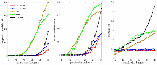
Figure 3: Comparison of our methods with patch-wise greedy and hard thresholding approaches on synthetic data, in terms of (left) support mismatch ratio, (middle) reconstruction error, and (right) computation time. The results are plotted for $s=5...30$.

We begin with a simple synthetic experiment where we create an overcomplete matrix $\mathbf{D}$ of size $100\times 200$ whose entries are generated from a Gaussian distribution (with zero mean and standard deviation of $0.1$). We then generate $P=100$ $s$-sparse signals $\mathbf{x}_{p}$ for $p=1...100$ each consisting of $s$ nonzero entries taking on the values $\pm 1$ uniformly. We then set $\mathbf{y}_{p}=\mathbf{D}\mathbf{x}_{p}$ for all $p$ and either solve $100$ instances of the local problem according to the model in (1) using a patch-wise competitor algorithm, or by our methods using the joint model in (7) where the global budget $S$ is set to $100s$. This procedure is repeated for each value of $s$ in the range of $s=5...30$ and with $5$ different dictionaries generated as described above. Finally the average support mismatch ratio, reconstruction error, and computation time are reported and displayed in Figure 3. Of these three criteria, the first two measure how close the recovered solution is to the true solution while the last one captures each algorithm’s runtime and how it varies by changing the sparsity level $s$. More specifically, support mismatch ratio measures the distance between the support of the true solution $\mathbf{X}$ denoted by $\mathcal{A}$ and that of the recovered solution $\mathbf{Z}^{K}$ denoted by $\mathcal{B}$, and is given by [37]

$$\textrm{mismatch ratio}=\frac{\textrm{max}\left\{\left|\mathcal{A}\right|,\,\left|\mathcal{B}\right|\right\}-\left|\mathcal{A}\cap\mathcal{B}\right|}{\textrm{max}\left\{\left|\mathcal{A}\right|,\,\left|\mathcal{B}\right|\right\}}.$$ (18)

Here $\left|\mathcal{A}\right|=\left|\mathcal{B}\right|=100s$, and a mismatch ratio of zero indicates perfect recovery of the true support. Reconstruction error (or RMSE) on the other hand measures how close the recovered representation $\mathbf{DZ}^{k}$ is to $\mathbf{Y}$. As can be seen in Figure 3, both GHT-QPM and GHT-ADMM are competitive with the best of the patch-wise algorithms in all three of these categories. Interestingly, while both global hard thresholding algorithms match the leading algorithm (CoSaMP) in terms of support mismatch ratio and reconstruction error, they also match the algorithm with best computation time (OMP). Therefore these experiments seem to indicate that global hard thresholding provides the best of both worlds: algorithms with high accuracy and low computation time. It is also worth noting that unlike the competitors, the computation time of both proposed algorithms do not increase as the per patch sparsity level $s$ increases, as expected from the time complexity analysis in Subsection 2.3 of Section 2. Finally, note that in this experiment we did not take full advantage of the power of the joint model in (7) over the patch-wise model in (1) since all the synthetic patches were created using the same number $s$ of dictionary atoms, and this number was given to all patch-wise algorithms. However the assumption that all patches taken from natural images could be well represented using the same number of atoms does not typically hold, and as we will see next the experiments on real data show that our global methods significantly outperform patch-wise algorithms in terms of reconstruction error.

3.2 Sparse representation of megapixel images

Here we perform a series of experiments on sparse representation of large megapixel images, using those images displayed in Figure 4. In the first set of experiments we compare GHT-QPM and GHT-ADMM to OMP, AIHT, and CoSaMP in terms of their ability to sparsely represent these images. This experiment illustrates the surprising efficacy and scalability of our global hard thresholding approaches.

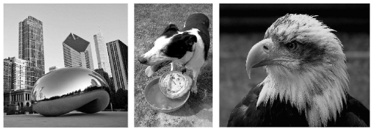
Figure 4: Megapixel gray scale images used for sparse representation and denoising experiments. From left to right: Chicago; size: $1024\times 1024$, hot-dog; size: $800\times 1360$, and eagle; size: $1200\times 880$.

Decomposing each image into $P$ non-overlapping $8\times 8$ patches, this data is columnized into $64\times 1$ vectors and concatenated into a $64\times P$ matrix referred to as $\mathbf{Y}$. We then learn sparse representations for these image patches over a $64\times 100$ overcomplete DCT dictionary. Specifically, we run each patch-wise algorithm using an average per patch budget of $s=\nicefrac{{S}}{{P}}$ nonzero coefficients for $s$ in a range of $5$ to $30$ in increments of $1$. We then run both global algorithms on the entire data set $\mathbf{Y}$ using the global budget $S$.

Figure 5 displays the results of these experiments on the megapixel images from Figure 4, including final root mean squared errors and runtimes of the associated algorithms. In all instances both of our global methods significantly outperform the various patch-wise methods in terms of RMSE over the entire budget range. For example, with a patch-wise budget of $\nicefrac{{S}}{{P}}=10$ the RMSE of our algorithms range between $78\%$ and $350\%$ lower than the nearest competitor. This major difference in reconstruction error lends credence to the claim that GHT algorithms effectively distribute the global budget across all patches of the megapixel image. While not overly surprising given the wealth of work on ADMM heuristic algorithms (see Subsection 2.2 of Section 2), it is interesting to note that GHT-ADMM outperforms GHT-QPM (as well as all other competitors) in terms of RMSE. Moreover, the total computation time of our algorithms remain fairly stable across the range of budgets tested, while competitors’ runtimes can increase quite steeply as the nonzero budget is increased.

To compare visual quality of the images reconstructed by different algorithms, we show in Figure 6 the results obtained by OMP (the best competitor) and GHT-QPM (the inferior of our two proposed algorithms) using a total budget of $S=5P$ on one of test images. The close-up comparison between the two methods clearly shows the visual advantage gained by solving the joint model.

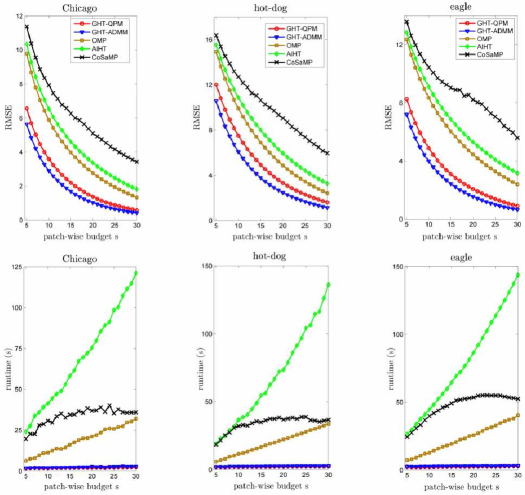
Figure 5: Comparison of our methods with patch-wise greedy and hard thresholding approaches on real data. (top panels) RMSE plotted as a function of patch-wise nonzero budget $s$ over a range of $5$ to $30$. Both GHT-QPM and GHT-ADMM significantly outperform the nearest competitor in terms of RMSE. (bottom panels) Computation time for the algorithms compared at each budget level. While the total runtime of competing algorithms increases substantially with the budget level, the run times of our algorithms remain stable across the range of tested budgets.

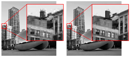
Figure 6: Close-up visual comparison of OMP (the best competitor) and GHT-QPM (the inferior of our two proposed algorithms). OMP (left) uses a per patch budget of $\nicefrac{{S}}{{P}}=5$ nonzeros while GHT-QPM (right) is given the equivalent global budget of $S=5P$.

3.3 Runtime and convergence on a million patches

So far in both synthetic and real sparse representation experiments we have kept the number of patches $P$ fixed and only varied the patch-wise budget $s$. It is also of practical interest to explore how the runtimes of patch-wise and global algorithms are affected when the number of patches increase while keeping a fixed patch-wise budget. To conduct this experiment we collect a set of $P$ random $8\times 8$ patches taken from a collection of natural images [38]. For each $P\in\left\{2^{10},\,2^{11},\,\ldots,2^{20}\right\}$ we then run all the algorithms keeping a fixed per patch budget of $s=\nicefrac{{S}}{{P}}=10$ and plot the computation times in Figure 7. As expected the runtime of both our algorithms are linear in $P$ (note that the scale on the x-axis is logarithmic). This Figure confirms that both GHT algorithms are highly scalable. As can be seen GHT-ADMM runs slightly slower than GHT-QPM which is consistent with our time complexity analysis.

Finally, we choose three global sparsity budgets such that an average of $s=5$, $10$, and $15$ atoms would be used per individual patch and run GHT-QPM and GHT-ADMM to resolve $10^{6}$ randomly selected patches. In Figure 8 we plot for each iteration $k=1...100$ the RMSE value. Note three observations: firstly, both algorithms have decreasing values of $\left\|\mathbf{D}\mathbf{Z}^{k}-\mathbf{Y}\right\|$ empirically, secondly that GHT-ADMM gives lower reconstruction errors compared to GHT-QPM across all budget levels, and third that within as few as just $10$ iterations both algorithms have converged.

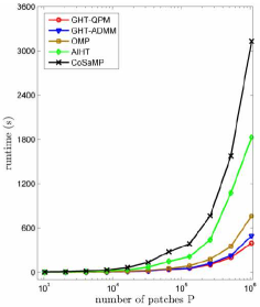
Figure 7: Runtime comparison of all patch-wise and global algorithms computed over a wide range ($2^{10}$ to $2^{20}$) of randomly selected $8\times 8$ patches.

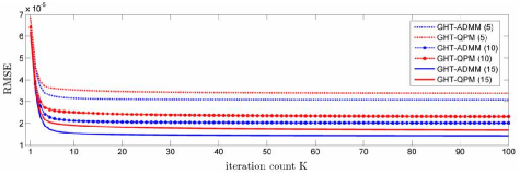
Figure 8: Change of RMSE over iteration count for GHT-QPM and GHT-ADMM. Three global budget levels are used: $S=5P$, $10P$, and $15P$.

3.4 Natural image denoising

In this next set of experiments, we add Gaussian noise to the images in Figure 4 and test the efficacy of our proposed methods for noise removal. More specifically, for a range of noise levels $\sigma=5$, $10$, $20$, $30$, and $40$ we add zero mean Gaussian noise with standard deviation $\sigma$ to these images, which are then as before decomposed into $P$ non-overlapping $8\times 8$ patches, each of which is columnized, and a $64\times P$ matrix $\mathbf{Y}$ is formed. Both of our global algorithms, GHT-QPM and GHT-ADMM, are then given this entire matrix to denoise along with a global budget of $S=10P$ nonzero coefficients. The competing algorithms are given the analogous patch-wise budgets of $\nicefrac{{S}}{{P}}=10$ nonzero coefficients, and process the image on the patch level. Noise removal results in terms of PSNR (in dB) are tabulated in Tables 1 through 3. For each noise level, PSNR of the best algorithm is boxed. Here we can see that both of our global methods significantly outperform patch-wise algorithms, particularly at low to moderate noise levels. For example, at a noise level of $\sigma=10$ our algorithms greatly outperform the nearest competitor on the images tested by $2.7$ to $4.9$ dB, and at $\sigma=15$ both global algorithms produce results at $1$ to $2.6$ dB lower than the nearest competitor. Finally, in Figure 9 we show an example of a megapixel image from Figure 4 to which this amount of noise has been added, and the result of applying GHTA-ADMM (PSNR=26.91 dB) as well as OMP (PSNR=24.12 dB) to denoising the image. As can be seen, the resulting denoised image using GHTA-ADMM is also visually superior, recovering high frequency portions of the image with greater accuracy than OMP.

Table 1: Denoising results (PSNR) for the Chicago image

Algorithm	$\sigma=5$	$\sigma=10$	$\sigma=20$	$\sigma=30$	$\sigma=40$
OMP	28.01	27.14	24.61	22.14	20.02
AIHT	27.59	26.85	24.62	22.29	20.22
CoSaMP	26.81	26.14	24.04	21.74	19.67
GHT-QPM	31.49	30.54	26.51	23.01	20.41
GHT-ADMM	32.61	31.01	26.20	22.77	20.28

Table 2: Denoising results (PSNR) for the hot-dog image

Algorithm	$\sigma=5$	$\sigma=10$	$\sigma=20$	$\sigma=30$	$\sigma=40$
OMP	24.52	24.12	22.67	20.89	19.20
AIHT	24.21	23.87	22.59	20.93	19.29
CoSaMP	23.73	23.39	22.15	20.49	18.85
GHT-QPM	26.41	26.07	24.46	21.98	19.74
GHT-ADMM	27.45	26.91	24.66	21.95	19.70

Table 3: Denoising results (PSNR) for the eagle image

Algorithm	$\sigma=5$	$\sigma=10$	$\sigma=20$	$\sigma=30$	$\sigma=40$
OMP	26.08	25.46	23.52	21.42	19.54
AIHT	25.77	25.23	23.46	21.47	19.64
CoSaMP	25.29	24.82	23.05	21.04	19.23
GHT-QPM	29.55	28.87	25.75	22.50	20.04
GHT-ADMM	30.61	29.52	25.55	22.33	19.96

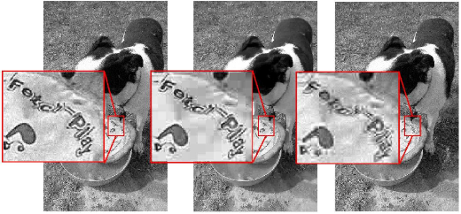
Figure 9: Close-up visual comparison of OMP and GHT-ADMM for sparse image denoising. (left) Noisy image with $\sigma=10$. OMP (right) uses a per patch budget of $s=10$ nonzeros while GHT-ADMM (middle) is given the equivalent global budget of $S=10P$.

4 Conclusions

In this work we have described two hard thresholding algorithms for approximately solving the joint sparse representation problem in (7). Both are penalty method approaches based on the notion of variable splitting, with the former being an instance of the Quadratic Penalty Method. While the latter, a heuristic adaptation of the popular ADMM framework, is not provably convergent it nonetheless consistently outperforms most of the popular algorithms for sparse representation and recovery in our extensive experiments on synthetic and natural image data. These experiments show that our algorithms distribute a global budget of nonzero coefficients much more effectively than naive patch-wise methods that use fixed local budgets. Additionally, both proposed algorithms are highly scalable making them attractive for researchers working on sparse recovery problems in signal and image processing. While we have presented experimental results for sparse image representation and denoising, the approaches discussed in this paper for solving (7) can be applied to a number of further image processing tasks such as image inpainting, deblurring, and super-resolution.

5 Acknowledgements

This work is supported in part by the GK-12 Reach For the Stars program through the National Science Foundation grant DGE-0948017, and the Department of Energy grant DE-NA0000457.

References

- [1] Y. C. Pati, R. Rezaiifar, P. Krishnaprasad, Orthogonal matching pursuit: Recursive function approximation with applications to wavelet decomposition, in: Signals, Systems and Computers, 1993. 1993 Conference Record of The Twenty-Seventh Asilomar Conference on, IEEE, 1993, pp. 40–44.
- [2] J. A. Tropp, A. C. Gilbert, Signal recovery from random measurements via orthogonal matching pursuit, Information Theory, IEEE Transactions on 53 (12) (2007) 4655–4666.
- [3] A. Beck, M. Teboulle, A fast iterative shrinkage-thresholding algorithm for linear inverse problems, SIAM Journal on Imaging Sciences 2 (1) (2009) 183–202.
- [4] T. Blumensath, Accelerated iterative hard thresholding, Signal Processing 92 (3) (2012) 752–756.
- [5] J. A. Tropp, A. C. Gilbert, M. J. Strauss, Algorithms for simultaneous sparse approximation. part i: Greedy pursuit, Signal Processing 86 (3) (2006) 572–588.
- [6] P. L. Combettes, V. R. Wajs, Signal recovery by proximal forward-backward splitting, Multiscale Modeling & Simulation 4 (4) (2005) 1168–1200.
- [7] E. Candes, J. Romberg, T. Tao, Robust uncertainty principles: Exact signal reconstruction from highly incomplete frequency information, IEEE Transactions on Information Theory 52 (2006) 489–509.
- [8] D. Donoho, Compressed sensing, IEEE Transactions on Information Theory 52 (2006) 1289–1306.
- [9] T. Blumensath, M. E. Davies, Normalized iterative hard thresholding: Guaranteed stability and performance, Selected Topics in Signal Processing, IEEE Journal of 4 (2) (2010) 298–309.
- [10] R. Garg, R. Khandekar, Gradient descent with sparsification: an iterative algorithm for sparse recovery with restricted isometry property, in: Proceedings of the 26th Annual International Conference on Machine Learning, ACM, 2009, pp. 337–344.
- [11] T. Blumensath, M. E. Davies, Iterative hard thresholding for compressed sensing, Applied and Computational Harmonic Analysis 27 (3) (2009) 265–274.
- [12] E. Candes, T. Tao, Decoding by linear programming, IEEE Transactions on Information Theory 51 (2005) 4203–4215.
- [13] P. Jain, R. Meka, I. S. Dhillon, Guaranteed rank minimization via singular value projection, in: Advances in Neural Information Processing Systems, 2010, pp. 937–945.
- [14] R. Meka, P. Jain, I. S. Dhillon, Guaranteed rank minimization via singular value projection, arXiv preprint arXiv:0909.5457.
- [15] M. Elad, M. Aharon, Image denoising via sparse and redundant representations over learned dictionaries, Image Processing, IEEE Transactions on 15 (12) (2006) 3736–3745.
- [16] M. Elad, M. Figueiredo, Y. Ma, On the role of sparse and redundant representations in image processing, Proceedings of the IEEE 98 (2010) 972–982.
- [17] J. Yang, J. Wright, T. S. Huang, Y. Ma, Image super-resolution via sparse representation, Image Processing, IEEE Transactions on 19 (11) (2010) 2861–2873.
- [18] E. Candes, C. Fernandez-Granda, Towards a mathematical theory of super-resolution, Communications on Pure and Applied Mathematics 67 (2014) 906–956.
- [19] B. A. Olshausen, D. J. Field, Sparse coding with an overcomplete basis set: A strategy employed by v1?, Vision research 37 (23) (1997) 3311–3325.
- [20] J. Nocedal, S. J. Wright, Penalty and Augmented Lagrangian Methods, Springer, 2006.
- [21] S. Boyd, N. Parikh, E. Chu, B. Peleato, J. Eckstein, Distributed optimization and statistical learning via the alternating direction method of multipliers, Foundations and Trends® in Machine Learning 3 (1) (2011) 1–122.
- [22] T. Goldstein, S. Osher, The split bregman method for l1-regularized problems, SIAM Journal on Imaging Sciences 2 (2) (2009) 323–343.
- [23] Y. Zhang, An alternating direction algorithm for nonnegative matrix factorization, preprint.
- [24] Y. Xu, W. Yin, Z. Wen, Y. Zhang, An alternating direction algorithm for matrix completion with nonnegative factors, Frontiers of Mathematics in China 7 (2) (2012) 365–384.
- [25] M. Hong, Z.-Q. Luo, M. Razaviyayn, Convergence analysis of alternating direction method of multipliers for a family of nonconvex problems, arXiv preprint arXiv:1410.1390.
- [26] S. Magnússon, P. C. Weeraddana, M. G. Rabbat, C. Fischione, On the convergence of alternating direction lagrangian methods for nonconvex structured optimization problems, arXiv preprint arXiv:1409.8033.
- [27] J. Watt, R. Borhani, A. Katsaggelos, A fast, effective, and scalable algorithm for symmetric nonnegative matrix factorization, NU Technical Report.
- [28] S. Barman, X. Liu, S. Draper, B. Recht, Decomposition methods for large scale lp decoding, in: Communication, Control, and Computing (Allerton), 2011 49th Annual Allerton Conference on, IEEE, 2011, pp. 253–260.
- [29] N. Derbinsky, J. Bento, V. Elser, J. S. Yedidia, An improved three-weight message-passing algorithm, arXiv preprint arXiv:1305.1961.
- [30] Q. Fu, H. W. A. Banerjee, Bethe-admm for tree decomposition based parallel map inference, in: Conference on Uncertainty in Artificial Intelligence (UAI), 2013.
- [31] P. Q. You, Seungil, A non-convex alternating direction method of multipliers heuristic for optimal power flow., IEEE SmartGridComm (to appear).
- [32] C. A. R. Hoare, Algorithm 65: find, Communications of the ACM 4 (7) (1961) 321–322.
- [33] R. W. Floyd, R. L. Rivest, Algorithm 489: the algorithm select for finding the i th smallest of n elements [m1], Communications of the ACM 18 (3) (1975) 173.
- [34] C. Martınez, Partial quicksort, in: Proc. 6th ACMSIAM Workshop on Algorithm Engineering and Experiments and 1st ACM-SIAM Workshop on Analytic Algorithmics and Combinatorics, 2004, pp. 224–228.
- [35] D. L. Donoho, V. C. Stodden, Y. Tsaig, About sparselab.
- [36] D. Needell, J. A. Tropp, Cosamp: Iterative signal recovery from incomplete and inaccurate samples, Applied and Computational Harmonic Analysis 26 (3) (2009) 301–321.
- [37] M. Elad, Sparse and redundant representations: from theory to applications in signal and image processing, Springer, 2010.
- [38] A. Hyvarinen, J. Hurri, P. O. Hoyer, Natural image statistics.