Multi-shot ASP solving with Clingo

Abstract

We introduce a new flexible paradigm of grounding and solving in Answer Set Programming (ASP), which we refer to as multi-shot ASP solving, and present its implementation in the ASP system clingo.

Multi-shot ASP solving features grounding and solving processes that deal with continuously changing logic programs. In doing so, they remain operative and accommodate changes in a seamless way. For instance, such processes allow for advanced forms of search, as in optimization or theory solving, or interaction with an environment, as in robotics or query-answering. Common to them is that the problem specification evolves during the reasoning process, either because data or constraints are added, deleted, or replaced. This evolutionary aspect adds another dimension to ASP since it brings about state changing operations. We address this issue by providing an operational semantics that characterizes grounding and solving processes in multi-shot ASP solving. This characterization provides a semantic account of grounder and solver states along with the operations manipulating them.

The operative nature of multi-shot solving avoids redundancies in relaunching grounder and solver programs and benefits from the solver’s learning capacities. clingo accomplishes this by complementing ASP’s declarative input language with control capacities. On the declarative side, a new directive allows for structuring logic programs into named and parameterizable subprograms. The grounding and integration of these subprograms into the solving process is completely modular and fully controllable from the procedural side. To this end, clingo offers a new application programming interface that is conveniently accessible via scripting languages. By strictly separating logic and control, clingo also abolishes the need for dedicated systems for incremental and reactive reasoning, like iclingo and oclingo, respectively, and its flexibility goes well beyond the advanced yet still rigid solving processes of the latter.

Under consideration for publication in Theory and Practice of Logic Programming (TPLP)

1 Introduction

Standard Answer Set Programming (ASP; [Baral (2003)]) follows a one-shot process in computing stable models of logic programs. This view is best reflected by the input/output behavior of monolithic ASP systems like dlv [Leone et al. (2006)] and (original) clingo [Gebser et al. (2011)] that take a logic program and output its stable models. Internally, however, both follow a fixed two-step process. First, a grounder generates a (finite) propositional representation of the input program. Then, a solver computes the stable models of the propositional program. This rigid process stays unchanged when grounding and solving with separate systems. In fact, up to series 3, clingo was a mere combination of the grounder gringo and the solver clasp. Although more elaborate reasoning processes are performed by the extended systems iclingo [Gebser et al. (2008)] and oclingo [Gebser et al. (2011)] for incremental and reactive reasoning, respectively, they also follow a pre-defined control loop evading any user control. Beyond this, however, there is substantial need for specifying flexible reasoning processes, for instance, when it comes to interactions with an environment (as in assisted living, robotics, or with users), advanced search (as in multi-objective optimization, planning, theory solving, or heuristic search), or recurrent query answering (as in hardware analysis and testing or stream processing). Common to all these advanced forms of reasoning is that the problem specification evolves during the respective reasoning processes, either because data or constraints are added, deleted, or replaced.

For mastering such complex reasoning processes, we propose the paradigm of multi-shot ASP solving in order to deal with continuously changing logic programs. In contrast to the traditional single-shot approach, where an ASP system takes a logic program, computes its answer sets, and exits, the idea is to consider evolving grounding and solving processes. Such processes lead to operative ASP systems that possess an internal state that can be manipulated by certain operations. Such operations allow for adding, grounding, and solving logic programs as well as setting truth values of (external) atoms. The latter does not only provide a simple means for incorporating external input but also for enabling or disabling parts of the current logic program. These functionalities allow for dealing with changing logic programs in a seamless way. To capture multi-shot solving processes, we introduce an operational semantics centered upon a formal definition of an ASP system state along with its (state changing) operations. Such a state reflects the relevant information gathered in the system’s grounder and solver components. This includes (i) a collection of non-ground logic programs subject to grounding, (ii) the ground logic programs currently held by the solver, (iii) and a truth assignment of externally defined atoms. Changing such a state brings about several challenges absent in the single-shot case, among them, contextual grounding and logic program composition.

Given that the theoretical foundations of multi-shot solving are a means to an end, we interleave their presentation with the corresponding features of ASP system clingo. This new generation of clingo offers novel high-level constructs for realizing multi-shot ASP solving. This is achieved within a single ASP grounding and solving process that avoids redundancies otherwise caused by relaunching grounder and solver programs and benefits from the learning capacities of modern ASP solvers. To this end, clingo complements ASP’s declarative input language by manifold control capacities. The latter are provided by an imperative application programming interface (API) implemented in C. Corresponding bindings for Python and Lua are available and can also be embedded into clingo’s input language (via the #script directive). On the declarative side, clingo offers a new directive #program that allows for structuring logic programs into named and parametrizable subprograms. The grounding and integration of these subprograms into the solving process is completely modular and fully controllable from the procedural side. For exercising control, the latter benefits from a dedicated library furnished by clingo’s API, which does not only expose grounding and solving functions but moreover allows for continuously assembling the solver’s program. This can be done in combination with externally controllable atoms that allow for enabling or disabling rules. Such atoms are declared by the #external directive. Hence, by strictly separating logic and control, clingo abolishes the need for special-purpose systems for incremental and reactive reasoning, like iclingo and oclingo, respectively, and its flexibility goes well beyond the advanced yet still rigid grounding and solving processes of such systems. In fact, clingo’s multi-shot solving capabilities rather enable users to engineer novel forms of reasoning, as we demonstrate by four case studies.

The rest of the paper is organized as follows. Section 2 provides a brief account of formal preliminaries. Section 3 gives an informal overview on the new features of clingo in order to pave the way for their formal underpinnings presented in Section 4. There, we lay the formal foundations of multi-shot solving and present its aforementioned operational semantics. In Section 5, we illustrate the power of multi-shot ASP solving in several use cases and highlight some features of interest. We use Python throughout the paper to illustrate the multi-shot functionalities of clingo’s API. Further API-related aspects are described in Section 6. Section 7 gives an empirical analysis of some selected features of multi-shot solving with clingo. Finally, we relate our approach to the literature in Section 8 before we conclude in Section 9.

2 Formal preliminaries

A (normal) rule $r$ is an expression of the form

$$a_{0}\leftarrow a_{1},\dots,a_{m},{\sim}{a_{m+1}},\dots,{\sim}{a_{n}},$$

where $a_{i}$, for $0\leq m\leq n$, is an atom of the form $p(t_{1},\dots,t_{k})$, $p$ is a predicate symbol of arity $k$, also written as $p/k$, and $t_{1},\dots,t_{k}$ are terms, built from constants, variables, and functions. Letting $h(r)=a_{0}$, $B(r)=\{a_{1},\dots,a_{m},{\sim}{a_{m+1}},\dots,{\sim}{a_{n}}\}$, $B(r)^{+}=\{a_{1},\dots,a_{m}\}$, and $B(r)^{-}=\{a_{m+1},\dots,a_{n}\}$, we also denote $r$ by $h(r)\leftarrow B(r)$. A rule is called fact, whenever $B(r)=\emptyset$. A (normal) logic program $P$ is a set (or list) of rules (depending on whether the order of rules matters or not). We write $H(P)=\{h(r)\mid r\in P\}$ and $A(P)=H(P)\cup\bigcup_{r\in P}(B(r)^{+}\cup B(r)^{-})$ to denote the set of all head atoms and atoms occurring in $P$, respectively. A term, atom, rule, or program is ground if it does not contain variables.

We denote the set of all ground terms constructible from constants (including all integers) and function symbols by $\mathcal{T}\!$, and let $\mathcal{C}$ stand for the subset of symbolic (i.e. non-integer) constants. The ground instance of $P$, denoted by $\mathit{grd}(P)$, is the set of all ground rules constructible from rules $r\in P$ by substituting every variable in $r$ with some element of $\mathcal{T}$. We associate $P$ with its positive atom dependency graph

$$G(P)=(A(\mathit{grd}(P)),\{(a_{0},a)\mid r\in\mathit{grd}(P),h(r)=a_{0},a\in B(r)^{+}\})$$

and call a maximal non-empty subset of $A(\mathit{grd}(P))$ inducing a strongly connected subgraph of $G(P)$ a strongly connected component of $P$.

A set $X$ of ground atoms is a model of $P$, if $h(r)\in X$, $B(r)^{+}\nsubseteq X$, or $B(r)^{-}\cap X\neq\emptyset$ holds for every $r\in\mathit{grd}(P)$. Moreover, $X$ is a stable model of $P$ [Gelfond and Lifschitz (1988)], if $X$ is a $\subseteq$-minimal model of $\{h(r)\leftarrow B(r)^{+}\mid r\in\mathit{grd}(P),\linebreak[1]B(r)^{-}\cap X=\nolinebreak\emptyset\}$.

Following ?), a module $\mathbb{P}$ is a triple $(P,I,O)$ consisting of a ground logic program $P$ along with sets $I$ and $O$ of ground input and output atoms such that

1. $I\cap\nolinebreak O=\nolinebreak\emptyset$,

2. $A(P)\subseteq I\cup O$, and

3. $H(P)\subseteq O$.

We also denote the constituents of $\mathbb{P}=(P,I,O)$ by $P(\mathbb{P})=\nolinebreak P$, $I(\mathbb{P})=\nolinebreak I$, and $O(\mathbb{P})=\nolinebreak O$. A set $X$ of ground atoms is a stable model of a module $\mathbb{P}$, if $X$ is a (standard) stable model of $P(\mathbb{P})\cup\{{a\leftarrow}\mid a\in I(\mathbb{P})\cap X\}$.

Two modules $\mathbb{P}_{1}$ and $\mathbb{P}_{2}$ are compositional, if

1. $O(\mathbb{P}_{1})\cap O(\mathbb{P}_{2})=\emptyset$ and

2. $O(\mathbb{P}_{1})\cap C=\emptyset$ or $O(\mathbb{P}_{2})\cap C=\emptyset$
   for every strongly connected component $C$ of $P(\mathbb{P}_{1})\cup P(\mathbb{P}_{2})$.

In other words, all rules defining an atom must belong to the same module. And any positive recursion is within modules; no positive recursion is allowed among modules.

Provided that $\mathbb{P}_{1}$ and $\mathbb{P}_{2}$ are compositional, their join is defined as the module

$$\mathbb{P}_{1}\sqcup\mathbb{P}_{2}=(P(\mathbb{P}_{1})\cup P(\mathbb{P}_{2}),\linebreak[1](I(\mathbb{P}_{1})\setminus O(\mathbb{P}_{2}))\cup(I(\mathbb{P}_{2})\setminus O(\mathbb{P}_{1})),\linebreak[1]O(\mathbb{P}_{1})\cup O(\mathbb{P}_{2}))\ .$$

The module theorem [Oikarinen and Janhunen (2006)] shows that a set $X$ of ground atoms is a stable model of $\mathbb{P}_{1}\sqcup\mathbb{P}_{2}$ iff $X=X_{1}\cup X_{2}$ for stable models $X_{1}$ and $X_{2}$ of $\mathbb{P}_{1}$ and $\mathbb{P}_{2}$, respectively, such that $X_{1}\cap(I(\mathbb{P}_{2})\cup O(\mathbb{P}_{2}))=X_{2}\cap(I(\mathbb{P}_{1})\cup O(\mathbb{P}_{1}))$. For example, the modules $\mathbb{P}_{1}=(\{a\leftarrow{\sim}{c};\ c\leftarrow{\sim}{b}\},\{b\},\{a,c\})$ and $\mathbb{P}_{2}=(\{b\leftarrow a\},\{a\},\{b\})$ are compositional, and combining their stable models, $\{a,b\}$ and $\{c\}$ for $\mathbb{P}_{1}$ as well as $\{a,b\}$ and $\emptyset$ for $\mathbb{P}_{2}$, yields the stable models $\{a,b\}$ and $\{c\}$ of $\mathbb{P}_{1}\sqcup\mathbb{P}_{2}=(P(\mathbb{P}_{1})\cup P(\mathbb{P}_{2}),\emptyset,\{a,b,c\})$. Unlike that, $\mathbb{P}_{1}^{\prime}=(\{a\leftarrow b;\ c\leftarrow{\sim}{a}\},\{b\},\{a,c\})$ and $\mathbb{P}_{2}$ are not compositional because the strongly connected component $\{a,b\}$ of $P(\mathbb{P}_{1}^{\prime})\cup P(\mathbb{P}_{2})$ includes $a\in O(\mathbb{P}_{1}^{\prime})$ and $b\in O(\mathbb{P}_{2})$. Moreover, $\{a,b\}$ is a stable model of $\mathbb{P}_{1}^{\prime}$ and $\mathbb{P}_{2}$, but not of $P(\mathbb{P}_{1}^{\prime})\cup P(\mathbb{P}_{2})$.

An assignment $v$ over a set $A$ of ground atoms is a function $v:A\rightarrow\{t,f,u\}$ whose range consists of truth values, standing for true, false, and undefined. Given an assignment $v$, we define the sets $V^{x}=\{a\in A\mid v(a)=x\}$ for $x\in\{t,f,u\}$. In what follows, we represent partial assignments like $v$ either by $(V^{t},V^{f})$ or $(V^{t},V^{u})$ by leaving the respective variables with default values implicit.

Finally, we use typewriter font and symbols :- and not instead of $\leftarrow$ and $\sim$, respectively, whenever we deal with source code accepted by clingo. In such a case, we also make use of extended language constructs like integrity or cardinality constraints, all of which can be reduced to normal logic programs, as detailed in the literature (cf. [Simons et al. (2002)]).

3 Multi-shot solving with clingo at a glance

Let us begin with an informal overview of the central features and corresponding language constructs of clingo’s multi-shot solving capacities.

A key feature, distinguishing clingo from its predecessors, is the possibility to structure (non-ground) input rules into subprograms. To this end, a program can be partitioned into several subprograms by means of the directive #program; it comes with a name and an optional list of parameters. Once given in the input, the directive gathers all rules up to the next such directive (or the end of file) within a subprogram identified by the supplied name and parameter list. As an example, two subprograms base and acid(k) can be specified as follows:

⬇

1a(1).

2#program acid(k).

3b(k).

4c(X,k) :- a(X).

5#program base.

6a(2).

Listing 1: Logic program with #program declarations

Note that base is a dedicated subprogram (with an empty parameter list): in addition to the rules in its scope, it gathers all rules not preceded by any #program directive. Hence, in the above example, the base subprogram includes the facts a(1) and a(2), although, only the latter is in the actual scope of the directive in Line 5. Without further control instructions (see below), clingo grounds and solves the base subprogram only, essentially, yielding the standard behavior of ASP systems. The processing of other subprograms such as acid(k) is subject to explicitly given control instructions.

For such customized control over grounding and solving, a main routine (taking a control object representing the state of clingo as argument, here prg) can be supplied. For illustration, let us consider two Python main routines:
       ⬇ 7#script(python) 8def main(prg): 9 prg.ground([("base",[])]) 10 prg.solve() 11#end. ⬇ 7#script(python) 8def main(prg): 9 prg.ground([("acid",[42])]) 10 prg.solve() 11#end.
While the control program on the left matches the default behavior of clingo, the one on the right ignores all rules in the base program but rather contains a ground instruction for acid(k) in Line 8, where the parameter k is to be instantiated with the term 42. Accordingly, the schematic fact b(k) is turned into b(42), no ground rule is obtained from ‘c(X,k) :- a(X)’ due to lacking instances of a(X), and the solve command in Line 10 yields a stable model consisting of b(42) only. Note that ground instructions apply to the subprograms given as arguments, while solve triggers reasoning w.r.t. all accumulated ground rules.

In order to accomplish more elaborate reasoning processes, like those of iclingo and oclingo or other customized ones, it is indispensable to activate or deactivate ground rules on demand. For instance, former initial or goal state conditions need to be relaxed or completely replaced when modifying a planning problem, e.g., by extending its horizon. While the predecessors of clingo relied on the #volatile directive to provide a rigid mechanism for the expiration of transient rules, clingo captures the respective functionalities and customizations thereof in terms of the #external directive. The latter goes back to lparse [Syrjänen (2001)] and was also supported by clingo’s predecessors to exempt (input) atoms from simplifications (and fixing them to false). As detailed in the following, the #external directive of clingo provides a generalization that, in particular, allows for a flexible handling of yet undefined atoms.

For continuously assembling ground rules evolving at different stages of a reasoning process, #external directives declare atoms that may still be defined by rules added later on. In terms of module theory, such atoms correspond to inputs, which (unlike undefined output atoms) must not be simplified. For declaring input atoms, clingo supports schematic #external directives that are instantiated along with the rules of their respective subprograms. To this end, a directive like

⬇

#external p(X,Y) : q(X,Z), r(Z,Y).

is treated similar to a rule ‘p(X,Y) :- q(X,Z), r(Z,Y)’ during grounding. However, the head atoms of the resulting ground instances are merely collected as inputs, whereas the ground rules as such are discarded.

Once grounded, the truth value of external atoms can be changed via the clingo API (until the atoms becomes defined by corresponding rules). By default, the initial truth value of external atoms is set to false. For example, with clingo’s Python API, assign_external(self,p(a,b),True) can be used to set the truth value of the external atom p(a,b) to true. Among others, this can be used to activate and deactivate rules in logic programs. For instance, the integrity constraint ‘:- q(a,c), r(c,b), p(a,b)’ is ineffective whenever p(a,b) is false.

4 Multi-shot solving

Having set the practical stage in the previous section, let us now turn to posing the formal foundations of multi-shot ASP solving. We begin with a characterization of grounding subprograms with external directives in the context of previously grounded subprograms. This provides us with a formal account of the interplay of ground routines with #program and #external directives. Next, we show how module theory can be used for characterizing the composition of ground subprograms during multi-shot solving. This gives us a precise idea on the successive logic programs contained in the ASP solver at each invocation of solve. Finally, all this culminates in an operational semantics for multi-shot solving in terms of state-changing operations.

The concepts introduced in this section are mainly illustrated by succinct, technical examples. More illustration is provided in the next section discussing several use cases in detail.

4.1 Parameterizable subprograms

A program declaration is of form

$$\texttt{\#program }n(p_{1},\dots,p_{k})$$ (1)

where $n,p_{1},\dots,p_{k}$ are symbolic constants. We call $n$ the name of the declaration and $p_{1},\dots,p_{k}$ its parameters. For simplicity, we suppose that different occurrences of program declarations with the same name also share the same parameters (although this is not required by clingo). In this way, each name is associated with a unique parameter specification.

The scope of a program declaration in a list of rules and declarations consists of the set of all rules and non-program declarations following the directive up to the next program declaration or the end of the list. In Listing 1, the scope of the declaration in Line 2 consists of b(k) and ‘c(X,k) :- a(X)’, while that in Line 5 contains a(2). Given a list $R$ of (non-ground) rules and declarations along with a non-integer constant $n$, we define $R(n)$ as the set of all (non-ground) rules and (non-program) declarations in the scope of all occurrences of program declarations with name $n$. We often refer to $R(n)$ as a subprogram of $R$. All rules and non-program declarations outside the scope of any (explicit) program declaration are thought of being implicitly preceded by a ‘#program base’ declaration. Hence, if $R$ consists of Line 1–6 above, we get $R(\texttt{base})=\{a(1)\leftarrow{},a(2)\leftarrow{}\}$ and $R(\texttt{acid})=\{b(k)\leftarrow{},c(X,k)\leftarrow a(X)\}$. Each such list $R$ induces a collection $(R(c))_{c\in\mathcal{C}}$ of (non-disjoint) subprograms (most of which are empty). For example, all subprograms obtained from Line 1–6 are empty, except for base and acid.

Given a name $n$ with associated parameters $p_{1},\dots,p_{k}$, the instantiation of subprogram $R(n)$ with terms $t_{1},\dots,t_{k}$ results in the set $R(n)[p_{1}/t_{1},\dots,p_{k}/t_{k}]$, obtained by replacing in $R(n)$ each occurrence of $p_{i}$ by $t_{i}$ for $1\leq i\leq k$. For instance, $R(\texttt{acid})[\mathtt{k}/\mathtt{42}]$ consists of b(42) and ‘c(X,42) :- a(X)’.

4.2 Contextual grounding

The definition of a program’s ground instance $\mathit{grd}(P)$ depends on $P$ and its underlying set of terms. For instance, grounding accordingly program $R(\texttt{base})\cup R(\texttt{acid})[k/42]$ yields

$$\{a(1)\leftarrow{},a(2)\leftarrow{}\}\cup\{b(42)\leftarrow{}\}\cup\left\{\begin{array}[]{rcl}c(1,42)&\leftarrow&a(1),\\ c(2,42)&\leftarrow&a(2),\\ c(42,42)&\leftarrow&a(42)\end{array}\right\}$$ (5)

In practice, however, rules are grounded relative to a set of atoms, which we refer to as an atom base. In our example, this avoids the generation of the irrelevant rule ‘$c(42,42)\leftarrow a(42)$’. To see this, note that the relevance of instances of ‘$c(X,42)\leftarrow a(X)$’ depends upon the available ground atoms of predicate $a/1$. Now, grounding first $R$(base) establishes — in addition to $\mathit{grd}(R(\texttt{base}))$ — the atom base $\{a(1),a(2)\}$. Grounding then $R(\texttt{acid})[k/42]$ relative to this atom base, yields

$$\{b(42)\leftarrow{}\}\cup\left\{\begin{array}[]{rcl}c(1,42)&\leftarrow&a(1),\\ c(2,42)&\leftarrow&a(2)\end{array}\right\}$$ (8)

because only rule instances are created if their positive body literals either belong to the atom base or are derivable through other rules instances. Hence, rule $c(42,42)\leftarrow a(42)$ is dropped. This is made precise in view of our purpose in the following definition.

Given a set $R$ of (non-ground) rules and two sets $C,D$ of ground atoms, we define an instantiation of $R$ relative to atom base $C$ as a ground program $\mathit{grd}_{C}(R)$ over atom base $D$ subject to the following conditions:

$$D =C\cup H(\mathit{grd}_{C}(R))$$ (9)

$$\mathit{grd}_{C}(R) {}\subseteq\{h(r)\leftarrow B(r)^{+}\cup\{{\sim}{a}\mid{}\begin{array}[t]{@{}r@{}l@{}}a\in{}&B(r)^{-}\cap D\}\mid{}\\ r\in{}&\mathit{grd}(R),B(r)^{+}\cup\{h(r)\}\subseteq D\}\end{array}$$ (12)

$$\mathit{grd}_{C}(R) {}\cup Q\text{ and }\mathit{grd}(R)\cup Q\text{ have the same stable models}$$ (13)

where $Q=\{{\{a\}\leftarrow}{}\mid a\in C\setminus H(\mathit{grd}(R))\}$.

Atom base $D$ gives the extension of $C$ obtained by grounding $R$ relative to $C$. To this end, Condition (9) limits $D$ to atoms either belonging to $C$ or emerging as heads of rules in $\mathit{grd}_{C}(R)$, while Condition (12) projects $\mathit{grd}(P)$ to $D$ by reducing its rules to those parts possibly relevant to stable models, as expressed in (13). The exact scope of the obtained atom base $D$ as well as $\mathit{grd}_{C}(R)$ are left open to account for potential simplifications during grounding. The correctness of the specific scope is warranted by Condition (13)

We capture the composition of ground programs below in Section 4.4 in terms of modules. To this end, note that the choices in $Q$ mimic the role of input atoms of modules. In fact, Condition (13) is equivalent to requiring that the modules $(\mathit{grd}_{C}(R),\linebreak[1]C\setminus H(\mathit{grd}(R)),\linebreak[1]H(\mathit{grd}(R)))$ and $(\mathit{grd}(R),\linebreak[1]C\setminus H(\mathit{grd}(R)),\linebreak[1]H(\mathit{grd}(R)))$ have the same stable models.

Resuming our example, we see that $\mathit{grd}_{\{a(1),a(2)\}}(R(\texttt{acid})[k/42])$ corresponds to the rules in (8). Together with $\mathit{grd}_{\emptyset}(R(\texttt{base}))$, the resulting program is equivalent to $\mathit{grd}(R(\texttt{base})\cup R(\texttt{acid})[k/42])$, viz. the rules in (5).

For further illustration, consider $R=\{a(X)\leftarrow f(X),e(X);\ b(X)\leftarrow f(X),{\sim}{e(X)}\}$ along with $C=\{f(1),f(2),e(1)\}$. Focusing on relevant (parts of) rule instances relative to $C$ leads to

$$\mathit{grd}_{C}(R)=\left\{\begin{array}[]{ll}a(1)\leftarrow f(1),e(1)&b(1)\leftarrow f(1),{\sim}{e(1)}\\ &b(2)\leftarrow f(2)\end{array}\right\}$$

over $D=C\cup\{a(1),b(1),b(2)\}$. In particular, note that an inapplicable rule instance including $e(2)$ is dropped, while ${\sim}{e(2)}$ is simplified away to thus obtain the last of the above ground rules.

Although $\mathit{grd}_{C}(R)$ reflects a potential simplification of the full ground program $\mathit{grd}(R)$, both can likewise be augmented with additional rules. Moreover, the restriction of the resulting atom base preserves equivalence. The next result makes this precise in terms of module theory.

Proposition 1

Let $R$ be a set of (non-ground) rules, let $\mathit{grd}_{C}(R)$ be an instantiation of $R$ relative to a set $C$ of ground atoms, and let $\mathbb{P}$ be a module.

If $\mathbb{P}$ and $(\mathit{grd}(R),\linebreak[1]C\setminus H(\mathit{grd}(R)),\linebreak[1]H(\mathit{grd}(R)))$ are compositional, then $\mathbb{P}$ and $(\mathit{grd}_{C}(R),\linebreak[1]C\setminus H(\mathit{grd}(R)),\linebreak[1]H(\mathit{grd}(R)))$ are compositional as well, where $\mathbb{P}\sqcup(\mathit{grd}(R),\linebreak[1]C\setminus H(\mathit{grd}(R)),\linebreak[1]H(\mathit{grd}(R)))$ and $\mathbb{P}\sqcup(\mathit{grd}_{C}(R),\linebreak[1]C\setminus H(\mathit{grd}(R)),\linebreak[1]H(\mathit{grd}(R)))$ have the same stable models.

Proof 4.1.

Assume that $\mathbb{P}$ and $(\mathit{grd}(R),\linebreak[1]C\setminus H(\mathit{grd}(R)),\linebreak[1]H(\mathit{grd}(R)))$ are compositional. By the construction of $\mathit{grd}_{C}(R)$ in (12), $G(\mathit{grd}_{C}(R))$ is a subgraph of $G(\mathit{grd}(R))$, which implies that $\mathbb{P}$ and $(\mathit{grd}_{C}(R),\linebreak[1]C\setminus H(\mathit{grd}(R)),\linebreak[1]H(\mathit{grd}(R)))$ are compositional as well. As $(\mathit{grd}(R),\linebreak[1]C\setminus H(\mathit{grd}(R)),\linebreak[1]H(\mathit{grd}(R)))$ and $(\mathit{grd}_{C}(R),\linebreak[1]C\setminus H(\mathit{grd}(R)),\linebreak[1]H(\mathit{grd}(R)))$ are equivalent by the condition in (13), the module theorem [Oikarinen and Janhunen (2006)] yields that $\mathbb{P}\sqcup(\mathit{grd}(R),\linebreak[1]C\setminus H(\mathit{grd}(R)),\linebreak[1]H(\mathit{grd}(R)))$ and $\mathbb{P}\sqcup(\mathit{grd}_{C}(R),\linebreak[1]C\setminus H(\mathit{grd}(R)),\linebreak[1]H(\mathit{grd}(R)))$ have the same stable models.

More illustration of contextual grounding is given throughout the following sections.

4.3 Extensible logic programs

We define a (non-ground) logic program $R$ as extensible, if it contains some (non-ground) external declaration of the form

$${\text{\leavevmode\lstinline{{\lst@@@set@language\lst@@@set@numbers\lst@@@set@frame\lst@@@set@rulecolor\lst@@@set@numbers\#{\@listingGroup{ltx_lst_identifier}{external}}}}}}~{}a:B$$ (14)

where $a$ is an atom and $B$ a rule body.

As an example, consider the extensible program in Listing 2.

⬇

1#external e(X) : f(X), X < 2.

2f(1..2).

3a(X) :- f(X), e(X).

4b(X) :- f(X), not e(X).

Listing 2: Extensible logic program

For grounding an external declaration as in (14), we treat it as a rule $a\leftarrow B,\varepsilon$ where $\varepsilon$ is a distinguished ground atom marking rules from #external declarations. Formally, given an extensible program $R$, we define the collection $Q$ of rules corresponding to #external declarations as follows.

$$Q {}=\{a\leftarrow B,\varepsilon\mid({\texttt{\#external}}~{}a:B)\in R\}$$

$$R^{\prime} {}=\{a\leftarrow B\in R\}$$

With these, the ground instantiation of an extensible logic program $R$ relative to an atom base $C$ is defined as a ground logic program $P$ associated with a set $E$ of ground atoms, where

$$P {}=\{r\in\mathit{grd}_{C\cup\{\varepsilon\}}(R^{\prime}\cup Q)\mid\varepsilon\notin B(r)\}$$ (15)

$$E {}=\{h(r)\mid r\in\mathit{grd}_{C\cup\{\varepsilon\}}(R^{\prime}\cup Q),\varepsilon\in B(r)\}$$ (16)

For simplicity, we refer to $P$ and $E$ as a logic program with externals, and we drop the reference to $R$ and $C$ whenever clear from the context. Note that after grounding, the special atom $\varepsilon$ appears neither in $P$ nor $E$. In fact, $P$ is a logic program over $C\cup E\cup H(P)$.

Given the set $E$ of externals, $P$ can alternatively be defined as $\mathit{grd}_{C\cup E}(R^{\prime})$.

Grounding the program in Listing 2 relative to an empty atom base yields the below program with a single external atom, viz. e(1):

⬇

1f(1). f(2).

2a(1) :- f(1), e(1).

3b(1) :- f(1), not e(1).

4b(2) :- f(2).

Note how externals influence the result of grounding. While occurrences of e(1) remain untouched, the atom e(2) is unavailable and thus set to false according to the condition in (12). In practice, even more simplifications are applied during grounding. For instance, in clingo, the established truth of f(1) and f(2) leads to their removal in the bodies in Line 2–4.

Logic programs with externals constitute a major building block of multi-shot solving. Hence, before addressing their composition within a more elaborate formal framework, let us provide some semantic underpinnings. The stable models of such programs are defined relative to a truth assignment on the external atoms. For a program $P$ with externals $E$, we define the set $I=E\setminus H(P)$ as input atoms of $P$. That is, input atoms are externals that are not overridden by rules in $P$. Then, given $P$ along with a partial assignment $V=(V^{t},V^{u})$ over $I$, we define the stable models of $P$ w.r.t. $V$ as the ones of $P\cup(\{{a\leftarrow{}}\mid a\in V^{t}\}\cup\{{\{a\}\leftarrow{}}\mid a\in V^{u}\})$ to capture the extension of $P$ with respect to a truth assignment to the input atoms in $I$. Note that the externals in $E$ remain implicit in the domain of $V$. For instance, the above program $P$ with externals ${E=\{\text{\leavevmode\lstinline{{\lst@@@set@language\lst@@@set@numbers\lst@@@set@frame\lst@@@set@rulecolor\lst@@@set@numbers{\@listingGroup{ltx_lst_identifier}{e}}(1)}}}}\!\}$ has a stable model including a(1) but excluding b(1) w.r.t. assignment $(\{\texttt{e(1)}\},\emptyset)$, and vice versa with $(\emptyset,\emptyset)$.

Further examples involving external atoms are given in Listings 3, 7, 10, 11, and 15 below.

4.4 Composing logic programs with externals

The assembly of (ground) subprograms can be characterized by means of module theory. Program states are captured by modules whose input and output atoms provide the respective atom base. Successive grounding instructions result in modules to be joined with the modules of the corresponding program states.

Given an atom base $C$, a (non-ground) extensible program $R$ yields the module

$${C}=(P,(C\cup E)\setminus H(P),H(P))$$ (17)

via the ground program $P$ with externals $E$ obtained by grounding $R$ relative to $C$. For example, grounding the extensible program in Listing 2 w.r.t. the empty atom base results in the module in (18).

$$\left(\left\{\begin{array}[]{l}f(1)\leftarrow{}\\ f(2)\leftarrow{}\\ a(1)\leftarrow f(1),e(1)\\ b(1)\leftarrow f(1),{\sim}{e(1)}\\ b(2)\leftarrow f(2)\end{array}\right\},\left\{e(1)\right\},\left\{\begin{array}[l]{l}f(1),f(2),{}\\ a(1),{}\\ b(1),b(2)\end{array}\right\}\right)$$ (18)

Given the induction of modules from extensible programs w.r.t. to atom bases in (17), we define successive program states in the following way.

The initial program state is given by the empty module $\mathbb{P}_{0}=(\emptyset,\emptyset,\emptyset)$.

The program state succeeding a module $\mathbb{P}_{i}$ is captured by the module

$$\mathbb{P}_{i+1}=\mathbb{P}_{i}\sqcup{I(\mathbb{P}_{i})\cup O(\mathbb{P}_{i})}$$ (19)

where ${I(\mathbb{P}_{i})\cup O(\mathbb{P}_{i})}$ gives the result of grounding an extensible program $R$ relative to the atom base $I(\mathbb{P}_{i})\cup O(\mathbb{P}_{i})$ as defined in (17). Note that $P({I(\mathbb{P}_{i})\cup O(\mathbb{P}_{i})})$ is a logic program over $I(\mathbb{P}_{i+1})\cup O(\mathbb{P}_{i+1})$ with externals $E$ such that

$$I(\mathbb{P}_{i+1})\cup O(\mathbb{P}_{i+1})\ =\ (I(\mathbb{P}_{i})\cup O(\mathbb{P}_{i}))\cup E\cup H(P({I(\mathbb{P}_{i})\cup O(\mathbb{P}_{i})}))).$$

This reflects the atom base of programs with externals discussed after equations (15) and (16). From a practical point of view, the modules $\mathbb{P}_{i}$ and $\mathbb{P}_{i+1}$ represent the program state of clingo before and after the $(i{+}1)$-st execution of a ground command in a main routine. And ${I(\mathbb{P}_{i})\cup O(\mathbb{P}_{i})}$ captures the result of the $(i{+}1)$-st ground command applied to an extensible program relative to the atom base provided by $\mathbb{P}_{i}$. Notably, the join leading to $\mathbb{P}_{i+1}$ can be undefined in case the constituent modules are non-compositional. At system level, compositionality is only partially checked. clingo, or more precisely clasp, respectively, issues an error message when atoms become redefined but no cycle check over modules is done.

Interestingly, input atoms induced by externals can also be used to incorporate future information. To see this, consider the following rules (extracted from Listing 10):

⬇

1#program s(i).

2#external a(i).

4{ q(i) }.

5a(i-1) :- q(i).

6a(i-1) :- a(i).

7 :- a(i), q(i).

These rules give rise to the module $\mathbb{S}_{i}(C)$ given as follows.

$$\left(\left\{\begin{array}[]{ccl}\{q(i)\}&\leftarrow&\\ a(i-1)&\leftarrow&q(i)\\ a(i-1)&\leftarrow&a(i)\\ &\leftarrow&a(i),q(i)\end{array}\right\},(C\cup\{a(i)\})\setminus\{a(i-1),q(i)\},\{a(i-1),q(i)\}\right)$$ (24)

We observe that the input atom $a(i)$ of $\mathbb{S}_{i}(C)$ is defined in $\mathbb{S}_{i+1}(C)$. Proceeding as in (19) by letting $\mathbb{R}$ be $\mathbb{S}$, each module $\mathbb{P}_{i}$ has a single input atom $a(i)$ and output atoms $\{a(0),\dots,a(i-1),q(1),\dots,q(i)\}$; it yields $i+1$ stable models, either the empty one or one of the form $\{a(0),\dots,a(j-1),q(j)\}$ for $1\leq j\leq i$. In the latter models, the truth of an atom like $a(0)$ relies on that of $q(j)$, occurring in a subsequently joined module whenever $j\geq 2$.

The next result provides a characterization of sequences of program states in terms of their constituent subprograms and their associated external atoms. The well-definedness of a sequence depends upon their compositionality, as defined in Section 2.

Proposition 4.2.

Let $(R_{i})_{i>0}$ be a sequence of (non-ground) extensible programs, and let $P_{i+1}$ be the ground program with externals $E_{i+1}$ obtained from $R_{i+1}$ and $I(\mathbb{P}_{i})\cup O(\mathbb{P}_{i})$ for $i\geq 0$, where $\mathbb{P}_{0}=(\emptyset,\emptyset,\emptyset)$ and $\mathbb{P}_{i+1}$ is defined as in (19), and $\mathbb{R}_{i+1}$ is defined as in (17) for $i\geq 0$.

If $\mathbb{P}_{i}$ and ${I(\mathbb{P}_{i})\cup O(\mathbb{P}_{i})}$ are compositional for some $j\geq 0$ and all $j>i\geq 0$, then

1. $P(\mathbb{P}_{j})=\bigcup_{i>0}^{j}P_{i}$

2. $\;I(\mathbb{P}_{j})=\bigcup_{i>0}^{j}E_{i}\setminus\bigcup_{i>0}^{j}H(P_{i})$

3. $O(\mathbb{P}_{j})=\bigcup_{i>0}^{j}H(P_{i})$

Proof 4.3.

For $\mathbb{P}_{0}=(\emptyset,\emptyset,\emptyset)$, we have that $P(\mathbb{P}_{0})=I(\mathbb{P}_{0})=O(\mathbb{P}_{0})=\emptyset$, and assume that $P(\mathbb{P}_{j})=\bigcup_{i>0}^{j}P_{i}$, $I(\mathbb{P}_{j})=\bigcup_{i>0}^{j}E_{i}\setminus\bigcup_{i>0}^{j}H(P_{i})$, and $O(\mathbb{P}_{j})=\bigcup_{i>0}^{j}H(P_{i})$ for some $j\geq 0$. According to (15)–(17) and (19), ${I(\mathbb{P}_{j})\cup O(\mathbb{P}_{j})}$ is the module $(P_{j+1},\linebreak[1](I(\mathbb{P}_{j})\cup O(\mathbb{P}_{j})\cup E_{j+1})\setminus H(P_{j+1}),\linebreak[1]H(P_{j+1}))$, where

$$\begin{array}[]{@{}l@{}l@{}}P_{j+1}={}&\{r\in\mathit{grd}_{I(\mathbb{P}_{j})\cup O(\mathbb{P}_{j})\cup\{\varepsilon\}}(\begin{array}[t]{@{}l@{}}\{a\leftarrow B\in R_{j+1}\}\cup{}\\ \{a\leftarrow B,\varepsilon\mid(\texttt{\#external}~{}a:B)\in R_{j+1}\})\mid\varepsilon\notin B(r)\}\end{array}\\ E_{j+1}={}&\{h(r)\mid r\in\mathit{grd}_{I(\mathbb{P}_{j})\cup O(\mathbb{P}_{j})\cup\{\varepsilon\}}(\begin{array}[t]{@{}l@{}}\{a\leftarrow B\in R_{j+1}\}\cup{}\\ \{a\leftarrow B,\varepsilon\mid(\texttt{\#external}~{}a:B)\in R_{j+1}\}),\varepsilon\in B(r)\}\end{array}\end{array}$$

Provided that $\mathbb{P}_{j}$ and ${I(\mathbb{P}_{j})\cup O(\mathbb{P}_{j})}$ are compositional, their join is defined as

$$\mathbb{P}_{j+1}=\left(\begin{array}[]{l}\bigcup_{i>0}^{j+1}P_{i},{}\\ \bigcup_{i>0}^{j}E_{i}\setminus\bigcup_{i>0}^{j+1}H(P_{i})\cup(\bigcup_{i>0}^{j+1}E_{i}\cup\bigcup_{i>0}^{j}H(P_{i}))\setminus\bigcup_{i>0}^{j+1}H(P_{i}),{}\\ \bigcup_{i>0}^{j+1}H(P_{i})\end{array}\right)$$

That is, $P(\mathbb{P}_{j+1})=\bigcup_{i>0}^{j+1}P_{i}$, $I(\mathbb{P}_{j+1})=\bigcup_{i>0}^{j+1}E_{i}\setminus\bigcup_{i>0}^{j+1}H(P_{i})$, and $O(\mathbb{P}_{j+1})=\bigcup_{i>0}^{j+1}H(P_{i})$.

The ground rules in $P({I(\mathbb{P}_{i})\cup O(\mathbb{P}_{i})})$ are obtained by grounding $R_{i+1}$ relative to the atom base $I(\mathbb{P}_{i})\cup O(\mathbb{P}_{i})$, viz. the previously gathered input and output atoms. Unlike this, the full ground program $\mathit{grd}(R_{i+1})$ takes all ground terms into account; this includes all integers. Thus, for example, grounding the extensible program in Listing 2 in full yields an infinite module:

$$\left(\left\{\begin{array}[]{l}f(1)\leftarrow{}\\ f(2)\leftarrow{}\\ a(1)\leftarrow f(1),e(1){}\\ b(1)\leftarrow f(1),{\sim}{e(1){}}\\ a(2)\leftarrow f(2),e(2){}\\ b(2)\leftarrow f(2),{\sim}{e(2){}}\\ a(3)\leftarrow f(3),e(3){}\\ b(3)\leftarrow f(3),{\sim}{e(3){}}\\ \dots\end{array}\right\},\left\{e(1)\right\},\left\{\begin{array}[l]{l}f(1),f(2),{}\\ a(1),a(2),a(3),\dots\\ b(1),b(2),b(3),\dots\end{array}\right\}\right)$$ (25)

Both this module and the one in (18) obtained by contextual grounding possess two stable models: $X_{1}=\{e(1),f(1),f(2),a(1),b(2)\}$ and $X_{2}=\{f(1),f(2),b(1),b(2)\}$. However, when joined with the module $(\{e(2)\leftarrow\},\emptyset,\{e(2)\})$, the stable models of (18) turn into $X_{1}\cup\{e(2)\}$ and $X_{2}\cup\{e(2)\}$, while (25) yields $X_{1}\setminus\{b(2)\}\cup\{e(2),a(2)\}$ and $X_{2}\setminus\{b(2)\}\cup\{e(2),a(2)\}$. This mismatch results from the fact that the atom $e(2)$ was removed from (18) when grounding relative to atom base $\{e(1)\}$. The subsequent definition of $e(2)$ in module $(\{e(2)\leftarrow\},\emptyset,\{e(2)\})$ is thus stripped of any logical relation to the rules in (18). Such differences can be eliminated by stipulating $H(\mathit{grd}(R_{j+1}))\cap\bigcup_{i>0}^{j}A(\mathit{grd}(R_{i}))\subseteq I(\mathbb{P}_{j})$ for a sequence $(R_{i})_{i>0}$ of extensible programs and all $j\geq 0$, where the program state $\mathbb{P}_{j}$ is obtained through contextual grounding. This condition rules out the join conducted in our example. But even so, full and contextual grounding would still be imbalanced. For example, the module in (18) can be joined with modules defining $a(3),b(3),\dots$, while doing the same with (25) violates compositionality. Not to mention that infinite ground programs as in (25) cannot be utilized in practice. This discussion shows the influence of contextual grounding on inputs, outputs, and resulting ground programs. Hence, some care has to be taken when writing interacting subprograms. Actually, apart from the ones in Section 5.2, all following modules obtained by grounding parametrized programs satisfy the above condition and have the same solutions no matter which form of grounding is used.

4.5 State-based characterization of multi-shot solving

For capturing multi-shot solving, we must account for sequences of system states, involving information about the programs kept within the grounder and the solver. To this end, we define a simple operational semantics based on system states and associated operations.

An ASP system state is a triple $(\boldsymbol{R},\mathbb{P},V)$ where

• $\boldsymbol{R}=\left(R_{c}\right)_{c\in\mathcal{C}}$ is a collection of extensible (non-ground) logic programs,

• $\mathbb{P}$ is a module,

• $V=(V^{t},V^{u})$ is a three-valued assignment over $I(\mathbb{P})$.

When solving with $\mathbb{P}$, the input atoms in $I(\mathbb{P})$ are taken to be false by default, that is, $V^{f}=I(\mathbb{P})\setminus(V^{t}\cup V^{u})$. This can still be altered by dedicated directives as illustrated below.

As informal examples for ASP system states, consider the ones obtained from the program in Listing 1 after separately grounding subprograms base and acid (while replacing k with 42), respectively:

$$((R(\texttt{base}),R(\texttt{acid})),(\{a(1)\leftarrow{},a(2)\leftarrow{}\},\emptyset,\{a(1),a(2)\}),(\emptyset,\emptyset))$$ (26)

$$((R(\texttt{base}),R(\texttt{acid})),(\{b(42)\leftarrow{}\},\emptyset,\{b(42)\}),(\emptyset,\emptyset))$$ (27)

Given that the program in Listing 1 has no external declarations, no truth values can be assigned. This is different in states obtained from the program in Listing 2. Grounding this yields the state

$$((R(\texttt{base})),\mathbb{R}_{b},(\emptyset,\emptyset))$$ (28)

where $\mathbb{R}_{b}$ is the module given in (18). Furthermore, we have set the external atom $e(1)$ to false. The way such states are obtained from non-ground logic programs is made precise next.

ASP system states can be created and modified by the following operations.

Function create partitions a program into subprograms.

$\mathit{create}(R):{}\mapsto(\boldsymbol{R},\mathbb{P},V)$

for a list $R$ of (non-ground) rules and declarations where

• $\boldsymbol{R}=\left(R(c)\right)_{c\in\mathcal{C}}$

• $\mathbb{P}=(\emptyset,\emptyset,\emptyset)$

• $V=(\emptyset,\emptyset)$

Each subprogram $R(c)$ gathers all rules and non-program directives in the scope of $c$.

The respective subprograms can be extended by function add with rules as well as external declarations.

$\mathit{add}(R):(\boldsymbol{R}_{1},\mathbb{P},V)\mapsto(\boldsymbol{R}_{2},\mathbb{P},V)$

for a list $R$ of (non-ground) rules and declarations where

• $\boldsymbol{R}_{1}=\left(R_{c}\right)_{c\in\mathcal{C}}$ and $\boldsymbol{R}_{2}=\left(R_{c}\cup R(c)\right)_{c\in\mathcal{C}}$

Obviously, we have $\mathit{add}(R)(\mathit{create}(\emptyset))=\mathit{create}(R)$. Note that add only affects non-ground subprograms and thus ignores compositionality issues since they appear on the ground level.

Function ground instantiates the designated subprograms in $\boldsymbol{R}$ and binds their parameters. The resulting ground programs along with their external atoms are then joined with the ones captured in the current state — provided that they are compositional.

$\mathit{ground}((n,\boldsymbol{t}_{n})_{n\in\mathcal{N}}):(\boldsymbol{R},\mathbb{P}_{1},V_{1})\mapsto(\boldsymbol{R},\mathbb{P}_{2},V_{2})$

for a collection $(n,\boldsymbol{t}_{n})_{n\in\mathcal{N}}$ of pairs of non-integer constants $\mathcal{N}\subseteq\mathcal{C}$ and term tuples $\boldsymbol{t}_{n}\in\mathcal{T}^{k_{n}}$ of arity $k_{n}$ where

• $\mathbb{P}_{2}=\mathbb{P}_{1}\sqcup{I(\mathbb{P}_{1})\cup O(\mathbb{P}_{1})}$
  and $I(\mathbb{P}_{1})$∪$O(\mathbb{P}_{1})$ is the module obtained as in (17) from

  • extensible program $\bigcup_{n\in\mathcal{N}}R_{n}[p_{1}/t_{1},\dots,p_{k_{n}}/t_{k_{n}}]$ where $\boldsymbol{t}_{n}=(t_{1},\dots,t_{k_{n}})$ and

  • atom base $I(\mathbb{P}_{1})\cup O(\mathbb{P}_{1})$

  for $\left(R_{c}\right)_{c\in\mathcal{C}}=\boldsymbol{R}$

• $V_{2}^{t}\,=\{a\in I(\mathbb{P}_{2})\mid V_{1}(a)=t\,\}$

• $V_{2}^{u}=\{a\in I(\mathbb{P}_{2})\mid V_{1}(a)=u\}$

A few more technical remarks are in order. First, note that a previous external status of an atom is eliminated once it becomes defined by a ground rule. This is accomplished by module composition, namely, the elimination of output atoms from input atoms. Second, note that jointly grounded subprograms are treated as a single logic program. In fact, while $\mathit{ground}((c,\boldsymbol{p}_{c}),(c,\boldsymbol{p}_{c}))(s)$ and $\mathit{ground}((c,\boldsymbol{p}_{c}))(s)$ yield the same result, $\mathit{ground}((c,\boldsymbol{p}_{c}))(\mathit{ground}((c,\boldsymbol{p}_{c}))(s))$ leads to two non-compositional modules whenever normal rules are contained in $R_{c}$. Finally, note that new inputs stemming from just added external declarations are set to false in view of $V_{2}^{f}=I(\mathbb{P}_{2})\setminus(V_{2}^{t}\cup V_{2}^{u})$.

The above functionality lets us now formally characterize the states in (26) and (27). By abbreviating the logic program in Listing 1 with $R$, the system state in (26) results from $\mathit{ground}((\texttt{base},()))(\mathit{create}(R))$, while $\mathit{ground}((\texttt{acid},(\texttt{42})))(\mathit{create}(R))$ yields (27). Moreover, observe the difference between grounding subprogram acid before base and vice versa. While the ground program comprised in

$$\mathit{ground}((\texttt{base},()))(\mathit{ground}((\texttt{acid},(\texttt{42})))(\mathit{create}(R)))$$

only consists of the facts $\{b(42)\leftarrow{},a(1)\leftarrow{},a(2)\leftarrow{}\}$, the one contained in

$$\mathit{ground}((\texttt{acid},(\texttt{42})))(\mathit{ground}((\texttt{base},()))(\mathit{create}(R)))$$

includes additionally the rules $\{c(1,42)\leftarrow a(1);\ c(2,42)\leftarrow a(2)\}$. This difference is due to contextual grounding (cf. Section 4.2). While in the first case rule $c(X,42)\leftarrow a(X)$ is grounded w.r.t. atom base $\{b(42)\}$, it is grounded relative to $\{a(1),a(2),b(42)\}$ in the second case. Such effects are obviously avoided when jointly grounding both subprograms, as in

$$\mathit{ground}((\texttt{base},()),(\texttt{acid},(\texttt{42})))(\mathit{create}(R))\ .$$

The next function allows us to change the truth assignment of input atoms.

$\mathit{assignExternal}(a,v):(\boldsymbol{R},\mathbb{P},V_{1})\mapsto(\boldsymbol{R},\mathbb{P},V_{2})$

for a ground atom $a$ and $v\in\{t,u,f\}$ where

• if $v=t$

  • $V_{2}^{t}\,=V_{1}^{t}\cup\{a\}$ if $a\in I(\mathbb{P})$, and $V_{2}^{t}=V_{1}^{t}$ otherwise

  • $V_{2}^{u}=V_{1}^{u}\setminus\{a\}$

• if $v=u$

  • $V_{2}^{t}\,=V_{1}^{t}\,\setminus\{a\}$

  • $V_{2}^{u}=V_{1}^{u}\cup\{a\}$ if $a\in I(\mathbb{P})$, and $V_{2}^{u}=V_{1}^{u}$ otherwise

• if $v=f$

  • $V_{2}^{t}\,=V_{1}^{t}\setminus\{a\}$

  • $V_{2}^{u}=V_{1}^{u}\setminus\{a\}$

While the default truth value of input atoms is false, making them undefined results in a choice. Note that assignExternal only affects input atoms, that is, “non-overwritten” externals atoms. If an atom is not external, then assignExternal has no effect.

With this function, we can now characterize the system state in (28). Abbreviating the program in Listing 2 with $R$, system state (28) is issued by

$$\mathit{assignExternal}(\texttt{e(1)},f)(\mathit{ground}((\texttt{base},()))(\mathit{create}(R)))\ .$$ (29)

The resulting state is the same as the previous one, obtained from $\mathit{ground}((\texttt{base},()))(\mathit{create}(R))$, since external atoms are assigned false by function ground.

Function releaseExternal removes the external status from an atom and sets it permanently to false, otherwise this function has no effect.

$\mathit{releaseExternal}(a):(\boldsymbol{R},\mathbb{P}_{1},V_{1})\mapsto(\boldsymbol{R},\mathbb{P}_{2},V_{2})$

for a ground atom $a$ where

• $\mathbb{P}_{2}=(P(\mathbb{P}_{1}),I(\mathbb{P}_{1})\setminus\{a\},O(\mathbb{P}_{1})\cup\{a\})$ if $a\in I(\mathbb{P}_{1})$, and $\mathbb{P}_{2}=\mathbb{P}_{1}$ otherwise

• $V_{2}^{t}\,=V_{1}^{t}\,\setminus\{a\}$

• $V_{2}^{u}=V_{1}^{u}\setminus\{a\}$

Note that releaseExternal only affects input atoms; defined atoms remain unaffected. The addition of $a$ to the output makes sure that it can never be re-defined, neither by a rule nor an external declaration. A released (input) atom is thus permanently set to false, since it is neither defined by any rule nor part of the input atoms, and is also denied both statuses in the future.

The following properties shed some light on the interplay among the previous operations. For an ASP system state $s$ and $v,v^{\prime}\in\{t,f,u\}$, we have

1. $\mathit{releaseExternal}(a)(\mathit{releaseExternal}(a)(s))=\mathit{releaseExternal}(a)(s)$

2. $\mathit{releaseExternal}(a)(\mathit{assignExternal}(a,v)(s))=\mathit{releaseExternal}(a)(s)$

3. $\mathit{assignExternal}(a,v)(\mathit{releaseExternal}(a)(s))=\mathit{releaseExternal}(a)(s)$

4. $\mathit{assignExternal}(a,v)(\mathit{assignExternal}(a,v^{\prime})(s))=\mathit{assignExternal}(a,v)(s)$

Finally, solve leaves the system state intact and outputs a possibly filtered set of stable models of the logic program with externals comprised in the current state (cf. Section 4.3). This set is general enough to define all basic reasoning modes of ASP.

$\mathit{solve}((A^{t},A^{f})):(\boldsymbol{R},\mathbb{P},V)\mapsto(\boldsymbol{R},\mathbb{P},V)$

outputs the set

$$\mathcal{X}_{\mathbb{P},V}=\{X\mid X\text{ is a stable model of }P(\mathbb{P})\text{ w.r.t.\ }V\text{ such that }A^{t}\subseteq X\text{ and }A^{f}\cap X=\emptyset\}$$ (30)

To be more precise, a state like $(\boldsymbol{R},\mathbb{P},V)$ comprises the ground logic program $P(\mathbb{P})$ with external atoms $I(\mathbb{P})$. The latter constitutes the domain of the partial assignment $V$. Recall from Section 4.3 that the stable models of $P(\mathbb{P})$ w.r.t. $V$ are given by the stable models of the program $P(\mathbb{P})\cup\{{a\leftarrow{}}\mid a\in V^{t}\}\cup\{{\{a\}\leftarrow{}}\mid a\in V^{u}\}$. In addition to the assignment $V$ on input atoms, we consider another partial assignment $(A^{t},A^{f})$ over an arbitrary set of atoms for filtering stable models; they are commonly referred to as assumptions. Note the difference among input atoms and (filtering) assumptions. While a true input atom amounts to a fact, a true assumption acts as an integrity constraint. Thus, a true assumption must not be unfounded, while a true external atom is exempt from this condition. Also, undefined input atoms are regarded as false, while undefined assumptions remain neutral. Finally, at the solver level, input atoms are a transient part of the representation, while assumptions only affect the assignment of a single search process.

For illustration, observe that applying $\mathit{solve}()$ to the system state in (28) leaves the state unaffected and outputs a single stable model containing b(1). Unlike this, no model is obtained from $\mathit{solve}((\emptyset,\{\texttt{b(1)}\}))(\eqref{ex:state:tri})$. For a complement, $\mathit{solve}()(\mathit{assignExternal}(\texttt{e(1)},u)(\eqref{ex:state:tri}))$ outputs two models, one with a(1) and another with b(1).

From the viewpoint of operational semantics, a multi-shot ASP solving process can be associated with a sequence of operations $(o_{k})_{k\in K}$, which induce a sequence $(\boldsymbol{R}_{k},\mathbb{P}_{k},V_{k})_{k\in K}$ of ASP system states where

1. $o_{0}=\mathit{create}(R)$ for some logic program $R$

2. $(\boldsymbol{R}_{0},\mathbb{P}_{0},V_{0})=o_{0}$

3. $(\boldsymbol{R}_{k},\mathbb{P}_{k},V_{k})=o_{k}((\boldsymbol{R}_{k-1},\mathbb{P}_{k-1},V_{k-1}))$ for $k>0$

Note that only $o_{0}$ creates states while all others map states to states.

For capturing the result of multi-shot solving in terms of stable models, we consider the sequence of sets of stable models obtained at each solving step. More precisely, given a sequence of operations and system states as above, a multi-shot solving process can be associated with the sequence $(\mathcal{X}_{\mathbb{P}_{j},V_{j}})_{j\in K,o_{j}=\mathit{solve}((A^{t}_{j},A^{f}_{j}))}$ of sets of stable models, where $\mathcal{X}_{\mathbb{P},V}$ is defined w.r.t. $(A^{t},A^{f})$ as in (30).

All of the above state operations have almost literal counterparts in clingo’s APIs. For instance, the Control class of the Python API for capturing system states provides the methods __init__, add, ground, assign_external, release_external, and solve.

4.6 Example

Let us demonstrate the above apparatus via the authentic clingo program in Listing 3.

⬇

1#external p(1;2;3).

2p(0) :- p(3).

3p(0) :- not p(0).

5#program succ(n).

6#external p(n+3).

7p(n) :- p(n+3).

8p(n) :- not p(n+1), not p(n+2).

10#script(python)

11from clingo import Function

12def main(prg):

13 prg.ground([("base", [])])

14 prg.assign_external(Function("p", [3]), True)

15 prg.solve()

16 prg.assign_external(Function("p", [3]), False)

17 prg.solve()

18 prg.ground([("succ", [1]),("succ", [2])])

19 prg.solve()

20 prg.ground([("succ", [3])])

21 prg.solve()

22#end.

Listing 3: Example with #external and #program declarations controlled by a main routine in Python (simple.lp)

This program consists of two subprograms, viz. base and succ given in Line 1–3 and 5–8, respectively. Note that once the rule in Line 3 is internalized no stable models are obtained whenever its body is satisfied. Since we use the main routine in Line 10–22 within a #script environment, an initial clingo object is created for us and bound to variable prg (cf. Line 12). This amounts to an implicit call of $\mathit{create}(R)$, where $R$ is the list of (non-ground) rules and declarations in Line 1–8 in Listing 3.

The initial clingo object gathers all rules and external declarations in the scope of the subprograms base and succ; its state is captured by

$$(\boldsymbol{R}_{0},\mathbb{P}_{0},V_{0})=((R(\mathtt{base}),R(\mathtt{succ})),(\emptyset,\emptyset,\emptyset),(\emptyset,\emptyset))\ .$$

where $R(\mathtt{base})$ and $R(\mathtt{succ})$ consist of the non-ground rules and external declarations in Line 1–3 and 5–8, respectively. Empty subprograms are omitted.

The initial program state induces the atom base $I(\mathbb{P}_{0})\cup O(\mathbb{P}_{0})=\emptyset$.

The ground instruction in Line 13 takes the extensible logic program $R(\mathtt{base})$ along with the empty base of atoms and yields the ground program $P_{1}$ with externals $E_{1}$, where

$$P_{1} {}=\{p(0)\leftarrow p(3);\ p(0)\leftarrow{\sim}{p(0)}\}$$

$$E_{1} {}=\{p(1),p(2),p(3)\}\ .$$

This results in the module ${\emptyset}=(P_{1},E_{1},\{p(0)\})$, whose join with $\mathbb{P}_{0}$ yields

$$\mathbb{P}_{1}=\mathbb{P}_{0}\sqcup{\emptyset}=(\{p(0)\leftarrow p(3);\ p(0)\leftarrow{\sim}{p(0)}\},\{p(1),p(2),p(3)\},\{p(0)\})\ .$$

We then obtain the system state

$$(\boldsymbol{R}_{1},\mathbb{P}_{1},V_{1})=(\boldsymbol{R}_{0},\mathbb{P}_{0}\sqcup{\emptyset},V_{0})\ .$$

While the input atoms $p(1)$, $p(2)$, and $p(3)$ are assigned (by default) to false by $V_{1}$, the instruction in Line 14 switches the value of $p(3)$ to true. And we obtain the system state

$$(\boldsymbol{R}_{2},\mathbb{P}_{2},V_{2})=(\boldsymbol{R}_{0},\mathbb{P}_{1},(\{p(3)\},\emptyset))\ .$$

Applying the solve instruction in Line 15 leaves the state intact and outputs the stable model $\{p(0),p(3)\}$ of $\mathbb{P}_{2}$ w.r.t. $V_{2}$. Note that making $p(3)$ true leads to the derivation of $p(0)$, which blocks the rule in Line 3.

Next, the instruction in Line 16 turns $p(3)$ back to false, which puts the ASP system into the state

$$(\boldsymbol{R}_{3},\mathbb{P}_{3},V_{3})=(\boldsymbol{R}_{0},\mathbb{P}_{1},(\emptyset,\emptyset))\ .$$

The last change withdraws the derivation of $p(0)$ and no stable model is obtained from $\mathbb{P}_{3}$ w.r.t. $V_{3}$ in Line 17.

The ground instruction in Line 18 instantiates the rules and external declarations of subprogram succ(n) in Line 5–8 twice. Once the parameter n is instantiated with 1 and once with 2. This yields the extensible logic program $R_{4}=R(\mathtt{succ})[\mathtt{n}/\mathtt{1}]\cup R(\mathtt{succ})[\mathtt{n}/\mathtt{2}]$. This program is then grounded relative to $I(\mathbb{P}_{3})\cup O(\mathbb{P}_{3})=\{p(1),p(2),p(3)\}\cup\{p(0)\}$, which results in the following ground program with externals and resulting module:

$$P_{4} {}=\left\{\begin{array}[]{@{}l@{}}p(1)\leftarrow p(4);\ p(1)\leftarrow{\sim}{p(2)},{\sim}{p(3)};\\ p(2)\leftarrow p(5);\ p(2)\leftarrow{\sim}{p(3)},{\sim}{p(4)}\end{array}\right\}$$

$$E_{4} {}=\{p(4),p(5)\}$$

$$\text{and }\ {I(\mathbb{P}_{3})\cup O(\mathbb{P}_{3})} =\left(P_{4},\left\{\begin{array}[]{@{}l@{}}p(0),p(4),\\ p(3),p(5)\end{array}\right\},\left\{\begin{array}[]{@{}l@{}}p(1),\\ p(2)\end{array}\right\}\right)$$

Joining the latter with the program module $\mathbb{P}_{3}$ of the previous system state yields $\mathbb{P}_{4}=\mathbb{P}_{3}\sqcup{I(\mathbb{P}_{3})\cup O(\mathbb{P}_{3})}$, or more precisely:

$$\mathbb{P}_{4}=\left(\left\{\begin{array}[]{@{}l@{}}p(0)\leftarrow p(3);\quad p(1)\leftarrow p(4);\ p(1)\leftarrow{\sim}{p(2)},{\sim}{p(3)};\\ p(0)\leftarrow{\sim}{p(0)};\ p(2)\leftarrow p(5);\ p(2)\leftarrow{\sim}{p(3)},{\sim}{p(4)}\end{array}\right\},\left\{\begin{array}[]{@{}l@{}}\phantom{p(3),}\,p(4),\\ p(3),p(5)\end{array}\right\},\left\{\begin{array}[]{@{}l@{}}p(0),p(1),\\ \phantom{p(0),}\,p(2)\end{array}\right\}\right)$$

This puts the ASP system into the state

$$(\boldsymbol{R}_{4},\mathbb{P}_{4},V_{4})=(\boldsymbol{R}_{0},\mathbb{P}_{3}\sqcup{I(\mathbb{P}_{3})\cup O(\mathbb{P}_{3})},V_{3})\ .$$

The subsequent solve command in Line 19 leaves the state intact but returns no stable models for $\mathbb{P}_{4}$ w.r.t. $V_{4}$.

Then, clingo proceeds in Line 20 with the ground instruction instantiating $R(\mathtt{succ})[\mathtt{n}/\mathtt{3}]$ relative to the atom base ${I(\mathbb{P}_{4})\cup O(\mathbb{P}_{4})}=\{p(0),p(1),p(2),p(3),p(4),p(5)\}$. This results in the following ground program with externals and induced module:

$$P_{5} {}=\{p(3)\leftarrow p(6);\ p(3)\leftarrow{\sim}{p(4)},{\sim}{p(5)}\}$$

$$E_{5} {}=\{p(6)\}$$

$$\text{and }\ {I(\mathbb{P}_{4})\cup O(\mathbb{P}_{4})} {}=\left(P_{5},\left\{\begin{array}[]{@{}l@{}}p(0),p(1),p(2),\\ p(4),p(5),p(6)\end{array}\right\},\left\{p(3)\right\}\right)$$

With the latter, we obtain the system state

$$(\boldsymbol{R}_{5},\mathbb{P}_{5},V_{5})=(\boldsymbol{R}_{0},\mathbb{P}_{4}\sqcup{I(\mathbb{P}_{4})\cup O(\mathbb{P}_{4})},V_{3})$$

where

$$\mathbb{P}_{5}=\left(\left\{\begin{array}[]{@{}l@{}}p(0)\leftarrow p(3);\quad p(1)\leftarrow p(4);\ p(1)\leftarrow{\sim}{p(2)},{\sim}{p(3)};\\ p(0)\leftarrow{\sim}{p(0)};\ p(2)\leftarrow p(5);\ p(2)\leftarrow{\sim}{p(3)},{\sim}{p(4)};\\ \phantom{p(0)\leftarrow{\sim}{p(0)};\ }\,p(3)\leftarrow p(6);\ p(3)\leftarrow{\sim}{p(4)},{\sim}{p(5)}\end{array}\right\},\left\{\begin{array}[]{@{}l@{}}p(4),\\ p(5),\\ p(6)\end{array}\right\},\left\{\begin{array}[]{@{}l@{}}p(0),p(1),\\ \qquad\ p(2),\\ \qquad\ p(3)\end{array}\right\}\right)\ .$$

Finally, the solve command in Line 21 yields the stable model $\{p(0),p(3)\}$ of module $\mathbb{P}_{5}$ w.r.t. assignment $(\emptyset,\emptyset)$.

The result of the ASP solving process induced by program simple.lp from Listing 3 is given in Listing 4. The parameter 0 instructs clingo to compute all stable models upon each invocation of solve.

⬇

$ clingo simple.lp 0

clingo version 4.5.4

Reading from simple.lp

Solving...

Answer: 1

p(3) p(0)

Solving...

Solving...

Solving...

Answer: 1

p(3) p(0)

SATISFIABLE

Models : 2

Calls : 4

Time : 0.008s (Solving: 0.00s 1st Model: 0.00s Unsat: 0.00s)

CPU Time : 0.000s

Listing 4: Running the program in Listing 3 with clingo

Each such invocation is indicated by ‘Solving...’. We see that stable models are only obtained for the first and last invocation. Semantically, our ASP solving process thus results in a sequence of four sets of stable models, namely $(\{\{p(0),p(3)\}\},\emptyset,\emptyset,\{\{p(0),p(3)\}\})$.

The above example illustrates the customized selection of (non-ground) subprograms to instantiate upon ground commands. For a convenient declaration of input atoms from other subprogram instances, schematic #external declarations are embedded into the grounding process. Given that they do not contribute ground rules, but merely qualify (undefined) atoms that should be exempted from simplifications, #external declarations only contribute to the signature of subprograms’ ground instances. Hence, it is advisable to condition them by domain predicates [Syrjänen (2001)] only, as this precludes any interferences between signatures and grounder implementations. As long as input atoms remain undefined, their truth values can be freely picked and modified in-between solve commands via assign_external instructions. This allows for configuring the inputs to modules representing system states in order to select among their stable models. Unlike that, the predecessors iclingo and oclingo of clingo always assigned input atoms to false, so that the addition of rules was necessary to accomplish switching truth values as in Line 14 and 16 above. However, for a well-defined semantics, clingo like its predecessors builds on the assumption that modules resulting from subprogram instantiation are compositional, which essentially requires definitions of atoms and mutual positive dependencies to be local to evolving ground programs (cf. [Gebser et al. (2008)]).

5 Using multi-shot solving in practice

After fixing the formal foundations of multi-shot solving and sketching the corresponding clingo constructs, let us now illustrate their usage in several case studies.

5.1 Incremental ASP solving

As mentioned, the new clingo series fully supersedes its special-purpose predecessors iclingo and oclingo. To illustrate this, we give below a Python implementation of iclingo’s control loop, corresponding to the one shipped with clingo. Roughly speaking, iclingo offers a step-oriented, incremental approach to ASP that avoids redundancies by gradually processing the extensions to a problem rather than repeatedly re-processing the entire extended problem (as in iterative deepening search). To this end, a program is partitioned into a base part, describing static knowledge independent of the step parameter t, a cumulative part, capturing knowledge accumulating with increasing t, and a volatile part specific for each value of t. These parts are delineated in iclingo by the special-purpose directives #base, ‘#cumulative t’, and ‘#volatile t’. In clingo, all three parts are captured by #program declarations along with #external atoms for handling volatile rules. More precisely, our exemplar relies upon subprograms named base, step, and check along with external atoms of form query(t).

We illustrate this approach by adapting the Towers of Hanoi encoding by ?) in Listing 5.

⬇

1#program base.%%

2on(D,P,0) :- init_on(D,P).%%

4#program step(t).%%

51 { move(D,P,t) : disk(D), peg(P) } 1.

7move(D,t) :- move(D,P,t).

8on(D,P,t) :- move(D,P,t).

9on(D,P,t) :- on(D,P,t-1), not move(D,t).

10blocked(D-1,P,t) :- on(D,P,t-1).

11blocked(D-1,P,t) :- blocked(D,P,t), disk(D).

13:- move(D,P,t), blocked(D-1,P,t).

14:- move(D,t), on(D,P,t-1), blocked(D,P,t).

15:- disk(D), not 1 { on(D,P,t) } 1.%%

17#program check(t).

18:- goal_on(D,P), not on(D,P,t), query(t).%%

20#show move/3.

Listing 5: Towers of Hanoi incremental encoding (tohE.lp)

⬇

1peg(a;b;c).

2disk(1..4).

3init_on(1..4,a).

4goal_on(1..4,c).

Listing 6: Towers of Hanoi instance (tohI.lp)

The problem instance in Listing 6 as well as Line 2 in 5 constitute static knowledge and thus belong to the base program. The transition function is described in the subprogram step in Line 4–15 of Listing 5. Finally, the query is expressed in Line 18; its volatility is realized by making the actual goal condition ‘goal_on(D,P), not on(D,P,t)’ subject to the truth assignment to the external atom query(t). For convenience, this atom is predefined in Line 33 in Listing 7 as part of the check program (cf. Line 32). Hence, subprogram check consists of a user- and predefined part. Since the encoding of the Towers of Hanoi problem is fairly standard, we refer the interested reader to the literature [Gebser et al. (2012)] and devote ourselves in the sequel to its solution by means of multi-shot solving.

Grounding and solving of the program in Listing 6 and 5 is controlled by the Python script in Listing 7.

⬇

1#script (python)

3from clingo import Function

5def get(val, default):

6 return val if val != None else default

8def main(prg):

9 imin = get(prg.get_const("imin"), 1)

10 imax = prg.get_const("imax")

11 istop = get(prg.get_const("istop"), "SAT")

13 step, ret = 0, None#(\label{fig:iclingo:python:vars}#)

14 while ((imax is None or step < imax) and#(\label{fig:iclingo:python:loop:begin}#)

15 (step == 0 or step < imin or (

16 (istop == "SAT" and not ret.satisfiable) or

17 (istop == "UNSAT" and not ret.unsatisfiable) or

18 (istop == "UNKNOWN" and not ret.unknown)))):

19 parts = []

20 parts.append(("check", [step]))

21 if step > 0:

22 prg.release_external(Function("query", [step-1]))

23 parts.append(("step", [step]))

24 prg.cleanup()

25 else:

26 parts.append(("base", []))

27 prg.ground(parts)

28 prg.assign_external(Function("query", [step]), True)

29 ret, step = prg.solve(), step+1

30#end.

32#program check(t).%%

33#external query(t).%%

Listing 7: Python script implementing iclingo functionality in clingo (inc.lp)

Lines 5–11 fix the values of the constants imin, imax, and istop. In fact, the setting in Line 9 and 11 relieves us from adding ‘-c imin=0 -c istop="SAT"’ when calling clingo. All three constants mimic command line options in iclingo. imin and imax prescribe a least and largest number of iterations, respectively; istop gives a termination criterion. The initial values of variables step and ret are set in Line LABEL:fig:iclingo:python:vars. The value of step is used to instantiate the parametrized subprograms and ret comprises the solving result. Together, the previous five variables control the loop in Lines LABEL:fig:iclingo:python:loop:begin–29.

The subprograms grounded at each iteration are accumulated in the list parts. Each of its entries is a pair consisting of a subprogram name along with its list of actual parameters. In the very first iteration, the subprograms base and check(0) are grounded. Note that this involves the declaration of the external atom query(0) and the assignment of its default value false. The latter is changed in Line 28 to true in order to activate the actual query. The solve call in Line 29 then amounts to checking whether the goal situation is already satisfied in the initial state. As well, the value of step is incremented to 1.

As long as the termination condition remains unfulfilled, each following iteration takes the respective value of variable step to replace the parameter in subprograms step and check during grounding. In addition, the current external atom query(t) is set to true, while the previous one is permanently set to false. This disables the corresponding instance of the integrity constraint in Line 18 of Listing 5 before it is replaced in the next iteration. In this way, the query condition only applies to the current horizon.

An interesting feature is given in Line 24. As its name suggests, this function cleans up atom bases used during grounding. That is, whenever the truth value of an atom is ultimately determined by the solver, it is communicated to the grounder where it can be used for simplifications in subsequent grounding steps. The call in Line 24 effectively removes atoms from the current atom base (and marks some atoms as facts, which might lead to further simplifications).

The result of each call to solve is printed by clingo. In our example, the solver is called 16 times before a plan of length 15 is found:

⬇

 }$clingoinc.lptohE.lptohI.lp0clingoversion4.5.4Readingfrominc.lp...Solving...$\textit{[\/\dots]}

Solving...

Answer: 1

move(4,b,1) move(3,c,2) move(4,c,3) move(2,b,4) move(4,a,5) \

move(3,b,6) move(4,b,7) move(1,c,8) move(4,c,9) move(3,a,10) \

move(4,a,11) move(2,c,12) move(4,b,13) move(3,c,14) move(4,c,15)

SATISFIABLE

Models : 1

Calls : 16

Time : 0.020s (Solving: 0.00s 1st Model: 0.00s Unsat: 0.00s)

CPU Time : 0.020s

Listing 8: Running the programs in Listing 5 and 6 with clingo

For a complement, we give in Figure 1 a trace of the Python script in terms of the operations defined in Section 4.5.

$$\begin{array}[]{llr}\mathtt{step}&\mathrm{Operation}&\mathrm{Line}\\ &\mathit{create}(\mathtt{TOH})&8\\ 0&\mathit{ground}(((\mathtt{base},()),(\mathtt{check},(0))))&27\\ &\mathit{assignExternal}(\mathtt{query(0)},\mathtt{t})&28\\ &\mathit{solve}((\emptyset,\emptyset))&29\\ 1&\mathit{releaseExternal}(\mathtt{query(0)})&22\\ &\mathit{ground}(((\mathtt{step},(1)),(\mathtt{check},(1))))&27\\ &\mathit{assignExternal}(\mathtt{query(1)},\mathtt{t})&28\\ &\mathit{solve}((\emptyset,\emptyset))&29\\ &\qquad\vdots&\\ k&\mathit{releaseExternal}(\mathtt{query(k{-}1)})&22\\ &\mathit{ground}(((\mathtt{step},(k)),(\mathtt{check},(k))))&27\\ &\mathit{assignExternal}(\mathtt{query(k)},\mathtt{t})&28\\ &\mathit{solve}((\emptyset,\emptyset))&29\end{array}$$

Figure 1: Trace of Listing 12 in terms of operations

We let TOH stand for the combination of programs tohI.lp and tohE.lp in Listing 5 and 6. Without setting any constants in Listing 7, the sequence stops at the first $k\geq 0$ for which $\mathit{solve}((\emptyset,\emptyset))$ yields a stable model. Each $k$-th invocation of $\mathit{solve}((\emptyset,\emptyset))$ is applied to a system state consisting of

1. the non-ground programs $R(\mathtt{base})$, $R(\mathtt{check})$, and $R(\mathtt{step})$,

2. the module obtained by

   1. composing the ground subprograms of base, check(0),

      check(l), and step(l) for $1\leq\texttt{l}\leq k$,

   having

   1. the single input atom query(k), and

   2. output atoms stemming from

      1. all ground rule heads in the subprograms and

      2. all released variables query(l) for $1\leq l\leq k$,

   and

3. a partial assignment mapping query(k) to true.

Note that all released atoms query(l) are undefined and set to false under stable models semantics. Hence, among all instances of the integrity constraint in Line 18 in Listing 5, only the $k$-th one is effective.

5.2 $n$-Queens problem

In this section, we consider the well-known $n$-Queens problem. However, in contrast to the classical setting, we aim at solving series of problems of increasing size.

5.2.1 Encoding incremental cardinality constraints

The $n$-Queens problem can be expressed in terms of cardinality constraints, that is, there is exactly one queen per row and column, and there is at most one queen per diagonal. Hence, for addressing this problem incrementally, we have to encode such constraints in an incremental way. To this end, let us elaborate our encoding technique in a slightly simpler setting. Let $1,\dots,n$ be a sequence of adjacent positions, such as a row, column, or diagonal, and let $q_{1},\dots,q_{n}$ be atoms indicating whether a queen is on position $1,\dots,n$ of such a sequence, respectively.

We begin with a simple way to encode at-most-one constraints for an increasing set of positions $n$. The corresponding program, $Q_{i}^{\leq 1}$, is given in Listing 9.

⬇

#program step(i).

{ q(i) }.

a(i) :- q(i-1).

a(i) :- a(i-1).

:- a(i), q(i).

Listing 9: Incremental encoding of at-most-one constraints

We use q(i) to represent $q_{i}$ as well as auxiliary variables of form a(i) to indicate that position i is attacked by a queen on a position $j\leq i$. The idea is to join the instantiation of $Q_{n}^{\leq 1}$ with the previous program modules whenever a new position $n$ is added. With this addition a queen may be put on position $n$ in Line 2. Position $n$ is attacked if either the directly adjacent position or another connected position is occupied by a queen (Line 3 and 4). Finally, a queen must not be placed on an attacked position (Line 5).

Let us make this precise by means of the operations introduced in Section 4.5. At first, $\mathit{create}(Q_{i}^{\leq 1})$ yields a state comprising $R(\mathtt{step})$, an empty module, and an empty assignment. Applying $\mathit{ground}((\mathtt{step},(1)))$ to the resulting state yields the module

$$\mathbb{P}_{1}=(\{\{q_{1}\}\leftarrow\},\emptyset,\{q_{1}\})$$

and leaves $R(\mathtt{step})$ as well as the assignment intact. Note that grounding $Q_{1}^{\leq 1}$ relative to the empty atom base produces no instances of the rules in lines 3 to 5.

Applying $\mathit{ground}((\mathtt{step},(2)))$ to the resulting state yields the module

$$\mathbb{P}_{2} =(\{\{q_{1}\}\leftarrow\},\emptyset,\{q_{1}\})\sqcup\left(\left\{\begin{aligned} \{q_{2}\}&\leftarrow\\ a_{2}&\leftarrow q_{1}\\ &\leftarrow a_{2},q_{2}\end{aligned}\right\},\{q_{1}\},\{q_{2},a_{2}\}\right)$$

$$=\left(\left\{\begin{aligned} \{q_{1}\}&\leftarrow\\ \{q_{2}\}&\leftarrow\\ a_{2}&\leftarrow q_{1}\\ &\leftarrow a_{2},q_{2}\end{aligned}\right\},\emptyset,\{q_{1},q_{2},a_{2}\}\right)$$

Grounding $Q_{2}^{\leq 1}$ relative to the output atoms $\{q_{1}\}$ of $\mathbb{P}_{1}$ produces no instance of the rule in Line 4.

Each subsequent application of $\mathit{ground}((\mathtt{step},(n)))$ for $n\geq 3$ yields the ground program in (34).

$$\{q_{1}\} \leftarrow$$ (31)

$$\{q_{2}\} \leftarrow a_{2} \leftarrow q_{1} \leftarrow a_{2},q_{2}$$ (32)

$$\{q_{3}\} \leftarrow a_{3} \leftarrow q_{2} a_{3} \leftarrow a_{2} \leftarrow a_{3},q_{3}$$ (33)

$$\vdots \vdots \vdots \vdots$$

$$\{q_{n}\} \leftarrow a_{n} \leftarrow q_{n-1} a_{n} \leftarrow a_{n-1} \leftarrow a_{n},q_{n}$$ (34)

Accordingly, the corresponding join $\mathbb{P}_{n}=\mathbb{Q}_{1}^{\leq 1}\sqcup\dots\sqcup\mathbb{Q}_{n}^{\leq 1}$ comprises the union of the programs in (31), (32), and (33) to (34); it has no inputs but outputs $\{q_{1},\dots,q_{n}\}\cup\{a_{2},\dots,a_{n}\}$. Then, $X$ is a stable model of $\mathbb{P}_{n}$ iff $X=\emptyset$ or $X=\{q_{i},a_{i+1},\dots,a_{n}\}$ for some $1\leq i\leq n$. This shows that $\mathbb{P}_{n}$ captures the set of all subsets of $\{q_{1},\dots,q_{n}\}$ containing at most one $q_{i}$.

Let us now turn to an incremental encoding delineating all singletons in $\{q_{1},\dots,q_{n}\}$. Unlike above, the program, viz. $Q_{i}^{=1}$, in Listing 10 uses external atoms to capture attacks from prospective board positions.

⬇

#program step(i).

#external a(i).

{ q(i) }.

a(i-1) :- q(i).

a(i-1) :- a(i).

:- a(i), q(i).

:- not a(1), not q(1), i=1.

Listing 10: Incremental encoding of exactly-one constraints

As in Listing 9, each instantiation of $Q_{i}^{=1}$ allows for placing a queen at position i or not. Unlike there, however, attacks are now propagated in the opposite direction, either by placing a queen at position i or an attack from a position beyond $i$. The latter is indicated by the external atom a(i), which becomes defined in $Q_{i+1}^{=1}$. As in Listing 9, Line 6 denies an installation of a queen at i while it is attacked.

Applying $\mathit{ground}((\mathtt{step},(1)))$ to the state resulting from $\mathit{create}(Q_{i}^{=1})$ yields the module

$$\mathbb{P}_{1}=(\{\{q_{1}\}\leftarrow,\ \leftarrow a_{1},q_{1},\ \leftarrow{\sim}{a_{1}},{\sim}{q_{1}}\},\{a_{1}\},\{q_{1}\})$$

No ground rule was produced from Line 4 and 5. Note that the external declaration led to the input atom $a_{1}$. Each subsequent application of $\mathit{ground}((\mathtt{step},(n)))$ for $n\geq 2$ yields the ground program in (37).

$$\{q_{1}\} \leftarrow \leftarrow a_{1},q_{1} \leftarrow{}\sim a_{1},{}\sim q_{1}$$ (35)

$$\{q_{2}\} \leftarrow a_{1} \leftarrow q_{2} a_{1} \leftarrow a_{2} \leftarrow a_{2},q_{2}$$ (36)

$$\{q_{3}\} \leftarrow a_{2} \leftarrow q_{3} a_{2} \leftarrow a_{3} \leftarrow a_{3},q_{3}$$

$$\vdots \vdots \vdots \vdots$$

$$\{q_{n}\} \leftarrow a_{n-1} \leftarrow q_{n} a_{n-1} \leftarrow a_{n} \leftarrow a_{n},q_{n}$$ (37)

Accordingly, the corresponding join $\mathbb{P}_{n}=\mathbb{Q}_{1}^{=1}\sqcup\dots\sqcup\mathbb{Q}_{n}^{=1}$ comprises the union of the programs in (35), and (36) to (37); it has input $\{a_{n}\}$ and outputs $\{q_{1},\dots,q_{n}\}\cup\{a_{1},\dots,a_{n-1}\}$. Then, $X$ is a stable model of $\mathbb{P}_{n}$ iff $X=\{a_{1},\dots,a_{i-1},q_{i}\}$ for some $1\leq i\leq n$. That is, the stable models of $\mathbb{P}_{n}$ are in a one-to-one correspondence to one element subsets of $\{q_{1},\dots,q_{n}\}$.

Interestingly, the last encoding can be turned into one for an at-most one-constraint by omitting Line 7, and into an at-least-one constraint by removing Line 6. Note that the integrity constraint in Line 7 cannot simply be added to the encoding in Listing 9 because it encodes the attack direction the other way round. One could add ‘:- not a(i), not q(i), query(i).’ subject to the query atom. But this has the disadvantage that the constraint would have to be retracted whenever the query atom becomes permanently false. The encoding in Listing 10 ensures that all constraints in the solver (including learnt constraints) can be reused in successive solving steps.

Finally, note that by using step, both encodings can by used with the built-in incremental mode, described in the previous section.

5.2.2 An incremental encoding

In what follows, we use the above encoding schemes to model the $n$-Queens problem. As mentioned, we aim at solving series of differently sized boards. Given that larger boards subsume smaller ones, an evolving problem specification can reuse ground rules from previous clingo states when the size increases. To this end, we view the increment of $n$ to $n+1$ as the addition of one more row and column. The basic idea of our incremental encoding is to interconnect the previous and added board cells so that each of them has a unique predecessor or successor in either of the four attack directions of queens, respectively. Each such connection scheme amounts to a sequence of adjacent positions, as used above in Section 5.2.1. The four schemes obtained in our setting are depicted in Figure 22(a)–2(d). Direct links are indicated by arrows to target cells with a (white or black) circle. Paths represent the respective ways of attack across several board extensions. They concretise the sequences discussed in the previous section. Attacks from prospective board positions are indicated by black circles (and implemented as external atoms), the ones from the board by white ones. Figure 22(a) illustrates the scheme for backward diagonals. It connects cells of the uppermost previous row to corresponding attacked cells in a new column; the latter are in turn linked to the new cells they attack in the row above. For instance, position $(2,2)$ is linked to $(3,1)$ which is itself linked to $(1,3)$. Note that this scheme ensures that, starting from the middle of any backward diagonal, all cells that are successively added (and belong to the same backward diagonal) are on a path. Such a path follows the board evolution and is directed from previous to newly added cells, where white circles in arrow targets indicate the presence of attacking cells on the board when their respective target cells are added. This orientation is analogous to the above encoding of at-most-one constraints. The schemes for attacks along forward diagonals, horizontal rows, and vertical columns are shown in Figure 22(b), 2(c), and 2(d). Notably, the latter two (partially) link new cells to previous ones, in which case the targets are highlighted by black circles. At the level of modules, links from cells that may be added later on give rise to input atoms.

As mentioned, the $n$-Queens problem can be expressed in terms of cardinality constraints, requiring that there is exactly one queen per row and column and at most one per diagonal. The idea is to use the incremental encodings from Section 5.2.1 in combination with the four connection schemes depicted in Figure 22(a)–2(d). The first encoding, capturing at-most-one constraints, is used for each diagonal, and the second one, handling exactly-one constraints, for each row and column. The resulting clingo encoding is given in Listing 11. Let us first outline its structure in relation to the ideas presented in Section 5.2.1. The rules in lines 7-13 gather linked positions for at-most- and exactly-one constraints in the predicate target/6. The choice rule in Line 15 places queens on the new column and row. The rules in lines 17 and 18 determine which cells are attacked. The rule in line 20 ensures the at-most-one condition for rows, columns, and diagonals. And finally the rules in lines 22-23 ensure the at-least-one condition for rows and columns.

Let us make this precise in what follows.

(a) backward diagonal

(b) forward diagonal

(c) horizontal

(d) vertical

Figure 2: Attack target links among cells of successive $n$-Queens boards up to size $4$

⬇

#show queen/2.

#program board(n).

#external attack(n,1..n,h).

#external attack(1..n,n,v).

target(n, X, X, n, b,n) :- X = 1..n-1. % diagonal b

target(Y, n-1,n, Y-1,b,n) :- Y = 2..n-1. % diagonal b

target(X, n-1,X+1,n, f,n) :- X = 1..n-1. % diagonal f

target(n-1,Y, n, Y+1,f,n) :- Y = 1..n-2. % diagonal f

target(X, n, X-1,n, h,n) :- X = 2..n. % horizontal

target(n, Y, n-1,Y, h,n) :- Y = 1..n-1. % horizontal

target(Y, X, Y, X-1,v,n) :- target(X,Y,X-1,Y,h,n). % vertical

{ queen(1..n,n); queen(n,1..n-1) }.

attack(X’,Y’,D) :- target(X,Y,X’,Y’,D,n), queen(X,Y).

attack(X’,Y’,D) :- target(X,Y,X’,Y’,D,n), attack(X,Y,D).

:- target(X,Y,X’,Y’,D,n), attack(X’,Y’,D), queen(X’,Y’).

:- not queen(1,n), not attack(1,n,h).

:- not queen(n,1), not attack(n,1,v).

#script(python)

def main(prg):

n = 0

for bound in prg.get_const("calls").arguments:

while n < bound.arguments[1].number:

n += 1

prg.ground([("board", [n])])

if n >= bound.arguments[0].number:

print(’SIZE {0}’.format(n))

prg.solve()

#end.

Listing 11: clingo program for successive $n$-Queens solving (queens.lp)

After declaring queen/2 as the output predicate to be displayed, the (sub)program board(n) provides rules for extending a board of size $n{-}1$ to $n\geq 1$. To this end, the #external directives in Line 4 and 5 declare atoms representing horizontal and vertical attacks on cells in the $n$-th column or row as inputs, respectively. This is analogous to the use of external atoms in Listing 10. Such atoms match the targets of arrows leading to cells with black circles in Figure 22(c) and 2(d). For instance, attack(2,1,h) and attack(2,2,h) as well as attack(1,2,v) and attack(2,2,v) are the inputs to board(n$/$2). These external atoms express that cells at the horizontal and vertical borders can become targets of attacks once the board is extended beyond size $2$. The instances of target(X,Y,X’,Y’,D,n) specified in Line 7–13 provide links from cells $($X,Y$)$ to targets $($X’,Y’$)$ along with directions D leading from or to some newly added cell in the $n$-th column or row. These instances correspond to arrows shown in Figure 22(a)–2(d), yet omitting those to border cells such that attack(X’,Y’,D) is declared as input in Line 4 and 5, also highlighted by black circles in Figure 22(c) and 2(d). Queens at newly added cells in the $n$-th column or row are enabled via the choice rule in Line 15, and the links provided by instances of target(X,Y,X’,Y’,D,n) are utilized in Line 17 and 18 for deriving attack(X’,Y’,D) in view of a queen at cell $($X,Y$)$ or any of its predecessors in the direction indicated by D. For instance, the following ground rules, simplified by dropping atoms of the domain predicate target/6, capture horizontal attacks along the first row of a board of size $4$:

⬇

attack(1,1,h) :- queen(2,1). attack(1,1,h) :- attack(2,1,h).

attack(2,1,h) :- queen(3,1). attack(2,1,h) :- attack(3,1,h).

attack(3,1,h) :- queen(4,1). attack(3,1,h) :- attack(4,1,h).

Listing 12: Running the programs in Listing 5 and 6 with clingo

Note that a queen represented by an instance of queen(X,1), for $2\leq{}$X${}\leq 4$, propagates to cells on its left via an implication chain deriving attack(X’,1,h) for every $1\leq{}$X’${}<{}$X. Moreover, the fact that the cell at $($4,1$)$ can be attacked from the right when increasing the board size is reflected by the input atom attack(4,1,h) declared in board(n$/$4). Given that attacks are propagated analogously for other rows and directions, instances of the integrity constraint in Line 20 prohibit a queen at cell $($X’,Y’$)$ whenever attack(X’,Y’,D) signals that some predecessor in either direction D has a queen already. The integrity constraints in Line 22 and 23 additionally require that each row and column contains some queen. In view of the orientations of horizontal and vertical links, as displayed in Figure 22(c) and 2(d), non-emptiness can be recognized from a queen at or an attack propagated to the first position in a row or column, no matter to which size the board is extended later on. The incremental development of these rules is illustrated in Figure 3 for the first row of a board (abbreviating predicates by their first letter).

Line 4	Line 12	Line 15	Line 17	Line 18	Line 20	Line 22
#external  a(1,1,h).		{q(1,1)}. ()				:- not q(1,1),    not a(1,1,h).
#external  a(2,1,h). ()	t(2,1,1,1,h,2). () ()	{q(2,1)}. () ()	a(1,1,h) :-  t(2,1,1,1,h,2),  q(2,1).	a(1,1,h) :-  t(2,1,1,1,h,2), a(2,1,h).	:- t(2,1,1,1,h,2),    a(1,1,h), q(1,1). ()
⋮	⋮	⋮	⋮	⋮	⋮
#external  a(n,1,h). ()	t(n,1,n-1,1,h,n). () ()	{q(n,1)}. () ()	a(n-1,1,h) :-  t(n,1,n-1,1,h,n),  q(n,1).	a(n-1,1,h) :-  t(n,1,n-1,1,h,n),  a(n,1,h).	:- t(n,1,n-1,1,h,n),    a(n,1,h), q(n,1). ()

Figure 3: Incremental development of rules regarding the first row of a board

It is interesting to observe that the rules generated at each step in lines 15 to 22 correspond to the ones in (35) to (37).

Importantly, instantiations of board(n) with different integers for n define distinct (ground) atoms, and the non-circularity of paths according to the connection schemes in Figure 22(a)–2(d) excludes mutual positive dependencies (between instances of attack(X’,Y’,D)). Hence, the modules induced by different instantiations of board(n) are compositional and can be joined to successively increase the board size.

The Python main routine in Line 25–35 of Listing 11 controls the successive grounding and solving of a series of boards. To this end, an ordered list of non-overlapping integer intervals is to be provided on the command-line. For example, -c calls="list((1,1),(3,5),(8,9))" leads to successively solving the $n$-Queens problem for board sizes 1, 3, 4, 5, 8, and 9. As long as the upper limit of some interval is yet unreached, the board size is incremented by one in Line 30 and, in view of the ground instruction in Line 31, taken as a term for instantiating board(n). However, solving is only invoked in Line 34 if the current size lies within the interval of interest. Provided that this is the case for any particular $n\geq 1$, the sequence of issued ground instructions makes sure that the current clingo state corresponds to the module obtained by instantiating and joining the subprograms board(n$/i$), for $1\leq i\leq n$, in increasing order. Since all ground rules accumulated in such a state are relevant (and not superseded by permanently falsifying the body) for $n$-Queens solving, there is no redundancy in instantiating board(n$/i$) for each $1\leq i\leq n$, even when the provided integer intervals do not include $i$ and $i$-Queens solving is skipped. For instance, -c calls="list((1,1),(3,5),(8,9))" specifies a series of six boards to solve, while the subprogram board(n) is successively instantiated with nine different terms for parameter n. In fact, the main routine in Line 25–35 automates the assembly of subprograms needed to process an arbitrary yet increasing sequence of board sizes.

The result of running the program in Listing 11 with clingo is given in Listing 13.

⬇

clingo queens.lp -c calls="list((1,1),(3,5),(8,9))"

clingo version 4.5.4

Reading from queen.alt.lp

SIZE 1

Solving...

Answer: 1

queen(1,1)

SIZE 3

Solving...

SIZE 4

Solving...

Answer: 1

queen(2,1) queen(1,3) queen(4,2) queen(3,4)

SIZE 5

Solving...

Answer: 1

queen(2,1) queen(3,3) queen(1,4) queen(5,2) queen(4,5)

SIZE 8

Solving...

Answer: 1

queen(2,1) queen(1,4) queen(5,2) queen(3,5) queen(7,3) \

queen(6,7) queen(8,6) queen(4,8)

SIZE 9

Solving...

Answer: 1

queen(3,2) queen(1,3) queen(6,4) queen(5,6) queen(7,1) \

queen(2,7) queen(8,5) queen(4,8) queen(9,9)

SATISFIABLE

Models : 5+

Calls : 6

Time : 0.013s (Solving: 0.00s 1st Model: 0.00s Unsat: 0.00s)

CPU Time : 0.010s

Listing 13: Running the program in Listing 11 with clingo

5.3 Ricochet Robots

In practice, ASP systems are embedded in encompassing software environments and thus need means for interaction. Multi-shot ASP solvers can address this by allowing a reactive procedure to loop on solving while acquiring changes to the problem specification. In this section, we want to illustrate this by modeling the popular board game of Ricochet Robots. Our particular focus lies on capturing the underlying round playing through the procedural-declarative interplay offered by clingo.

Ricochet Robots is a board game for multiple players designed by Alex Randolph. A board consists of 16$\times$16 fields arranged in a grid structure having barriers between various neighboring fields (see Figure 4 and 5). Four differently colored robots roam across the board along either horizontally or vertically accessible fields, respectively. Each robot can thus move in four directions. A robot cannot stop its move until it either hits a barrier or another robot. The goal is to place a designated robot on a target location with a shortest sequence of moves. Often this involves moving several robots to establish temporary barriers. The game is played in rounds. At each round, a chip with a colored symbol indicating the target location is drawn. Then, the specific goal is to move the robot with the same color on this location. The player who reaches the goal with the fewest number of robot moves wins the chip. The next round is then played from the end configuration of the previous round. At the end, the player with most chips wins the game.

5.3.1 Encoding Ricochet Robots

The following encoding and fact format follow the ones of ?).

An authentic board configuration of Ricochet Robots is shown in Figure 4 and represented as facts in Listing 14.

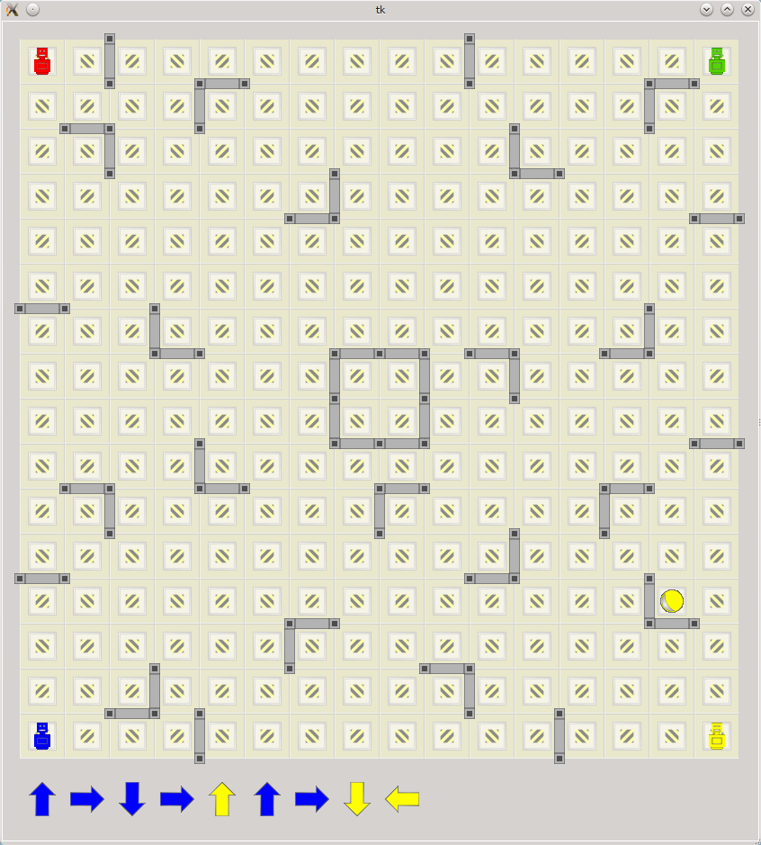
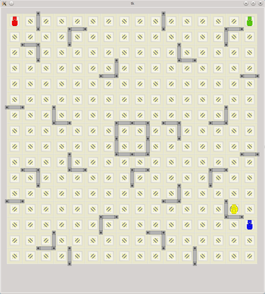
Figure 4: Visualization of solving goal(13) from initially cornered robots

The dimension of the board is fixed to $16$ in Line 1. As put forward by ?), barriers are indicated by atoms with predicate barrier/4. The first two arguments give the field position and the last two the orientation of the barrier, which is mostly east (1,0) or south (0,1). For instance, the atom barrier(2,1,1,0) in Line 3 represents the vertical wall between the fields (2,1) and (3,1), and barrier(5,1,0,1) stands for the horizontal wall separating (5,1) from (5,2).

⬇

dim(1..16).

barrier( 2, 1, 1,0). barrier(13,11, 1,0). barrier( 9, 7,0, 1).

barrier(10, 1, 1,0). barrier(11,12, 1,0). barrier(11, 7,0, 1).

barrier( 4, 2, 1,0). barrier(14,13, 1,0). barrier(14, 7,0, 1).

barrier(14, 2, 1,0). barrier( 6,14, 1,0). barrier(16, 9,0, 1).

barrier( 2, 3, 1,0). barrier( 3,15, 1,0). barrier( 2,10,0, 1).

barrier(11, 3, 1,0). barrier(10,15, 1,0). barrier( 5,10,0, 1).

barrier( 7, 4, 1,0). barrier( 4,16, 1,0). barrier( 8,10,0,-1).

barrier( 3, 7, 1,0). barrier(12,16, 1,0). barrier( 9,10,0,-1).

barrier(14, 7, 1,0). barrier( 5, 1,0, 1). barrier( 9,10,0, 1).

barrier( 7, 8, 1,0). barrier(15, 1,0, 1). barrier(14,10,0, 1).

barrier(10, 8,-1,0). barrier( 2, 2,0, 1). barrier( 1,12,0, 1).

barrier(11, 8, 1,0). barrier(12, 3,0, 1). barrier(11,12,0, 1).

barrier( 7, 9, 1,0). barrier( 7, 4,0, 1). barrier( 7,13,0, 1).

barrier(10, 9,-1,0). barrier(16, 4,0, 1). barrier(15,13,0, 1).

barrier( 4,10, 1,0). barrier( 1, 6,0, 1). barrier(10,14,0, 1).

barrier( 2,11, 1,0). barrier( 4, 7,0, 1). barrier( 3,15,0, 1).

barrier( 8,11, 1,0). barrier( 8, 7,0, 1).

Listing 14: The Board (board.lp)

Listing 15 gives the sixteen possible target locations printed on the game’s carton board (cf. Line 3 to 18). Each robot has four possible target locations, expressed by the ternary predicate target. Such a target is put in place via the unary predicate goal that associates a number with each location. The external declaration in Line 1 paves the way for fixing the target location from outside the solving process. For instance, setting goal(13) to true makes position (15,13) a target location for the yellow robot.

⬇

#external goal(1..16).

target(red, 5, 2) :- goal(1). % red moon

target(red, 15, 2) :- goal(2). % red triangle

target(green, 2, 3) :- goal(3). % green triangle

target(blue, 12, 3) :- goal(4). % blue star

target(yellow, 7, 4) :- goal(5). % yellow star

target(blue, 4, 7) :- goal(6). % blue saturn

target(green, 14, 7) :- goal(7). % green moon

target(yellow,11, 8) :- goal(8). % yellow saturn

target(yellow, 5,10) :- goal(9). % yellow moon

target(green, 2,11) :- goal(10). % green star

target(red, 14,11) :- goal(11). % red star

target(green, 11,12) :- goal(12). % green saturn

target(yellow,15,13) :- goal(13). % yellow star

target(blue, 7,14) :- goal(14). % blue star

target(red, 3,15) :- goal(15). % red saturn

target(blue, 10,15) :- goal(16). % blue moon

robot(red;green;blue;yellow).

#external pos((red;green;blue;yellow),1..16,1..16).

Listing 15: Robots and targets (targets.lp)

Similarly, the initial robot positions can be set externally, as declared in Line 21. That is, each robot can be put at 256 different locations. On the left hand side of Figure 4, we cornered all robots by setting pos(red,1,1), pos(blue,1,16), pos(green,16,1), and pos(yellow,16,16) to true.

Finally, the encoding in Listing 16 gives a non-incremental encoding with a fixed horizon, following the one by ?, Listing 2).

⬇

time(1..horizon).

dir(-1,0;1,0;0,-1;0,1).

stop( DX, DY,X, Y ) :- barrier(X,Y,DX,DY).

stop(-DX,-DY,X+DX,Y+DY) :- stop(DX,DY,X,Y).

pos(R,X,Y,0) :- pos(R,X,Y).

1 { move(R,DX,DY,T) : robot(R), dir(DX,DY) } 1 :- time(T).

move(R,T) :- move(R,_,_,T).

halt(DX,DY,X-DX,Y-DY,T) :- pos(_,X,Y,T), dir(DX,DY),

dim(X-DX), dim(Y-DY), not stop(-DX,-DY,X,Y), T < horizon.

goto(R,DX,DY,X,Y,T) :- pos(R,X,Y,T), dir(DX,DY), T < horizon.

goto(R,DX,DY,X+DX,Y+DY,T) :- goto(R,DX,DY,X,Y,T),

dim(X+DX), dim(Y+DY), not stop(DX,DY,X,Y), not halt(DX,DY,X,Y,T).

pos(R,X,Y,T) :- move(R,DX,DY,T), goto(R,DX,DY,X,Y,T-1),

not goto(R,DX,DY,X+DX,Y+DY,T-1).

pos(R,X,Y,T) :- pos(R,X,Y,T-1), time(T), not move(R,T).

:- target(R,X,Y), not pos(R,X,Y,horizon).

#show move/4.

Listing 16: Simple encoding for Ricochet Robots (ricochet.lp)

The first lines in Listing 16 furnish domain definitions, fixing the sequence of time steps (time/1) and two-dimensional representations of the four possible directions (dir/2). The constant horizon is expected to be provided via clingo option -c (e.g. ‘-c horizon=20’). Predicate stop/4 is the symmetric version of barrier/4 from above and identifies all blocked field transitions. The initial robot positions are fixed in Line 7 (in view of external input).

At each time step, some robot is moved in a direction (cf. Line 9). Such a move can be regarded as the composition of successive field transitions, captured by predicate goto/6 (in Line 15–17). To this end, predicate halt/5 provides temporary barriers due to robots’ positions before the move. To be more precise, a robot moving in direction (DX,DY) must halt at field (X-DX,Y-DY) when some (other) robot is located at (X,Y), and an instance of halt(DX,DY,X-DX,Y-DY,T) may provide information relevant to the move at step T+1 if there is no barrier between (X-DX,Y-DY) and (X,Y). Given this, the definition of goto/6 starts at a robot’s position (in Line 15) and continues in direction (DX,DY) (in Line 16–17) unless a barrier, a robot, or the board’s border is encountered. As this definition tolerates board traversals of length zero, goto/6 is guaranteed to yield a successor position for any move of a robot R in direction (DX,DY), so that the rule in Line 19–20 captures the effect of move(R,DX,DY,T). Moreover, the frame axiom in Line 21 preserves the positions of unmoved robots, relying on the projection move/2 (cf. Line 10).

Finally, we stipulate in Line 23 that a robot R must be at its target position (X,Y) at the last time point horizon. Adding directive ‘#show move/4.’ further allows for projecting stable models onto the extension of the move/4 predicate.

The encoding in Listing 16 allows us to decide whether a plan of length horizon exists. For computing a shortest plan, we may augment our decision encoding with an optimization directive. This can be accomplished by adding the part in Listing 17.

⬇

goon(T) :- target(R,X,Y), T = 0..horizon, not pos(R,X,Y,T).

:- move(R,DX,DY,T-1), time(T), not goon(T-1), not move(R,DX,DY,T).

#minimize{ 1,T : goon(T) }.

Listing 17: Encoding part for optimization (optimization.lp)

The rule in Line 27 indicates whether some goal condition is (not) established at a time point. Once the goal is established, the additional integrity constraint in Line 29 ensures that it remains satisfied by enforcing that the goal-achieving move is repeated at later steps (without altering robots’ positions). Note that the #minimize directive in Line 31 aims at few instances of goon/1, corresponding to an early establishment of the goal, while further repetitions of the goal-achieving move are ignored. Our extended encoding allows for computing a shortest plan of length bounded by horizon. If there is no such plan, the problem can be posed again with an enlarged horizon. For computing a shortest plan in an unbounded fashion, we can take advantage of incremental ASP solving, as illustrated in Section 5.1.

Apart from the two external directives that allow us to vary initial robot and target positions, the four programs constitute an ordinary ASP formalization of a Ricochet Robots instance. To illustrate this, let us override the external directives by adding facts accounting for the robot and target positions on the left hand side of Figure 4. The corresponding call of clingo is shown in Listing 20.

⬇

clingo board.lp targets.lp ricochet.lp optimization.lp \

-c horizon=10 \

<(echo "pos(red,1,1). pos(green,16,1). \

pos(blue,1,16). pos(yellow,16,16). \

goal(13).")

Listing 18: One-shot solving with clingo

⬇

move(blue,0,-1,1) move(blue,1,0,2) move(blue,0,1,3) \

move(blue,1,0,4) move(yellow,0,-1,5) move(blue,0,-1,6) \

move(blue,1,0,7) move(yellow,0,1,8) move(yellow,-1,0,9) \

move(yellow,-1,0,10)

Listing 19: Stable model projected onto the extension of the move/4 predicate

The resulting one-shot solving process yields a(n optimal) stable model containing the extension of the move/4 predicate given in Listing 19. The move atoms in Line 1–4 of Listing 19 correspond to the plan indicated by the colored arrows at the bottom of the left hand side of Figure 4. That is, the blue robot starts by going north, east, south, and east, then the yellow one goes north, the blue one resumes and goes north and east, before finally the yellow robot goes south (bouncing off the blue one) and lands on the target by going west. This leads to the situation depicted on the right hand side of Figure 4. Note that the tenth move (in Line 4) is redundant since it merely replicates the previous one because the goal was already reached after nine steps.

5.3.2 Playing in rounds

Ricochet Robots is played in rounds. Hence, the next goal must be reached with robots placed at the positions resulting from the previous round. For example, when pursuing goal(4) in the next round, the robots must start from the end positions given on the right hand side of Figure 4. The resulting configuration is shown on the left hand side of Figure 5.

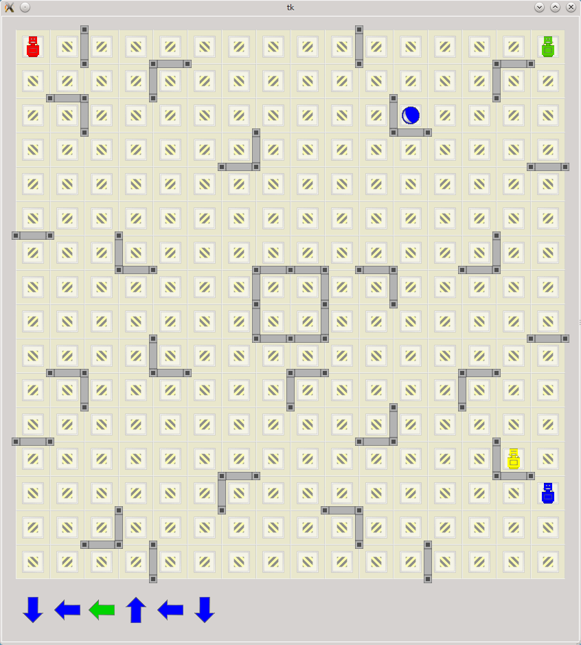
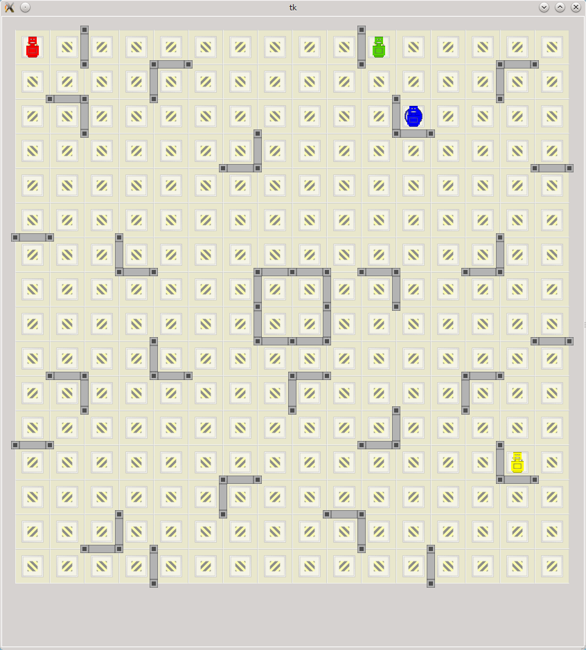
Figure 5: Visualization of solving goal(4) from robot positions after having solved goal(13)

For one-shot solving, we would re-launch clingo from scratch as shown in Listing 20, yet by accounting for the new target and robot positions by replacing Line 3–5 of Listing 20 by the following ones.

⬇

<(echo "pos(red,1,1). pos(green,16,1). \

pos(blue,16,10). pos(yellow,15,13). \

goal(4)." )

Listing 20: One-shot solving with clingo

Unlike this, our multi-shot approach to playing in rounds relies upon a single operational clingo control object that we use in a simple loop:

1. Create an operational control object (containing a grounder and a solver object)

2. Load and ground the programs in Listing 14, 15, 16, and optionally 17
   (relative to some fixed horizon) within the control object

3. While there is a goal, do the following

   1. Enforce the initial robot positions

   2. Enforce the current goal

   3. Solve the logic program contained in the control object

The control loop is implemented in Python by means of clingo’s Python API. This module provides grounding and solving functionalities. As mentioned in Section 2, both modules support (almost) literal counterparts to ‘Create’, ‘Load’, ‘Ground’, and ‘Solve’. The “enforcement” of robot and target positions is more complex, as it involves changing the truth values of externally controlled atoms (mimicking the insertion and deletion of atoms, respectively).

The resulting Python program is given in Listing 21.

⬇

from clingo import Control, Model, Function

class Player:

def __init__(self, horizon, positions, files):

self.last_positions = positions

self.last_solution = None

self.undo_external = []

self.horizon = horizon

self.ctl = Control(

[’-c’, ’horizon={0}’.format(self.horizon)])

for x in files:

self.ctl.load(x)

self.ctl.ground([("base", [])])

def solve(self, goal):

for x in self.undo_external:

self.ctl.assign_external(x, False)

self.undo_external = []

for x in self.last_positions + [goal]:

self.ctl.assign_external(x, True)

self.undo_external.append(x)

self.last_solution = None

self.ctl.solve(on_model=self.on_model)

return self.last_solution

def on_model(self, model):

self.last_solution = model.symbols(atoms=True)

self.last_positions = []

for atom in model.symbols(atoms=True):

if (atom.name == "pos" and

len(atom.arguments) == 4 and

atom.arguments[3].number == self.horizon):

self.last_positions.append(

Function("pos", atom.arguments[:-1]))

horizon = 15

encodings = ["board.lp", "targets.lp", "ricochet.lp", "optimization.lp"]

positions = [Function("pos", [Function("red"), 1, 1]),

Function("pos", [Function("blue"), 1, 16]),

Function("pos", [Function("green"), 16, 1]),

Function("pos", [Function("yellow"), 16, 16])]

sequence = [Function("goal", [13]),

Function("goal", [4]),

Function("goal", [7])]

player = Player(horizon, positions, encodings)

for goal in sequence:

print player.solve(goal)

Listing 21: The Ricochet Robot Player (ricochet.py)

Line 1 imports the clingo module. We are only using three classes from the module, which we directly pull into the global namespace to avoid qualification with “clingo.” and so to keep the code compact.

Line 3–34 show the Player class. This class encapsulates all state information including clingo’s Control object that in turn holds the state of the underlying grounder and solver. In the Player’s __init__ function (similar to a constructor in other object-oriented languages) the following member variables are initialized:

last_positions

This variable is initialized upon construction with the starting positions of the robots. During the progression of the game, this variable holds the initial starting positions of the robots for each turn.

last_solution

This variable holds the last solution of a search call.

undo_external

We want to successively solve a sequence of goals. In each step, a goal has to be reached from different starting positions. This variable holds a list containing the current goal and starting positions that have to be cleared upon the next step.

horizon

We are using a bounded encoding. This (Python) variable holds the maximum number of moves to find a solution for a given step.

ctl

This variable holds the actual object providing an interface to the grounder and solver. It holds all state information necessary for multi-shot solving along with heuristic information gathered during solving.

As shown in Line 4–13, the constructor takes the horizon, initial robot positions, and the files containing the various logic programs. clingo’s Control object is created in Line 9–10 by passing the option -c to replace the logic program constant horizon by the value of the Python variable horizon during grounding. Finally, the constructor loads all files and grounds the entire logic program in Line 11–13. Recall from Section 2 that all rules outside the scope of #program directives belong to the base program. Note also that this is the only time grounding happens because the encoding is bounded. All following solving steps are configured exclusively via manipulating external atoms.

The solve method in Line 15–24 starts with initializing the search for the solution to the new goal. To this end, it first undos in Line 16–17 the previous goal and starting positions stored in undo_external by assigning False to the respective atoms. In the following lines 19 to 21, the next step is initialized by assigning True to the current goal along with the last robot positions; these are also stored in undo_external so that they can be taken back afterwards. Finally, the solve method calls clingo’s ctl.solve to initiate the search. The result is captured in variable last_solution. Note that the call to ctl.solve takes ctl.on_model as (keyword) argument, which is called whenever a model is found. In other words, on_model acts as a callback for intercepting models. Finally, variable last_solution is returned at the end of the method.

The last function of the Player class is the on_model callback. As mentioned, it intercepts the (final) models computed by the solver, which can then be inspected via the functions of the Model class. At first, it stores the shown atoms in variable last_solution in Line 27. The remainder of the on_model callback extracts the final robot positions from the stable model. For that, it loops in Line 29–34 over the full set of atoms in the model and checks whether their signatures match. That is, if an atom is formed from predicate pos/4 and its fourth argument equals the horizon, then it is appended to the list of last_positions after stripping its time step from its arguments.

As an example, consider pos(yellow,15,13,20), say the final position of the yellow robot on the right hand side of Figure 4 at an horizon of 20. This leads to the addition of pos(yellow,15,13) to the last_positions. Note that pos(yellow,15,13) is declared an external atom in Line 21 of Listing 15. For playing the next round, we can thus make it True in Line 20 of Listing 21. And when solving, the rule in Line 7 of Listing 16 allows us to derive pos(yellow,15,13,0) and makes it the new starting position of the yellow robot, as shown on the left hand side of Figure 5.

Line 36–44 show the code for configuring the player. They set the search horizon, the encodings to solve with, and the initial positions in form of clingo terms. Furthermore, we fix a sequence of goals in Line 42–44. In a more realistic setting, either some user interaction or a random sequence might be generated to emulate arbitrary draws.

⬇

python ricochet.py

[move(red,0,1,1), move(red,1,0,2), move(red,0,1,3), ...]

[move(blue,0,-1,1), move(blue,1,0,2), move(blue,0,1,3), ...]

[move(green,0,1,1), move(green,1,0,2), move(green,1,0,3), ...]

Listing 22: Multi-shot solving with clingo’s Python API

Finally, Line 46–48 implement the search for sequences of moves that solve the configuration given above. For each goal in the sequence, a solution is plainly printed, as engaged in Line 48. The three lists in Listing 24 represent solutions to the three goals in Line 42–44. The clingo library does not foresee any output, which must thus be handled by the scripting language. Note also that the first list represents an alternative solution to the one given in Listing 19.

5.4 Optimization

Another innovative feature of clingo is its incremental optimization. This allows for adapting objective functions along the evolution of a program at hand. A simple example is the search for shortest plans when increasing the horizon in non-consecutive steps. To see this, recall that literals in minimize statements (and analogously weak constraints) are supplied with a sequence of terms of the form $w@p,\vec{t}$, where $w$ and $p$ are integers providing a weight and a priority level and $\vec{t}$ is a sequence of terms (cf. [Calimeri et al. (2012)]). As an example, consider the subprogram:

⬇

#program cumulativeObjective(t).

#minimize{ W@P,X,Y,t : move(X,Y,W,P,t) }.

Listing 23: Multi-shot solving with clingo’s Python API

When grounding and solving cumulativeObjective(t) for successive values of t, the solver’s objective function (per priority level P) is gradually extended with new atoms over move/5, and all previous ones are kept.

For enabling the removal of literals from objective functions, we can use externals:

⬇

#program volatileObjective(t).

#external activateObjective(t).

#minimize{ W@P,X,Y,t : move(X,Y,W,P,t), activateObjective(t) }.

Listing 24: Multi-shot solving with clingo’s Python API

The subprogram volatileObjective(t) behaves like cumulativeObjective(t) as long as the external atom activateObjective(t) is true. Once it is set to false, all atoms over move/5 with the corresponding term for t are dismissed from objective functions.

6 Application program interfaces

This section provides some further selected functionalities of clingo’s APIs; detailed descriptions can be found at potassco.org. Currently, clingo provides APIs in C, C++, Lua, and Python, all sharing the same functionality. A tutorial on using the Python API for multi-shot and theory solving was given by ?).

The theory reasoning capabilities of clingo are described by ?). In brief, clingo provides generic means for incorporating theory reasoning. They span from theory grammars for seamlessly extending its input language with theory expressions to a simple interface for integrating theory propagators into its solver component. Multi-shot solving for selected theories is described by ?) and ?).

The central role in multi-shot solving is played by control objects capturing the system states of grounders and solvers, as introduced in Section 4.5. While the control object created by invoking clingo from the command line is passed as argument to the main routine, further such objects can be created with the constructor Control. Examples for both settings can be found in Line 8 of Listing 7 and Line 9 and 10 of Listing 21, respectively. In general, this allows multiple independent clingo objects to coexist and communicate with each other.

clingo’s interface can be structured into three parts.

Parsing.

A simple but very useful feature of clingo’s API is that it allows us to leverage the parser of its grounding component gringo to obtain an abstract syntax tree (AST) of the non-ground program. More precisely, the interface allows for both obtaining an AST of a full-fledged logic program and adding such a program in form of an AST. This provides an easy way of applying program transformations on the non-ground level without any burden of parsing input programs in their full generality. This feature is exploited by the systems asprin [Brewka et al. (2015b)] for expressing preferences and anthem for formula extraction.

Grounding.

A basic functionality of clingo objects is to incrementally augment non-ground programs by loading programs from file or adding them in string form. An example of the former can be found in Line 12 of Listing 21; the latter is accomplished by the counterpart of add, defined in Section 4.5. Notably, this functionality allows for adding dynamically generated programs.

More fine-grained control is provided by the low level part of the interface. This allows, for instance, for inspecting the result of grounding and adding ground rules in the intermediate ASP format aspif (cf. [Kaminski et al. (2017)]). In this way, one can iterate over all ground atoms and inspect them individually, or implement eager constraint translations by adding new (theory) atoms on demand. Also, symbols can be injected during grounding via external functions, similar to value invention [Calimeri et al. (2007)].

Solving.

The principal solve method can be shaped in various ways. For instance, we have seen in Listing 21 how on_model can act as a callback for intercepting models. More precisely, for each stable model found during a call to solve(on_model=f), a model object is passed to function f, whose implementation can then access and inspect the model. An example consists of the addition of constraints whenever a model is found, as in optimization tasks, or final tests on model candidates. Similarly, solve can by supplied with assumptions, as detailed in (30). For instance, the call solve(assumptions=[(Function("a"), True)]) only admits stable models containing atom a. Moreover, clingo provides an asynchronous interface, which is particularly useful in reactive settings. Here, solving is done in the background and interruptible at any time. For example, this allows to accommodate scenarios where agents have to stay responsive even though solving has not yet finished. Finally, it is worth mentioning that dedicated parts of the API allow for configurating search and extracting solver statistics. In combination with the aforementioned on_model callback this allows for re-configuring search in view of the statistics gathered during the search for the last model.

7 Experiments

The computational advantage of multi-shot solving lies in its avoidance of redundancies otherwise caused by relaunching grounder and solver programs. Since the substantial savings on grounding intense benchmarks have already been demonstrated [Gebser et al. (2008)], we focus our empirical analysis on the impact of our approach on solving. In particular, we want to investigate in how far multi-shot solving can benefit from the learning capacities of modern ASP solvers and the reuse of already gathered heuristic scores. To this end, we empirically evaluate the impact of clingo’s multi-shot solving capacities on three planning benchmarks: Towers of Hanoi (cf. Section 5.1), Ricochet Robots (cf. Section 5.3), and ASP encodings of PDDL problems [Dimopoulos et al. (2017)]. For either benchmark, we let clingo version 4.5.4 search for a shortest plan by incrementally extending the horizon until the first plan is found. In particular, we consider multi-shot solving by means of clingo’s built-in incremental mode (invoked by ‘#include <incmode>.’) in four different settings:

• multi: keeping recorded nogoods as well as heuristic values between solver calls

• multi -heuristic: keeping recorded nogoods, but not heuristic values, between solver calls

• multi -nogoods: keeping heuristic values, but not recorded nogoods, between solver calls

• multi -heuristic -nogoods: keeping neither recorded nogoods nor heuristic values between solver calls

We contrast these four settings to the traditional single-shot approach, denoted by single, where clingo performs grounding and solving from scratch for each planning horizon. The experiments were run sequentially on a Linux machine equipped with Xeon E5520 2.27GHz processors, limiting wall-clock time to 3000 seconds per run without imposing any (effective) memory limit. clingo was run in all experiments in its default configuration except for the option --forget-on-step that allows for configuring the four settings above.

We portray our results in terms of cactus plots, in which the x-axes list instances ordered by time (and conflicts) and the y-axes reflect times and conflicts, respectively. The magnitude of the latter are given on top of the y-axis.

7.1 Towers of Hanoi

Figure 6: Cactus plots for Towers of Hanoi benchmark

The upper plot in Figure 6 displays runtimes for each clingo setting in increasing order over 45 instances of the Towers of Hanoi benchmark. Most apparently, we observe that single-shot solving performed in the single setting fails to complete any of the instances within the allotted 3000 seconds. This clearly shows that the redundancy of relaunching grounding and solving processes from scratch for each horizon incurs non-negligible overhead here.

Somewhat unexpectedly, the multi-shot solving approaches in which recorded nogoods are discarded between successive solver calls, viz. multi -nogoods and multi -heuristic -nogoods, perform much better than single-shot solving and complete all 45 instances within the time limit. On the one hand, this advantage is owed to incremental grounding, adding only new rule instances when switching from one horizon to the next. On the other hand, we verified that solving steps take the major share of runtime with each setting, and the numbers of conflicts plotted in the lower part of Figure 6 exhibit substantial search reductions in multi-shot solving, even when neither recorded nogoods nor heuristic values are kept. In fact, at the implementation level clingo asserts unary nogoods and stores binary as well as ternary nogoods persistently in dedicated data structures. Hence, such short nogoods remain available in multi-shot solving regardless of settings and explain the gap to iterated single-shot solving, where respective information has to be repeatedly retrieved from search conflicts at each solving step.

Keeping also long nogoods between solver calls, as done in the multi and multi -heuristic settings, further reduces search conflicts and runtime by a factor of about 5 or 1.5, respectively. This indicates a trade-off between memory demands and search savings due to recorded nogoods, where the savings outweigh the overhead on the Towers of Hanoi benchmark. Unlike that, keeping heuristic values does not pay off here, and the two -heuristic settings save some fraction of runtime in comparison to their counterparts passing such values between solver calls. Although respective gaps are modest, we conclude that biasing search to proceed as in previous solving steps does not provide shortcuts for problems with an extended planning horizon.

7.2 Ricochet Robots

Figure 7: Cactus plots for Ricochet Robots benchmark

The behavior of single- and multi-shot solving approaches on 38 instances of the Ricochet Robots benchmark, plotted in Figure 7, parallels the previous observations. While the single setting is able to complete 22 of the instances within the given time, the most successful multi-shot solving approach, multi -heuristic -nogoods, solves all of them. In contrast to Towers of Hanoi above, keeping long nogoods does not pay off here, as the lower plot in Figure 7 shows that they do not significantly reduce the search conflicts at solving steps with an extended horizon. Hence, the two -nogoods settings are ahead in terms of runtime as well as solved instances displayed in the upper part of Figure 7. Moreover, we see that keeping or discarding heuristic values, the latter denoted by -heuristic, does not make much difference, which again exposes that biasing the search process in view of previous solving steps does not necessarily help for problem extensions.

7.3 PDDL Problems

Figure 8: Cactus plots for PDDL benchmark

The performance results displayed in Figure 8, summarizing 20 instances obtained by translating planning problems from PDDL, also exhibit a significant gap separating single-shot from multi-shot solving in its four settings. The behavior of the latter differs primarily w.r.t. the treatment of long nogoods, where only the two -nogoods settings that discard them between solver calls complete all instances in time. In fact, comparing runtimes in the upper and numbers of conflicts in the lower part of Figure 8, it turns out that keeping such long nogoods incurs overhead without bringing about (consistent) search savings in return. The reduced numbers of conflicts relative to single-shot solving nevertheless indicate a substantial added value of keeping some nogoods, in particular, short ones, between solver calls.

7.4 Observations

On all benchmarks the number of conflicts is lower in the multi settings compared to the single one. This is due to the reuse of nogoods learnt from previous solving steps. In fact, the treatment of nogoods had the greatest influence on the runtime in the multi settings. As regards long nogoods, the sometimes unproportional overhead of keeping them, observed on the Ricochet Robots benchmark and PDDL problems, suggests to strive in the future for adaptive filtering mechanisms (beyond regular nogood deletion) assessing the relevance of recorded nogoods from previous solving steps. Unlike that, clingo settings that differ in the treatment of heuristic values only, i.e., pairs denoted with or without -heuristic, exhibit comparable behavior on all three investigated benchmark problems, thus indicating that recorded nogoods play a more important role upon successive solver calls.

Our benchmarks were not very memory demanding. The peak memory consumption over all benchmarks was 187 MB when multi-shot solving and only 150 MB in the single-shot setting. Even though it might seem that the single-shot approach has a smaller memory footprint, the multi-shot settings probably just held larger databases of learnt clauses leading to a slightly higher memory consumption. With the selected benchmarks, the memory used by the grounding component is negligible.

8 Related work

Although clingo [Gebser et al. (2011)] already featured Lua as an embedded scripting language up to series 3, its usage was limited to (deterministic) computations during grounding; neither were library functions furnished by clingo 3.

Of particular interest is dlvhex [Eiter et al. (2012)], an ASP system aiming at the integration of external computation sources. For this purpose, dlvhex relies on higher-order logic programs using external higher-order atoms for software interoperability. Such external atoms should not be confused with clingo’s #external directive because they are evaluated via procedural means during solving. Given this, dlvhex can be seen as an ASP modulo Theory solver, similar to SAT modulo Theory solvers [Nieuwenhuis et al. (2006)]. In fact, dlvhex is build upon clingo and follows the design of the ASP modulo CSP solver clingcon [Ostrowski and Schaub (2012)] in communicating with external “oracles” through clasp’s post propagation mechanism. In this way, theory solvers are tightly integrated into the ASP system and have access to the solver’s partial assignments. Unlike this, multi-shot solving only provides access to total (stable) assignments. This is why clingo also offers full-fledged theory reasoning capabilities, dealing with partial assignments [Gebser et al. (2016), Kaminski et al. (2017)]. Clearly, the above considerations also apply to extensions of dlvhex, such as acthex [Fink et al. (2013)]. Furthermore, jdlv [Febbraro et al. (2012)] encapsulates the dlv system to facilitate one-shot ASP solving in Java environments by providing means to generate and process logic programs, and to afterwards extract their stable models. embasp [Fuscà et al. (2016)] provides a more recent and more general environment for embedding ASP systems, including clingo and dlv, into external systems. Meanwhile the ASP solver wasp [Alviano et al. (2015)] also features a foreign language API, yet restricted to solving functionalities. More precisely, it provides low-level functionalities to customize heuristics and propagation [Dodaro et al. (2016), Dodaro et al. (2016)].

The procedural attachment to the idp system [De Pooter et al. (2013), De Cat et al. (2014)] builds on interfaces to C++ and Lua. Like clingo, it allows for evaluating functions during grounding, calling the grounder and solver multiple times, inspecting solutions, and reacting to external input after search. The emphasis, however, lies on high-level control blending in with idp’s modeling language, while clingo offers more fine-grained control over the grounding and solving process, particularly aiming at a flexible incremental assembly of programs from subprograms.

In SAT, incremental solver interfaces from low-level APIs are common practice. Pioneering work was done in minisat [Eén and Sörensson (2004)], furnishing a C++ interface for solving under assumptions. In fact, the clasp library underlying clingo builds upon this functionality to implement incremental search (see [Gebser et al. (2008)]). Given that SAT deals with propositional formulas only, solvers and their APIs lack support for modeling languages and grounding. Unlike this, the SAT modulo Theory solver z3 [de Moura and Bjørner (2008)] comes with a Python API that, similar to clingo, provides a library for controlling the solver as well as language bindings for constraint handling. In this way, Python can be used as a modeling language for z3.

9 Conclusion

The clingo system complements ASP’s declarative input language by control capacities expressed either by embedded scripting languages or by importing clingo modules into imperative programs. This is accomplished within a single integrated ASP grounding and solving process in which a logic program may evolve over time. The addition, deletion, and replacement of programs is controlled procedurally by means of clingo’s API. Applications that cannot be captured with the standard one-shot approach of ASP but that require evolving logic programs are manifold. Examples include unrolling a transition function as in planning, interacting with an environment as in assisted living, robotics, or stream reasoning, interacting with a user exploring a domain, theory solving, and advanced forms of search. Addressing these demands by providing a high-level API yields a generic and transparent approach. Unlike this, previous systems, like iclingo and oclingo, had a dedicated purpose involving rigid control procedures buried in monolithic programs. Rather than that, the basic technology of clingo allows us to instantiate subprograms in-between solver invocations in a fully customizable way. On the declarative side, the availability of program parameters and the embedding of #external directives into the grounding process provide us with a great flexibility in modeling schematic subprograms. In addition, the possibility of assigning input atoms facilitates the implementation of applications such as query answering [Gebser et al. (2013)] or sliding window reasoning [Gebser et al. (2012)], as truth values can now be switched without modifying logic programs.

The semantic underpinnings of our framework in terms of module theory capture the dynamic combination of logic programs in a generic way. Although this eases the modular composition of data structures, other choices are possible at the cost of higher maintenance. Note that the difficulty of composing subprograms in ASP is due to its nonmonotonic nature; this is much easier in monotonic approach such as SAT. Finally, it is interesting future work to investigate how dedicated change operations that were so far only of theoretic interest, like updating [Alferes et al. (2002)], forgetting [Zhang and Foo (2006)], revising [Delgrande et al. (2008)], or merging [Delgrande et al. (2009)] etc., can be put into practice within this framework. A first attempt at capturing the update of logic programs was made by ?).

The input language of clingo extends the ASP-Core-2 standard [Calimeri et al. (2012)] and has meanwhile been put in its entirety on solid semantic foundations [Gebser et al. (2015)]. Although we have presented clingo for normal logic programs, we mention that it accepts (extended) disjunctive logic programs processed via the multi-threaded solving approach of clasp [Gebser et al. (2013)]. Since clingo embeds clasp series 3, it moreover features domain-specific heuristics [Gebser et al. (2013)] and optimization using unsatisfiable cores [Andres et al. (2012)]. clingo is freely available at potassco.org, and its releases include many best practice examples illustrating the aforementioned application scenarios.

Since its first release and accompanying publication [Gebser et al. (2014)], clingo’s multi-shot solving framework has been used for implementing several ASP-based reasoning systems, such as asprin [Brewka et al. (2015a), Brewka et al. (2015b)], aspic [Gebser et al. (2013)], rosoclingo [Andres et al. (2015)], and dflat [Abseher et al. (2014)]; various forms of aggregates were implemented with it by ?) and ?). As well, dlvhex [Eiter et al. (2012)] builds upon clingo and its versatile API. This already hints at the potential impact of clingo’s multi-shot ASP solving framework, and we believe that it constitutes a step towards putting more and more applications into the reach of ASP.

Multi-shot ASP solving broadens the spectrum of applications of ASP. This also brings about the new user profile of ASP engineering that combines ASP modeling with traditional programming for controlling an ASP solving process. This may lead to generic advanced forms of ASP solving such as the incremental approach in Section 5.1 or be restricted to customized settings as with the Ricochet Robots game in Section 5.3. Multi-shot solving enables users to engineer such novel declarative systems on top of ASP. We believe that this new engineering facet is crucial to putting ASP into practice.

Acknowledgments.

We are grateful to Evgenii Balai, Javier Romero, and Adam Smith for many fruitful discussions on the paper. This work was partially funded by DFG grant SCHA 550/9.

References

- Abiteboul et al. (1995) Abiteboul, S., Hull, R., and Vianu, V. 1995. Foundations of Databases. Addison-Wesley.
- Abseher et al. (2014) Abseher, M., Bliem, B., Charwat, G., Dusberger, F., Hecher, M., and Woltran, S. 2014. The D-FLAT system for dynamic programming on tree decompositions. In Proceedings of the Fourteenth European Conference on Logics in Artificial Intelligence (JELIA’14), E. Fermé and J. Leite, Eds. Lecture Notes in Artificial Intelligence, vol. 8761. Springer-Verlag, 558–572.
- Alferes et al. (2002) Alferes, J., Pereira, L., Przymusinska, H., and Przymusinski, T. 2002. LUPS: A language for updating logic programs. Artificial Intelligence 138, 1-2, 87–116.
- Alviano et al. (2015) Alviano, M., Dodaro, C., Leone, N., and Ricca, F. 2015. Advances in WASP. See Calimeri et al. (2015), 40–54.
- Alviano et al. (2015) Alviano, M., Faber, W., and Gebser, M. 2015. Rewriting recursive aggregates in answer set programming: Back to monotonicity. Theory and Practice of Logic Programming 15, 4-5, 559–573. Available at http://arxiv.org/abs/1507.03923.
- Alviano and Leone (2015) Alviano, M. and Leone, N. 2015. Complexity and compilation of GZ-aggregates in answer set programming. Theory and Practice of Logic Programming 15, 4-5, 574–587.
- Andres et al. (2012) Andres, B., Kaufmann, B., Matheis, O., and Schaub, T. 2012. Unsatisfiability-based optimization in clasp. In Technical Communications of the Twenty-eighth International Conference on Logic Programming (ICLP’12), A. Dovier and V. Santos Costa, Eds. Vol. 17. Leibniz International Proceedings in Informatics (LIPIcs), 212–221.
- Andres et al. (2015) Andres, B., Rajaratnam, D., Sabuncu, O., and Schaub, T. 2015. Integrating ASP into ROS for reasoning in robots. See Calimeri et al. (2015), 69–82.
- Balduccini and Janhunen (2017) Balduccini, M. and Janhunen, T., Eds. 2017. Proceedings of the Fourteenth International Conference on Logic Programming and Nonmonotonic Reasoning (LPNMR’17). Lecture Notes in Artificial Intelligence, vol. 10377. Springer-Verlag.
- Banbara et al. (2017) Banbara, M., Kaufmann, B., Ostrowski, M., and Schaub, T. 2017. Clingcon: The next generation. Theory and Practice of Logic Programming 17, 4, 408–461.
- Baral (2003) Baral, C. 2003. Knowledge Representation, Reasoning and Declarative Problem Solving. Cambridge University Press.
- Brewka et al. (2015a) Brewka, G., Delgrande, J., Romero, J., and Schaub, T. 2015a. asprin: Customizing answer set preferences without a headache. In Proceedings of the Twenty-Ninth National Conference on Artificial Intelligence (AAAI’15), B. Bonet and S. Koenig, Eds. AAAI Press, 1467–1474.
- Brewka et al. (2015b) Brewka, G., Delgrande, J., Romero, J., and Schaub, T. 2015b. Implementing preferences with asprin. See Calimeri et al. (2015), 158–172.
- Brewka et al. (2012) Brewka, G., Eiter, T., and McIlraith, S., Eds. 2012. Proceedings of the Thirteenth International Conference on Principles of Knowledge Representation and Reasoning (KR’12). AAAI Press.
- Cabalar and Son (2013) Cabalar, P. and Son, T., Eds. 2013. Proceedings of the Twelfth International Conference on Logic Programming and Nonmonotonic Reasoning (LPNMR’13). Lecture Notes in Artificial Intelligence, vol. 8148. Springer-Verlag.
- Calimeri et al. (2007) Calimeri, F., Cozza, S., and Ianni, G. 2007. External sources of knowledge and value invention in logic programming. Annals of Mathematics and Artificial Intelligence 50, 3-4, 333–361.
- Calimeri et al. (2012) Calimeri, F., Faber, W., Gebser, M., Ianni, G., Kaminski, R., Krennwallner, T., Leone, N., Ricca, F., and Schaub, T. 2012. ASP-Core-2: Input language format. Available at https://www.mat.unical.it/aspcomp2013/ASPStandardization.
- Calimeri et al. (2015) Calimeri, F., Ianni, G., and Truszczyński, M., Eds. 2015. Proceedings of the Thirteenth International Conference on Logic Programming and Nonmonotonic Reasoning (LPNMR’15). Lecture Notes in Artificial Intelligence, vol. 9345. Springer-Verlag.
- De Cat et al. (2014) De Cat, B., Bogaerts, B., Bruynooghe, M., and Denecker, M. 2014. Predicate logic as a modelling language: The IDP system. CoRR abs/1401.6312.
- de Moura and Bjørner (2008) de Moura, L. and Bjørner, N. 2008. Z3: An efficient SMT solver. In Proceedings of the Fourteenth International Conference on Tools and Algorithms for the Construction and Analysis of Systems (TACAS’08), C. Ramakrishnan and J. Rehof, Eds. Lecture Notes in Computer Science, vol. 4963. Springer-Verlag, 337–340.
- De Pooter et al. (2013) De Pooter, S., Wittocx, J., and Denecker, M. 2013. A prototype of a knowledge-based programming environment. In Proceedings of the Nineteenth International Conference on Applications of Declarative Programming and Knowledge Management (INAP’11) and the Twenty-fifth Workshop on Logic Programming (WLP’11), H. Tompits, S. Abreu, J. Oetsch, J. Pührer, D. Seipel, M. Umeda, and A. Wolf, Eds. Lecture Notes in Computer Science, vol. 7773. Springer-Verlag, 279–286.
- Delgrande and Faber (2011) Delgrande, J. and Faber, W., Eds. 2011. Proceedings of the Eleventh International Conference on Logic Programming and Nonmonotonic Reasoning (LPNMR’11). Lecture Notes in Artificial Intelligence, vol. 6645. Springer-Verlag.
- Delgrande et al. (2008) Delgrande, J., Schaub, T., Tompits, H., and Woltran, S. 2008. Belief revision of logic programs under answer set semantics. In Proceedings of the Eleventh International Conference on Principles of Knowledge Representation and Reasoning (KR’08), G. Brewka and J. Lang, Eds. AAAI Press, 411–421.
- Delgrande et al. (2009) Delgrande, J., Schaub, T., Tompits, H., and Woltran, S. 2009. Merging logic programs under answer set semantics. In Proceedings of the Twenty-fifth International Conference on Logic Programming (ICLP’09), P. Hill and D. Warren, Eds. Lecture Notes in Computer Science, vol. 5649. Springer-Verlag, 160–174.
- Dimopoulos et al. (2017) Dimopoulos, Y., Gebser, M., Lühne, P., Romero, J., and Schaub, T. 2017. plasp 3: Towards effective ASP planning. See Balduccini and Janhunen (2017), 286–300.
- Dodaro et al. (2016) Dodaro, C., Gasteiger, P., Leone, N., Musitsch, B., Ricca, F., and Schekotihin, K. 2016. Driving CDCL search. CoRR abs/1611.05190.
- Dodaro et al. (2016) Dodaro, C., Ricca, F., and Schüller, P. 2016. External propagators in wasp: Preliminary report. In Proceedings of the Twenty-third International Workshop on Experimental Evaluation of Algorithms for Solving Problems with Combinatorial Explosion (RCRA’16). Vol. 1745. CEUR Workshop Proceedings, 1–9.
- Eén and Sörensson (2003) Eén, N. and Sörensson, N. 2003. Temporal induction by incremental SAT solving. Electronic Notes in Theoretical Computer Science 89, 4.
- Eén and Sörensson (2004) Eén, N. and Sörensson, N. 2004. An extensible SAT-solver. In Proceedings of the Sixth International Conference on Theory and Applications of Satisfiability Testing (SAT’03), E. Giunchiglia and A. Tacchella, Eds. Lecture Notes in Computer Science, vol. 2919. Springer-Verlag, 502–518.
- Eiter et al. (2012) Eiter, T., Fink, M., Krennwallner, T., and Redl, C. 2012. Conflict-driven ASP solving with external sources. Theory and Practice of Logic Programming 12, 4-5, 659–679.
- Febbraro et al. (2012) Febbraro, O., Leone, N., Grasso, G., and Ricca, F. 2012. JASP: A framework for integrating answer set programming with Java. See Brewka et al. (2012), 541–551.
- Fink et al. (2013) Fink, M., Germano, S., Ianni, G., Redl, C., and Schüller, P. 2013. ActHEX: Implementing HEX programs with action atoms. See Cabalar and Son (2013), 317–322.
- Fuscà et al. (2016) Fuscà, D., Germano, S., Zangari, J., Anastasio, M., Calimeri, F., and Perri, S. 2016. A framework for easing the development of applications embedding answer set programming. In Proceedings of the Eighteenth International Symposium on Principles and Practice of Declarative Programming (PPDP’16), J. Cheney and G. Vidal, Eds. ACM Press, 38–49.
- Gebser et al. (2012) Gebser, M., Grote, T., Kaminski, R., Obermeier, P., Sabuncu, O., and Schaub, T. 2012. Stream reasoning with answer set programming: Preliminary report. See Brewka et al. (2012), 613–617.
- Gebser et al. (2011) Gebser, M., Grote, T., Kaminski, R., and Schaub, T. 2011. Reactive answer set programming. See Delgrande and Faber (2011), 54–66.
- Gebser et al. (2015) Gebser, M., Harrison, A., Kaminski, R., Lifschitz, V., and Schaub, T. 2015. Abstract Gringo. Theory and Practice of Logic Programming 15, 4-5, 449–463. Available at http://arxiv.org/abs/1507.06576.
- Gebser et al. (2013) Gebser, M., Jost, H., Kaminski, R., Obermeier, P., Sabuncu, O., Schaub, T., and Schneider, M. 2013. Ricochet robots: A transverse ASP benchmark. See Cabalar and Son (2013), 348–360.
- Gebser et al. (2015) Gebser, M., Kaminski, R., Kaufmann, B., Lindauer, M., Ostrowski, M., Romero, J., Schaub, T., and Thiele, S. 2015. Potassco User Guide, Second edition ed. University of Potsdam.
- Gebser et al. (2011) Gebser, M., Kaminski, R., Kaufmann, B., Ostrowski, M., Schaub, T., and Schneider, M. 2011. Potassco: The Potsdam answer set solving collection. AI Communications 24, 2, 107–124.
- Gebser et al. (2008) Gebser, M., Kaminski, R., Kaufmann, B., Ostrowski, M., Schaub, T., and Thiele, S. 2008. Engineering an incremental ASP solver. In Proceedings of the Twenty-fourth International Conference on Logic Programming (ICLP’08), M. Garcia de la Banda and E. Pontelli, Eds. Lecture Notes in Computer Science, vol. 5366. Springer-Verlag, 190–205.
- Gebser et al. (2016) Gebser, M., Kaminski, R., Kaufmann, B., Ostrowski, M., Schaub, T., and Wanko, P. 2016. Theory solving made easy with clingo 5. In Technical Communications of the Thirty-second International Conference on Logic Programming (ICLP’16), M. Carro and A. King, Eds. Vol. 52. Open Access Series in Informatics (OASIcs), 2:1–2:15.
- Gebser et al. (2012) Gebser, M., Kaminski, R., Kaufmann, B., and Schaub, T. 2012. Answer Set Solving in Practice. Synthesis Lectures on Artificial Intelligence and Machine Learning. Morgan and Claypool Publishers.
- Gebser et al. (2014) Gebser, M., Kaminski, R., Kaufmann, B., and Schaub, T. 2014. Clingo = ASP + control: Preliminary report. In Technical Communications of the Thirtieth International Conference on Logic Programming (ICLP’14), M. Leuschel and T. Schrijvers, Eds. Theory and Practice of Logic Programming, Online Supplement, vol. 14(4-5). Available at http://arxiv.org/abs/1405.3694v1.
- Gebser et al. (2011) Gebser, M., Kaminski, R., König, A., and Schaub, T. 2011. Advances in gringo series 3. See Delgrande and Faber (2011), 345–351.
- Gebser et al. (2015) Gebser, M., Kaminski, R., Obermeier, P., and Schaub, T. 2015. Ricochet robots reloaded: A case-study in multi-shot ASP solving. In Advances in Knowledge Representation, Logic Programming, and Abstract Argumentation: Essays Dedicated to Gerhard Brewka on the Occasion of His 60th Birthday, T. Eiter, H. Strass, M. Truszczyński, and S. Woltran, Eds. Lecture Notes in Artificial Intelligence, vol. 9060. Springer-Verlag, 17–32.
- Gebser et al. (2013) Gebser, M., Kaufmann, B., Otero, R., Romero, J., Schaub, T., and Wanko, P. 2013. Domain-specific heuristics in answer set programming. In Proceedings of the Twenty-Seventh National Conference on Artificial Intelligence (AAAI’13), M. desJardins and M. Littman, Eds. AAAI Press, 350–356.
- Gebser et al. (2013) Gebser, M., Kaufmann, B., and Schaub, T. 2013. Advanced conflict-driven disjunctive answer set solving. In Proceedings of the Twenty-third International Joint Conference on Artificial Intelligence (IJCAI’13), F. Rossi, Ed. IJCAI/AAAI Press, 912–918.
- Gebser et al. (2013) Gebser, M., Obermeier, P., and Schaub, T. 2013. A system for interactive query answering with answer set programming. In Proceedings of the Sixth Workshop on Answer Set Programming and Other Computing Paradigms (ASPOCP’13), M. Fink and Y. Lierler, Eds. Vol. abs/1312.6143. CoRR.
- Gelfond and Lifschitz (1988) Gelfond, M. and Lifschitz, V. 1988. The stable model semantics for logic programming. In Proceedings of the Fifth International Conference and Symposium of Logic Programming (ICLP’88), R. Kowalski and K. Bowen, Eds. MIT Press, 1070–1080.
- Janhunen et al. (2017) Janhunen, T., Kaminski, R., Ostrowski, M., Schaub, T., Schellhorn, S., and Wanko, P. 2017. Clingo goes linear constraints over reals and integers. Theory and Practice of Logic Programming 17, 5-6, 872–888.
- Kaminski et al. (2017) Kaminski, R., Schaub, T., and Wanko, P. 2017. A tutorial on hybrid answer set solving with clingo. In Proceedings of the Thirteenth International Summer School of the Reasoning Web, G. Ianni, D. Lembo, L. Bertossi, W. Faber, B. Glimm, G. Gottlob, and S. Staab, Eds. Lecture Notes in Computer Science, vol. 10370. Springer-Verlag, 167–203.
- Kaufmann et al. (2016) Kaufmann, B., Leone, N., Perri, S., and Schaub, T. 2016. Grounding and solving in answer set programming. AI Magazine 37, 3, 25–32.
- Leone et al. (2006) Leone, N., Pfeifer, G., Faber, W., Eiter, T., Gottlob, G., Perri, S., and Scarcello, F. 2006. The DLV system for knowledge representation and reasoning. ACM Transactions on Computational Logic 7, 3, 499–562.
- Lifschitz and Turner (1994) Lifschitz, V. and Turner, H. 1994. Splitting a logic program. In Proceedings of the Eleventh International Conference on Logic Programming. MIT Press, 23–37.
- Nieuwenhuis et al. (2006) Nieuwenhuis, R., Oliveras, A., and Tinelli, C. 2006. Solving SAT and SAT modulo theories: From an abstract Davis-Putnam-Logemann-Loveland procedure to DPLL(T). Journal of the ACM 53, 6, 937–977.
- Oikarinen and Janhunen (2006) Oikarinen, E. and Janhunen, T. 2006. Modular equivalence for normal logic programs. In Proceedings of the Seventeenth European Conference on Artificial Intelligence (ECAI’06), G. Brewka, S. Coradeschi, A. Perini, and P. Traverso, Eds. IOS Press, 412–416.
- Ostrowski and Schaub (2012) Ostrowski, M. and Schaub, T. 2012. ASP modulo CSP: The clingcon system. Theory and Practice of Logic Programming 12, 4-5, 485–503.
- Sabuncu and Leite (2017) Sabuncu, O. and Leite, J. 2017. moviola: Interpreting dynamic logic programs via multi-shot answer set programming. See Balduccini and Janhunen (2017), 336–342.
- Simons et al. (2002) Simons, P., Niemelä, I., and Soininen, T. 2002. Extending and implementing the stable model semantics. Artificial Intelligence 138, 1-2, 181–234.
- Syrjänen (2001) Syrjänen, T. 2001. Lparse 1.0 user’s manual.
- Zhang and Foo (2006) Zhang, Y. and Foo, N. 2006. Solving logic program conflict through strong and weak forgettings. Artificial Intelligence 170, 8-9, 739–778.