Fast MPEG-CDVS Encoder with GPU-CPU Hybrid Computing

Abstract

The compact descriptors for visual search (CDVS) standard from ISO/IEC moving pictures experts group (MPEG) has succeeded in enabling the interoperability for efficient and effective image retrieval by standardizing the bitstream syntax of compact feature descriptors. However, the intensive computation of CDVS encoder unfortunately hinders its widely deployment in industry for large-scale visual search. In this paper, we revisit the merits of low complexity design of CDVS core techniques and present a very fast CDVS encoder by leveraging the massive parallel execution resources of GPU. We elegantly shift the computation-intensive and parallel-friendly modules to the state-of-the-arts GPU platforms, in which the thread block allocation and the memory access are jointly optimized to eliminate performance loss. In addition, those operations with heavy data dependence are allocated to CPU to resolve the extra but non-necessary computation burden for GPU. Furthermore, we have demonstrated the proposed fast CDVS encoder can work well with those convolution neural network approaches which has harmoniously leveraged the advantages of GPU platforms, and yielded significant performance improvements. Comprehensive experimental results over benchmarks are evaluated, which has shown that the fast CDVS encoder using GPU-CPU hybrid computing is promising for scalable visual search.

I Introduction

Recently, there has been an exponential increase in the demand for visual search, which initiates the visual queries to find the images/videos representing the same object or scene. Visual search can facilitate many applications such as product identification, landmark localization, visual odometry, augmented reality, etc. In typical visual-search systems, the users send a query image or its visual feature descriptors to the remote servers[1]. The images with the same object or scene as that in query image are identified by measuring the visual feature descriptor distance between reference and query images. However, efficient and effective visual search systems are often subject to the constraints of memory footprint, bandwidth and computational cost, low complexity generation and fast transmission of visual queries.

Over the past decade, numerous visual feature descriptors are proposed from the perspectives of high accuracy, low bandwidth and fast extraction. Although the most classical Scale-Invariant Feature Transform (SIFT) descriptor [2] has achieved outstanding performance, it imposes severe computational burden and memory cost, especially for mobile visual search or large-scale visual search scenarios.. This led to lots of research work for compact descriptors. A series of representative visual feature descriptors, e.g., SURF [3], ORB [4], BRISK [5], have been proposed. However, most of them approach the goal of reduced computational cost and improved descriptor compactness at the expense of performance loss compared with the original SIFT.

Towards high performance visual search, the Moving Picture Experts Group (MPEG) has published the Compact Descriptors for Visual Search (CDVS) standard in 2015 [6]. The MPEG-CDVS standard provides the standardized bitstream syntax to enable interoperability for visual search achieving comparable accuracy with much lower bandwidth requirement than SIFT. Herein, two kinds of compressed descriptors, i.e., local and global feature descriptors, are compactly represented at different bit rates to achieve bit-rate scalability (e.g., 512B, 1KB, 2KB, 4KB, 8KB, and 16KB). As such, the stringent bandwidth and accuracy requirements can be well fulfilled.

Besides the bandwidth and accuracy requirements, the encoding efficiency of CDVS descriptors directly determines the visual search latency and affects interactive experience, which is becoming the bottleneck in hindering its wide deployment in industry. Especially, when targeting large-scale video analysis, fast extracting CDVS descriptor from huge amounts of video frames is crucial to support pervasive video analysis applications such as mobile augmented reality, robots, surveillance and media entertainment etc . Although some algorithms have been proposed to speed up the encoding process in CDVS standard, e.g., image downsampling pre-processing [7] and BFLoG [8], the efficiency of extracting CDVS descriptors falls far behind the practical requirements of zero-latency or real-time visual search, for example, more than 100 ms per VGA resolution image is incurred on CPU platform.

Undoubtedly, GPU has achieved great success in high throughput image and video processing due to its parallel-processing capability [9]. Especially for the state-of-the-arts convolution neural network (CNN) approaches, GPU has become the crucial computation platform. Therefore, how to leverage GPU to significantly speed up CDVS encoder, and explore the harmonious operation and complementary effects of (handcrafted) CDVS compact descriptors and deep learning based features over GPU platform is becoming a promising and practically useful topic. In this paper, we first revisit the CDVS technique contributions in reducing computational cost. Then, we present the fast MPEG-CDVS encoder. The main contributions of this paper are three-fold:

1. We revisited significant contributions of MPEG-CDVS from the perspective of reducing the computational cost of CDVS encoders, and its merits of accommodating parallel implementation over GPU-CPU hybrid computing platforms. With the challenges of big image/video data analysis, the exploration of high throughout computing of standard compliant low complexity CDVS descriptor (or other handcrafted features) via hybrid platforms are expected to facilitate the deployment of scalable and interoperable visual search applications.

2. We proposed a very fast CDVS encoder, which elegantly shifts the computational intensive operations to GPU platform. By leveraging the high parallel processing capability of GPU and the strength of parallel operations in CDVS, the fast CDVS encoder has achieved up to $30\times$ speedup over CPU platform without noticeable performance loss. To the best of our knowledge, this is the first and the fastest CDVS standard compliant encoder over GPU platforms.

3. Furthermore, we have studied the significant performance improvement by combining CDVS descriptors and CNNs features over benchmarks, with 0.0305 and 0.174 mAP gains over CDVS or CNNs, respectively. In particular, we propose the marriage of higher computational efficiency of CDVS (3.27 ms CDVS vs 144 ms CNNs for a $640\times 480$ image) and promising search performance of CNNs towards scalable visual search framework, in which their complementary effects in terms of efficiency and performance have been well demonstrated.

The remainder of this paper is organized as follows. Section II reviews the related works. Section III revisits the techniques to speed up the CDVS encoding process. Section IV presents the fast CDVS encoder using GPU-CPU hybrid computing. Extensive experimental results and discussions are reported in Section V, and finally we conclude this paper in Section VI.

II Related Work

II-A Introduction of GPU Architecture

Different from CPU, consisting of a few cores optimized for sequential processing, GPU exhibits massively parallel architecture consisting of thousands of smaller, but more efficient cores designed for handling multiple tasks simultaneously by launching with Single Instruction Multiple Threads (SIMT) in which a set of atom operations are applied to process huge amounts of pixels in parallel. There exist a variety of parallel computing platforms and application programming interface models created in recent years, e.g., CUDA, Directcompute and OpenCL, which have significantly strengthened the parallel-processing capabilities of GPUs towards general-purpose computing. Herein, CUDA is the most widely used parallel programming framework developed by NVIDIA. It partitions workloads into thread blocks (TB), each of which is a batch of threads that can cooperate together by efficiently sharing data through some fast shared memory and synchronizing their execution to coordinate memory accesses. Furthermore, thread blocks of same dimensionality and size that execute the same kernel can be batched together into a grid of blocks, so that the total number of threads that can be launched in a single kernel invocation is much larger as illustrated in Fig. 1 [10]. The TBs are allocated to streaming multiprocessors (SM) to be executed simultaneously using GPU cores. In addition, an important feature for the shared memory is that the memory access operation can be performed simultaneously when the adjacent threads in the same TB access the adjacent shared memory units, which is known as global memory coalescing. Therefore, by optimizing the TB allocation and memory access, the speedup of calculations on GPU can be further improved.

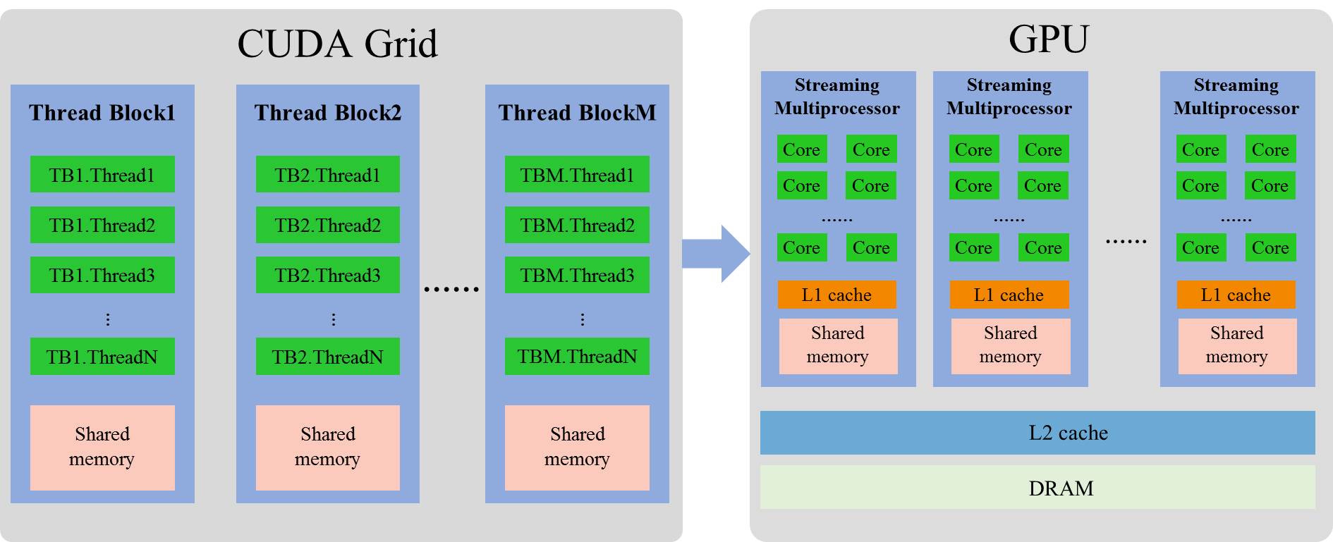
Figure 1: Thread Batching and GPU architecture. The computations are executed using a batch of threads organized as a grid of thread blocks, which are allocated to streaming multiprocessors on GPU.

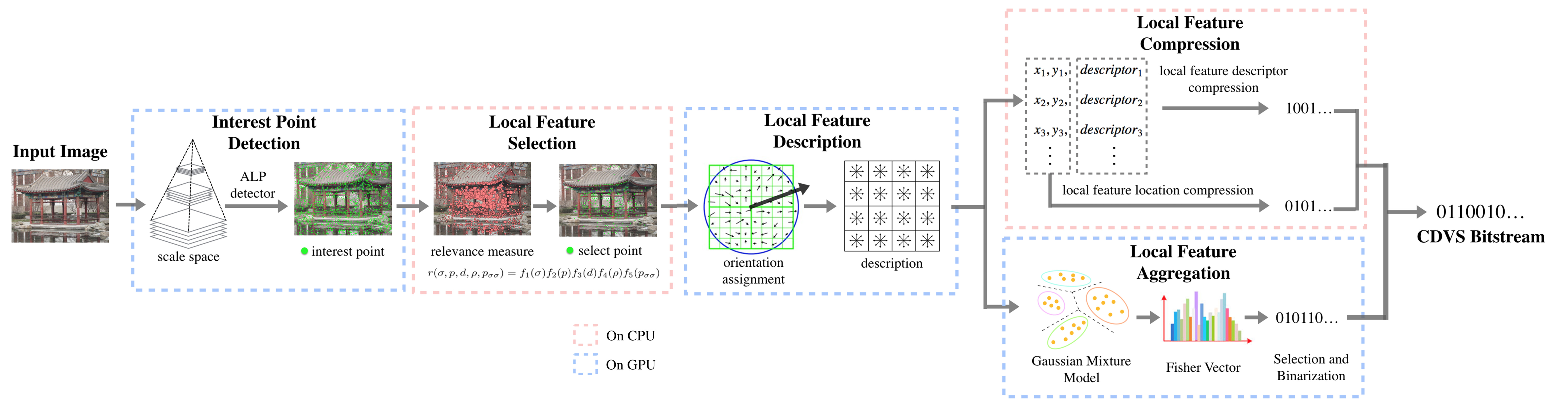
Figure 2: The normative blocks of the CDVS standard implemented on GPU-CPU hybrid computing architecture.

II-B Review of GPU based feature extraction

Based on the outstanding parallel performance of GPU, there has been a fast growing interest in applying GPU to speed up visual feature descriptor construction. Especially, tremendous algorithms have been proposed for GPU based SIFT implementation [11, 12, 13, 14, 15, 16, 17], as SIFT descriptors require high computational cost and huge demand of memory. In [11], an efficient GPU implementation of SIFT was presented based on the vector operations of GPU by texture packing, and 20 fps with the QuadroxFX 3400 GPU was realized. In [12], an open source GPU/CPU mix implementation for SIFT was provided and achieved 27.1 fps with CUDA on 8800GTX GPU. In [15], with GTX 1060 GPU the CUDA-SIFT implementation consumes 2.7 ms for the images with resolution $1280\times 960$ and 3.8 ms for the resolution $1920\times 1080$. Wang et al. further analyzed the workload of SIFT in [16] and proposed to distribute the feature extraction tasks to CPU and GPU, such that a speed of 10 fps for a $320\times 256$ image and 41% energy consumption reduction can be achieved. Besides SIFT, the speeded-up robust feature (SURF) [3, 18] and fisher vectors (FV) [19] were also explored in implementing using GPU platform, and around an order of magnitude speedup was achieved compared to CPU based implementation.

Besides hand-crafted features, recently convolutional neural network based features have achieved promising performance in various computer vision tasks such as image classification [20] and retrieval [21]. CNN requires extremely fast parallel feature extraction on GPU. In [20], a highly optimized GPU implementation of CNN is made publicly available for training networks. A number of CNN softwares based on CUDA using NVIDIA GPUs have also been developed, such as Caffe [22] and TensorFlow [23].

However, although there are many visual feature descriptors implemented on GPU, they are inferior in fulfilling several practical but crucial requirements, e.g., low bandwidth cost, high performance, good compactness, and the excessive GPU resource consumption. Therefore, the very fast and standard compliant CDVS encoder over GPU platforms can elegantly contribute to the state-of-the-art large-scale visual search.

III CDVS Revisit for Speedup

Targeting high accuracy and low bandwidth, CDVS has achieved significant success. Although several technique proposals [24, 25, 26, 27, 28, 8] were proposed to speed up the encoding process of CDVS, it cannot fulfill real-time requirement on CPU platform. To reduce the computational complexity, CDVS first downsamples the input images into low resolution with the longer side less than 640. However, CDVS extraction still needs more than 100 ms for one image [8].

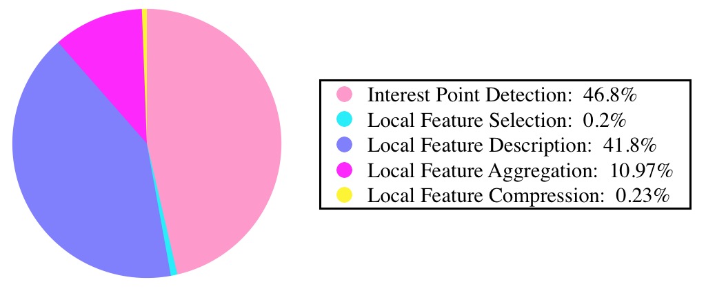
Figure 3: The running time consumption for different modules of CDVS, tested on Linux PC with Intel(R) Xeon(R) CPU E5-2650 v2@2.60GHz.

As illustrated in Fig.2, the CDVS encoder can be divided into five major modules, i.e., interest point detection, local feature selection, description, compression and aggregation. To analyze the computation cost of different modules, we test the running time of each module using TM14.0 on 1000 images with resolution $640\times 480$. Fig.3 shows the percentage of average running time for different modules. From the results we can see that interest point detection, local feature description and aggregation take up most of the running time, more than 99.5%. Therefore, the optimization strategy of CDVS encoders are centralized in the three modules.

III-A Interest Point Detection

The interest point detection consists of two stages, i.e., scale-space construction and extremum detection. The CDVS constructs the scale space as an image pyramid which is generated by filtering the input image via a series of 2D separable Gaussian filters at increasing scale factors. The interest points are regarded as the scale-space extrema of the normalized derivatives of each scale in an image pyramid, which is generated by applying Laplacian filter to each scale image. Therefore, there are multiple convolution operations for input image $I$ with different scale factors as follows,

$$L_{k}=I*g_{k}*f,$$ (1)

where $g_{k}$ and $f$ are the Gaussian and Laplacian kernels, respectively. Obviously, it is a computation intensive process.

To speed up the process of LoG filtering, the Block based Frequency Domain Laplacian of Gaussian (BFLoG) filtering [24, 25, 26, 8] is proposed instead of that in spatial domain. The original input image is first decomposed into overlapped blocks, which are further transformed into frequency domain using Discrete Fourier Transform (DFT). Then, the spatial domain convolution operation can be equivalently implemented by element-wise product between the frequency image matrix and frequency filter kernel matrix. To remove the FFTs for filter kernels, BFLoG adopts the fixed block size to pre-compute convolution kernels in DFT domain, and the pre-computation also reduces the memory cost. Due to Fast Fourier Transform (FFT) [29], the computational complexity of convolution in spatial domain $\mathcal{O}(M^{2}N^{2})$ becomes $\mathcal{O}(4N^{2}logN^{2}-11N^{2}+16N)$, where $M$ and $N$ are the size of square filter and square block. By optimizing the block size and overlap size, the BFLoG achieves about 47% filtering time reduction with ignorable performance variations.

Although the block-level interest point detection are independent of each other, the pixels of each block are dependent in FFT calculation, which makes it difficult to be implemented on pixel-level parallelism. To reduce the boundary effects, BFLoG utilizes $R$ overlapped pixels for each $N\times N$ block, which leads to extra computational burdens. Empirically, the block size $N=128$ and overlapped size $R=16$ are optimal for performance and efficiency. However, for an $640\times 480$ image, only 35 blocks can be executed in parallel, which is much fewer than the number of GPU cores.

For the subsequent extremum detection, BFLoG has to recompose the (LoG and Gaussian) filtered representations, which leads to extra IFFT operations and memory increase. There are 8 inverse IFFTs for each block with 5 scales as illustrated in Fig.4. Considering the Laplacian filter kernel with fixed and small size for all the scale images, the computational cost of Laplacian convolution is much lower than that of Gaussian convolution. Therefore, Duan et al. proposed the mixture domain LoG filtering approach (BMLoG) to further reduce the computation cost of BFLoG by applying Gaussian convolution in frequency domain and Laplacian convolution in spatial domain as shown in Fig.4. As a result, the filtering process has 1 FFT and 5 IFFT operations plus $5\times 7$ adds/subtractions of each pixel for the Laplacian convolution, which achieves about 20% filtering time reduction [27].

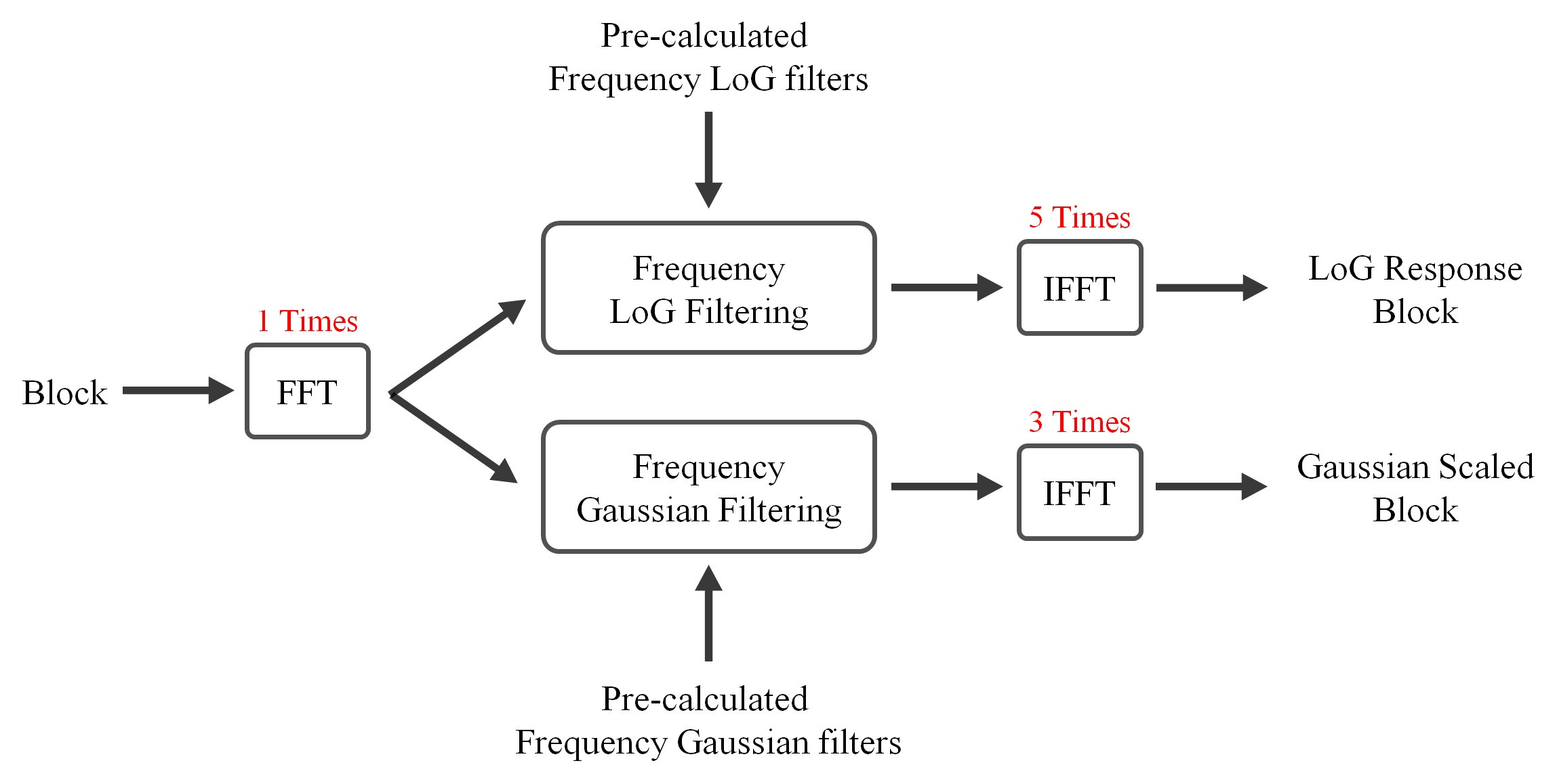
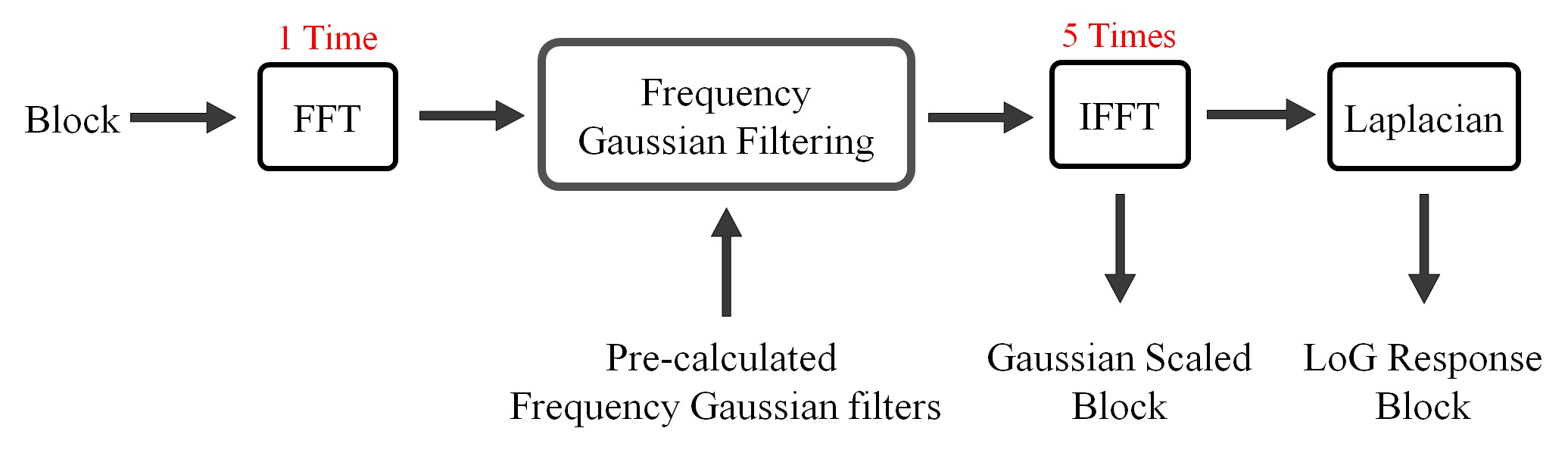
Figure 4: The filtering approach for BFLoG and BMLoG, (a) BFLoG, (b) BMLoG.

After the LoG filtering, interest points are detected by identifying the local extrema, which needs to compare each sample point with its 8 neighbors in the current scale image and 18 neighbors in the above and below scales. CDVS adopts an alternative extrema detection algorithm with low computational complexity, which is a low-degree polynomial (ALP) approach [28]. By assuming that LoG kernel can be approximated by linear combinations of LoG kernels at different coordinates and scales, ALP approximates the LoG scale space by a third-degree polynomial of the scale $\sigma_{k}$ for each sample point $(x,y)$,

$$p(x,y,\sigma_{k})=\sum_{i=0}^{3}\alpha_{i}(x,y)\sigma_{k}^{i},$$ (2)

where the polynomial coefficients are functions of the image coordinates $(x,y)$,

$$\alpha_{i}=\sum_{k=0}^{K-1}\beta_{k,i}L_{k}(x,y),~{}~{}i=0,1,2,3.$$ (3)

The parameters, $\{\beta_{k,i}\}$, correspond to the $K$ predefined scales $\sigma_{k}$ and $\{L_{k}|k=0,\cdots,K\}$ are the LoG filtered images in one octave. ALP first finds the scales of the extrema via the derivatives with respect to $\sigma_{k}$ of the polynomial in Eqn.(2), and then it compares the point with its 8 neighbors. Compared with the previous methods, ALP is more efficient by reducing the 18 comparisons for each sample point to 8 comparisons.

Although these fast algorithms significantly reduce both the computational and memory costs, the computational burden of interest point detection is still too high for CPU, and the interest point detection is still the most time-consuming module. Fortunately, the calculations of convolution and ALP are suitable for pixel-level parallelism. These computations can well fit into highly parallel architectures like GPU.

III-B Local Feature selection and Description

Since there are usually hundreds or thousands of interest points in an image as illustrated in Fig. 6, it brings difficulties in compact representation and low computational cost when processing all features. Fig. 5 shows the relationship between computational cost and feature number. Selecting a subset of good features may save considerable computation time for the subsequent local feature description, compression and aggregation. Therefore, the core module of local feature selection plays an important role in reducing the computational cost.

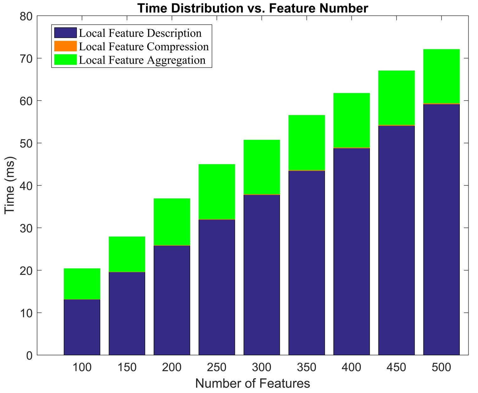
Figure 5: The time consumption of CDVS modules without local feature selection when extracting different number of local features. The test is performed on Linux PC with Intel(R) Xeon(R) CPU E5-2650 v2@2.60GHz for 1000 images with resolution $640\times 480$.

During the development of CDVS, lots of methods [30, 31, 32] are proposed to describe and compress a subset of essential interest points while maintaining and even improving search accuracy. The basic rationale is based on the statistical characteristics to select the interest points with high probability being positive matching ones and remove the noise points. Samsung Electronic proposed to extract features in visual attention regions [30] based on the assumption that more relevant descriptors are located in salient regions for human visual system. Thus, computation overhead can be significantly reduced by applying feature extraction to regions of interest (ROI). However, this method leads to performance loss due to the inconsistency between ROIs and the distribution of true matching points. Moreover, it is difficult to define accurate ROIs at low computational cost.

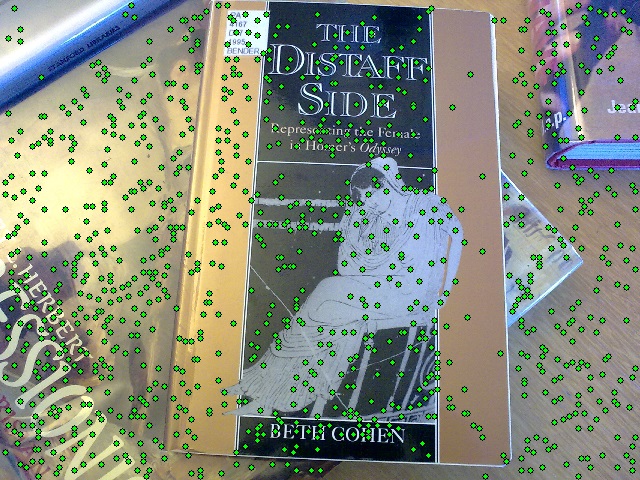
(a) Interest points in query image

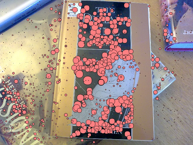
(b) Relevance of the interest points

Figure 6: Comparison of ALP interest point distribution and the selected interest point distribution using the ranked values in Eqn.(5), (a) ALP interest points, (b) relevance of the interest points, where the circle size of interest points are proportional to the relevance measure.

Finally, CDVS adopts a relevance measure to evaluate feature significance in image matching and retrieval performance based on five statistical characteristics of interest points, including the scale $\sigma$ of the interest point, the scale-normalized LoG response value $p$ obtained with $p(x,y,\sigma)$ as in Eqn.(2), the distance $d$ from the interest point to the image center, the ratio $\rho$ of the squared trace of Hessian to the determinant of the Hessian, and the second derivative $p_{\sigma\sigma}$ of the scale space function with regard to $\sigma$, i.e., $\frac{\partial^{2}p(x,y,\sigma)}{\partial^{2}\sigma}$. The relevance measure indicates the priori probability of a query feature correctly matching a feature of database images. Given a characteristic parameter by symbol $y$ lying within region $B$, the conditional probability for correct matching is

$$f(c=1|y\in B)=\frac{P(y\in B,c=1)}{P(y\in B)}.$$ (4)

CDVS attempted to learn these conditional distributions over training pairwise feature matching from a large database of matching image pairs[32], and stored the quantized characteristic parameters and their corresponding function values of conditional distributions in normative tables, which may minimize the computational cost by look-up tables.

By assuming independency of the characteristic parameters, the relevant score for each point is obtained by multiplying these conditional probabilities:

$$r(\sigma,p,d,\rho,p_{\sigma\sigma})=f_{1}(\sigma)f_{2}(p)f_{3}(d)f_{4}(\rho)f_{5}(p_{\sigma\sigma}).$$ (5)

Therefore, a subset of $N$ interest points will be selected by ranking relevance measure $r$, and the feature description is only performed on the selected points. Fig.6 shows the distribution comparison before and after selecting salient interest points. The circle size of interest points in Fig.6(b) are proportional to the relevance value. We can see that the selected relevant interest points by Eqn.(5) basically fall into the salient regions, in which feature selection can significantly reduce the computational cost without performance degeneration. To balance the computational cost and search accuracy, CDVS empirically selects around 300 local feature descriptors to represent an image, which saves more than 30% computational cost (seeing Fig.5).

III-C Local Feature Compression

The uncompressed SIFT descriptors are difficult to use in practice for two reasons, 1) size limitation: it needs 1024 bits for each descriptor by representing each dimension with 1 byte; 2) speed limitation: the computational cost for byte-vector distance is too high over large-scale databases. Therefore, the local feature compression and fast matching in compressed domain are necessary.

During CDVS development, two kinds of compression algorithms based on vector quantization and transform are widely discussed and both of them achieve significant improvement on compression performance and computational efficiency. In early stage of CDVS, the Test Model under Consideration (TMuC) for CDVS [33] employed tree structured vector quantization (TSVQ) [34] and product quantization (PQ) [35] to make compact descriptors. However, these methods need to store huge codebooks, thereby leading to heavy computational burdens. For example, in [36], the authors proposed PQ-SIFT to quantize local descriptors with over a large vocabulary with 1 million centroids for 16 sub-segments.

The Multi-Stage Vector Quantization (MSVQ) scheme [37] was adopted into the test model TM2.0 and significantly reduced the size of quantization tables. The MSVQ quantization consists of two stages, i.e., Tree Structured Vector Quantization (TSVQ) for the original raw descriptors at the 1st stage and the subsequent Product Quantization (PQ) for the residuals at the 2nd stage. After training the MSVQ over 6 million SIFT descriptors, the MSVQ only utilizes a 2-level tree-structure quantization table with 2048 visual centers and a PQ table with $\sim$16K centers. Therefore, in total comparison operations are reduced to 256 (1st level TSVQ)+8 (2nd level TSVQ)+16K (PQ) for each descriptor, which significantly reduces the computational cost in searching codewords.

To further reduce the computational cost, CDVS finally adopts the transform coding with scalar quantization instead of the MSVQ. For each SIFT subregion Histogram of Gradients (HoG) $\bm{h}$ with bins {$h_{0}\cdots h_{7}$}, CDVS applies an order-8 linear transform to capture the shape of HoGs. To improve the discriminative power of descriptors, CDVS defines two sets of transforms and applies different transforms to neighboring subregion HoGs, and the transforms are implemented via addtion/subtraction and shift operations with extremely low complexity. Each element of the transformed descriptors is further individually quantized to three values, $-1$, $0$ and $+1$, using quantization thresholds calculated from the off-line learned probability density function of that element. This transform coding method exhibits much lower computational cost than MSVQ while keeping comparable performance. More importantly, the transform coding method is codebook free, and it is more suitable for GPU since the I/O speed is actually the bottleneck of GPU in large-scale computing.

III-D Local Feature Aggregation

The global descriptors with highly efficient distance computation are crucial for fast large-scale visual search. Different global descriptors were proposed in CDVS development such as Residual Enhanced Visual Vector (REVV)[38, 39], Robust Visual Descriptor (RVD)[40, 41] and Scalable Compressed Fisher Vector (SCFV)[42, 43]. The REVV utilizes a set of 190 centroids from k-means clustering of SIFT descriptors off-line, and assigns each uncompressed SIFT descriptor of an input image to its nearest centroid in terms of L2 distance. The difference or residual between each SIFT descriptor and its nearest centroid is computed, and the mean residual of all the SIFT descriptors quantized to the same centroid is computed for a centroid. A power law with exponent value 0.6 is applied. With dimension reduction via PCA, these residual vectors are binarized according to its sign and concatenated to form a global descriptor. Although the REVV is with very low computational cost and memory footprint, the performance is yet to be improved.

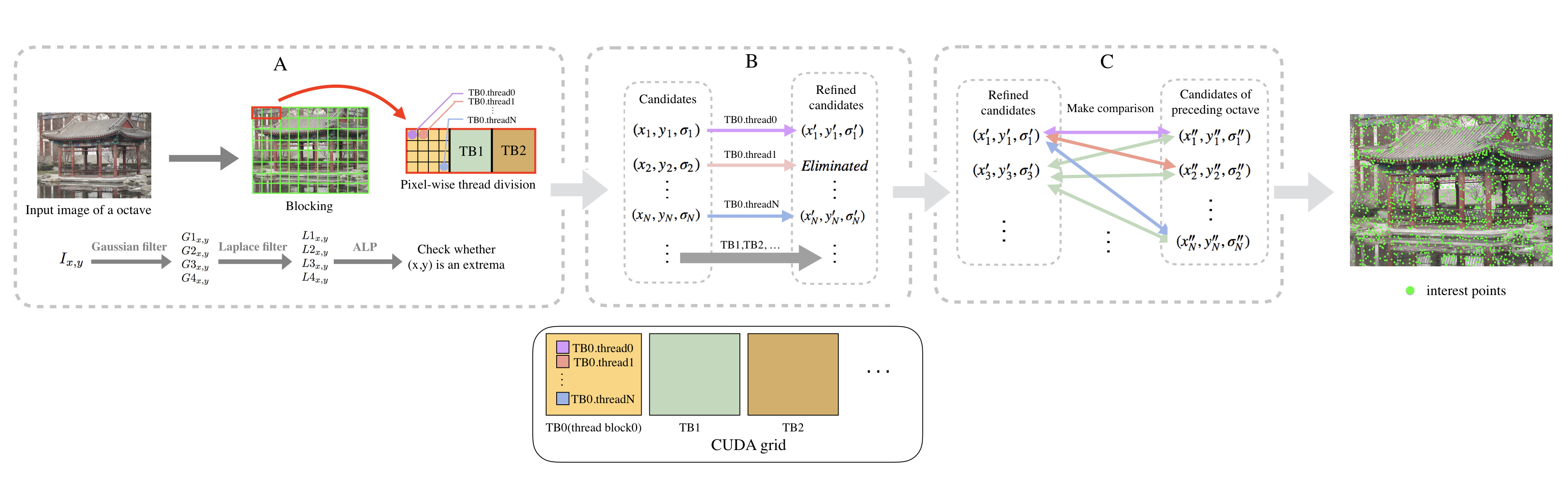
Figure 7: The block diagram of the interest point detection implementation on GPU

Bober et al. proposed an enhanced global descriptor, RVD, which improves the robustness of REVV by assigning each SIFT descriptor to multiple cetroids while reducing the computational cost. To reduce the computational cost, the RVD shifts the PCA to the first stage to reduce the computational cost for the subsequent calculations, and utilizes the matrix multiplication to implement PCA. This transform reduces the PCA computational complexity from $\mathcal{O}(n^{2})$ to $\mathcal{O}(n)$, where $n$ is the number of local features. In addition, the matrix operations has been well implemented and optimized on GPU by NVIDIA, i.e., cuBLAS, and can greatly reduce the global memory operations compared with non-matrix operations. Furthermore, the RVD utilizes the L1 norm distance between SIFT descriptors and centroids instead of L2 norm distance in REVV to avoid the computation-intensive multiplication operations. Although each of the SIFT descriptors is assigned to multiple centroids with a bit increased computation, the RVD achieves better performance compared with REVV.

Finally, the CDVS adopted the SCFV as its global descriptor, which takes a Gaussian Mixture Model (GMM) with 512 components to capture the distribution of up to $N$ selected local feature descriptors. The SCFV also firstly reduces the SIFT dimensions utilizing PCA matrix, but it transforms the 128D SIFT into 32D instead of 48D of RVD, which further reduces the computational cost for subsequent operations. For each 32D vector $x_{t}$, the major computation in SCFV include probability in Eqn.(6), the accumulated gradient vector $g_{\mu_{i}}^{x}$ with respect to the mean of the $i^{th}$ Gaussian function in Eqn.(7), and its standard deviation $\delta(i)$ in Eqn.(8),

$$\gamma_{t}(i)=\frac{w_{i}p_{i}(x_{t}|\lambda)}{\sum_{j=0}^{N}w_{j}p_{j}(x_{t}|\lambda)},$$ (6)

$$g_{\mu_{i}}^{x}=\frac{1}{K\sqrt{w_{i}}}\sum_{t=0}^{K-1}\gamma_{t}(i)\frac{x_{t}-\mu_{i}}{\sigma_{i}},$$ (7)

$$\delta(i)=\sqrt{\frac{1}{32}\sum_{j=0}^{31}(g_{j}-\frac{1}{32}\sum_{k=0}^{31}g_{k})^{2}},$$ (8)

where $p_{i}(x_{t}|\lambda)$ is the Gaussian function, $w_{i}$ is the weight of the $i^{th}$ Gaussian function, and $N$ is the number of local features. Then, the Gaussian components are ranked in descending order according to $\delta$, and the top $K$ ones are selected based on the bit budget. Since only 250 local feature and 512 Gaussian functions are applied in CDVS, there are around 4.5 million multiplications/divisions for these 32D features, which is more than that in RVD, about 36 thousands multiplicaitons/divisions. However, the SCFV achieves very promising search performance and fulfills novel bit rate scalability, and moreover all these calculations can be transformed into matrix operations, which can be well implemented and optimized in parallel on GPU achieving significant speedup. The detailed speedup results for SCFV on GPU are shown in Fig.15(c).

IV Fast CDVS Encoder using GPU-CPU Hybrid Computing

Although great efforts have been made to reduce the computational complexity of CDVS, it is still difficult to implement highly efficient CDVS on CPU even with multiple threads in parallel. By leveraging the massive parallel process cores of GPU, we design and implement the very fast CDVS encoder using GPU-CPU hybrid computing. Three major time-consuming modules, i.e., interest point detection, local feature description and aggregation, are shifted to GPU platform, while the others remains on CPU platform as shown in Fig.2. In addition, the local feature compression and aggregation are independent process, they can be in parallel performed on CPU and GPU simultaneously, which elegantly leverages the computational resources on CPU and GPU. In the following subsection, we present technical details on interest point detection, local feature description and aggregation.

IV-A Interest Point Detection on GPU

In interest point detection, we adopt sperate Gaussian filters to construct the image pyramid, utilize Laplacian filter and ALP to detect interest points. Distinct from BFLoG, the spatial domain Gaussian and Laplacian filtering can be implemented in much higher degree of parallelism with very low memory usage, while the BFLoG is only implemented on block-level parallel with doubling memory usage due to the complex operations in FFT. In addition, the spatial domain filtering can be completed in one step, while the BFLoG need three sequential steps, i.e., FFT, element-wise production and IFFT, which incurs more process time for GPU.

The implementation of interest point detection comprises of three basic stages as illustrated in Fig.7. Part A illustrates the implementation of LoG filtering and ALP detection, which outputs the interest point candidates. To achieve high degree parallelism, the input image is first divided into $N\times N$ blocks, and each block is assigned to a thread block (TB) to perform LoG filtering. Since the access speed for shared memory is much higher than graphic memory, these image blocks are loaded into the shared memory of their corresponding thread blocks. Then, the threads in the same TB access the pixels from its shared memory sequentially, i.e., TB0.thread0 access the first pixel, TB.thread1 access the second pixel, and so no. This memory access mechanism is to make full use of the merit of global memory coalescing to reduce memory access time cost. Then, the Gaussian filtering, Laplacian filtering and ALP detector are sequentially performed in corresponding threads. In our implementation, we specify that both image block and thread block are of the same size, in which each pixel is processed on each thread in parallel.

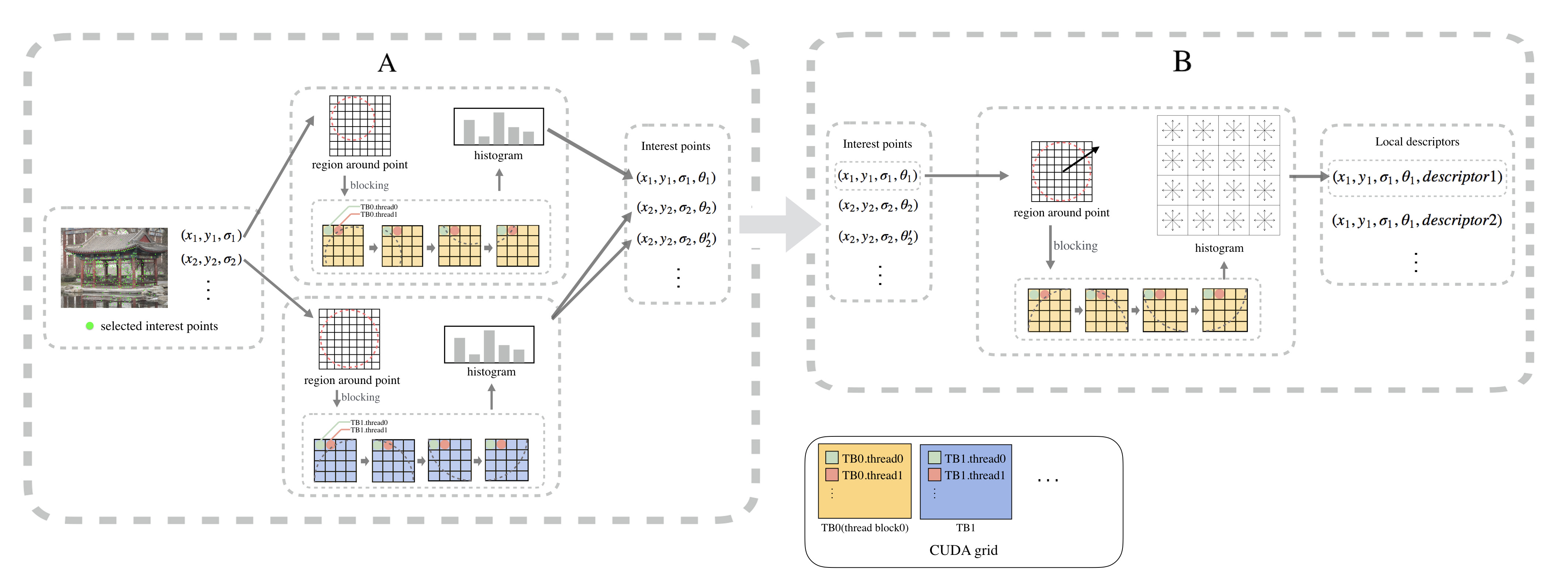
Figure 8: The block diagram of the local feature description implementation on GPU

For Part B, the interest point candidates are refined to remove unstable interest points and more accurate locations of interest points are determined. To speed up the process, we reorganize the interest point data $(x_{i},y_{i},\sigma_{i})$ and the corresponding pixels in its $3\times 3$ neighborhood into a continuous queue. For $N$ continuous candidates, we assign a TB with $N$ threads to calculate the LoG response in a $3\times 3$ region around the candidate, which employs the global memory coalescing to speed up the process. Afterwards, the interest points considered as an unstable ones are removed out, otherwise, more accurate position are updated by the interpolation.

In Part C, the final interest points are determined by comparing the neighboring ones in adjacent octaves. Likewise, we first construct two queues for the interest point candidates in current octave and preceding octave respectively, and then apply one TB to perform the comparisons between one candidate in current octave and all the candidates in preceding octave by the global memory coalescing. Each thread first executes the comparison between two candidates. If they are close enough in $(x,y,\sigma)$ space, the candidate with lower LoG response is eliminated. The implementation details on each thread are illustrated in Algorithm 1 using pseudo-code.

Algorithm 1 Interest Point Detection on GPU

1:Input image $I$, $G_{0,0}=I$

2:A queue of interest points

3:for $o$ = 0 to $num\_octave$ do

4:     //Stage A: Scale-space for $G_{o,0}$

5:     Load $G_{o,0}$ to shared memory

6:     parfor each pixel($i$,$j$) do

7:         //A thread corresponds to a pixel

8:         $T_{k}[i][j]$ = $\sum_{p=-r_{k}}^{r_{k}}G_{o,0}[i+p][j]*g_{k}[p]$

9:         $G_{o,k}[i][j]$ = $\sum_{p=-r_{k}}^{r_{k}}T_{k}[i][j+p]*g_{k}[p]$

10:         $L_{o,k}[i][j]=\sum_{m,n=-1}^{1}G_{o,k}[i+m][j+n]*f[m][n]$

11:         Local extremum determination via Eqn.(2)

12:     end parfor

13:     //Stage B: Refine extremum location

14:     parfor each candidate $(x_{o},y_{o},\sigma_{o})$ in $Q_{o}$ do

15:         //A thread corresponds to a candidate

16:         $(x^{\prime}_{o},y^{\prime}_{o},\sigma^{\prime}_{o})$ = CoordinateRefine$(x_{o},y_{o},\sigma_{o})$

17:     end parfor

18:     //Stage C: Extremum determination between octaves

19:     parfor  a pair candidates  do

20:         //A thread corresponds to a pair

21:         $dis$ = distance($(x^{\prime}_{o},y^{\prime}_{o},\sigma_{o})$,$(x^{\prime}_{o-1},y^{\prime}_{o-1},\sigma^{\prime}_{o-1})$)

22:         Update $Q_{o}$ and $Q_{o-1}$ according $dis$ and $p(x^{\prime}_{o},y^{\prime}_{o},\sigma^{\prime}_{o})$, $p(x^{\prime}_{o-1},y^{\prime}_{o-1},\sigma^{\prime}_{o-1})$

23:     end parfor

24:     Merge $Q_{o}$ into output

25:     Downsampling $G_{o,4}$ to $G_{o+1,0}$

26:end for

The pixel-level thread allocation and efficient shared memory assess significantly reduce runtime cost for interest point detection. Based on our experimental results, the optimal GPU implementation can achieve around 26 times speedup compared with that on CPU platform, and the running time decrease from 56.2ms to 2.16ms for $640\times 480$ images.

IV-B Local Feature Description on GPU

The local feature description includes two stages, i.e., orientation computation and SIFT description. To allow rotation invariance for local feature descriptors, each interest point is assigned one or more dominant orientations based on the distribution of the quantized gradient directions in its neighborhood with radius $3.96\sigma$. To derive the dominant orientation, an orientation histogram with 36 bins shall be formed from the computed gradient orientations. The orientations with bin values greater than 0.8 times of the highest peak are kept as orientations of the interest point. For SIFT description, the image patch centered at interest point $(x,y)$ is first rotated to the angle of its orientation, and then it is divided into 4 horizontal and 4 vertical spatial subregions referred to as cells. The size of each side of each cell shall be $3\sigma$ pixels. From each cell, a histogram of gradients with 8 orientation bins, referred to as cell histogram, is generated. The SIFT descriptor is formed by concatenating these cell histograms.

Based on the above introduction, the local feature description is divided into two stages as illustrated in Fig.8. The histogram construction occupies major computation. To maximize the degree of parallelism, we assign one TB to each interest point to generate the orientation histogram and compute the dominant orientations. However, the pixel-level parallelism with global memory coalescing is difficult to implement by simply allocating one thread to compute the gradient of each pixel and sum them up into a histogram. This is because that the number of threads in one TB should be the same, while the image patch size $3.96\sigma$ is variant for different interest points. If we allocate threads according to the largest image patch, the amount of pixels is much more than the available threads in one TB.

Algorithm 2 Local Feature Description on GPU

1:Interest points after feature seletction

2:The descriptors of interest points

3://Stage A: orientation assignment

4:parfor each interest point $(x_{ctr},y_{ctr},\sigma)$  do

5:     //Apply a thread block to an interest point

6:     Load $R\times R$ regions in shared memory

7:     parfor each $(x,y)$ in $R\times R$ do

8:         //a thread corresponds to a pixel

9:         if distance$((x_{ctr},y_{ctr})$,$(x,y))<3.96\sigma$  then

10:              Add gradient magnitudes and orientations to histogram

11:         end if

12:         Compute the orientation from the histogram

13:     end parfor

14:end parfor

15://Stage B: Feature description

16:parfor Each interest point $(x_{ctr},y_{ctr},\sigma,\theta)$  do

17:     //Apply a thread block to an interest point

18:     parfor each $(x,y)$ in $R\times R$ do

19:         //a thread corresponds to a pixel

20:         if distance$((x_{ctr},y_{ctr})$,$(x,y))<6\sigma$  then

21:              Add gradient magnitudes and orientations to histogram

22:         end if

23:     end parfor

24:     Generate the 128D descriptor from the histogram

25:end parfor

To solve the problem of variant patch size, we design a novel block-based pixel-level parallelization method. For each image patch, we divide it into non-overlapped $N\times N$ sub-patches, and allocate each TB with $N\times N$ threads. Then, the gradient computation can be performed in pixel-level parallelism, and gradients are then exported to shared memory to form gradient histograms by atomic addition. The detailed design for local feature description is illustrated via pseudocode in Algorithm 2. Compared with the feature-level parallelization which assigns one independent thread to each interest point, the proposed block-based pixel-level parallelization is more efficient. Because feature-wise parallelization would lead to very unbalanced workload among threads and thus degenerate the processing efficiency on GPU due to variant patch sizes for interest points. Besides, local feature selection is applied in CDVS to keep less than $N$ ($N$ is usually smaller than 650) features for describing an image. It means that at most $N$ threads can be launched simultaneously for feature-wise parallelization, which incurs much less than cores in GPU. Our GPU implementation for local feature description achieves more than 90 times speedup compared that on CPU at different bitrates, the running time significantly decreases from $33.2\sim 79.2$ ms to $0.4\sim 0.83$ ms.

IV-C Local Feature Aggregation on GPU

When the stages of interest point detection and local feature description have been implemented optimally, the proportion of time-consumption for local feature aggregation increase from 10% up to 80%, which becomes the bottleneck in the whole pipeline of CDVS encoding. Hence, the remaining issue is to speed up the local feature aggregation. As introduced in Section III-D, there are two parts, i) dimension reduction via PCA, ii) the fisher vector aggregation. The PCA calculation in CDVS is defined by matrix multiplication, which can be well fulfilled by calling the highly optimized matrix operation lib in CUDA.

To speed up the fisher vector aggregation, we first transform the probability calculation for each 32D local descriptors in Eq.(9) into the matrix multiplications and a set of element-wise operations as shown in Egn.(10).

$$P_{i,j}=\sum_{k=0}^{31}\frac{(D_{i,k}-M_{j,k})^{2}}{V_{j,k}},$$ (9)

$$P=(D.*D)*(1./V^{T})-2D*(M./V)^{T}+O*((M.*M)./V)^{T}.$$ (10)

Here, $P_{i,j}$ represents the probability of the $i^{th}$ descriptor under the $j^{th}$ GMM component, $D_{i,k}$ denotes the $k^{th}$ dimension of the $i^{th}$ descriptor, $M_{j,k}$ and $V_{j,k}$ denote the $k^{th}$ dimension of mean and covariance vector for the $j^{th}$ GMM component, O is a matrix filled by 1 and has the same dimension with $D$. The notations, ’.*’ and ’./’ represent the element-wise multiplication and division. These matrix operations can be efficiently performed by calling the well optimized matrix operation library in CUDA. Similarly, we derive the matrix implementation for the calculation of accumulated gradient vectors with respect to the mean and variance denoted as $(GM)$ and $(GV)$, the calculations of which are transformed from Eqn.(11) and Eqn.(13) to Eqn.(12) and Eqn.(14).

$$GM_{i,j}=\sum_{k=0}^{DescNum}(\frac{D_{i,k}-M_{j,k}}{V_{j,k}}*Q_{i,j}),$$ (11)

$$GM=(Q^{T}*D-Q^{T}*O.*M)./V,$$ (12)

$$GV_{i,j}=\sum_{i,j}^{DescNum}((\frac{D_{i,k}-M{j,k}}{V_{j,k}})^{2}-1)*Q_{i,j},$$ (13)

$$GV =(Q^{T}*(D.*D)-Q^{T}*D.*2M$$ (14)

$$+Q^{T}*O.*(M.*M-V.*V))./(V.*V).$$

Here $Q$ is the normalized probability of $P$, and $DescNum$ is the number of the local feature descriptors. After these conversions, local feature aggregation module can be implemented by invoking the matrix lib in CUDA, which is well optimized by NVIDIA. Based on the experimental results, the running time of local feature aggregation decreases from around 13 ms to 0.25 ms, and the speedup of GPU implementation is more than 49 times compared that on CPU.

V Experimental Results and Analysis

V-A Databases and Evaluation Criteria

To analyze the performance of the fast CDVS encoder, we perform pairwise matching and image retrieval tasks on patch-level and image-level databases. Two image-level databases are utilized in our experiments, 1) MPEG-CDVS benchmark database [44], which consists of 5 classes: graphics, paintings, video frames, landmarks and common objects; 2) Holiday database [45], which contains images from different scene types to test the robustness to transformations such as rotation, viewpoint, illumination changes and blurring, and is widely used in academic literatures. In addition, we also utilize two patch-level databases, MPEG-CDVS patch database [46] and Winder and Brown database [47], which contain 100K and 500K matching pairs of $64\times 64$ pixels image patches involving canonical scaled and oriented patches.

For performance validation, we adopt the Mean Average Precision (mAP), True Positive Rate (TPR) and False Positive Rate (FPR) to measure the image retrieval and pair matching performance respectively. The mAP for a set of queries is calculated as the mean of the average precision scores for each query, which is defined as follows,

$$mAP=\frac{\sum_{q=1}^{Q}AP(q)}{Q},~{}AP=\int_{0}^{1}\bm{p}(r)dr,$$ (15)

where $Q$ is the number of queries, and $AP$ is the average precision, and $\bm{p}(r)$ is the precision function at recall $r$. The TPR and FPR are calculated as,

$$\emph{TPR}=\frac{\emph{TP}}{\emph{TP}+\emph{FN}},~{}\emph{FPR}=\frac{\emph{FP}}{\emph{FP}+\emph{TN}},$$ (16)

where TP, FP, TN and FN are the number of the true positive, false positive, true negative and false negative retrieval results.

The fast CDVS encoder is implemented based on the latest CDVS reference software TM14.0 using GPU-CPU hybrid computing. In the following section, we validate the improvements of visual search accuracy and descriptor extraction speed, respectively. To fully understand the superior performance of CDVS, we also compare CDVS descriptor with state-of-the-art visual feature descriptors including SIFT [2], SURF [3], ORB [4], BRISK [5], AKAZE [48] and LATCH [49], which are from OpenCV 3.2.0 with default parameters.

V-B Performance Comparison

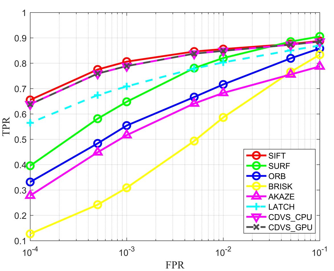
(a) MPEG-CDVS patch database

(b) Winder and Brown patch database

Figure 9: Comparison of ROC curves at patch level for different visual descriptors on (a) MPEG-CDVS database, (b) Winder and Brown database.

In this section, we first show the patch-level evaluation as it provides the initial idea about the performance of descriptors and avoids the influence of different interest point selection strategy. To understand the matching accuracy at different FPR, the ROC curves on MPEG-CDVS and Winder and Brown patch databases are illustrated in Fig.9. The CDVS descriptors generated from CPU and GPU platforms (denoted as CDVS_CPU and CDVS_GPU) yields almost the same pairwise matching results, which verifies that the CDVS encoder is exactly implemented on heterogeneous architectures without performance sacrifice. The patch matching performance of CDVS is only inferior to the original SIFT descriptors, and much more superior to other visual feature descriptors. It is worthy to note, CDVS only needs $32\sim 205$ bits for each descriptor under different rate configurations, and its bitrate is much fewer than that of SIFT, which costs 512 bytes for each descriptor. Although SURF, ORB, BRISK, AKAZE and LATCH are also compact descriptors, their performances are obviously inferior to CDVS and also cannot outperform CDVS in compactness. Herein, there are 256, 128, 256, 244 and 128 bytes in representing each SURF, ORB, BRISK, AKAZE and LATCH descriptor, respectively. In Fig.9, we only utilize 103 bits for each CDVS descriptor.

To verify the overall performance on real images, we carry out image-level evaluation for pair matching and image retrieval tasks. In pairwise matching database, there are 10,155 matching image pairs and 112,175 non-matching in MPEG-CDVS database, and 2072 matching image pairs and 20874 non-matching in Holiday database. Fig. 10 shows the ROC curves on image pair matching task for different visual descriptors. The CDVS descriptors extracted using CPU and GPU platform achieve almost the same performance, and obviously outperform the other competitors. Remarkably, the performance of SIFT descriptors is poor when FPR is low. It is observed that, there are many false matched image pairs where the resulting matched SIFT points are on the background as illustrated in Fig.11. This phenomena verifies that the local feature selection not only reduces the computational cost, but removes the non-meaningful interest points, which significantly contributes to high performance.

In the image retrieval experiments, we compare the performance of the CDVS and its global descriptors generated at 6 pre-defined descriptor lengths: 512 bytes, 1K, 2K, 4K, 8K and 16K in MPEG common test conditions. From the results in Fig.12, we can see that the fast CDVS encoder is well implemented in parallel using GPU platform with negligible performance difference. Table I shows the detailed numerical mAP results for CDVS_CPU and CDVS_GPU respectively, from which the same conclusion can be drawn.

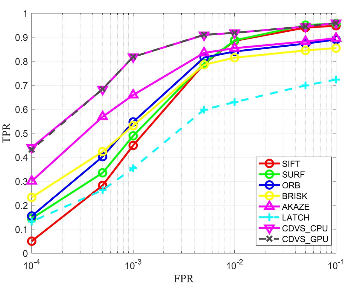
(a) MPEG-CDVS database

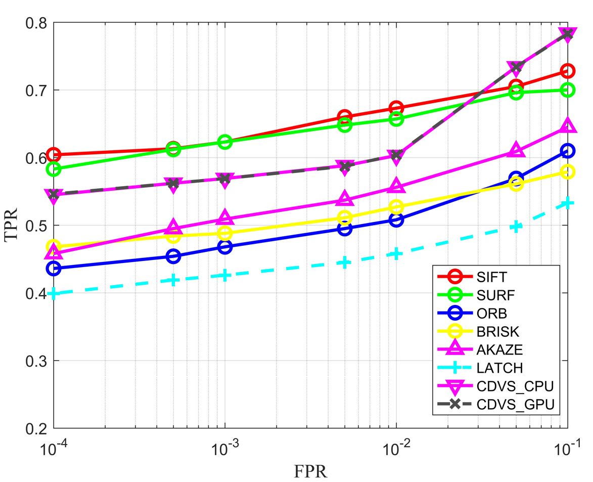
(b) Holiday database

Figure 10: Comparison of ROC curves of image retrieval for different visual feature descriptors on (a) MPEG-CDVS database, (b) Holiday database.

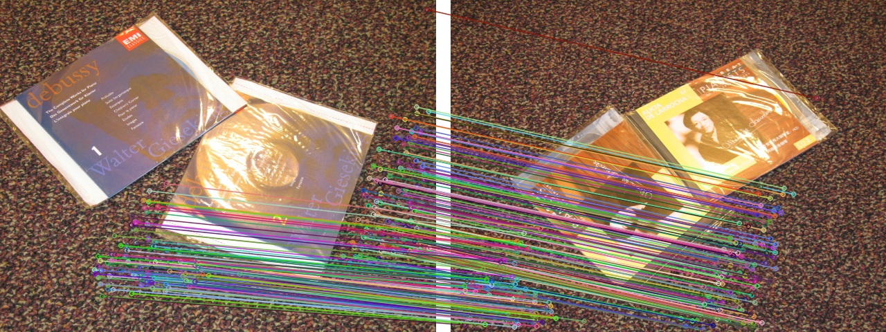
Figure 11: The mismatching example using SIFT descriptors.

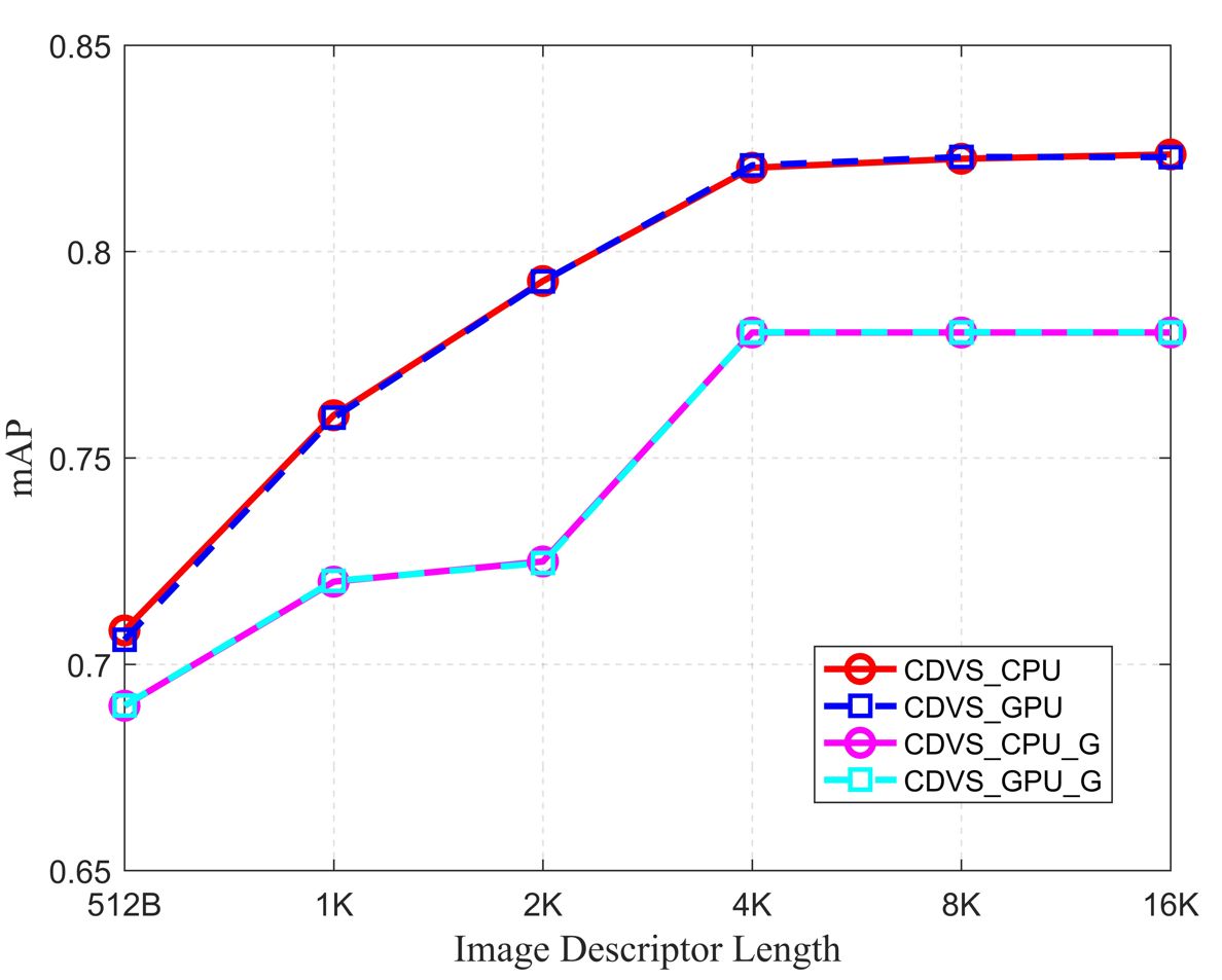
(a) MPEG-CDVS database

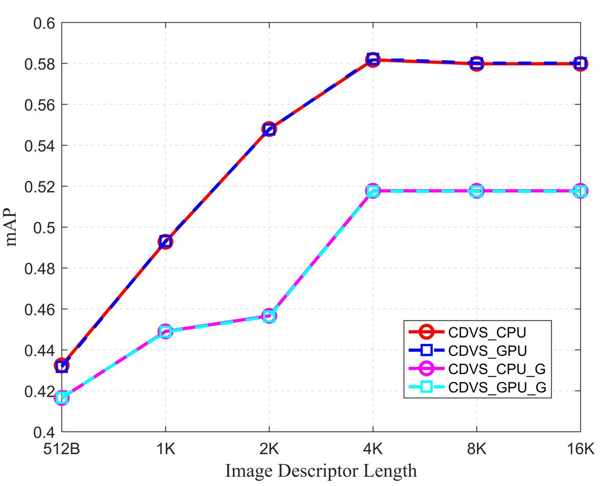
(b) Holiday database

Figure 12: The mAP comparison of image retrieval using CDVS on CPU and GPU platform on (a) MPEG-CDVS database, (b) Holiday database. Herein, CDVS_CPU_G and CDVS_GPU_G represent the CDVS global descriptors generated on CPU and GPU platforms, repspectively.

TABLE I: Comparisons of CDVS CPU and GPU implementations on MPEG-CDVS database (mAP).

	Global		Local+Global
	CPU	GPU	CPU	GPU
512B	0.690	0.690	0.708	0.706
1K	0.720	0.720	0.760	0.760
2K	0.725	0.725	0.793	0.793
4K	0.780	0.781	0.820	0.821
8K	0.780	0.781	0.823	0.823
16K	0.780	0.781	0.824	0.823
Average	0.746	0.746	0.788	0.788

V-C Speed Comparison

In this section, we further show the speedup of the proposed CDVS encoder compared with that on CPU platform. Table II shows the average running time of extracting different visual descriptors on 1000 images with resolution $640\times 480$. The notations CDVS_CPU_L and CDVS_GPU_L represents the running time for CDVS local feature descriptor extraction on CPU and GPU platform. Except for CDVS_GPU and CDVS_GPU_L, all others descriptors are extracted on CPU platform with Intel(R) Xeon(R) CPU E5-2650 v2@2.60GHz. The CDVS_GPU using Quadro GP100 achieves significant speedup compared with that on CPU platform when extracting $200\sim 300$ local features from each image, which achieves more than 35 times speedup for CDVS_CPU. The average of CDVS extraction time is reduced from 116.69 ms on CPU platform to 3.27 ms on GPU platform. Compared with other visual feature descriptors extracted on CPU platform, the proposed CDVS encoder also significantly outperforms them, and it can well satisfy practical real-time applications.

TABLE II: Comparisons of the running time for feature descriptor extraction tested on Linux PC with Intel(R) Xeon(R) CPU E5-2650 v2@2.60GHz and a Quadro GP100 GPU. Unit: ms

Feature	Time	Feature	Time
CDVS_CPU	116.69	SURF	86.27
CDVS_GPU	3.27	ORB	12.6
CDVS_CPU_L	102	BRISK	19.22
CDVS_GPU_L	3.1	AKAZE	135.55
SIFT	368.88	LATCH	159.48

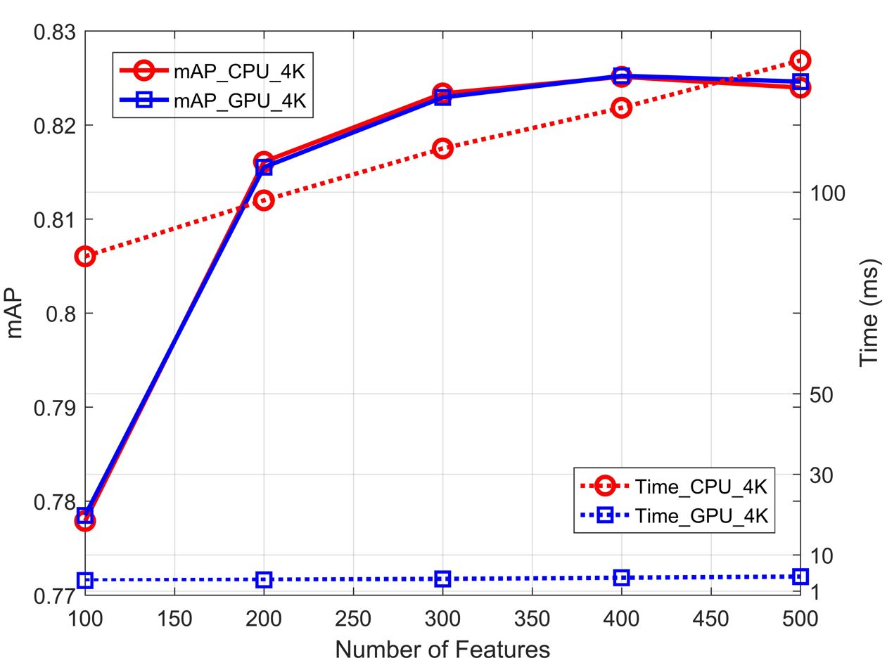
Figure 13: The image retrieval performance vs. extraction time for CDVS on CPU and GPU platform, tested on Linux PC with Intel(R) Xeon(R) CPU E5-2650 v2@2.60GHz and a Quadro GP100 GPU.

Limited by computational power, the CDVS selects no more than 300 local features for each image, which may be less optimal for visual search accuracy especially for high resolution images. Hence, we further analyze the relationship between the number of local features and extraction time (Seeing Fig. 13). We can see that with the increase of local features, the extraction time increases almost linearly on CPU. However, by leveraging GPU, the extraction time cost almost keeps in the same level, about 3 ms. Therefore, more local feature descriptors can be allowed to further improve CDVS performance over GPU platforms, without noticeable increase of computational cost.

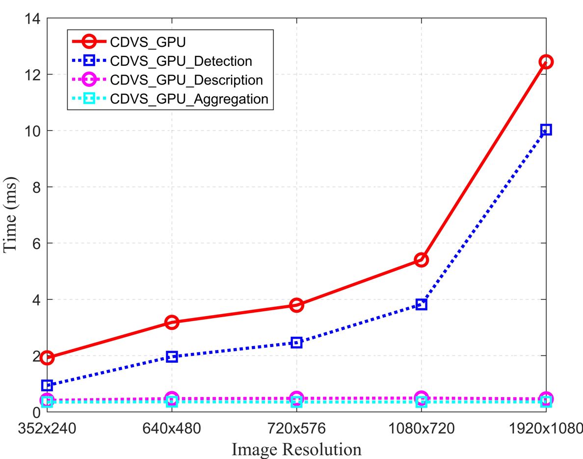
Figure 14: Influences of the resolution on the feature extraction complexity on GPU platform, tested on Linux PC with Intel(R) Xeon(R) CPU E5-2650 v2@2.60GHz and a Quadro GP100 GPU.

When dealing with high resolution images, CDVS needs to first downsample the input images into low resolution with the large side no longer than 640. The downsampling operation can directly reduce the computational cost, but it also brings image distortion or information loss especially for high resolution images. We explore the variations of feature extraction time along with image resolutions for CDVS using GPU platform, and the results are shown in Fig.14. We can see that the most time-consuming module on GPU is still the interest point detection, which has been implemented on pixel-level parallelism. When the pixel number exceeds thread number, the running time will increase significantly. Therefore, the running time increases very slowly when we have enough computational resources on GPU, e.g., the image resolution smaller than $1080\times 720$. The running time for local feature description and aggregation almost does not changes since their computation mainly depend on the number of local features.

To explore the speedup on GPU, we test the running time for these modules on CPU and GPU respectively, and Fig. 15 shows their running time at different pre-defined descriptor length. The CDVS_GPU achieves about 26, 50 and 22 times speedup for interest point detection, local feature description and aggregation compared with that of CDVS_CPU, respectively. Fig.16 shows the running time proportion for different modules with GPU-CPU hybrid computing. We can see that the running time consumption can be covered by the local feature aggregation when using GPU-CPU hybrid computing.

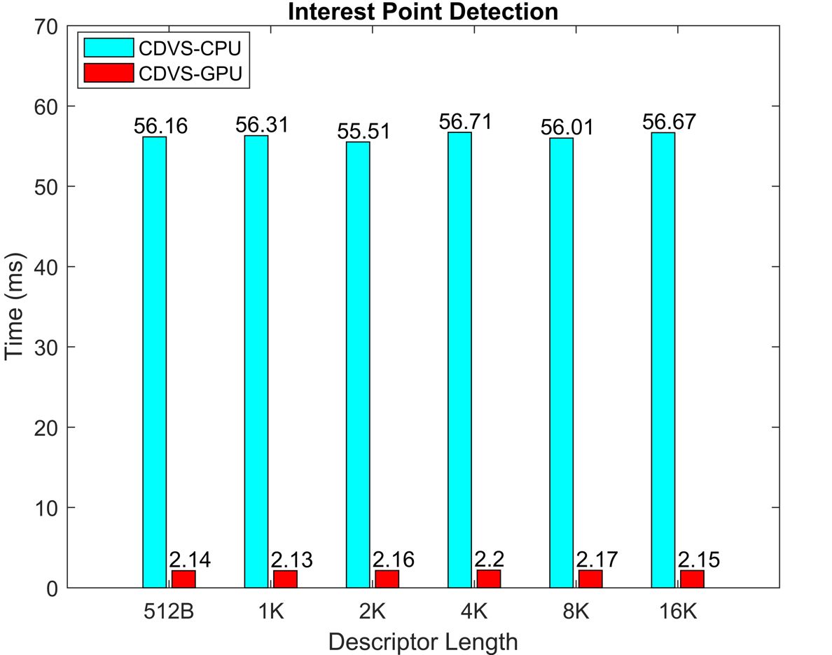
(a)

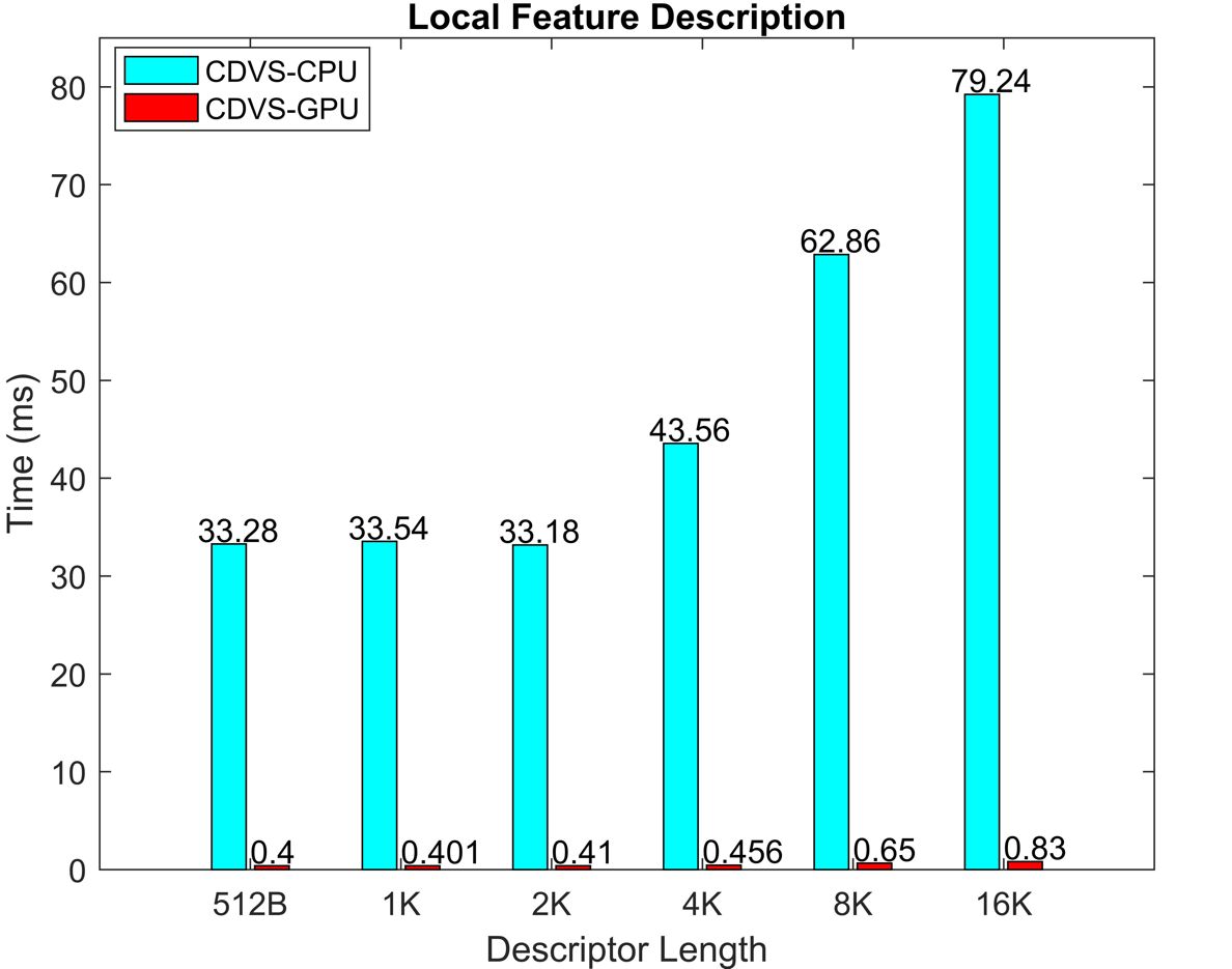
(b)

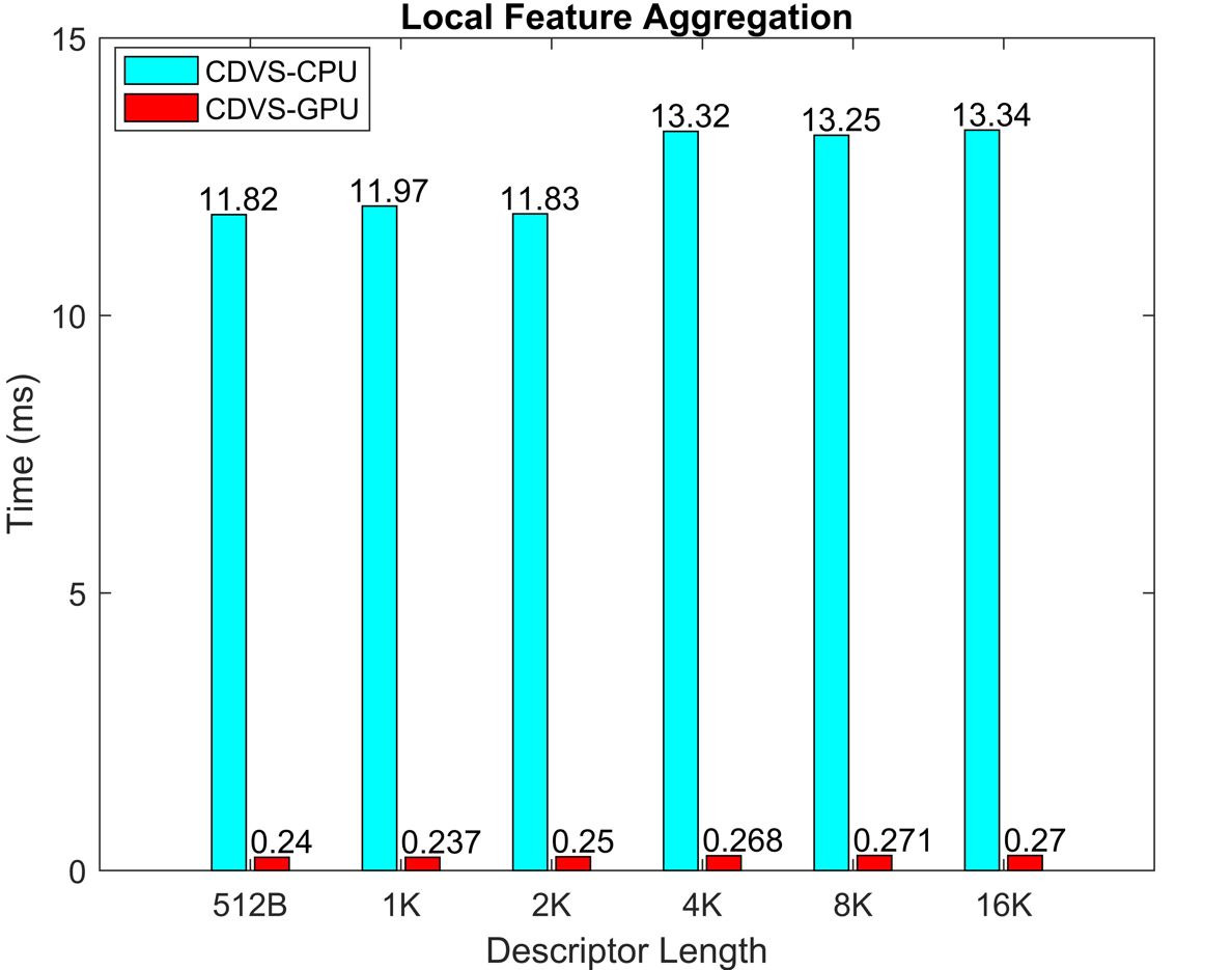
(c)

Figure 15: Complexity comparisons for different modules. (a) Interest point detection; (b) Local feature description; (c) Local feature aggregation. These results are tested on on Linux PC with Intel(R) Xeon(R) CPU E5-2650 v2@2.60GHz and a Quadro GP100 GPU.

Figure 16: The running time consumption for different modules of the proposed fast CDVS, tested on Linux PC with Intel(R) Xeon(R) CPU E5-2650 v2@2.60GHz and a Quadro GP100 GPU.

To further test the speedup of the fast CDVS encoder, we run tests on different kinds of GPUs as shown in Table III. Herein, the 11 NVIDIA GPUs are utilized in our experiment, Tesla M40, GTX1060, GTX1080 and GTX1080Ti are the popular GPUs targeting at hyper-converged systems, and the Jetson TX1 is the popular GPU for embedded systems. Specially, NVIDIA has provided us the up-to-date GPUs for the two systems, i.e., Tesla P40, P100, Titan X, Quadro GP100 and Jetson TX2, which shows the maximum speedup. Our CDVS encoder only costs $3.38\sim 5.05$ ms for VGA resolution images on popular GPUs, and $3.24\sim 3.75$ ms on the up-to-date GPUs. Even for the $1920\times 1080$ images, our encoder can extract the descriptors in real time with minimum 12.41 ms. More importantly, our CDVS encoder can extract feature descriptors for $640\times 480$ images in real time on Jetson TX2, which are the promising platform for embedded systems with low power consumption. This indicates that the CDVS can be well deployed on mobile devices to support very fast visual search. Based on comprehensive experimental results, we can claim that the CDVS using GPU-CPU hybrid computing can well support scalable image/video retrieval and analysis with real-time requirements.

TABLE III: The running time comparison of CDVS on different GPU platform, tested on Linux PC with Intel(R) Xeon(R) CPU E5-2650 v2 @ 2.60GHz, Time (ms).

GPUs	$640\times 480$	$1920\times 1080$	GPUs	$640\times 480$	$1920\times 1080$
GTX 1060	5.05	20.91	GTX 1080	3.54	12.97
Tesla M40	5.02	20.4	GTX 1080Ti	3.38	12.58
Titan X Pascal∗	3.75	15.37	Quadro GP100∗	3.27	12.41
Tesla P40	3.7	14.38	Jetson TX1	40.22	161.51
Tesla P100∗	3.56	14.61	Jetson TX2∗	28.69	138.74

TABLE IV: Performance comparison of CNNs, CDVS and their combination descriptors, tested on Linux PC with Intel(R) Xeon(R) CPU E5-2650 v2@2.60GHz and a Quadro GP100 GPU.

	mAP	Top Match	TPR@FPR=0.01	Descriptor Size	Extraction time (ms)	Memory
CDVS	0.8203	0.9093	0.918	4 KB	3.27	205 MB
RMAC	0.57	0.6638	0.456	2 KB	36.5	6635 MB
RMAC + CDVS local	0.7858	0.8921	0.913	4 KB	40.1	6715 MB
RMAC + CDVS global	0.8009	0.872	0.8714	4 KB	40.2	6840 MB
NIP-VGG-16	0.6768	0.7809	0.52	2 KB	144	6635 MB
NIP-VGG-16 + CDVS local	0.8003	0.865	0.9166	4 KB	147.6	6715 MB
NIP-VGG-16 + CDVS global	0.8508	0.9124	0.874	4 KB	147.7	6840 MB

V-D Promising Future of CDVS and CNN Feature Descriptors

CDVS provides MPEG standard compliant handcrafted visual feature descriptor with high performance, good compactness and friendly to parallel implementation. Recently, although the visual feature descriptors generated from convolutional neural network (CNN) have provide very promising performance, the performance can be further improved when combining the handcraft visual descriptors of CDVS. In [50], we have proposed a Nested Invariance Pooling (NIP) method to obtain compact and robust CNN descriptors, which are generated by applying three different pooling operations to the feature maps of CNNs in a nested way towards rotation and scale invariant feature representation. To explore the potential performance, we combine the CDVS local and global feature descriptors with two CNN features, i.e., NIP-VGG-16 [50] and RMAC [51] to perform pair matching and image retrieval.

In our experiments, the dimensions of NIP-VGG-16 and RMAC descriptors are 512. We use 4 bytes to represent each dimension, which leads to 2KB representation for NIP-VGG-16 and RMAC. Table IV shows the image retrieval and matching performance on MPEG-CDVS database. Although both CNN feature descriptors achieve good performance at low bitrate, their performances are further improved by combining CDVS descriptors. The improvements of NIP-VGG-16 with CDVS global descriptors are up to 0.0305 and 0.174 compared with CDVS and NIP-VGG-16 respectively in terms of mAP. To the best of our knowledge, the combination of CNN and CDVS achieves the best pair matching and image retrieval performance at the same descriptor length, which also has been verified in the latest proposals of the emerging MPEG Compact Descriptors for Video Analysis (CDVA)standard [52].

Although the CNN descriptors achieve promising results in computer vision applications, the extremely huge computational burdens make them heavily dependent on GPU platform. For 1000 VGA resolution images, the average running time of CNN descriptor extraction about 144 ms and 36.5 ms for NIP-VGG-16 and RMAC networks, which obviously exceed that of CDVS on the GPU platform. In additional, the CNN descriptor extraction also consumes too much memory compared with that of CDVS as shown in Table IV. Hence,it is promising to combine the CNN feature descriptors and the handcraft feature descriptors, and implement them harmonically using GPU platform, which can provide scalable descriptors for both computational resources and visual search accuracy.

VI Conclusion

We have revisited the merits of the MPEG-CDVS standard in computational cost reduction. A very fast CDVS encoder has been implemented using hybrid GPU-CPU computing. By thoroughly comparison with other state-of-the-art visual descriptors on large-scale database, the fast CDVS encoder achieves significant speedup compared with that on CPU platform (more than 35 times) while maintaining the competitive performance for image retrieval and matching. Furthermore, by incorporating the CDVS encoder with deep learning based approaches on GPU platform, we have shown that the handcraft visual feature descriptors and CNN based feature descriptors are complementary to some extent and the combination of CDVS descriptors and the CNN descriptors has achieved the state-of-the-art visual search performance over benchmarks. Especially towards real-time (mobile) visual search and augmented reality applications, how to harmoniously leverage the merits of highly efficient and low complexity handcrafted descriptors, and the state-of-the-art CNNs based descriptors via GPU or GPU-CPU hybrid computing, is a competitive and promising topic.

References

- [1] B. Girod, V. Chandrasekhar, R. Grzeszczuk, and Y. A. Reznik, “Mobile visual search: Architectures, technologies, and the emerging mpeg standard,” IEEE MultiMedia, vol. 18, no. 3, pp. 86–94, 2011.
- [2] D. G. Lowe, “Distinctive image features from scale-invariant keypoints,” International journal of computer vision, vol. 60, no. 2, pp. 91–110, 2004.
- [3] H. Bay, A. Ess, T. Tuytelaars, and L. Van Gool, “Speeded-up robust features (surf),” Computer vision and image understanding, vol. 110, no. 3, pp. 346–359, 2008.
- [4] E. Rublee, V. Rabaud, K. Konolige, and G. Bradski, “Orb: An efficient alternative to sift or surf,” in 2011 International Conference on Computer Vision, Nov 2011, pp. 2564–2571.
- [5] S. Leutenegger, M. Chli, and R. Y. Siegwart, “Brisk: Binary robust invariant scalable keypoints,” in 2011 International Conference on Computer Vision, Nov 2011, pp. 2548–2555.
- [6] L.-Y. Duan, V. Chandrasekhar, J. Chen, J. Lin, Z. Wang, T. Huang, B. Girod, and W. Gao, “Overview of the MPEG-CDVS standard,” IEEE Transactions on Image Processing, vol. 25, no. 1, pp. 179–194, 2016.
- [7] “Information technology-Multimedia content description interface-Part 13: Compact descriptors for visual search,” ISO/IEC JTC1/SC29/WG11/N14956, Oct 2014.
- [8] J. Chen, L. Y. Duan, F. Gao, J. Cai, A. C. Kot, and T. Huang, “A low complexity interest point detector,” IEEE Signal Processing Letters, vol. 22, no. 2, pp. 172–176, Feb 2015.
- [9] M. Garland, S. Le Grand, J. Nickolls, J. Anderson, J. Hardwick, S. Morton, E. Phillips, Y. Zhang, and V. Volkov, “Parallel computing experiences with cuda,” Micro, IEEE, vol. 28, no. 4, pp. 13–27, 2008.
- [10] S. Clara, “Nvidia cuda compute unified device architecture: Programming guide version 1.1.”
- [11] S. Heymann, K. Müller, A. Smolic, B. Froehlich, and T. Wiegand, “SIFT implementation and optimization for general-purpose GPU,” International Conference in Central Europe on Computer Graphics, Visualization and Computer Vision, 2007.
- [12] C. Wu, “SiftGPU: A GPU implementation of scale invariant feature transform (SIFT),” 2007.
- [13] B. Rister, G. Wang, M. Wu, and J. R. Cavallaro, “A fast and efficient SIFT detector using the mobile GPU,” in 2013 IEEE International Conference on Acoustics, Speech and Signal Processing, 2013, pp. 2674–2678.
- [14] C. Lee, C. E. Rhee, and H.-J. Lee, “Complexity Reduction by Modified Scale-Space Construction in SIFT Generation Optimized for a Mobile GPU,” IEEE Transactions on Circuits and Systems for Video Technology, 2016.
- [15] CUDASIFT, “https://github.com/Celebrandil/CudaSift,” 2007.
- [16] G. Wang, B. Rister, and J. R. Cavallaro, “Workload analysis and efficient OpenCL-based implementation of SIFT algorithm on a smartphone,” in Global Conference on Signal and Information Processing (GlobalSIP), 2013 IEEE, 2013, pp. 759–762.
- [17] D. Patlolla, S. Voisin, H. Sridharan, and A. Cheriyadat, “GPU accelerated textons and dense sift features for human settlement detection from high-resolution satellite imagery,” GeoComp, 2015.
- [18] N. Cornelis and L. Van Gool, “Fast scale invariant feature detection and matching on programmable graphics hardware,” in Computer Vision and Pattern Recognition Workshops, 2008. CVPRW’08. IEEE Computer Society Conference on, 2008, pp. 1–8.
- [19] W. Ma, L. Cao, L. Yu, G. Long, and Y. Li, “GPU-FV: Realtime Fisher Vector and Its Applications in Video Monitoring,” arXiv preprint arXiv:1604.03498, 2016.
- [20] A. Krizhevsky, I. Sutskever, and G. E. Hinton, “Imagenet classification with deep convolutional neural networks,” in Advances in neural information processing systems, 2012, pp. 1097–1105.
- [21] L. Zheng, Y. Yang, and Q. Tian, “SIFT meets CNN: a decade survey of instance retrieval,” arXiv preprint arXiv:1608.01807, 2016.
- [22] Y. Jia, E. Shelhamer, J. Donahue, S. Karayev, J. Long, R. Girshick, S. Guadarrama, and T. Darrell, “Caffe: Convolutional architecture for fast feature embedding,” in Proceedings of the 22nd ACM international conference on Multimedia. ACM, 2014, pp. 675–678.
- [23] M. Abadi, A. Agarwal, P. Barham, E. Brevdo, Z. Chen, C. Citro, G. S. Corrado, A. Davis, J. Dean, M. Devin et al., “Tensorflow: Large-scale machine learning on heterogeneous distributed systems,” arXiv preprint arXiv:1603.04467, 2016.
- [24] D. Pau, E. Napoli, G. Lopez, E. Plebani, A. BRUNA, and D. SORENSEN, “Fourier transform Based interest point detector using LoG frequency response,” ISO/IEC JTC1/SC29/WG11/M28076, Jan 2013.
- [25] Z. Liu, Q. Zhou, and X. Guojun, “Huawei s Response to CE 4: Preliminary Results by Fourier Transform Based LOG,” ISO/IEC JTC1/SC29/WG11/M28090, Jan 2013.
- [26] C. Jie, L.-Y. Duan, T. Huang, W. Gao, A. C. Kot, M. Balestri, G. Francini, and S. Lepsøy, “CDVS CE1: A low complexity detector ALP_BFLoG,” ISO/IEC JTC1/SC29/WG11/M33159, Oct 2014.
- [27] C. Jie, L.-Y. Duan, T. Huang, and W. Gao, “Peking University Response to CE1: Improved BFLoG Interest Point Detector,” ISO/IEC JTC1/SC29/WG11/M31399, Oct 2013.
- [28] G. Francini, S. Lepsoy, and M. Balestri, “CDVS: Telecom Italia s response to CE1 interest point detection,” ISO/IEC JTC1/SC29/WG11/M30256, Jul 2013.
- [29] P. Carr and D. Madan, “Option valuation using the fast fourier transform,” Journal of computational finance, vol. 2, no. 4, pp. 61–73, 1999.
- [30] L.-T. Cheok, J. Song, and K. Park, “CDVS: Telecom Italia s response to CE1 interest point detection,” ISO/IEC JTC1/SC29/WG11/M23822, Feb 2012.
- [31] W. Chunyu, L.-Y. Duan, C. Jie, T. Huang, and W. Gao, “Reference results of key point reduction,” ISO/IEC JTC1/SC29/WG11/M23929, Feb 2012.
- [32] G. Francini, S. Lepsøy, and M. Balestri, “Selection of local features for visual search,” Signal Processing: Image Communication, vol. 28, no. 4, pp. 311–322, 2013.
- [33] G. Francini, S. Lepsoy, and M. Balestri, “Description of Test Model under Consideration for CDVS,” ISO/IEC JTC1/SC29/WG11/N12367, Feb 2012.
- [34] ——, “Telecom Italia Response to the CDVS Core Experiment 2,” ISO/IEC JTC1/SC29/WG11/M24737, Apr 2012.
- [35] H. Jegou, M. Douze, and C. Schmid, “Product quantization for nearest neighbor search,” Pattern Analysis and Machine Intelligence, IEEE Transactions on, vol. 33, no. 1, pp. 117–128, 2011.
- [36] J. Chen, L.-Y. Duan, C. Wang, T. Huang, and W. Gao, “Peking Univ. Response to CE 2: Improvements of the SCFV Global Descriptor,” ISO/IEC JTC1/SC29/WG11/M22806, Oct 2011.
- [37] C. Jie, L.-Y. Duan, T. Huang, and W. Gao, “CDVS:CE2: Multi-Stage Vector Quantization for Low Memory Descriptors,” ISO/IEC JTC1/SC29/WG11/M24780, Apr 2012.
- [38] D. Chen, S. Tsai, V. Chandrasekhar, G. Takacs, H. Chen, R. Vedantham, R. Grzeszczuk, and B. Girod, “Residual enhanced visual vectors for on-device image matching,” in Signals, Systems and Computers (ASILOMAR), 2011 Conference Record of the Forty Fifth Asilomar Conference on. IEEE, 2011, pp. 850–854.
- [39] D. Chen, V. Chandrasekhar, G. Takacs, S. Tsai, M. Makar, R. Vedantham, R. Grzeszczuk, and B. Girod, “Improvements to the Test Model Under Consideration with a Global Descriptor,” ISO/IEC JTC1/SC29/WG11/M23578, Feb 2012.
- [40] S. S. Husain and M. Bober, “Improving large-scale image retrieval through robust aggregation of local descriptors,” IEEE Transactions on Pattern Analysis and Machine Intelligence, 2016.
- [41] M. Bober, S. Husain, S. Paschalakis, and K. Wnukowicz, “Improving performance and usability of CDVS TM7 with a Robust Visual Descriptor (RVD) - CE 2 Proposal from University of Surrey and Visual Atoms,” ISO/IEC JTC1/SC29/WG11/M31426, Oct 2013.
- [42] J. Lin, L.-Y. Duan, Y. Huang, S. Luo, T. Huang, and W. Gao, “Rate-adaptive compact fisher codes for mobile visual search,” IEEE Signal Processing Letters, vol. 21, no. 2, pp. 195–198, 2014.
- [43] J. Lin, L.-Y. Duan, Z. Wang, T. Huang, and W. Gao, “Peking Univ. Response to CE 2: Improvements of the SCFV Global Descriptor,” ISO/IEC JTC1/SC29/WG11/M31401, Oct 2013.
- [44] “Evaluation framework for compact descriptors for visual search,” ISO/IEC JTC1/SC29/WG11/N12202, Jul 2011.
- [45] H. Jegou, M. Douze, and C. Schmid, “Hamming embedding and weak geometric consistency for large scale image search,” Computer Vision–ECCV 2008, pp. 304–317, 2008.
- [46] CDVS Patches, 2013. [Online]. Available: http://blackhole1.stanford.edu/vijayc/cdvs patches.tar
- [47] S. Winder, G. Hua, and M. Brown, “Picking the best daisy,” in Computer Vision and Pattern Recognition, 2009. CVPR 2009. IEEE Conference on. IEEE, 2009, pp. 178–185.
- [48] P. Alcantarilla, J. Nuevo, and A. Bartoli, “Fast explicit diffusion for accelerated features in nonlinear scale spaces,” in British Machine Vision Conference, 2013, pp. 13.1–13.11.
- [49] G. Levi and T. Hassner, “Latch: Learned arrangements of three patch codes,” in 2016 IEEE Winter Conference on Applications of Computer Vision (WACV), March 2016, pp. 1–9.
- [50] Y. Lou, Y. Bai, J. Lin, S. Wang, J. Chen, V. Chandrasekhar, L.-Y. Duan, T. Huang, A. C. Kot, and W. Gao, “Compact deep invariant descriptors for video retrieval,” in 2017 Data Compression Conference, 2017.
- [51] G. Tolias, R. Sicre, and H. Jégou, “Particular object retrieval with integral max-pooling of cnn activations,” arXiv preprint arXiv:1511.05879, 2015.
- [52] Y. Lou, F. Gao, Y. Bai, J. Lin, S. Wang, J. Chen, C. Gan, V. Chandrasekhar, L. Duan, T. Huang, and A. Kot, “Improved retrieval and matching with CNN feature for CDVA,” ISO/IEC JTC1/SC29/WG11/M39219, Oct 2016.