Random Iteration of Cylinder Maps and diffusive behavior away from resonances

Abstract

In this paper we propose a model of random compositions of cylinder maps, which in the simplified form is as follows: let $(\theta,r)\in\mathbb{T}\times\mathbb{R}=\mathbb{A}$ and

$$f_{\pm 1}:\left(\begin{array}[]{c}\theta\\ r\end{array}\right) \longmapsto \left(\begin{array}[]{c}\theta+r+\varepsilon u_{\pm 1}(\theta,r)\\ r+\varepsilon v_{\pm 1}(\theta,r)\end{array}\right),$$ (5)

where $u_{\pm}$ and $v_{\pm}$ are smooth and $v_{\pm}$ are trigonometric polynomials in $\theta$ such that $\int v_{\pm}(\theta,r)\,d\theta=0$ for each $r$. We study the random compositions

$$(\theta_{n},r_{n})=f_{\omega_{n-1}}\circ\dots\circ f_{\omega_{0}}(\theta_{0},r_{0}),$$

where $\omega_{k}=\pm 1$ with equal probability. We show that under non-degeneracy hypotheses and away from resonances for $n\sim\varepsilon^{-2}$ the distributions of $r_{n}-r_{0}$ weakly converge to a stochastic diffusion process with explicitly computable drift and variance.

In the case $u_{\pm}(\theta)=v_{\pm}(\theta)$ are trigonometric polynomials of zero average we prove a vertical central limit theorem, namely, for $n\sim\varepsilon^{-2}$ the distributions of $r_{n}-r_{0}$ weakly converge to the normal distribution $\mathcal{N}(0,\sigma^{2})$ with $\sigma^{2}=\frac{1}{4}\int(v_{+}(\theta)-v_{-}(\theta))^{2}\,d\theta$.

The random model (5) up to higher order terms in $\varepsilon$ is conjugate to a restrictions to a Normally Hyperbolic Invariant Lamination of the generalized Arnold example (see [23, 28]). Combining the result of this paper with [8, 23, 28] we show formation of stochastic diffusive behaviour for the generalized Arnold example.

1 Introduction

1.1 Motivation: Arnold diffusion and instabilities

By Arnold-Liouville theorem a completely integrable Hamiltonian system can be written in action-angle coordinates, namely, for action $p$ in an open set $U\subset\mathbb{R}^{n}$ and angle $\theta$ on an $n$-dimensional torus $\mathbb{T}^{n}$ there is a function $H_{0}(p)$ such that equations of motion have the form

$$\dot{\theta}=\omega(p),\quad\dot{p}=0,\qquad\text{ where }\ \omega(p):=\partial_{p}H_{0}(p).$$

The phase space is foliated by invariant $n$-dimensional tori $\{p=p_{0}\}$ with either periodic or quasi-periodic motions $\theta(t)=\theta_{0}+t\,\omega(p_{0})$ (mod 1). There are many different examples of integrable systems (see e.g. wikipedia).

It is natural to consider small Hamiltonian perturbations

$$H_{\varepsilon}(\theta,p)=H_{0}(p)+\varepsilon H_{1}(\theta,p),\qquad\theta\in\mathbb{T}^{n},\ p\in U$$

where $\varepsilon$ is small. The new equations of motion become

$$\dot{\theta}=\omega(p)+\varepsilon\partial_{p}H_{1},\quad\dot{p}=-\varepsilon\partial_{\theta}H_{1}.\qquad\qquad$$

In the sixties, Arnold [1] (see also [2, 3]) conjectured that for a generic analytic perturbation there are orbits $(\theta,p)(t)$ for which the variation of the actions is of order one, i.e. $\|p(t)-p(0)\|$ that is bounded from below independently of $\varepsilon$ for all $\varepsilon$ sufficiently small.

See [5, 9, 26, 27, 32, 33] about recent progress proving this conjecture for convex Hamiltonians.

1.2 KAM stability

Obstructions to any form of instability, in general, and to Arnold diffusion, in particular, are widely known, following the works of Kolmogorov, Arnold, and Moser, nowadays called KAM theory. The fundamental result says that for a properly non-degenerate $H_{0}$ and for all sufficiently regular perturbations $\varepsilon H_{1}$, the system defined by $H_{\varepsilon}$ still has many invariant $n$-dimensional tori. These tori are small deformation of unperturbed tori and measure of the union of these invariant tori tends to the full measure as $\varepsilon$ goes to zero.

One consequence of KAM theory is that for $n=2$ there are no instabilities. Indeed, generic energy surfaces $S_{E}=\{H_{\varepsilon}=E\}$ are $3$-dimensional manifolds whereas KAM tori are $2$-dimensional. Thus, KAM tori separate surfaces $S_{E}$ and prevent orbits from diffusing.

1.3 A priori unstable systems

In [1] Arnold proposed to study the following important example

$$H_{\varepsilon}(p,q,I,\varphi,t)=\dfrac{I^{2}}{2}+H_{0}(p,q)+\varepsilon H_{1}(p,q,I,\varphi,t):=$$

$$=\underbrace{\dfrac{\ \ \ \ \ \ \ I^{2}\ \ \ \ \ \ \ }{2}}_{harmonic\ oscillator}+\underbrace{\dfrac{p^{2}}{2}+(\cos q-1)}_{pendulum}+\varepsilon H_{1}(p,q,I,\varphi,t),$$

where $q,\varphi,t\in\mathbb{T}$ — angles, $p,I\in\mathbb{R}$ — actions (see Figure 1), $H_{1}=(\cos q-1)(\cos\varphi+\cos t)$.

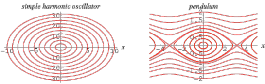
Figure 1: The rotor times the pendulum

For $\varepsilon=0$ the system is a direct product of the harmonic oscillator $\ddot{\varphi}=0$ and the pendulum $\ddot{q}=\sin q$. Instabilities occur when the $(p,q)$-component follows the separatrices $H_{0}(p,q)=0$ and passes near the saddle $(p,q)=(0,0)$. Equations of motion for $H_{\varepsilon}$ have a (normally hyperbolic) invariant cylinder $\Lambda_{\varepsilon}$ which is $\mathcal{C}^{1}$ close to $\Lambda_{0}=\{p=q=0\}$. Systems having an invariant cylinder with a family of separatrix loops are called a priori unstable. Since they were introduced by Arnold [1], they received a lot of attention both in mathematics and physics community see e.g. [4, 10, 9, 12, 14, 22, 45, 46].

Chirikov [11] and his followers made extensive numerical studies for the Arnold example. He conjectured that the $I$-displacement behaves randomly, where randomness is due to choice of initial conditions near $H_{0}(p,q)=0$.

More exactly, integration of solutions whose “initial conditions” randomly chosen $\varepsilon$-close to $H_{0}(p,q)=0$ and integrated over time $\sim\varepsilon^{-2}\ln\varepsilon^{-1}$ -time. This leads to the $I$–displacement being of order of one and having some distribution. This coined the name for this phenomenon: Arnold diffusion.

Let $\varepsilon=0.01$ and $T=\varepsilon^{-2}\ln\varepsilon^{-1}$. On Fig. 1.3 we present several histograms plotting displacement of the $I$-component after time $T,2T,4T,8T$ with 6 different groups of initial conditions, and histograms of $10^{6}$ points. In each group we start with a large set of initial conditions close to $p=q=0,\ I=I^{*}$. One of the distinct features is that only one distribution (a) is close to symmetric, while in all others have a drift.

A similar stochastic behaviour was observed numerically in many other nearly integrable problems ([11] pg. 370, [17, 30], see also [42]). To give another illustrative example consider motion of asteroids in the asteroid belt.

1.4 Fluctuations of eccentricity in Kirkwood gaps in the asteroid belt

The asteroid belt is located between orbits of Mars and Jupiter and has around one million asteroids of diameter of at least one kilometer. When astronomers build a histogram based on orbital period of asteroids there are well known gaps in distribution called Kirkwood gaps (see Figure below).

These gaps occur when the ratio of periods of an asteroid and Jupiter is a rational with small denominator: $1/3,2/5,3/7,1/2$. This corresponds to so called mean motion resonances for the three body problem.

Wisdom [47] made a numerical analysis of dynamics at the $1/3$ resonance and observed drastic jumps of eccentricity of asteroids, which are large enough so that an orbit of asteroid starts crossing the orbit of Mars. Once orbits do cross, they eventually undergo ejection, or collision, or capture. Later it was shown that this mechanism of jumps applies to the $2/5$ resonance. However, resonances $3/7$ and $1/2$ exhibited a different nature of instability (see e.g. [37]).

In [18] for small (unrealistic) eccentricity of Jupiter, we construct a dynamical structure along the $1/3$ resonance which hypothetically leads to random fluctuations of eccentricity. Using this structure we prove existence of orbits whose eccentricity change by $\mathcal{O}(1)$ for the restricted planar three body problem.

Outside of these resonances one could argue that KAM theory provides stability see e.g. [38].

1.5 Random iteration of cylinder maps

Consider the time one map of $H_{\varepsilon}$, denoted

$$F_{\varepsilon}:(p,q,I,\varphi)\to(p^{\prime},q^{\prime},I^{\prime},\varphi^{\prime}).$$

It turns out that for initial conditions in certain domains $\varepsilon$-close to $H_{0}(p,q)=0$, one can define a return map to an $\mathcal{O}(\varepsilon)$-neighborhood of $(p,q)=0$. Often such a map is called a separatrix map and in the $2$-dimensional case was introduced by the physicists Filonenko-Zaslavskii [19]. In multidimensional setting such a map was defined and studied by Treschev [39, 44, 45, 46].

It turns out that starting near $(p,q)=0$ and iterating $F_{\varepsilon}$ until the orbit comes back $(p,q)=0$ leads to a family of maps of a cylinder

$$f_{\varepsilon,p,q}:(I,\varphi)\to(I^{\prime},\varphi^{\prime}),\qquad(I,\varphi)\in\mathbb{A}=\mathbb{R}\times\mathbb{T}$$

which are close to integrable. Since at $(p,q)=0$ the $(p,q)$-component has a saddle, there is a sensitive dependence on initial condition in $(p,q)$ and returns do have some randomness in $(p,q)$. The precise nature of this randomness at the moment is not clear. There are several coexisting behaviours, including unstable diffusive, stable quasi-periodic, orbits can stick to KAM tori. Which behavior is dominant is yet to be understood. May be also the mechanism of capture into resonances [16] is also relevant in this setting.

In [28] we construct a normally hyperbolic invariant lamination (NHIL) for an open class of trigonometric perturbations $H_{1}=P(\exp(i\varphi),\,\exp(it),\,\exp(iq)).$

Constructing unstable orbits along a NHIL is also discussed in [15]. In general, NHILs give rise to a skew shift. For example, let $\Sigma=\{-1,1\}^{\mathbb{Z}}$ be the space of infinite sequences of $-1$’s and $1$’s and $\sigma:\Sigma\to\Sigma$ be the standard shift.

Consider a skew product of cylinder maps

$$F:\mathbb{A}\times\Sigma\to\mathbb{A}\times\Sigma,\qquad F(r,\theta;\omega)=(f_{\omega}(r,\theta),\sigma\omega),$$

where each $f_{\omega}(r,\theta)$ is a nearly integrable cylinder maps, in the sense that it almost preserves the $r$-component .

The goal of the present paper is to study a wide enough class of skew products so that they arise in Arnold’s example with a trigonometric perturbation of the above type (see [23, 28]).

Now we formalize our model and present the main result.

1.6 Diffusion processes and infinitesimal generators

We recall some basic probabilistic notions. Consider a Brownian motion $\{B_{t},\,t\geq 0\}$.

It is a properly chosen limit of the standard random walk. A generalisation of a Brownian motion is a diffusion process or an Ito diffusion. To define it let $(\Omega,\Sigma,P)$ be a probability space. Let $R:[0,+\infty)\times\Omega\to\mathbb{R}$. It is called an Ito diffusion if it satisfies a stochastic differential equation of the form

$$\mathrm{d}R_{t}=b(R_{t})\,\mathrm{d}t+\sigma(R_{t})\,\mathrm{d}B_{t},$$ (6)

where $B_{t}$ is a Brownian motion and $b:\mathbb{R}\to\mathbb{R}$ and $\sigma:\mathbb{R}\to\mathbb{R}$ are Lipschitz functions called the drift and the variance respectively. For a point $r\in\mathbb{R}$, let $\mathbb{P}_{r}$ denote the law of $X$ given initial data $R_{0}=r$, and let $\mathbb{E}_{r}$ denote expectation with respect to $\mathbb{P}_{r}$.

The infinitesimal generator of $R$ is the operator $A$, which is defined to act on suitable functions $f:\mathbb{R}\to\mathbb{R}$ by

$$Af(r)=\lim_{t\downarrow 0}\dfrac{\mathbb{E}_{r}[f(R_{t})]-f(r)}{t}.$$

The set of all functions $f$ for which this limit exists at a point $r$ is denoted $D_{A}(r)$, while $D_{A}$ denotes the set of all $f$’s for which the limit exists for all $r\in\mathbb{R}$. One can show that any compactly-supported $\mathcal{C}^{2}$ function $f$ lies in $D_{A}$ and that

$$Af(r)=b(r)\dfrac{\partial f}{\partial r}+\dfrac{1}{2}\sigma^{2}(r)\dfrac{\partial^{2}f}{\partial r\partial r}.$$ (7)

The distribution of a diffusion process is characterized by the drift $b(r)$ and the variance $\sigma(r)$.

2 The model and statement of the main result

Let $\varepsilon>0$ be a small parameter and $l\geq 7$, $s\geq 0$ be integers. Denote by $\mathcal{O}_{s}(\varepsilon)$ a $\mathcal{C}^{s}$ function whose $\mathcal{C}^{s}$ norm is bounded by $C\varepsilon$ with $C$ independent of $\varepsilon$. Similar definition applies for a power of $\varepsilon$. As before $\Sigma$ denotes $\{-1,1\}^{\mathbb{Z}}$ and $\omega=(\dots,\omega_{0},\dots)\in\Sigma$.

Consider nearly integrable maps

$$f_{\omega}:\mathbb{T}\times\mathbb{R} \longrightarrow \mathbb{T}\times\mathbb{R}\qquad\qquad\qquad\qquad\qquad\qquad$$

$$f_{\omega}:\left(\begin{array}[]{c}\theta\\ r\end{array}\right) \longmapsto \left(\begin{array}[]{c}\theta+r+\varepsilon u_{\omega_{0}}(\theta,r)+\mathcal{O}_{s}(\varepsilon^{1+a},\omega)\\ r+\varepsilon v_{\omega_{0}}(\theta,r)+\varepsilon^{2}w_{\omega_{0}}(\theta,r)+\mathcal{O}_{s}(\varepsilon^{2+a},\omega)\end{array}\right),$$ (12)

for $\omega_{0}\in\{-1,1\}$, where $u_{\omega_{0}},\ v_{\omega_{0}},$ and $w_{\omega_{0}}$ are bounded $\mathcal{C}^{l}$ functions, $1$-periodic in $\theta$, $\mathcal{O}_{s}(\varepsilon^{1+a},\omega)$ and $\mathcal{O}_{s}(\varepsilon^{2+a},\omega)$ denote remainders depending on $\omega$ and uniformly $\mathcal{C}^{s}$ bounded in $\omega$, and $a>1/2$. Assume

$$\max|v_{i}(\theta,r)|\leq 1,$$

where maximum is over $i=\pm 1$ and all $(\theta,r)\in\mathbb{A}$, otherwise, renormalize $\varepsilon$, and

$$\|u_{i}\|_{\mathcal{C}^{6}},\|v_{i}\|_{\mathcal{C}^{6}},\|w_{i}\|_{\mathcal{C}^{6}}\leq C$$

for some $C>0$ independent of $\varepsilon$.

Even if the maps $f_{\omega}$ depend on the full sequence $\omega$, the dependence on the elements of $\omega_{k}$, $k\neq 0$, is rather weak since only appear in the small remainder. Therefore, we abuse notation and we denote these maps as $f_{1}$ and $f_{-1}$. Certainly we do not have two but an infinite number of maps. Nevertheless, they can be treated as just two maps since the remainders are negligible.

We study the random iterations of these maps $f_{1}$ and $f_{-1}$, assuming that at each step the probability of performing either map is $1/2$. The importance of understanding iterations of several maps for problems of diffusion is well known (see e.g. [25, 38]).

Denote the expected potential and the difference of potentials by

$$\begin{split}\mathbb{E}u(\theta,r)&:=\frac{1}{2}(u_{1}(\theta,r)+u_{-1}(\theta,r)),\ \ \ \mathbb{E}v(\theta,r):=\frac{1}{2}(v_{1}(\theta,r)+v_{-1}(\theta,r)),\\ u(\theta,r)&:=\frac{1}{2}(u_{1}(\theta,r)-u_{-1}(\theta,r)),\ \ \ v(\theta,r):=\frac{1}{2}(v_{1}(\theta,r)-v_{-1}(\theta,r)).\end{split}$$

Suppose the following assumptions hold:

• (zero average) For each $r\in\mathbb{R}$ and $i=\pm 1$ we have $\int v_{i}(\theta,r)\,d\theta=0$.

• for each $r\in\mathbb{R}$ we have $\int_{0}^{1}\ v^{2}(\theta,r)d\theta=:\sigma(r)\neq 0$;

• The functions $v_{i}(\theta,r)$ are trigonometric polynomials in $\theta$, i.e. for some positive integer $d$ we have

  $$v_{i}(\theta,r)=\sum_{k\in\mathbb{Z},\ 0<|k|\leq d}v_{{i}}^{(k)}(r)e^{2\pi ik\theta}.$$

• (no common zeroes) For each integer $n\in\mathbb{Z}$ potentials $v_{1}(\theta,n)$ and $v_{-1}(\theta,n)$ have no common zeroes and, equivalently, $f_{1}$ and $f_{-1}$ have no fixed points.

• (no common periodic orbits) Take any rational $r=p/q\in\mathbb{Q}$ with $p,q$ relatively prime, $1\leq|q|\leq 2d$ and any $\theta^{*}\in\mathbb{T}$ such that for all $\theta$ either

  $$\sum_{k=1}^{q}v_{-1}\left(\theta+\frac{k}{q},\frac{p}{q}\right)\neq 0$$

  or

  $$\sum_{k=1}^{q}\left[v_{-1}\left(\theta+\frac{k}{q},\frac{p}{q}\right)-v_{1}\left(\theta+\frac{k}{q},\frac{p}{q}\right)\right]^{2}\neq 0.$$

  This prohibits $f_{1}$ and $f_{-1}$ to have common periodic orbits of period $|q|$.

• (no degenerate periodic points) Suppose for any rational $r=p/q\in\mathbb{Q}$ with $p,q$ relatively prime, $1\leq|q|\leq 2d$, the function:

  $$\mathbb{E}v_{p,q}(\theta,r)=\sum_{\begin{subarray}{c}k\in\mathbb{Z}\\ 0<|kq|<d\end{subarray}}\mathbb{E}v^{kq}(r)e^{2\pi ikq\theta}$$

  has distinct non-degenerate zeroes, where $\mathbb{E}v^{j}(r)$ denotes the $j$–th Fourier coefficient of $\mathbb{E}v(\theta,r)$.

For $\omega\in\{-1,1\}^{\mathbb{Z}}$ we can rewrite the maps $f_{\omega}$ in the following form:

$$f_{\omega}\left(\begin{array}[]{c}\theta\\ r\end{array}\right)\longmapsto\left(\begin{array}[]{c}\theta+r+\varepsilon\mathbb{E}u(\theta,r)+\varepsilon\omega_{0}u(\theta,r)+\mathcal{O}_{s}(\varepsilon^{1+a},\omega)\\ r+\varepsilon\mathbb{E}v(\theta,r)+\varepsilon\omega_{0}v(\theta,r)+\varepsilon^{2}w_{\omega_{0}}(\theta,r)+\mathcal{O}_{s}(\varepsilon^{2+a},\omega)\end{array}\right).$$

Let $n$ be a positive integer and $\omega_{k}\in\{-1,1\}$, $k=0,\dots,n-1$, be independent random variables with $\mathbb{P}\{\omega_{k}=\pm 1\}=1/2$ and $\Omega_{n}=\{\omega_{0},\dots,\omega_{n-1}\}$. Given an initial condition $(\theta_{0},r_{0})$ we denote

$$(\theta_{n},r_{n}):=f^{n}_{\Omega_{n}}(\theta_{0},r_{0})=f_{\omega_{n-1}}\circ f_{\omega_{n-2}}\circ\cdots\circ f_{\omega_{0}}(\theta_{0},r_{0}).$$

A straightforward calculation shows that:

$$\begin{array}[]{rcl}\theta_{n}&=&\displaystyle\theta_{0}+nr_{0}+\varepsilon\left(\sum_{k=0}^{n-1}\mathbb{E}u(\theta_{k},r_{k})+\sum_{k=0}^{n-2}(n-k-1)\mathbb{E}v(\theta_{k},r_{k})\right)\\ &&\displaystyle+\varepsilon\left(\sum_{k=0}^{n-1}\omega_{k}u(\theta_{k},r_{k})+\sum_{k=0}^{n-2}(n-k-1)\omega_{k}v(\theta_{k},r_{k})\right)+\mathcal{O}_{s}(n\varepsilon^{1+a})\vskip 12.0pt plus 4.0pt minus 4.0pt\\ r_{n}&=&\displaystyle r_{0}+\varepsilon\sum_{k=0}^{n-1}\mathbb{E}v(\theta_{k},r_{k})+\varepsilon\sum_{k=0}^{n-1}\omega_{k}v(\theta_{k},r_{k})+\mathcal{O}_{s}(n\varepsilon^{2+a})\end{array}$$ (13)

Theorem 2.1.

Assume that, in the notations above, conditions [H0-H5] hold and take $r_{0}\in\mathbb{R}$. Let $n_{\varepsilon}\varepsilon^{2}\to s>0$ as $\varepsilon\to 0$ for some $s>0$. Then as $\varepsilon\to 0$ the distribution of $r_{n_{\varepsilon}}-r_{0}$ converges weakly to $R_{s}$, where $R_{\bullet}$ is a diffusion process of the form (6), with the drift and the variance

$$b(R)=\int_{0}^{1}E_{2}(\theta,R)\,d\theta,\qquad\sigma^{2}(R)=\int_{0}^{1}v^{2}(\theta,R)\,d\theta.$$ (14)

for certain function $E_{2}$, defined in (23).

Remarks

• If the map is area preserving and exact, one can check that

  $$b(R)=0$$

  (see Corollary 4.3).

• In the case that $u_{\pm 1}=v_{\pm 1}$ and that they are independent of $r$, we have two area-preserving standard maps. In this case the assumptions become

  • [H0] $\int v_{i}(\theta)d\theta=0$ for $i=\pm 1$;

  • [H1] $v$ is not identically zero;

  • [H2] the functions $v_{i}$ are trigonometric polynomials.

  A good example is $u_{1}(\theta)=v_{1}(\theta)=\cos 2\pi\theta$ and $u_{-1}(\theta)=v_{-1}(\theta)=\sin 2\pi\theta$. In this case

  $$b(r):=\int_{0}^{1}E_{2}(\theta,r)d\theta\equiv 0,\qquad\sigma^{2}=\int_{0}^{1}v^{2}(\theta)\,d\theta=\frac{1}{4}$$

  and for $n\leq\varepsilon^{-2}$ the distribution $r_{n}-r_{0}$ converges to the zero mean variance $\varepsilon n^{2}\sigma^{2}$ normal distribution, denoted $\mathcal{N}(0,\varepsilon n^{2}\sigma^{2})$. More generally, we have the following “vertical central limit theorem”:

  Theorem 2.2.

  Assume that in the notations above conditions [H0-H5] hold. Let $n_{\varepsilon}\varepsilon^{2}\to s>0$ as $\varepsilon\to 0$ for some $s>0$. Then as $\varepsilon\to 0$ the distribution of $r_{n_{\varepsilon}}-r_{0}$ converges weakly to a normal random variable $\mathcal{N}(0,s^{2}\sigma^{2}).$

• Numerical experiments of Moeckel [36] show that no common fixed points and periodic orbits (see Hypotheses [H3] and [H4]) is not neccessary to deal with the resonant zones. One could probably replace it by a weaker non-degeneracy condition, e.g. that the linearization of maps $f_{\pm 1}$ at the common fixed and periodic points are different.

• In [40] Sauzin studies random iterations of the standard maps

  $$(\theta,r)\to(\theta+r+\lambda\phi(\theta),r+\lambda\phi(\theta)),$$

  where $\lambda$ is chosen randomly from $\{-1,0,1\}$ and proves the vertical central limit theorem; In [34, 41] Marco-Sauzin present examples of nearly integrable systems having a set of initial conditions exhibiting the vertical central limit theorem.

• In [31] Marco derives a sufficient condition for a skew-shift to be a step skew-shift.

• The condition [H2] that the functions $v_{i}$ are trigonometric polynomials in $\theta$ seems redundant too, however, removing it leads to considerable technical difficulties (see Section 3.2). In short, for perturbations by a trigonometric polynomial there are finitely many resonant zones. This finiteness considerably simplifies the analysis.

• One can replace $\Sigma=\{-1,1\}^{\mathbb{Z}}$ with $\Sigma_{N}=\{0,1,\dots,N-1\}^{\mathbb{Z}}$, consider any finite number of maps of the form (2) and a transitive Markov chain with some transition probabilities. If conditions [H0–H5] are satisfied for the proper averages $\mathbb{E}v$ of $v$, then Theorem 2.1 holds.

3 Strategy of the proof

The random map (13) has two significantly different regimes: resonant and non-resonant. In this paper we analyze (13) away from resonances. The resonance setting is analyzed in [8]. The main result of [8] is presented in Section 3.5.

We proceed to define the two regimes. Let

$$\mathcal{N}=\{k\in\mathbb{Z}:(\mathbb{E}u^{k},\mathbb{E}v^{k})\neq 0\}.$$ (15)

Fix $\beta>0$. Then, the $\beta$-non-resonant domain is defined as

$$\mathcal{D}_{\beta}=\left\{r\in\mathbb{R}:\forall q\in\mathcal{N},\ p\in\mathbb{Z}\ \text{we have }\ \left|r-\frac{p}{q}\right|\geq 2\beta\right\}.$$ (16)

Notice that, by Hypothesis H2, $\mathcal{D}_{\beta}$ contains the subset of $\mathbb{R}$ which excludes the $2\beta$-neighborhoods of all rational numbers $p/q$ with $0<|q|\leq 2d$. Analogously, we can define the resonant domains associated to a rational $p/q$ with $q\in\mathcal{N}$ as

$$\mathcal{R}^{p/q}_{\beta}=\left\{r\in\mathbb{R}:\ \left|r-\frac{p}{q}\right|\leq 2\beta\right\}.$$ (17)

3.1 Strip decomposition

Fix $\gamma\in(0,1)$. We divide the non-resonant zone of the cylinder, namely $\mathbb{T}\times\mathcal{D}_{\beta}$ (see (16)), in strips $\mathbb{T}\times I^{j}_{\gamma}$, where $I^{j}_{\gamma}\subset\mathcal{D}_{\beta},\ j\in\mathbb{Z}$, are intervals of length $\varepsilon^{\gamma}$. Then we study how the random variable $r_{n}-r_{0}$ behaves in each strip. More precisely, decompose the process $r_{n}(\omega),n\in\mathbb{Z}_{+}$ into infinitely many time intervals defined by stopping times

$$0<n_{1}<n_{2}<\dots,$$ (18)

where

• $r_{n_{i}}(\omega)$ is $\varepsilon$-close to the boundary between $I^{j}_{\gamma}$ and $I^{j+1}_{\gamma}$ for some $j\in\mathbb{Z}$

• $r_{n_{i+1}}(\omega)$ is $\varepsilon$-close to the other boundary of either $I^{j}_{\gamma}$ or of $I^{j+1}_{\gamma}$ and $n_{i+1}>n_{i}$ is the smallest integer with this property.

Since $\varepsilon\ll\varepsilon^{\gamma}$, being $\varepsilon$-close to the boundary of $I^{j}_{\gamma}$ with a negligible error means jump from $I^{j}_{\gamma}$ to the neighbour interval $I^{j\pm 1}_{\gamma}$. In what follows for brevity we drop dependence of $r_{n}(\omega)$’s on $\omega$. For reasons which will be clear in Sections 5.1 and 5.2, we consider $\gamma\in(4/5,4/5+1/40)$.

In [8], we proceed analogously by partitioning the resonant zones. Nevertheless, the partition is significantly different.

3.2 Strips with different quantitative behaviour

Fix

$$\nu=\frac{1}{4}\quad\text{ and }\quad b>0\quad\text{ such that }\quad\rho:=\nu-2b>0$$

Consider the $\varepsilon^{\gamma}$-grid in the non-resonant zone $\mathcal{D}_{\beta}$ (see (16)). Denote by $I_{\gamma}$ a segment whose end points are in the grid. Since in the present paper we only deal with the non-resonant zone, we only need to distinguish among the two following types of strips $I_{\gamma}$ (other types for the resonant zones are defined in [8]).

• The Totally Irrational case: A strip $I_{\gamma}$ is called totally irrational if $r\in I_{\gamma}$ and $|r-p/q|<\varepsilon^{\nu}$, with $\gcd(p,q)=1$, then $|q|>\varepsilon^{-b}$.

  In this case, we show that there is a good “ergodization” and

  $$\sum_{k=0}^{n-1}\omega_{k}v\left(\theta_{0}+k\frac{p}{q}\right)\approx\sum_{k=0}^{n-1}\omega_{k}v\left(\theta_{0}+kr_{0}^{*}\right).$$

  for any $r_{0}^{*}\in I_{\gamma}\cap(\mathbb{R}\setminus\mathbb{Q})$. These strips cover most of the cylinder and give the dominant contribution to the behaviour of $r_{n}-r_{0}$. Eventually it will lead to the desired weak convergence to a diffusion process (Theorem 2.1).

• The Imaginary Rational (IR) case: A strip $I_{\gamma}$ is called imaginary rational if there exists a rational $p/q$ in an $\varepsilon^{\nu}$ neighborhood of $I_{\gamma}$ with $2d<|q|<\varepsilon^{-b}$.

  We call these strips Imaginary Rational, since the leading term of the angular dynamics is a rational rotation, however, the associated averaged system vanishes due to the fact that $u_{i}$ and $v_{i}$ only have $k$-harmonics with $|k|\leq d$.

  In Appendix A, we show that the imaginary rational strips occupy an $\mathcal{O}(\varepsilon^{\rho})$-fraction of the cylinder. We can show that orbits spend a small fraction of the total time in these strips and global behaviour is determined by behaviours in the complement.

3.3 The Normal Forms

The first step is to find a normal form, so that the deterministic part of map (13) is as simple as possible. It is given in Theorem 4.2. In short, we shall see that the deterministic system in both the TI case and the IR case are a small perturbation of the twist map

$$\left(\begin{array}[]{c}\theta\\ r\end{array}\right)\longmapsto\left(\begin{array}[]{c}\theta+r\\ r\end{array}\right).$$

On the contrary, in the resonant zones studied in [8], the deterministic system will be close to a pendulum-like system

$$\left(\begin{array}[]{c}\theta\\ r\end{array}\right)\longmapsto\left(\begin{array}[]{c}\theta+r\\ r+\varepsilon E(\theta,r)\end{array}\right),$$

for an “averaged” potential $E(\theta,r)$ (see Theorem 4.2, (24)). We note that this system has the following approximate first integral

$$H(\theta,r)=\frac{r^{2}}{2}-\varepsilon\int_{0}^{\theta}E(s,r)ds,$$

so that indeed it is close to a pendulum-like system. This will lead to different qualitative behaviours when considering the random system.

3.4 Analysis of the Martingale problem in each kind of strip

The next step is to study the behaviour of the random system respectively in Totally Irrational and Imaginary Rational strips (see Sections 5.1 and 5.2). More precisely, we use a discrete version of the scheme by Freidlin and Wentzell [21], giving a sufficient condition to have weak convergence to a diffusion process as $\varepsilon\to 0$ in terms of the associated Martingale problem. Namely, $R_{s}$ satisfies a diffusion process with drift $b(r)$ and variance $\sigma(r)$ provided that for any $s>0$, any time $n\leq s\varepsilon^{-2}$ and any $(\theta_{0},r_{0})$ we have that as $\varepsilon\to 0$,

$$\mathbb{E}\left(f(r_{n})-\varepsilon^{2}\sum_{k=0}^{n-1}\left(b(r_{k})f^{\prime}(r_{k})+\frac{\sigma^{2}(r_{k})}{2}f^{\prime\prime}(r_{k})\right)\right)-f(r_{0})\to 0.$$ (19)

This implies the main result — Theorem 2.1.

The proof of (19) is done in two steps. First, we describe the local behaviour in each strip and then we combine the information. We define Markov times $0=n_{0}<n_{1}<n_{2}<\dots<n_{m-1}<n_{m}=n\leq s\varepsilon^{-2}$ for some random $m=m(\omega)$ such that each $n_{k}$ is the stopping time as in (18) and $n_{m}$ is the final time. Almost surely $m(\omega)$ is finite. We decompose the above sum

$$\mathbb{E}\left(\sum_{k=0}^{m-1}\left[f(r_{n_{k+1}})-f(r_{n_{k}})-\varepsilon^{2}\sum_{s=n_{k}}^{n_{k+1}}\left(b(r_{s})f^{\prime}(r_{s})+\frac{\sigma^{2}(r_{s})}{2}f^{\prime\prime}(r_{s})\right)\right]\right),$$

analyze each summand in the corresponding strip and then prove that the whole sum converges to 0 as $\varepsilon\to 0$.

3.4.1 A TI Strip

Let the drift and the variance be as (14). Let $r_{0}$ be $\varepsilon$-close to the boundary of two totally irrational strips and let $n_{\gamma}$ be stopping of hitting $\varepsilon$-neighbourhoods of the adjacent boundaries or $n_{\gamma}=n\leq s\varepsilon^{-2}$ be the final time. In Lemma 5.3 we prove that for some $\zeta>0$

$$\begin{aligned} &&\mathbb{E}\left(f(r_{n_{\gamma}})-\varepsilon^{2}\sum_{k=0}^{n_{\gamma}-1}\left(b(r_{k})f^{\prime}(r_{k})+\frac{\sigma^{2}(r_{k})}{2}f^{\prime\prime}(r_{k})\right)\right)\\ &&\qquad\qquad\qquad\qquad\qquad\qquad\qquad-f(r_{0})=\mathcal{O}(\varepsilon^{2\gamma+\zeta}),\end{aligned}$$ (20)

3.4.2 An IR Strip

Consider the drift and variance given in (14). Let $r_{0}$ be $\varepsilon$-close to the boundary of an imaginary rational strip and let $n_{\gamma}$ be stopping of hitting $\varepsilon$-neighbourhoods of the adjacent boundaries or $n_{\gamma}=n\leq s\varepsilon^{-2}$ be the final time. Fix any $\delta>0$ small. In Lemma 5.5 we prove that

$$\mathbb{E}\left(f(r_{n_{\gamma}})-\varepsilon^{2}\sum_{k=0}^{n_{\gamma}-1}\left(b(r_{k})f^{\prime}(r_{k})+\frac{\sigma^{2}(r_{k})}{2}f^{\prime\prime}(r_{k})\right)\right)$$

$$\qquad\qquad\qquad\qquad\qquad\qquad\qquad\qquad\qquad-f(r_{0})=\mathcal{O}(\varepsilon^{2\gamma-\delta}).$$

3.5 The resonant zones $\mathcal{R}_{\beta}^{p/q}$

The resonant zones $\mathcal{R}_{\beta}^{p/q}$ defined in (17) are studied in [8]. We summarize here the key steps (for a more precise statement see Lemma 5.6 and remark afterwards below). Fix $p/q$ with $|q|\leq 2d$ and consider the associated resonant zone $\mathcal{R}_{\beta}^{p/q}$ for some $\beta>0$ independent of $\varepsilon$ ($\beta$ is chosen so that the different resonant regions do not overlap).

In $\mathcal{R}_{\beta}^{p/q}$ we do not analyze the stochastic behavior in $r$ but in a different variable. In [8] we show, through a normal form, that, after a suitable change of coordinates, the deterministic map associated to (13) has an approximate first integral $H$ of the form

$$H^{p/q}(\theta,r)=\frac{r^{2}}{2}+\varepsilon V^{p/q}(\theta,r)+\mathcal{O}\left(\varepsilon^{2}\right).$$

In the resonant zone (17), we analyze the process $(\theta_{qn},H_{n})$ with

$$H_{n}:=H^{p/q}\left(\theta_{qn},R_{qn}\right).$$

We prove that, $H_{n}-H_{0}$ converges weakly to a diffusion process $H_{s}$ with $s=\varepsilon^{-2}n$. Notice that the limiting process does not take place on a line. In this case it takes place on a graph, similarly as in [21]. More precisely, consider the level sets of the function $H^{p/q}(\theta,r)$. The critical points of the potential $V^{p/q}(\theta)$ give rise to critical points of the associated Hamiltonian system. Moreover, if the critical point is a local minimum of $V$, it corresponds to a center of the Hamiltonian system, while if it is a local maximum of $V^{p/q}$, it corresponds to a saddle. Now, if for every value $H\in\mathbb{R}$ we identify all the points $(\theta,r)$ in the same connected component of the curve $\{H^{p/q}(\theta,r)=H\}$, we obtain a graph $\Gamma$ (see Figure 2 for an example). The interior vertices of this graph represent the saddle points of the underlying Hamiltonian system jointly with their separatrices, while the exterior vertices represent the centers of the underlying Hamiltonian system. Finally, the edges of the graph represent the domains that have the separatrices as boundaries. The process $H_{n}$ can be viewed as a process on the graph.

Figure 2: (a) A potential and the phase portrait of its corresponding Hamiltonian system. (b) The associated graph $\Gamma$.

In [8] we analyze the stochastic behavior in this graph by proving an analogous sufficient condition to (19) on the graph. Namely, we use that $H_{s}$ satisfies a diffusion process provided that for any $s>0$, any time $n\leq s\varepsilon^{-2}$ and any $(\theta_{0},H_{0})$ we have that as $\varepsilon\to 0$,

$$\mathbb{E}\left(f(H_{n})-\varepsilon^{2}\sum_{k=0}^{n-1}\left(b(H_{k})f^{\prime}(H_{k})+\frac{\sigma^{2}(H_{k})}{2}f^{\prime\prime}(H_{k})\right)\right)-f(H_{0})\to 0,$$

then we relate the $H$-process and the $r$-process.

3.6 Plan of the rest of the paper

In Section 4 we state and prove the normal form theorem for the expected cylinder map $\mathbb{E}f$. The main difference with a typical normal form is that we need to have not only the leading term in $\varepsilon$, but also $\varepsilon^{2}$-terms. The latter terms give information about the drift $b(r)$ (see (23)). In Section 5.1 we analyze the Totally Irrational case and prove approximation for the expectation from Section 3.4.1. In Section 5.2 we analyze the Imaginary Rational case and prove an analogous formula from Section 3.4.2. In Section 5.3 we prove Theorem 2.1 using the analysis of the TI and IR strips.

In Appendix A we estimate measure of the complement to the TI strips. In Appendix B we present several auxiliary lemmas used in the proofs.

4 The Normal Form Theorem

In this section we prove the Normal Form Theorem, which allows us to deal with the simplest possible deterministic system. To this end, we state a technical lemma needed in the proof of the theorem. This is a simplified version (sufficient for our purposes) of Lemma 3.1 in [5].

Lemma 4.1.

Let $g(\theta,r)\in\mathcal{C}^{l}\left(\mathbb{T}\times B\right)$, where $B\subset\mathbb{R}$. Then

1. If $l_{0}\leq l$ and $k\neq 0$, $\|g_{k}(r)e^{2\pi ik\theta}\|_{\mathcal{C}^{l_{0}}}\leq|k|^{l_{0}-l}\|g\|_{\mathcal{C}^{l}}$.

2. Let $g_{k}(r)$ be functions that satisfy $\|\partial_{r^{\alpha}}g_{k}\|_{\mathcal{C}^{0}}\leq M|k|^{-\alpha-2}$ for all $\alpha\leq l_{0}$ and some $M>0$. Then

   $$\left\|\sum_{\begin{subarray}{c}k\in\mathbb{Z}\\ 0<k\leq d\end{subarray}}g_{k}(r)e^{2\pi ik\theta}\right\|_{\mathcal{C}^{l_{0}}}\leq cM,$$

   for some constant $c$ depending on $l_{0}$.

Let $\mathcal{R}$ be the finite set of resonances of the map (2), namely,

$$\mathcal{R}=\{p/q\in\mathbb{Q}\,:\,\gcd(p,q)=1,|q|\leq 2d\}.$$

Theorem 4.2.

Consider the expected map $\mathbb{E}f$ associated to the map (2)

$$\mathbb{E}f\begin{pmatrix}\theta\\ r\end{pmatrix}\longmapsto\begin{pmatrix}\theta+r+\varepsilon\mathbb{E}u(\theta,r)+\mathcal{O}_{s}(\varepsilon^{1+a})\\ r+\varepsilon\mathbb{E}v(\theta,r)+\varepsilon^{2}\mathbb{E}w(\theta,r)+\mathcal{O}_{s}(\varepsilon^{2+a})\end{pmatrix}.$$ (21)

Assume that the functions $\mathbb{E}u(\theta,r)$, $\mathbb{E}v(\theta,r)$ and $\mathbb{E}w(\theta,r)$ are $\mathcal{C}^{l}$, $l\geq 3$. Fix $\beta>0$ small and $0\leq s\leq l-2$. Then, there exists $K>0$ independent of $\varepsilon$ and a canonical change of variables

$$\Phi:\mathbb{T}\times\mathbb{R} \rightarrow \mathbb{T}\times\mathbb{R},$$

$$(\tilde{\theta},\tilde{r}) \mapsto (\theta,r),$$

such that

• If $|\tilde{r}-p/q|\geq\beta$ for all $p/q\in\mathcal{R}$, then

  $$\Phi^{-1}\circ\mathbb{E}f\circ\Phi(\tilde{\theta},\tilde{r})=$$ (22)

  $$\begin{pmatrix}\tilde{\theta}+\tilde{r}+\varepsilon\mathbb{E}u(\theta,r)-\varepsilon\mathbb{E}v(\theta,r)+\varepsilon E_{1}(\theta,r)+\mathcal{O}_{s}(\varepsilon^{1+a})+\mathcal{O}_{s}(\varepsilon^{2}\beta^{-(2s+4)})\\ \tilde{r}+\varepsilon^{2}E_{2}(\tilde{\theta},\tilde{r})+\mathcal{O}_{s}(\varepsilon^{2+a})+\mathcal{O}_{s}(\varepsilon^{3}\beta^{-(3s+5)})\end{pmatrix},$$

  where $E_{1}$ and $E_{2}$ are some $\mathcal{C}^{l-1}$ functions. There exists a constant $K$ such that for any $0\leq s\leq l-1$ one has

  $$\|E_{1}\|_{\mathcal{C}^{s}}\leq K\|\mathbb{E}v\|_{\mathcal{C}^{s+1}},\qquad\|E_{2}\|_{\mathcal{C}^{s}}\leq K\beta^{-(2s+3)}.$$

  Moreover, $E_{2}$ satisfies

  $$\begin{split}b(r)=&\int_{0}^{1}E_{2}(\tilde{\theta},\tilde{r})d\tilde{\theta}\\ =&\int_{0}^{1}\Big{(}\mathbb{E}w(\tilde{\theta},\tilde{r})-\partial_{\theta}\mathbb{E}v(\tilde{\theta},\tilde{r})\mathbb{E}u(\tilde{\theta},\tilde{r})\\ &+\partial_{\theta}S_{1}(\tilde{\theta},\tilde{r})\left(\partial_{\tilde{r}}\mathbb{E}v(\tilde{\theta},\tilde{r})-\partial_{\theta}\mathbb{E}v(\tilde{\theta},\tilde{r})+\partial_{\theta}\mathbb{E}u(\tilde{\theta},\tilde{r})\right)\Big{)}d\tilde{\theta}.\end{split}$$ (23)

  In particular, $b(r)$ satisfies $\|b\|_{\mathcal{C}^{0}}\leq K$.

• If $|\tilde{r}-p/q|\leq 2\beta$ for a given $p/q\in\mathcal{R}$, then

  $$\Phi^{-1}\circ\mathbb{E}f\circ\Phi(\tilde{\theta},\tilde{r})=$$ (24)

  $$\begin{pmatrix}\tilde{\theta}+\tilde{r}+\varepsilon\left[\mathbb{E}u\left(\tilde{\theta},\frac{p}{q}\right)-\mathbb{E}v\left(\tilde{\theta},\frac{p}{q}\right)+\mathbb{E}v_{p,q}\left(\tilde{\theta},\frac{p}{q}\right)+E_{3}(\tilde{\theta})\right]+\mathcal{O}_{s}\left(\varepsilon^{1+a},\varepsilon\beta,\varepsilon^{3}\beta^{-(2s+4)}\right)\\ \tilde{r}+\varepsilon\mathbb{E}v_{p,q}(\tilde{\theta},\tilde{r})+\varepsilon^{2}E_{4}(\tilde{\theta},\tilde{r})+\mathcal{O}_{s}(\varepsilon^{2+a},\varepsilon^{3}\beta^{-(3s+5)})\end{pmatrix},$$

  where $\mathbb{E}v_{p,q}$ is the $\mathcal{C}^{l}$ function defined as

  $$\mathbb{E}v_{p,q}(\tilde{\theta},\tilde{r})=\sum_{k\in\mathcal{R}_{p,q}}\mathbb{E}v^{k}(\tilde{r})e^{2\pi ik\tilde{\theta}},$$ (25)

  and $E_{3}$ is the $\mathcal{C}^{l-1}$ function

  $$E_{3}(\tilde{\theta})=-\sum_{k\not\in\mathcal{R}_{\beta}^{p,q}}\frac{i(\mathbb{E}v^{k})^{\prime}(p/q)}{2\pi k}e^{2\pi ik\tilde{\theta}},$$ (26)

  where

  $$\mathcal{R}_{\beta}^{p,q}=\{k\in\mathbb{Z}\,:\,k\neq 0,\,|k|\leq 2d,\,kp/q\in\mathbb{Z}\}.$$ (27)

  Moreover, $E_{4}$ is a $\mathcal{C}^{l-1}$ function and there exists a constant $K$ such that for all $0\leq s\leq l-1$ one has

  $$\|E_{4}\|_{\mathcal{C}^{s}}\leq K\beta^{-(2s+3)}.$$

Also, $\Phi$ is $\mathcal{C}^{2}$-close to the identity. More precisely, there exists a constant $M$ independent of $\varepsilon$ such that

$$\|\Phi-\textup{Id}\|_{\mathcal{C}^{2}}\leq M\varepsilon.$$ (28)

Corollary 4.3.

If the map (21) is area preserving and exact,

$$b(r)\equiv 0.$$

Proof of Corollary 4.3.

It is enough to recall the following two facts. First, expanding $\mathbb{E}f^{*}(dr\wedge d\theta)-dr\wedge d\theta$ in $\varepsilon$ and taking the first order, one obtains that being $\mathbb{E}f$ area preserving implies $\partial_{\tilde{r}}\mathbb{E}v(\tilde{\theta},\tilde{r})-\partial_{\theta}\mathbb{E}v(\tilde{\theta},\tilde{r})+\partial_{\theta}\mathbb{E}u(\tilde{\theta},\tilde{r})=0$. Second, expanding $\mathbb{E}f^{*}(rd\theta)-rd\theta$ in $\varepsilon$ and taking the first and second order, being exact implies $\int_{0}^{1}\mathbb{E}v(\tilde{\theta},\tilde{r})d\tilde{r}=0$ and

$$\int_{0}^{1}\left(\mathbb{E}w(\tilde{\theta},\tilde{r})-\partial_{\theta}\mathbb{E}v(\tilde{\theta},\tilde{r})\mathbb{E}u(\tilde{\theta},\tilde{r})\right)d\tilde{r}=0.\$$

∎

Remark 4.4.

Notice that in the case $\beta=\varepsilon^{1/11}$ and $s=0$ the remainder term $\mathcal{O}_{0}(\varepsilon^{2}\beta^{-5})$ is dominated by $\mathcal{O}_{0}(\varepsilon^{2+a})$ if $1/2<a<6/11$.

Proof of Theorem 4.2.

Consider the canonical change defined implicitly by a given generating function $S(\theta,\tilde{r})=\theta\tilde{r}+\varepsilon S_{1}(\theta,\tilde{r})$, that is

$$\begin{split}\tilde{\theta}=&\partial_{\tilde{r}}S(\theta,\tilde{r})=\theta+\varepsilon\partial_{\tilde{r}}S_{1}(\theta,\tilde{r})\\ r=&\partial_{\theta}S(\theta,\tilde{r})=\tilde{r}+\varepsilon\partial_{\theta}S_{1}(\theta,\tilde{r}).\end{split}$$

We shall start by writing explicitly the first orders of the $\varepsilon$-series of $\Phi^{-1}\circ\mathbb{E}f\circ\Phi$. If $(\theta,r)=\Phi(\tilde{\theta},\tilde{r})$ is the change given by the generating function $S$, then one has

$$\begin{aligned} \Phi(\tilde{\theta},\tilde{r})=\qquad\qquad\qquad\qquad\qquad\qquad\qquad\qquad\qquad\qquad\qquad\qquad\\ \begin{pmatrix}\tilde{\theta}-\varepsilon\partial_{\tilde{r}}S_{1}(\tilde{\theta},\tilde{r})+\varepsilon^{2}\partial_{\theta}\partial_{\tilde{r}}S_{1}(\tilde{\theta},\tilde{r})\partial_{\tilde{r}}S_{1}(\tilde{\theta},\tilde{r})+\mathcal{O}_{s}(\varepsilon^{3}\|\partial_{\theta}^{2}\partial_{\tilde{r}}S_{1}(\partial_{\tilde{r}}S_{1})^{2}\|_{\mathcal{C}^{s}})\\ \tilde{r}+\varepsilon\partial_{\theta}S_{1}(\tilde{\theta},\tilde{r})-\varepsilon^{2}\partial_{\theta}^{2}S_{1}(\tilde{\theta},\tilde{r})\partial_{\tilde{r}}S_{1}(\tilde{\theta},\tilde{r})+\mathcal{O}_{s}(\varepsilon^{3}\|\partial_{\theta}^{3}S_{1}(\partial_{\tilde{r}}S_{1})^{2}\|_{\mathcal{C}^{s}})\end{pmatrix},\end{aligned}$$ (29)

and its inverse is given by

$$\begin{aligned} \Phi^{-1}(\theta,r)=\qquad\qquad\qquad\qquad\qquad\qquad\qquad\qquad\qquad\qquad\qquad\qquad\\ \begin{pmatrix}\theta+\varepsilon\partial_{\tilde{r}}S_{1}(\theta,r)-\varepsilon^{2}\partial^{2}_{\tilde{r}}S_{1}(\theta,r)\partial_{\theta}S_{1}(\theta,r)+\mathcal{O}_{s}(\varepsilon^{3}\|\partial^{3}_{\tilde{r}}S_{1}(\partial_{\theta}S_{1})^{2}\|_{\mathcal{C}^{s}})\\ r-\varepsilon\partial_{\theta}S_{1}(\theta,r)+\varepsilon^{2}\partial_{\theta}\partial_{\tilde{r}}S_{1}(\theta,r)\partial_{\theta}S_{1}(\theta,r)+\mathcal{O}_{s}(\varepsilon^{3}\|\partial_{\theta}\partial_{\tilde{r}}^{2}S_{1}(\partial_{\theta}S_{1})^{2}\|_{\mathcal{C}^{s}})\end{pmatrix}.\end{aligned}$$ (30)

One can see that

$$\mathbb{E}f\circ\Phi(\tilde{\theta},\tilde{r})=\begin{pmatrix}\tilde{\theta}+\tilde{r}+\varepsilon A_{1}+\varepsilon^{2}A_{2}+\varepsilon^{3}A_{3}+\mathcal{O}_{s}\left(\varepsilon^{1+a}\right)\\ \tilde{r}+\varepsilon B_{1}+\varepsilon^{2}B_{2}+\varepsilon^{3}B_{3}+\mathcal{O}_{s}\left(\varepsilon^{2+a}\right)\end{pmatrix},$$ (31)

where

$$\begin{split}A_{1}=&\mathbb{E}u(\tilde{\theta},\tilde{r})-\partial_{\tilde{r}}S_{1}(\tilde{\theta},\tilde{r})+\partial_{\theta}S_{1}(\tilde{\theta},\tilde{r})\\ A_{2}=&-\partial_{\theta}\mathbb{E}u(\tilde{\theta},\tilde{r})\partial_{\tilde{r}}S_{1}(\tilde{\theta},\tilde{r})+\partial_{r}\mathbb{E}u(\tilde{\theta},\tilde{r})\partial_{\theta}S_{1}(\tilde{\theta},\tilde{r})\\ &+\partial_{\theta}\partial_{\tilde{r}}S_{1}(\tilde{\theta},\tilde{r})\partial_{\tilde{r}}S_{1}(\tilde{\theta},\tilde{r})-\partial_{\theta}^{2}S_{1}(\tilde{\theta},\tilde{r})\partial_{\tilde{r}}S_{1}(\tilde{\theta},\tilde{r}),\\ A_{3}=&\mathcal{O}_{s}(\|\partial_{\theta}^{2}\partial_{\tilde{r}}S_{1}(\partial_{\tilde{r}}S_{1})^{2}\|_{\mathcal{C}^{s}})+\mathcal{O}_{s}(\|\partial_{\theta}^{3}S_{1}(\partial_{\tilde{r}}S_{1})^{2}\|_{\mathcal{C}^{s}})\\ &+\mathcal{O}_{s}(\|\mathbb{E}u\|_{\mathcal{C}^{s+1}}\|\partial_{\theta}S_{1}\|_{\mathcal{C}^{s+1}}\|\partial_{\tilde{r}}S_{1}\|_{\mathcal{C}^{s}})\\ &+\mathcal{O}_{s}(\|\mathbb{E}u\|_{\mathcal{C}^{s+2}}(\|\partial_{\theta}S_{1}\|_{\mathcal{C}^{s}}+\|\partial_{\tilde{r}}S_{1}\|_{\mathcal{C}^{s}})^{2}),\end{split}$$ (32)

and

$$\begin{split}B_{1}=&\mathbb{E}v(\tilde{\theta},\tilde{r})+\partial_{\theta}S_{1}(\tilde{\theta},\tilde{r}),\\ B_{2}=&\mathbb{E}w(\tilde{\theta},\tilde{r})-\partial_{\theta}\mathbb{E}v(\tilde{\theta},\tilde{r})\partial_{\tilde{r}}S_{1}(\tilde{\theta},\tilde{r})\\ &+\partial_{r}\mathbb{E}v(\tilde{\theta},\tilde{r})\partial_{\theta}S_{1}(\tilde{\theta},\tilde{r})-\partial^{2}_{\theta}S_{1}(\tilde{\theta},\tilde{r})\partial_{\tilde{r}}S_{1}(\tilde{\theta},\tilde{r}),\\ B_{3}=&\mathcal{O}_{s}(\|\partial_{\theta}^{3}S_{1}(\partial_{\tilde{r}}S_{1})^{2}\|_{\mathcal{C}^{s}})+\mathcal{O}_{s}(\|\mathbb{E}v\|_{\mathcal{C}^{s+1}}\|\partial_{\theta}S_{1}\|_{\mathcal{C}^{s+1}}\|\partial_{\tilde{r}}S_{1}\|_{\mathcal{C}^{s}})\\ &+\mathcal{O}_{s}(\|\mathbb{E}v\|_{\mathcal{C}^{s+2}}(\|\partial_{\theta}S_{1}\|_{\mathcal{C}^{s}}+\|\partial_{\tilde{r}}S_{1}\|_{\mathcal{C}^{s}})^{2}).\end{split}$$ (33)

Then, using (30),

$$\Phi^{-1}\circ\mathbb{E}f\circ\Phi(\tilde{\theta},\tilde{r})=\begin{pmatrix}\tilde{\theta}+\tilde{r}+\varepsilon\hat{A}_{1}+\varepsilon^{2}\hat{A}_{2}+\mathcal{O}_{s}\left(\varepsilon^{1+a}\right)\\ \tilde{r}+\varepsilon\hat{B}_{1}+\varepsilon^{2}\hat{B}_{2}+\varepsilon^{3}\hat{B}_{3}+\mathcal{O}_{s}\left(\varepsilon^{2+a}\right)\end{pmatrix},$$ (34)

where

$$\begin{split}\hat{A}_{1}=&A_{1}+\partial_{\tilde{r}}S_{1}(\tilde{\theta}+\tilde{r},\tilde{r}),\\ \hat{A}_{2}=&A_{2}+\varepsilon A_{3}+\mathcal{O}_{s}(\|\partial_{\theta}\partial_{\tilde{r}}S_{1}A_{1}\|_{\mathcal{C}^{s}})+\mathcal{O}_{s}(\|\partial_{\tilde{r}}^{2}S_{1}B_{1}\|_{\mathcal{C}^{s}})\\ &+\mathcal{O}_{s}(\|\partial_{\tilde{r}}^{2}S_{1}\partial_{\theta}S_{1}\|_{\mathcal{C}^{s}}),\end{split}$$ (35)

and

$$\begin{split}\hat{B}_{1}=&B_{1}-\partial_{\theta}S_{1}(\tilde{\theta}+\tilde{r},\tilde{r})\\ \hat{B}_{2}=&B_{2}-\partial_{\theta}^{2}S_{1}(\tilde{\theta}+\tilde{r},\tilde{r})A_{1}-\partial_{\tilde{r}}\partial_{\theta}S_{1}(\tilde{\theta}+\tilde{r},\tilde{r})B_{1}\\ &+\partial_{\theta}\partial_{\tilde{r}}S_{1}(\tilde{\theta}+\tilde{r},\tilde{r})\partial_{\theta}S_{1}(\tilde{\theta}+\tilde{r},\tilde{r}),\\ \hat{B}_{3}=&B_{3}+\mathcal{O}_{s}(\|\partial_{\theta}\partial_{\tilde{r}}^{2}S_{1}(\partial_{\theta}S_{1})^{2}\|_{\mathcal{C}^{s}})\\ &+\mathcal{O}_{s}(\|\partial_{\theta}^{2}S_{1}(A_{2}+\varepsilon A_{3})\|_{\mathcal{C}^{s}}+\|\partial_{\theta}\partial_{\tilde{r}}S_{1}B_{2}\|_{\mathcal{C}^{s}})\\ &+\mathcal{O}_{s}(\|\partial_{\theta}^{3}S_{1}A_{1}^{2}\|_{\mathcal{C}^{s}}+\|\partial_{\theta}^{2}\partial_{\tilde{r}}S_{1}A_{1}B_{1}\|_{\mathcal{C}^{s}}+\|\partial_{\theta}\partial_{\tilde{r}}^{2}S_{1}B_{1}^{2}\|_{\mathcal{C}^{s}})\\ &+\mathcal{O}_{s}(\|\partial_{\theta}^{2}\partial_{\tilde{r}}S_{1}A_{1}\partial_{\theta}S_{1}\|_{\mathcal{C}^{s}}+\|\partial_{\theta}\partial_{\tilde{r}}^{2}S_{1}B_{1}\partial_{\theta}S_{1}\|_{\mathcal{C}^{s}})\\ &+\mathcal{O}_{s}(\|\partial_{\theta}\partial_{\tilde{r}}S_{1}\partial_{\theta}^{2}S_{1}A_{1}\|_{\mathcal{C}^{s}}+\|(\partial_{\theta}\partial_{\tilde{r}}S_{1})^{2}B_{1}\|_{\mathcal{C}^{s}}).\end{split}$$ (36)

Now that we know the terms of order $\varepsilon$ and $\varepsilon^{2}$ of $\Phi^{-1}\circ\mathbb{E}f\circ\Phi$, we proceed to find a suitable $S_{1}(\theta,\tilde{r})$ to make $\hat{B}_{1}$ as simple as possible. Ideally we would like that $\hat{B}_{1}=0$ by solving the following equation whenever it is possible

$$\partial_{\theta}S_{1}(\tilde{\theta},\tilde{r})+\mathbb{E}v(\tilde{\theta},\tilde{r})-\partial_{\theta}S_{1}(\tilde{\theta}+\tilde{r},\tilde{r})=0.$$ (37)

One can find a formal solution of this equation by solving the corresponding equation for the Fourier coefficients. Write $S_{1}$ and $\mathbb{E}v$ in their Fourier series

$$S_{1}(\theta,\tilde{r})=\sum_{k\in\mathbb{Z}}S_{1}^{k}(\tilde{r})e^{2\pi ik\theta},$$ (38)

$$\mathbb{E}v(\theta,r)=\sum_{\begin{subarray}{c}k\in\mathbb{Z}\\ 0<|k|\leq d\end{subarray}}\mathbb{E}v^{k}(r)e^{2\pi ik\theta}.$$

It is obvious that for $|k|>d$ and $k=0$ we can take $S_{1}^{k}(\tilde{r})=0$. For $0<|k|\leq d$ we obtain the following homological equation for $S_{1}^{k}(\tilde{r})$

$$2\pi ikS_{1}^{k}(\tilde{r})\left(1-e^{2\pi ik\tilde{r}}\right)+\mathbb{E}v^{k}(r)=0.$$ (39)

This equation cannot be solved if $e^{2\pi ik\tilde{r}}=1$, i.e. if $k\tilde{r}\in\mathbb{Z}$. We note that there exists a constant $L$, independent of $\varepsilon$, $L<d^{-1}$, such that if $\tilde{r}\neq p/q$ satisfies

$$0<|\tilde{r}-p/q|\leq L$$

then $k\tilde{r}\not\in\mathbb{Z}$ for all $0<k\leq d$. Restricting ourselves to the domain $|\tilde{r}-p/q|\leq L$, we have that if $kp/q\not\in\mathbb{Z}$ equation (39) always has a solution, and if $kp/q\in\mathbb{Z}$ this equation has a solution except at $\tilde{r}=p/q$. Moreover, in the case that the solution exists, it is equal to:

$$S_{1}^{k}(\tilde{r})=\frac{i\mathbb{E}v^{k}(r)}{2\pi k\left(1-e^{2\pi ik\tilde{r}}\right)}.$$

We modify this solution slightly to make it well defined also at $\tilde{r}=p/q$. To this end, let us consider a $\mathcal{C}^{\infty}$ function $\mu(x)$ such that

$$\mu(x)=\left\{\begin{array}[]{rcl}1&\textrm{ if }&|x|\leq 1,\\ 0&\textrm{ if }&|x|\geq 2,\end{array}\right.$$

and $0<\mu(x)<1$ if $|x|\in(1,2)$. Then we define

$$\mu_{k}(\tilde{r})=\mu\left(\frac{1-e^{2\pi ik\tilde{r}}}{2\pi k\beta}\right),$$

and take

$$S_{1}^{k}(\tilde{r})=\frac{i\mathbb{E}v^{k}(r)(1-\mu_{k}(\tilde{r}))}{2\pi k(1-e^{2\pi ik\tilde{r}})}.$$ (40)

This function is well defined since the numerator is identically zero in a neighbourhood of $\tilde{r}=p/q$, the unique zero of the denominator (if it is a zero indeed, that is, if $k\in\mathcal{N}\cap q\mathbb{Z}$, see (15)). More precisely, we claim that

$$\mu_{k}(\tilde{r})=\left\{\begin{array}[]{ccl}1&\textrm{ if }&k\in\mathcal{N}\cap q\mathbb{Z}\ \textrm{ and }\ |\tilde{r}-p/q|\leq\beta/2,\\ 0&\textrm{ if }&k\in\mathcal{N}\cap q\mathbb{Z}\ \textrm{ and }\ |\tilde{r}-p/q|\geq 3\beta,\\ 0&\textrm{ if }&k\not\in\mathcal{N}\cap q\mathbb{Z}.\end{array}\right.$$ (41)

Indeed if $k\in\mathcal{N}\cap q\mathbb{Z}$ there exists a constant $M$ independent of $\tilde{r}$ and $\varepsilon$ such that

$$\frac{1}{\beta}|\tilde{r}-p/q|(1-M|\tilde{r}-p/q|)\leq\left|\frac{1-e^{2\pi ik\tilde{r}}}{2\pi k\beta}\right|\leq\frac{1}{\beta}|\tilde{r}-p/q|(1+M|\tilde{r}-p/q|).$$

Then, on the one hand, if $k\in\mathcal{N}\cap q\mathbb{Z}$ and $|\tilde{r}-p/q|\leq\beta/2$ we have:

$$\left|\frac{1-e^{2\pi ik\tilde{r}}}{2\pi k\beta}\right|\leq\frac{1}{2}+\frac{M}{4}\beta<1,$$

for $\beta$ sufficiently small, and thus $\mu_{k}(\tilde{r})=1$. On the other hand, if $|\tilde{r}-p/q|\geq 3\beta$ then

$$\left|\frac{1-e^{2\pi ik\tilde{r}}}{2\pi k\beta}\right|\geq 3-9M\beta>2,$$

for $\beta$ sufficiently small, and thus $\mu_{k}(\tilde{r})=0$. Finally, if $k\not\in\mathcal{N}\cap q\mathbb{Z}$ then

$$\left|\frac{1-e^{2\pi ik\tilde{r}}}{2\pi k\beta}\right|\geq\frac{M}{\beta}>2$$

for $\beta$ sufficiently small and then we also have $\mu_{k}(\tilde{r})=0$.

Now we proceed to check that the first order terms of (34) take the form (22) if $|\tilde{r}-p/q|\geq 3\beta$ and (24) if $|\tilde{r}-p/q|\leq\beta/2$. On the one hand, by definitions in (40) of the coefficients $S_{1}^{k}(\tilde{r})$ and in (36) of $\hat{B}_{1}$, we have

$$\hat{B}_{1}=\sum_{0<|k|\leq d}\mu_{k}(\tilde{r})\mathbb{E}v^{k}(\tilde{r})e^{2\pi ik\tilde{\theta}}.$$

Then, recalling (41) we obtain

$$\hat{B}_{1}=\left\{\begin{array}[]{lcl}0&\quad\textrm{ if }&|\tilde{r}-p/q|\geq 3\beta\\ \displaystyle\sum_{k\in\mathcal{N}\cap q\mathbb{Z}}\mathbb{E}v^{k}(\tilde{r})e^{2\pi ik\tilde{\theta}}=\mathbb{E}v_{p,q}(\tilde{\theta},\tilde{r})&\quad\textrm{ if }&|\tilde{r}-p/q|\leq\beta/2.\end{array}\right.$$ (42)

where we have used the definition (25) of $\mathbb{E}v_{p,q}(\tilde{\theta},\tilde{r})$. On the other hand, from the definition (40) of $S_{1}^{k}(\tilde{r})$ one can check that

$$-\partial_{\tilde{r}}S_{1}(\tilde{\theta},\tilde{r})+\partial_{\tilde{r}}S_{1}(\tilde{\theta}+\tilde{r},\tilde{r})$$

$$=-\partial_{\theta}S_{1}(\tilde{\theta}+\tilde{r},\tilde{r})-\sum_{0<|k|\leq d}\frac{i(\mathbb{E}v^{k})^{\prime}(\tilde{r})(1-\mu_{k}(\tilde{r}))+i\mathbb{E}v^{k}(\tilde{r})\mu_{k}^{\prime}(\tilde{r})}{2\pi k}e^{2\pi ik\tilde{\theta}}.$$

Recalling definitions (35) of $\hat{A}_{1}$ and (36) of $\hat{B}_{1}$, this implies that

$$\begin{split}\hat{A}_{1}=&\mathbb{E}u(\tilde{\theta},\tilde{r})-\mathbb{E}v(\tilde{\theta},\tilde{r})+\hat{B}_{1}\\ &-\sum_{0<|k|\leq d}\frac{i(\mathbb{E}v^{k})^{\prime}(\tilde{r})(1-\mu_{k}(\tilde{r}))+i\mathbb{E}v^{k}(\tilde{r})\mu_{k}^{\prime}(\tilde{r})}{2\pi k}e^{2\pi ik\tilde{\theta}}.\end{split}$$ (43)

Then we use (42) and (41) again, noting that $\mu^{\prime}_{k}(\tilde{r})=0$ in both regions $|\tilde{r}-p/q|\geq 3\beta$ and $|\tilde{r}-p/q|\leq\beta/2$, Moreover, we note that for $|\tilde{r}-p/q|\leq\beta/2$.

$$\mathbb{E}v_{p,q}(\tilde{\theta},\tilde{r})=\mathbb{E}v_{p,q}(\tilde{\theta},p/q)+\mathcal{O}(\beta),$$

$$(\mathbb{E}v^{k})^{\prime}(\tilde{r})=(\mathbb{E}v^{k})^{\prime}(p/q)+\mathcal{O}(\beta).$$

Define

$$E_{1}(\tilde{\theta},\tilde{r})=-\sum_{0<|k|\leq d}\frac{i(\mathbb{E}v^{k})^{\prime}(\tilde{r})}{2\pi k}e^{2\pi ik\tilde{\theta}}.$$ (44)

Then the same holds for $\mathbb{E}u(\tilde{\theta},\tilde{r})$ and $\mathbb{E}v(\tilde{\theta},\tilde{r})$: recalling definition (26) of $E_{3}$, equation (43) yields

$$\hat{A}_{1}=\left\{\begin{array}[]{lcl}\mathbb{E}u(\tilde{\theta},\tilde{r})-\mathbb{E}v(\tilde{\theta},\tilde{r})+E_{1}(\tilde{\theta},\tilde{r})&\,\textrm{ if }&|\tilde{r}-p/q|\geq 3\beta,\\ \Delta\mathbb{E}(\tilde{\theta},p/q)+\mathbb{E}v_{p,q}(\tilde{\theta})+E_{3}(\tilde{\theta})+\mathcal{O}(\beta)&\,\textrm{ if }&|\tilde{r}-p/q|\leq\beta/2,\end{array}\right.$$ (45)

where $\mathbb{E}u(\tilde{\theta},p/q)-\mathbb{E}v(\tilde{\theta},p/q)=\Delta\mathbb{E}(\tilde{\theta},p/q)$. In conclusion, by (45) and (42) we obtain that the first order terms of (30) coincide with the first order terms of (22) and (24) in each region.

For the $\varepsilon^{2}-$terms we rename $\hat{B}_{2}$ in the following way

$$\begin{split}E_{2}(\tilde{\theta},\tilde{r})&=\hat{B}_{2}|_{\{|\tilde{r}-p/q|\geq 3\beta\}},\\ E_{4}(\tilde{\theta},\tilde{r})&=\hat{B}_{2}|_{\{|\tilde{r}-p/q|\leq\beta/2\}}.\end{split}$$ (46)

Now we see that $E_{2}$ satisfies (23). To avoid long notation, in the following we do not write explicitly that expressions $A_{i}$, $B_{i}$, $\hat{A}_{i}$ and $\hat{B}_{i}$ are restricted to the region $\{|\tilde{r}-p/q|\geq 3\beta\}$. We note that since in this region we have $\hat{B}_{1}=0$ by (42), recalling the definition (36) of $\hat{B}_{1}$ it is clear that $B_{1}=\partial_{\theta}S_{1}(\tilde{\theta}+\tilde{r},\tilde{r})$. Hence, from definition (36) of $\hat{B}_{2}$ it is straightforward to see that

$$\hat{B}_{2}=B_{2}-\partial_{\theta}^{2}S_{1}(\tilde{\theta}+\tilde{r},\tilde{r})A_{1}.$$ (47)

Recalling that $\hat{A}_{1}=A_{1}+\partial_{\tilde{r}}S_{1}(\tilde{\theta}+\tilde{r},\tilde{r})$ and using the definition of $A_{1}$ in (32) and the definition (33) of $B_{2}$,

$$\begin{split}E_{2}(\tilde{\theta},\tilde{r})=&\,\hat{B}_{2}|_{\{|\tilde{r}-p/q|\geq 3\beta\}}\\ =&\,\mathbb{E}w(\tilde{\theta},\tilde{r})-\partial_{\theta}\mathbb{E}v(\tilde{\theta},\tilde{r})\partial_{\tilde{r}}S_{1}(\tilde{\theta},\tilde{r})\\ &+\partial_{r}\mathbb{E}v(\tilde{\theta},\tilde{r})\partial_{\theta}S_{1}(\tilde{\theta},\tilde{r})-\partial^{2}_{\theta}S_{1}(\tilde{\theta},\tilde{r})\partial_{\tilde{r}}S_{1}(\tilde{\theta},\tilde{r})\\ &-\partial_{\theta}^{2}S_{1}(\tilde{\theta}+\tilde{r},\tilde{r})\left[\mathbb{E}u(\tilde{\theta},\tilde{r})+\partial_{\theta}S_{1}(\tilde{\theta},\tilde{r})-\partial_{r}S_{1}(\tilde{\theta},\tilde{r})\right]\\ &-\partial_{\theta}\partial_{\tilde{r}}S_{1}(\tilde{\theta}+\tilde{r},\tilde{r})\left[\mathbb{E}v(\tilde{\theta},\tilde{r})+\partial_{\theta}S_{1}(\tilde{\theta},\tilde{r})-\partial_{\theta}S_{1}(\tilde{\theta}+\tilde{r},\tilde{r})\right].\end{split}$$ (48)

Since, for $|\tilde{r}-p/q|\geq 3\beta$, $S_{1}$ satisfies (37), the last row of the definition of $E_{2}$ vanishes and the same happens with

$$\begin{split}-\partial_{\theta}\mathbb{E}v(\tilde{\theta},\tilde{r})\partial_{\tilde{r}}S_{1}(\tilde{\theta},\tilde{r})-\partial_{\theta}^{2}S_{1}(\tilde{\theta},\tilde{r})\partial_{\tilde{r}}S_{1}(\tilde{\theta},\tilde{r})+\partial_{\theta}^{2}S_{1}(\tilde{\theta}+\tilde{r},\tilde{r})\partial_{\tilde{r}}S_{1}(\tilde{\theta},\tilde{r})&=\\ \partial_{\tilde{r}}S_{1}(\tilde{\theta},\tilde{r})\left(-\partial_{\theta}\mathbb{E}v(\tilde{\theta},\tilde{r})-\partial_{\theta}^{2}S_{1}(\tilde{\theta},\tilde{r})+\partial_{\theta}^{2}S_{1}(\tilde{\theta}+\tilde{r},\tilde{r})\right)&=0.\end{split}$$

Therefore,

$$\begin{split}b(\tilde{r})=&\int_{0}^{1}E_{2}(\tilde{\theta},\tilde{r})d\tilde{\theta}\\ =&\int_{0}^{1}\Big{(}\mathbb{E}w(\tilde{\theta},\tilde{r})+\partial_{\tilde{r}}\mathbb{E}v(\tilde{\theta},\tilde{r})\partial_{\theta}S_{1}(\tilde{\theta},\tilde{r})\\ &-\partial^{2}_{\theta}S_{1}(\tilde{\theta}+\tilde{r},\tilde{r})\left(\mathbb{E}u(\tilde{\theta},\tilde{r})+\partial_{\theta}S_{1}(\tilde{\theta},\tilde{r})\right)\Big{)}d\tilde{\theta}.\end{split}$$

Using $\partial^{2}_{\theta}S_{1}(\tilde{\theta}+\tilde{r},\tilde{r})=\partial^{2}_{\theta}S_{1}(\tilde{\theta},\tilde{r})+\partial_{\theta}\mathbb{E}v(\tilde{\theta},\tilde{r})$ and taking into account that $\int_{0}^{1}\partial^{2}_{\theta}S_{1}(\tilde{\theta},\tilde{r})\partial_{\theta}S_{1}(\tilde{\theta},\tilde{r})d\tilde{\theta}=0$, we have that

$$\begin{split}b(\tilde{r})=&\int_{0}^{1}\Big{(}\mathbb{E}w(\tilde{\theta},\tilde{r})+\partial_{\tilde{r}}\mathbb{E}v(\tilde{\theta},\tilde{r})\partial_{\theta}S_{1}(\tilde{\theta},\tilde{r})-\partial_{\theta}\mathbb{E}v(\tilde{\theta},\tilde{r})\mathbb{E}u(\tilde{\theta},\tilde{r})\\ &-\partial_{\theta}\mathbb{E}v(\tilde{\theta},\tilde{r})\partial_{\theta}S_{1}(\tilde{\theta},\tilde{r})-\partial^{2}_{\theta}S_{1}(\tilde{\theta},\tilde{r})\mathbb{E}u(\tilde{\theta},\tilde{r})\Big{)}d\tilde{\theta}.\end{split}$$

Integrating by parts, we obtain (23).

We note that, from the definition (40) of the Fourier coefficients of $S_{1}$, it is clear that $S_{1}$ is $\mathcal{C}^{l}$ with respect to $r$. Since it just has a finite number of nonzero coefficients, it is analytic with respect to $\theta$. Then, from the definitions (46) of $E_{2}$ and $E_{4}$ and the expression $\eqref{defB2hat}$ of $\hat{B}_{2}$, it is clear that both $E_{2}$ and $E_{4}$ are $\mathcal{C}^{l-1}$.

Finally we bound the $\mathcal{C}^{0}$-norms of the functions $E_{2}$, $b(r)$ and $E_{4}$ and also the error terms. To that aim, we bound the $\mathcal{C}^{l}$ norms of $S_{1}$ and its derivatives. We will use Lemma 4.1 and proceed similarly as in [5]. We note that

1. If $\mu_{k}(\tilde{r})\neq 1$ we have $|1-e^{2\pi ik\tilde{r}}|>M\beta|k|$, and thus

   $$\left|\frac{1}{1-e^{2\pi ik\tilde{r}}}\right|<M^{-1}\beta^{-1}|k|^{-1}.$$

2. Then, using that $\|f\circ g\|_{\mathcal{C}^{l}}\leq C\|f{|_{\textrm{Im}(g)}}\|_{\mathcal{C}^{l}}\left(1+\|g\|_{\mathcal{C}^{l}}^{l}\right)$, we get that

   $$\left\|\frac{1}{1-e^{2\pi ik\tilde{r}}}\right\|_{\mathcal{C}^{l}}\leq M\beta^{-(l+1)}|k|^{-(l+1)},$$

   for some constant $M$, not the same as item 1.

3. Using the rule for the norm of the composition again and the fact that $\|\mu\|_{\mathcal{C}^{l}}$ is bounded independently of $\beta$, we get

   $$\|\mu_{k}(\tilde{r})\|_{\mathcal{C}^{l}}\leq M\beta^{-l}|k|^{-l},$$

   for some constant $M$, and the same bound is obtained for $\|1-\mu_{k}(\tilde{r})\|_{\mathcal{C}^{l}}$.

Using items $2$ and $3$ above and the fact that $\|\mathbb{E}v^{k}\|_{\mathcal{C}^{l}}$ are bounded, we get that

$$\left\|\partial_{\tilde{r}^{\alpha}}\left[\frac{1-\mu_{k}(\tilde{r})i\mathbb{E}v^{k}(\tilde{r})}{2\pi k(1-e^{2\pi ik\tilde{r}})}\right]\right\|_{\mathcal{C}^{0}} \leq M_{1}\sum_{\alpha_{1}+\alpha_{2}=\alpha}\frac{1}{2\pi|k|}\|1-\mu_{k}(\tilde{r})\|_{\mathcal{C}^{\alpha_{1}}}\left\|\frac{1}{1-e^{2\pi ik\tilde{r}}}\right\|_{\mathcal{C}^{\alpha_{2}}}$$

$$\leq M_{2}\beta^{-(\alpha+1)}|k|^{-\alpha-2}.$$

Then, by item $2$ of Lemma 4.1, we obtain

$$\|S_{1}\|_{\mathcal{C}^{l}}\leq M\beta^{-(l+1)}.$$

One can also see that $\|\partial_{\tilde{r}}S_{1}\|_{\mathcal{C}^{l}}\leq M\|S_{1}\|_{\mathcal{C}^{l+1}}$ and $\|\partial_{\theta}S_{1}\|_{\mathcal{C}^{l}}\leq M\|S_{1}\|_{\mathcal{C}^{l}}$. In general, one has

$$\|\partial_{\theta}^{n}\partial_{\tilde{r}}^{m}S_{1}\|_{\mathcal{C}^{l}}\leq M\beta^{-(l+m+1)}.$$ (49)

Now, recalling definitions (46) of $E_{2}$ and $E_{4}$, and using (48), bound (49) implies that for $0\leq s\leq l-1$ there exists some $K>0$ independent of $\varepsilon$ and $\beta$ such that

$$\|E_{2}\|_{\mathcal{C}^{s}}\leq K\beta^{-(2s+3)},\qquad\|E_{4}\|_{\mathcal{C}^{0}}\leq K\beta^{-(2s+3)}.$$

To bound the $\mathcal{C}^{s}$ norm, $0\leq s\leq l-1$, of $b(r)$ in (23), we use again (49) to obtain

$$\|b\|_{\mathcal{C}^{s}}\leq K\beta^{-(s+1)}.$$

Similarly, and taking into account that for $n=1,2$ we have

$$\|\mathbb{E}u\|_{\mathcal{C}^{s+n}}\leq K,\|\mathbb{E}v\|_{\mathcal{C}^{s+n}}\leq K,$$

because $s\leq l-2$, the error term in the equation for $\tilde{r}$ satisfies

$$\varepsilon^{3}\hat{B}_{3}=\mathcal{O}_{s}(\varepsilon^{3}\beta^{-(3s+5)}),$$ (50)

and the error terms for the equation of $\tilde{\theta}$,

$$\varepsilon^{2}\hat{A}_{2}=\mathcal{O}_{s}(\varepsilon^{2}\beta^{-(2s+4)}).$$ (51)

This completes the proof for the normal forms (22) and (24) (in the latter case, we have to take into account the extra error term of order $\mathcal{O}(\varepsilon^{1+a})$ caused by the $\beta$ –error term in (45)).

To prove (28), we just need to recall (29) and use (49). Then one obtains

$$\|\Phi-\textrm{Id}\|_{\mathcal{C}^{2}}\leq M^{\prime}\varepsilon\|S_{1}\|_{\mathcal{C}^{3}}.$$

∎

From now on we consider that our deterministic system is in normal form, and we drop tildes.

5 Analysis of the Martingale problem in the strips of each type

After performing the change to normal form (Theorem 4.2), the $n$-th iteration of the original map (see (13)), becomes both in the Totally Irrational and Imaginary Rational zones of the form

$$\begin{split}\theta_{n}=&\displaystyle\theta_{0}+nr_{0}+\mathcal{O}(n^{2}\varepsilon),\\ r_{n}=&\displaystyle r_{0}+\varepsilon\sum_{k=0}^{n-1}\omega_{k}[v(\theta_{k},r_{k})+\varepsilon v_{2}(\theta_{k},r_{k})]\\ &+\varepsilon^{2}\sum_{k=0}^{n-1}E_{2}(\theta_{k},r_{k})+\mathcal{O}(n\varepsilon^{2+a}),\end{split}$$ (52)

where $v_{2}(\theta,r)$ is a given function which can be written explicitly in terms of $v(\theta,r)$ and $S_{1}(\theta,r)$.

5.1 The TI case

Recall that we have defined $\gamma\in(4/5,4/5+1/40)$ and $\nu=1/4$. A strip $I_{\gamma}$ is a totally irrational segment if $p/q\in I_{\gamma}$, then $|q|>\varepsilon^{-b},$ where $0<2b<\nu$ and that we define $b=(\nu-\rho)/2$ for a certain $0<\rho<\nu$. In the following we shall assume that $\rho$ satisfies an extra condition, which ensures that certain inequalities are satisfied. These inequalities involve the degree of differentiability of certain $\mathcal{C}^{l}$ functions. Assume that $l\geq 6$. Then, there exists a constant $R>0$ such that

$$R=\frac{l-5}{l-2}>0,\quad\textrm{ for all }\quad l\geq 6.$$ (53)

We choose $\rho$, satisfying

$$\quad\rho=R\nu.$$ (54)

Lemma 5.1.

Fix $\tau\in(0,1/40)$ and let $g$ be a $\mathcal{C}^{l}$ function, $l\geq 6$. Suppose $r^{*}$ satisfies the following condition: if for some rational $p/q$ we have $|r^{*}-p/q|<\varepsilon^{\nu}$, then $|q|>\varepsilon^{-b}$. Then, for $\varepsilon>0$ small enough there is $N\leq\varepsilon^{-(\nu+b+2\tau)}$ such that for some $K$ independent of $\varepsilon$ and any $\theta^{*}$ we have

$$\left|N\,\int_{0}^{1}g(\theta,r^{*})d\theta-\sum_{k=0}^{N-1}g(\theta^{*}+kr^{*},r^{*})\right|\leq K\varepsilon^{\tau}.$$

Proof.

Denote $g_{0}(r)=\int_{0}^{1}g(\theta,r)d\theta$. Expand $g(\theta,r)$ in its Fourier series, i.e.

$$g(\theta,r)=g_{0}(r)+\sum_{m\in\mathbb{Z}\setminus\{0\}}g_{m}(r)e^{2\pi im\theta}$$

for some $g_{m}(r):\mathbb{R}\to\mathbb{C}$. Then we have

$$\begin{split}\sum_{k=0}^{N-1}&(g(\theta^{*}+kr^{*},r^{*})-g_{0}(r^{*}))=\sum_{k=0}^{N-1}\sum_{m\in\mathbb{Z}\setminus\{0\}}g_{m}(r^{*})e^{2\pi im(\theta^{*}+kr^{*})}\\ =&\sum_{k=0}^{N-1}\sum_{1\leq|m|\leq[\varepsilon^{-b}]}g_{m}(r^{*})e^{2\pi im(\theta^{*}+kr^{*})}+\sum_{k=0}^{N}\sum_{|m|\geq[\varepsilon^{-b}]}g_{m}(r^{*})e^{2\pi im(\theta^{*}+kr^{*})}\\ =&\sum_{1\leq|m|\leq[\varepsilon^{-b}]}g_{m}(r^{*})e^{2\pi im\theta^{*}}\sum_{k=0}^{N-1}e^{2\pi imkr^{*}}+\sum_{k=0}^{N-1}\sum_{|m|\geq[\varepsilon^{-b}]}g_{m}(r^{*})e^{2\pi im(\theta^{*}+kr^{*})}\\ =&\sum_{1\leq|m|\leq[\varepsilon^{-b}]}g_{m}(r^{*})e^{2\pi im\theta^{*}}\frac{e^{2\pi iNmr^{*}}-1}{e^{2\pi imr^{*}}-1}+\sum_{k=0}^{N-1}\sum_{|m|\geq[\varepsilon^{-b}]}g_{m}(r^{*})e^{2\pi im(\theta^{*}+kr^{*})}.\\ \end{split}$$ (55)

To bound the first sum in (55) we distinguish into the following cases

• If $r^{*}$ is rational $p/q$, we know that $|q|>\varepsilon^{-b}$.

  • If $|q|\leq\varepsilon^{-(\nu+b+2\tau)}$, then pick $N=|q|$ and the first sum vanishes.

  • If $|q|>\varepsilon^{-(\nu+b+2\tau)}$, then by definition of $r^{*}$ for any $s/m$ with $|m|<\varepsilon^{-b}$ we have or $|mr^{*}-s|>\varepsilon^{\nu}$. By the pigeon hole principle there exist integers $0<N=\tilde{q}<\varepsilon^{-(\nu+b+2\tau)}$ and $\tilde{p}$ such that $|\tilde{q}r^{*}-\tilde{p}|\leq 2\varepsilon^{\nu+b+2\tau}$.

• If $r^{*}$ is irrational, consider a continuous fraction expansion $p_{n}/q_{n}\to r^{*}$ as $n\to\infty$. Choose $p^{\prime}/q^{\prime}=p_{n}/q_{n}$ with $n$ such that $q_{n+1}>\varepsilon^{-(\nu+b+2\tau)}$. This implies that $|q^{\prime}r^{*}-p^{\prime}|<1/|q_{n+1}|\leq\varepsilon^{\nu+b+2\tau}$.

  The same argument as above shows that for any value $|m|<\varepsilon^{-b}$ we have $|mr^{*}-s|>\varepsilon^{\nu}$.

Let $N$ be as above. Then, since $|m|\leq\varepsilon^{-b}$,

$$\left|\sum_{1\leq|m|\leq[\varepsilon^{-b}]}\ g_{m}(r^{*})\ e^{2\pi im\theta^{*}}\ \frac{e^{2\pi iNmr^{*}}-1}{e^{2\pi imr^{*}}-1}\right|\leq 2\varepsilon^{\tau}\sum_{1\leq|m|\leq[\varepsilon^{-b}]}|g_{m}(r^{*})|.$$

Since $g(\theta,r)$ is $\mathcal{C}^{l}$, its Fourier coefficients satisfy $|g_{m}(r^{*})|\leq C|m|^{-l},\ m\neq 0$. Thus we can bound the first sum in (55) by

$$\left|\sum_{1\leq|m|\leq[\varepsilon^{-b}]}\ g_{m}(r^{*})\ e^{2\pi im\theta^{*}}\ \frac{e^{2\pi iNmr^{*}}-1}{e^{2\pi imr^{*}}-1}\right|\leq K\varepsilon^{\tau}\sum_{1\leq|m|\leq[\varepsilon^{-b}]}\frac{1}{m^{2}}\leq K\varepsilon^{\tau}.$$

To bound the second sum, we use again the bound for the Fourier coefficients $g_{m}(r^{*})$

$$\left|\sum_{k=0}^{N}\sum_{|m|\geq[\varepsilon^{-b}]}g_{m}(r^{*})e^{2\pi im(\theta+kr^{*})}\right|\leq N\sum_{|m|\geq[\varepsilon^{-b}]}\frac{1}{m^{l}}\leq K\varepsilon^{(l-1)b-(\nu+b+2\tau)}.$$ (56)

Taking into account that $b=(\nu-\rho)/2$, $\rho\leq R\nu$ where $R=(l-5)/(l-2)$, $\nu=1/4$ and $\tau\in(0,1/40)$, one obtains

$$\left|\sum_{k=0}^{N}\sum_{|m|\geq[\varepsilon^{-b}]}g_{m}(r^{*})e^{2\pi im(\theta+kr^{*})}\right|\leq K\varepsilon^{\frac{\nu}{2}-2\tau}\leq K\varepsilon^{\tau}$$

∎

Fix a totally irrational strip $I_{\gamma}$ and let $(\theta_{0},r_{0})\in I_{\gamma}$. Recall that $n_{\gamma}\leq n\leq s\varepsilon^{-2}$ is either the exit time from $I_{\gamma}$, that is the first number such that $(\theta_{n_{\gamma}+1},r_{n_{\gamma}+1})\not\in I_{\gamma}$ or $n_{\gamma}=n$ the final time.

Lemma 5.2.

Fix $\gamma\in(4/5,4/5+1/40)$. Then, there exists a constant $C>0$ such that,

• For any $\delta\in(0,2(1-\gamma))$ and $\varepsilon>0$ small enough,

  $$\mathbb{P}\{n_{\gamma}<\varepsilon^{-2(1-\gamma)+\delta}\}\leq e^{-\frac{C}{\varepsilon^{\delta}}}.$$

• For any $\delta>0$ and $\varepsilon>0$ small enough,

  $$\mathbb{P}\{\varepsilon^{-2(1-\gamma)-\delta}<n_{\gamma}<s\varepsilon^{-2}\}\leq e^{-\frac{C}{\varepsilon^{\delta}}}.$$

Proof.

We first prove the second statement. Let $\widetilde{n}_{\gamma}=[\varepsilon^{-2(1-\gamma)}],$ $n_{\delta}=[\varepsilon^{-\delta}]$, and $n_{i}=in_{\gamma}$. Then,

$$\begin{split}\mathbb{P}\left\{n_{\gamma}>\varepsilon^{-2(1-\gamma)-\delta}\right\}\leq&\,\mathbb{P}\left\{|r_{n_{i+1}}-r_{n_{i}}|\leq\varepsilon^{\gamma}\,\textrm{ for all }i=0,\dots,n_{\delta}-1\right\}\\ \leq&\prod_{i=0}^{n_{\delta}}\mathbb{P}\left\{|r_{n_{i+1}}-r_{n_{i}}|\leq\varepsilon^{\gamma}\right\}.\end{split}$$ (57)

We have that

$$r_{n_{i+1}}=r_{n_{i}}+\varepsilon\sum_{k=0}^{\widetilde{n}_{\gamma}-1}\omega_{k}v(\theta_{n_{i}+k},r_{n_{i}+k})+\mathcal{O}(\widetilde{n}_{\gamma}\varepsilon^{2}).$$

Taking also into account that $\theta_{n_{i}+k}=\theta_{n_{i}}+kr_{n_{i}}+\mathcal{O}(\widetilde{n}_{\gamma}^{2}\varepsilon)$ for $0\leq k\leq\widetilde{n}_{\gamma}$, we can write

$$r_{n_{i+1}}=r_{n_{i}}+\varepsilon\sum_{k=0}^{\widetilde{n}_{\gamma}-1}\omega_{k}v\left(\theta_{n_{i}}+kr_{n_{i}},r_{n_{i}}\right)+\mathcal{O}(\widetilde{n}_{\gamma}^{3}\varepsilon^{2}).$$ (58)

Define

$$\xi=\frac{1}{\sqrt{\widetilde{n}_{\gamma}}}\sum_{k=0}^{\widetilde{n}_{\gamma}-1}\omega_{k}v(\theta_{n_{i}}+kr_{n_{i}},r_{n_{i}}).$$ (59)

For $\widetilde{n}_{\gamma}$ sufficiently large (i.e., for $\varepsilon$ sufficiently small), one has that $\xi$ converges in distribution to a normal random variable $\mathcal{N}(0,\sigma^{2}(\theta_{n_{i}},r_{n_{i}}))$ with

$$\sigma^{2}(\theta_{n_{i}},r_{n_{i}})=\frac{1}{\widetilde{n}_{\gamma}}\sum_{k=0}^{\widetilde{n}_{\gamma}-1}v^{2}(\theta_{n_{i}}+kr_{n_{i}},r_{n_{i}}).$$

Then it is enough to use Lemma 5.1 (if $\widetilde{n}_{\gamma}\geq\varepsilon^{-(\nu+b+2\tau)}$, it is enough to split the sum into several sums) and use Hypothesis [H1] to ensure that $\sigma^{2}(\theta_{n_{i}},r_{n_{i}})\geq K>0$ for some constant $K$. Then (58) yields

$$r_{n_{i+1}}-r_{n_{i}}=\varepsilon\widetilde{n}_{\gamma}^{1/2}\xi+\mathcal{O}(\widetilde{n}_{\gamma}^{3}\varepsilon^{2})$$

Then, using that $\gamma\in(4/5,4/5+1/40)$,

$$\mathbb{P}\{|r_{n_{i+1}}-r_{n_{i}}|\leq\varepsilon^{\gamma}\}=\mathbb{P}\{|\xi+\mathcal{O}(\varepsilon^{5\gamma-4})|\leq 1\}\leq\mathbb{P}\{|\xi|\leq 2\}.$$

Since $\xi$ converges in distribution to $\mathcal{N}(0,\sigma^{2}(\theta_{n_{i}},r_{n_{i}}))$ and $\sigma^{2}(\theta_{n_{i}},r_{n_{i}})\geq K>0$, one has

$$\mathbb{P}\{|r_{n_{i+1}}-r_{n_{i}}|\leq\varepsilon^{\gamma}\}\leq\rho,$$

for some $0<\rho<1$. Using this in (57) one obtains the claim of the lemma with $C=-\log\rho>0$.

For the first statement, note that $\mathbb{P}\{n_{\gamma}<\varepsilon^{-1-\gamma}\}=0$ since $|r_{k+1}-r_{k}|\leq 2\varepsilon$ and therefore one needs at least $\lceil\varepsilon^{-1-\gamma}/2\rceil$ iterations. Thus, we only need to analyze $\mathbb{P}\{\varepsilon^{-1-\gamma}/2\leq n_{\gamma}<\varepsilon^{-2(1-\gamma)+\delta}\}$, which is equivalent to

$$\mathbb{P}\{\exists\,n\in[\varepsilon^{-1-\gamma}/2,\varepsilon^{-2(1-\gamma)+\delta}):|r_{n}-r_{0}|\geq\varepsilon^{\gamma}\}.$$

Proceeding as before, for $\varepsilon>0$ small enough,

$$\begin{split}\mathbb{P}\left\{|r_{n}-r_{0}|\geq\varepsilon^{\gamma}\right\}&\leq\mathbb{P}\left\{\left|\varepsilon\sum_{k=0}^{n-1}\omega_{k}v(\theta_{0}+r_{0}k,r_{0})+\mathcal{O}\left(\varepsilon^{2}n^{3}\right)\right|\geq\varepsilon^{\gamma}\right\}\\ &\leq\mathbb{P}\left\{\left|\xi+\mathcal{O}(\varepsilon n^{5/2})\right|\geq\varepsilon^{\gamma-1}n^{-1/2}\right\}\end{split}$$

where $\xi$ is the function defined in (59) with $n_{i}=0$. Now, using that $\gamma\in(4/5,4/5+1/40)$ and $n\in[\varepsilon^{-1-\gamma}/2,\varepsilon^{-2(1-\gamma)+\delta})$ we have that

$$\mathbb{P}\left\{\left|\xi+\mathcal{O}\left(\varepsilon n^{5/2}\right)\right|\geq\varepsilon^{\gamma-1}n^{-1/2}\right\}\leq\mathbb{P}\left\{|\xi|\geq\frac{\varepsilon^{-\delta/2}}{2}\right\}$$

By Lemma B.1 and hypothesis H1, $\xi$ converges to a normal random variable with $\sigma^{2}>0$ (with lower bound independent of $\varepsilon$) as $\varepsilon\rightarrow 0$. Thus,

$$\mathbb{P}\left\{|r_{n}-r_{0}|\geq\varepsilon^{\gamma}\right\}\leq e^{-\frac{C}{\varepsilon^{\delta}}}$$

for some $C>0$ independent of $\varepsilon$. Then, since $\sharp[\varepsilon^{-1-\gamma}/2,\varepsilon^{-2(1-\gamma)+\delta})\sim\varepsilon^{-2(1-\gamma)+\delta}$,

$$\mathbb{P}\{\exists\,n\in[\varepsilon^{-1-\gamma}/2,\varepsilon^{-2(1-\gamma)+\delta}):|r_{n}-r_{0}|\geq\varepsilon^{\gamma}\}\leq e^{-\frac{C}{\varepsilon^{\delta}}},$$

taking a smaller $C>0$. ∎

Now we state the main lemma of this section which shows the convergence of the random map to a diffusion process in the strip $I_{\gamma}$. To this end, we define the functions $b$ and $\sigma$ as in (14).

Lemma 5.3.

Let $\nu$, $b=(\nu-\rho)/2$ and $\rho$ satisfy (54) and $\gamma\in(4/5,4/5+1/40)$. Take $f:\mathbb{R}\rightarrow\mathbb{R}$ be any $\mathcal{C}^{l}$ function with $l\geq 3$ and $\|f\|_{\mathcal{C}^{3}}\leq C$ for some constant $C>0$ independent of $\varepsilon$. Then there exists $\zeta>0$ such that

$$\mathbb{E}\Bigg{(}f(r_{n_{\gamma}})-\varepsilon^{2}\sum_{k=0}^{n_{\gamma}-1}\left(b(r_{k})f^{\prime}(r_{k})+\frac{\sigma^{2}(r_{k})}{2}f^{\prime\prime}(r_{k})\right)\Bigg{)}$$

$$\qquad\qquad\qquad\qquad\qquad\qquad\qquad-f(r_{0})=\mathcal{O}(\varepsilon^{2\gamma+\zeta}).$$

Proof.

Let us denote

$$\eta=f(r_{n_{\gamma}})-\varepsilon^{2}\sum_{k=0}^{n_{\gamma}-1}\left(b(r_{k})f^{\prime}(r_{k})+\frac{\sigma^{2}(r_{k})}{2}f^{\prime\prime}(r_{k})\right).$$ (60)

Writing,

$$f(r_{n_{\gamma}})=f(r_{0})+\sum_{k=0}^{n_{\gamma}-1}\left(f(r_{k+1})-f(r_{k})\right)$$

and doing the Taylor expansion in each term inside the sum we get

$$f(r_{n_{\gamma}}) = f(r_{0})+\sum_{k=0}^{n_{\gamma}-1}\Big{[}f^{\prime}(r_{k})(r_{k+1}-r_{k})$$

$$+\frac{1}{2}f^{\prime\prime}(r_{k})(r_{k+1}-r_{k})^{2}+\mathcal{O}(\varepsilon^{3})\Big{]}.$$

Substituting this in (60) we get

$$\begin{split}\eta=&f(r_{0})+\sum_{k=0}^{n_{\gamma}-1}\Big{[}f^{\prime}(r_{k})(r_{k+1}-r_{k})+\frac{1}{2}f^{\prime\prime}(r_{k})(r_{k+1}-r_{k})^{2}\Big{]}\\ &-\varepsilon^{2}\sum_{k=0}^{n_{\gamma}-1}\left[b(r_{k})f^{\prime}(r_{k})+\frac{\sigma^{2}(r_{k})}{2}f^{\prime\prime}(r_{k})\right]+\sum_{k=0}^{n_{\gamma}-1}\mathcal{O}\left(\varepsilon^{3}\right).\end{split}$$ (61)

Using (52) we can write

$$\begin{split}r_{k+1}-r_{k}&=\varepsilon\omega_{k}[v(\theta_{k},r_{k})+\varepsilon v_{2}(\theta_{k},r_{k})]+\varepsilon^{2}E_{2}(\theta_{k},r_{k})+\mathcal{O}(\varepsilon^{2+a})\\ (r_{k+1}-r_{k})^{2}&=\varepsilon^{2}v^{2}(\theta_{k},r_{k})+\mathcal{O}(\varepsilon^{3}).\end{split}$$

Thus, (61) can be written as

$$\begin{split}\eta=&f(r_{0})+\varepsilon\sum_{k=0}^{n_{\gamma}-1}f^{\prime}(r_{k})\omega_{k}\left[v(\theta_{k},r_{k})+\varepsilon v_{2}(\theta_{k},r_{k})\right]\\ &+\varepsilon^{2}\sum_{k=0}^{n_{\gamma}-1}f^{\prime}(r_{k})\left[E_{2}(\theta_{k},r_{k})-b(r_{k})\right]\\ &+\frac{\varepsilon^{2}}{2}\sum_{k=0}^{n_{\gamma}-1}f^{\prime\prime}(r_{k})\left[v^{2}(\theta_{k},r_{k})-\sigma^{2}(r_{k})\right]\\ &+\sum_{k=0}^{n_{\gamma}-1}\mathcal{O}(\varepsilon^{2+a}).\end{split}$$ (62)

Note first that since $\omega_{k}$ is independent of $(\theta_{k},r_{k})$ and $\mathbb{E}(\omega_{k})=0$, we have

$$\begin{split}\mathbb{E}(\omega_{k}f^{\prime}(r_{k})[v(\theta_{k},r_{k})+\varepsilon v_{2}(\theta_{k},r_{k})])&=\\ \mathbb{E}(\omega_{k})\mathbb{E}(f^{\prime}(r_{k})[v(\theta_{k},r_{k})+\varepsilon v_{2}(\theta_{k},r_{k})])&=0.\end{split}$$

for all $k\in\mathbb{N}$. So, we do not need to analyze the term in the first row.

Using the law of total expectation and taking $\delta>0$ small enough, we split $\mathbb{E}(\eta)$ as

$$\begin{split}\mathbb{E}\left(\eta\right)=&\mathbb{E}\left(\eta\,|\,\varepsilon^{-2(1-\gamma)+\delta}\leq n_{\gamma}\leq\varepsilon^{-2(1-\gamma)-\delta}\right)\mathbb{P}\left\{\varepsilon^{-2(1-\gamma)+\delta}\leq n_{\gamma}\leq\varepsilon^{-2(1-\gamma)-\delta}\right\}\\ +&\mathbb{E}\left(\eta\,|\,n_{\gamma}<\varepsilon^{-2(1-\gamma)+\delta}\right)\mathbb{P}\left\{n_{\gamma}<\varepsilon^{-2(1-\gamma)+\delta}\right\}\\ +&\mathbb{E}\left(\eta\,|\,\varepsilon^{-2(1-\gamma)-\delta}<n_{\gamma}\leq s\varepsilon^{-2}\right)\mathbb{P}\left\{\varepsilon^{-2(1-\gamma)-\delta}<n_{\gamma}\leq s\varepsilon^{-2}\right\}.\end{split}$$ (63)

We treat first the second and third rows. Taking into account that

$$\left|\mathbb{E}\left(\eta-f(r_{0})\,|\,n_{\gamma}<\varepsilon^{-2(1-\gamma)+\delta}\right)\right|\leq K\varepsilon^{2}n_{\gamma}\leq K\varepsilon^{2\gamma+\delta}$$

and using the first statement of Lemma 5.2, we obtain the bound needed for the second row of (63). For the third row, it is enough to use the second statement of Lemma 5.2 and

$$\left|\mathbb{E}\left(\eta-f(r_{0})\,|\,n_{\gamma}\in\left(\varepsilon^{-2(1-\gamma)-\delta},s\varepsilon^{-2}\right]\right)\right|\leq K\varepsilon^{2}n_{\gamma}\leq Ks.$$

For the first row in (63), we need more accurate estimates. We need upperbounds for

$$\begin{split}A_{1}&=\varepsilon^{2}\sum_{k=0}^{n_{\gamma}-1}f^{\prime}(r_{k})\left[E_{2}(\theta_{k},r_{k})-b(r_{k})\right],\\ A_{2}&=\frac{\varepsilon^{2}}{2}\sum_{k=0}^{n_{\gamma}-1}f^{\prime\prime}(r_{k})\left[v^{2}(\theta_{k},r_{k})-\sigma^{2}(r_{k})\right],\\ A_{3}&=\sum_{k=0}^{n_{\gamma}-1}\mathcal{O}\left(\varepsilon^{2+a}\right).\end{split}$$ (64)

with $\varepsilon^{-2(1-\gamma)+\delta}\leq n_{\gamma}\leq\varepsilon^{-2(1-\gamma)-\delta}$.

For the last term $A_{3}$, it is enough to use

$$|A_{3}|\leq\left|\sum_{k=0}^{n_{\gamma}-1}\mathcal{O}(\varepsilon^{2+a})\right|\leq K\varepsilon^{2+a}n_{\gamma}\leq K\varepsilon^{2\gamma+d},$$ (65)

where $d=a-\delta>0$ due to smallness of $\delta$ and $K$ is independent of $\varepsilon$.

The terms $A_{1}$ and $A_{2}$ are bounded analogously. We show how to bound the first one. Consider the constant $N$ given by Lemma 5.1. Then, we write $n_{\gamma}$ as $n_{\gamma}=P_{\gamma}N+Q_{\gamma}$ for some $P_{\gamma}$ and $0\leq Q_{\gamma}<N$ and $A_{1}$ as $A_{1}=A_{11}+A_{12}$ with

$$\begin{split}A_{11}&=\varepsilon^{2}\sum_{k=0}^{P_{\gamma}-1}\sum_{j=0}^{N-1}f^{\prime}(r_{kN+j})\left[E_{2}(\theta_{kN+j},r_{kN+j})-b(r_{kN+j})\right],\\ A_{12}&=\varepsilon^{2}\sum_{j=0}^{Q_{\gamma}-1}f^{\prime}(r_{P_{\gamma}N+j})\left[E_{2}(\theta_{P_{\gamma}N+j},r_{P_{\gamma}N+j})-b(r_{P_{\gamma}N+j})\right].\end{split}$$

The term $A_{12}$ can be bounded as $|A_{12}|\leq K\varepsilon^{2}Q_{\gamma}$. Now, by Lemma 5.1, $Q_{\gamma}<N\leq\varepsilon^{-(\nu+b+2\tau)}$, which implies

$$|A_{12}|\leq K\varepsilon^{2-\nu-b-2\tau}\leq K\varepsilon^{2\gamma+\tau}\varepsilon^{2(1-\gamma)-\nu-b-3\tau}.$$

Thus, it only suffices to check that $2(1-\gamma)-\nu-3\tau\geq 0$. Using that $\nu=1/4$, $\gamma\in(4/5,4/5+1/40)$ and (54), we have

$$2(1-\gamma)-\nu-b\geq\frac{1}{160}$$

Therefore, taking $\tau\in(0,10^{-4})$, we have $2(1-\gamma)-\nu-3\tau\geq 0$.

For the term $A_{11}$ we use (52) to obtain

$$\begin{split}A_{11}&=\varepsilon^{2}\sum_{k=0}^{P_{\gamma}-1}\sum_{j=0}^{N-1}f^{\prime}(r_{kN})\left[E_{2}(\theta_{kN}+jr_{kN},r_{kN})-b(r_{kN})\right]+\mathcal{O}(P_{\gamma}N^{3}\varepsilon^{3})\\ &=\varepsilon^{2}\sum_{k=0}^{P_{\gamma}-1}f^{\prime}(r_{kN})\sum_{j=0}^{N-1}\left[E_{2}(\theta_{kN}+jr_{kN},r_{kN})-b(r_{kN})\right]+\mathcal{O}(P_{\gamma}N^{3}\varepsilon^{3}).\end{split}$$

Now, using Lemma 5.1, we have

$$|A_{11}|\leq K\left(\varepsilon^{2+\tau}P_{\gamma}+P_{\gamma}N^{3}\varepsilon^{3}\right),$$

for some constant $K>0$ independent of $\varepsilon$. Using that $P_{\gamma}$ and $N$ satisfy

$$P_{\gamma}N\leq n_{\gamma}\leq\varepsilon^{-2(1-\gamma)-\delta}$$

and $\gamma\in(4/5,4/5+1/40)$, we have that

$$|A_{11}|\leq K\left(\varepsilon^{2\gamma+\tau-\delta}+\varepsilon^{6\gamma-3-3\delta}\right)\leq K\left(\varepsilon^{2\gamma+\tau-\delta}+\varepsilon^{2\gamma+1/5-3\delta}\right).$$ (66)

Proceeding analogousy, one can bound $A_{2}$. Thus, it is enough to take $\delta<\tau,$ $\delta<\frac{1}{15}$ and

$$\zeta=\min\left\{\tau-\delta,\frac{1}{5}-3\delta,a-\delta\right\}$$

to obtain that, for $n\in(\varepsilon^{-2(1-\gamma)+\delta},\varepsilon^{-2(1-\gamma)-\delta})$,

$$\eta=f(r_{0})+\varepsilon\sum_{k=0}^{n_{\gamma}-1}f^{\prime}(r_{k})\omega_{k}\left[v(\theta_{k},r_{k})+\varepsilon v_{2}(\theta_{k},r_{k})\right]+\mathcal{O}(\varepsilon^{2\gamma+\zeta}).$$

and therefore

$$\mathbb{E}\left(\eta\,|\,\varepsilon^{-2(1-\gamma)+\delta}\leq n_{\gamma}\leq\varepsilon^{-2(1-\gamma)-\delta}\right)\times$$

$$\mathbb{P}\{\varepsilon^{-2(1-\gamma)+\delta}\leq n_{\gamma}\leq\varepsilon^{-2(1-\gamma)-\delta}\}=f(r_{0})+\mathcal{O}(\varepsilon^{2\gamma+\zeta}).$$

This completes the proof of the lemma. ∎

5.2 The IR case

The ideas to deal with Imaginary Rational strips are essentially the same as in the Totally Irrational case. Recall that after performing the change to normal form (Theorem 4.2), we are dealing with (52). We also recall that given an imaginary rational strip $I_{\gamma}$ there exists a unique $r^{*}\in I_{\gamma}$, with $r^{*}=p/q$ and $|q|<\varepsilon^{-b}$, in its $\varepsilon^{\nu}$–neighborhood.

Fix an Imaginary Rational strip $I_{\gamma}$ and Let $(\theta_{0},r_{0})\in I_{\gamma}$. Recall that $n_{\gamma}\leq s\varepsilon^{-2}$ is either the exit time from $I_{\gamma}$, that is the first number such that $(\theta_{n_{\gamma}+1},r_{n_{\gamma}+1})\not\in I_{\gamma}$ or the final time $n_{\gamma}=n$. One has estimates for the exit time analogous to the ones in Lemma 5.2.

Lemma 5.4.

Fix $\gamma\in(4/5,4/5+1/40)$. Then, there exists a constant $C>0$ such that,

• For any $\delta\in(0,2(1-\gamma))$ and $\varepsilon>0$ small enough,

  $$\mathbb{P}\{n_{\gamma}<\varepsilon^{-2(1-\gamma)+\delta}\}\leq e^{-{C\varepsilon^{-\delta}}}.$$

• For any $\delta>0$ and $\varepsilon>0$ small enough,

  $$\mathbb{P}\{\varepsilon^{-2(1-\gamma)-\delta}<n_{\gamma}<s\varepsilon^{-2}\}\leq e^{-{C\varepsilon^{-\delta}}}.$$

Proof.

We prove the second statement. The first one can be proved following the same lines as in Lemma 5.2 and the modifications that we use to prove the second statement. As in Lemma 5.2, we define $\widetilde{n}_{\gamma}=[\varepsilon^{-2(1-\gamma)}]$, $n_{\delta}=[\varepsilon^{-\delta}]$, and $n_{i}=in_{\gamma}$ and we use

$$\begin{split}\mathbb{P}\left\{n_{\gamma}>\varepsilon^{-2(1-\gamma)-\delta}\right\}\leq&\,\mathbb{P}\left\{|r_{n_{i+1}}-r_{n_{i}}|\leq\varepsilon^{\gamma}\,\textrm{ for all }i=0,\dots,n_{\delta}-1\right\}\\ \leq&\prod_{i=0}^{n_{\delta}}\mathbb{P}\left\{|r_{n_{i+1}}-r_{n_{i}}|\leq\varepsilon^{\gamma}\right\}.\end{split}$$

We have

$$r_{n_{i+1}}=r_{n_{i}}+\varepsilon\sum_{k=0}^{\widetilde{n}_{\gamma}-1}\omega_{k}v\left(\theta_{n_{i}}+kr_{n_{i}},r_{n_{i}}\right)+\mathcal{O}(\widetilde{n}_{\gamma}^{3}\varepsilon^{2}).$$ (67)

Considering $\xi$ defined in (59), we want to show that as $\widetilde{n}_{\gamma}\to\infty$, it converges in distribution to a normal random variable $\mathcal{N}(0,\sigma^{2}(\theta_{n_{i}},r_{n_{i}}))$ with positive variance. Using Lemma B.1, we need a lower bound for

$$\sigma^{2}(\theta_{n_{i}},r_{n_{i}})=\lim_{\widetilde{n}_{\gamma}\to\infty}\frac{1}{\widetilde{n}_{\gamma}}\sum_{k=0}^{\widetilde{n}_{\gamma}-1}v^{2}(\theta_{n_{i}}+kr_{n_{i}},r_{n_{i}}).$$

Taking into account that there exists a rational $r=p/q$ with $d<q<\varepsilon^{-b}$ in a $\varepsilon^{\nu}$-neighborhood of the imaginary rational strip $I_{j}$, we have

$$\sigma^{2}(\theta_{n_{i}},r_{n_{i}})=\lim_{\widetilde{n}_{\gamma}\to\infty}\frac{1}{\widetilde{n}_{\gamma}}\sum_{k=0}^{\widetilde{n}_{\gamma}-1}v^{2}(\theta_{n_{i}}+kr_{n_{i}},p/q)+\mathcal{O}\left(\varepsilon^{\nu}\right).$$

The right hand side is a trigonometric polynomial of degree $2d$ in $\theta_{n_{i}}$ and therefore it can have at most $4d$ zeros. Therefore, taking $\varepsilon$ small enough, we have that $\sigma^{2}(\theta_{n_{i}},r_{n_{i}})\geq K>0$ for some constant $K$. Then, the rest of the proof follows the same lines as in Lemma 5.2.

∎

Lemma 5.5.

Let $\nu$, $b=(\nu-\rho)/2$ and $\rho$ satisfy (54) and $\gamma\in(4/5,4/5+1/40)$. Fix $\delta>0$ small. Take $f:\mathbb{R}\rightarrow\mathbb{R}$ be any $\mathcal{C}^{l}$ function with $l\geq 3$ and $\|f\|_{\mathcal{C}^{3}}\leq C$ for some constant $C>0$ independent of $\varepsilon$. Then,

$$\mathbb{E}\left(f(r_{n_{\gamma}})-\varepsilon^{2}\sum_{k=0}^{n_{\gamma}-1}\left(b(r_{k})f^{\prime}(r_{k})+\frac{\sigma^{2}(r_{k})}{2}f^{\prime\prime}(r_{k})\right)\right)$$

$$-f(r_{0})=\mathcal{O}(\varepsilon^{2\gamma-\delta}),$$

where $b$ and $\sigma$ are the functions introduced in (14).

Proof.

Proceeding as in the proof of Lemma 5.3, we define

$$\eta=f(r_{n_{\gamma}})-\varepsilon^{2}\sum_{k=0}^{n_{\gamma}-1}\left(b(r_{k})f^{\prime}(r_{k})+\frac{\sigma^{2}(r_{k})}{2}f^{\prime\prime}(r_{k})\right),$$ (68)

which can be written as

$$\begin{split}\eta=&f(r_{0})+\sum_{k=0}^{n_{\gamma}-1}f^{\prime}(r_{k})\varepsilon\omega_{k}\left[v(\theta_{k},r_{k})+\varepsilon v_{2}(\theta_{k},r_{k})\right]\\ &+\varepsilon^{2}\sum_{k=0}^{n_{\gamma}-1}f^{\prime}(r_{k})\left[E_{2}(\theta_{k},r_{k})-b(r_{k})\right]\\ &+\frac{\varepsilon^{2}}{2}\sum_{k=0}^{n_{\gamma}-1}f^{\prime\prime}(r_{k})\left[v^{2}(\theta_{k},r_{k})-\sigma^{2}(r_{k})\right]\\ &+\sum_{k=0}^{n_{\gamma}-1}\mathcal{O}(\varepsilon^{2+a}).\end{split}$$ (69)

Using the law of total expectation and taking $\delta>0$ small enough,

$$\begin{aligned} \mathbb{E}\left(\eta\right)&=\mathbb{E}\left(\eta\,|\,\varepsilon^{-2(1-\gamma)+\delta}\leq n_{\gamma}\leq\varepsilon^{-2(1-\gamma)-\delta}\right)\mathbb{P}\left\{\varepsilon^{-2(1-\gamma)+\delta}\leq n_{\gamma}\leq\varepsilon^{-2(1-\beta)-\delta}\right\}\\ &+\mathbb{E}\left(\eta\,|\,n_{\gamma}<\varepsilon^{-(1-\gamma)+\delta}\right)\mathbb{P}\left\{n_{\gamma}<\varepsilon^{-2(1-\gamma)+\delta}\right\}\\ &+\mathbb{E}\left(\eta\,|\,\varepsilon^{-2(1-\gamma)-\delta}<n_{\gamma}\leq s\varepsilon^{-2}\right)\mathbb{P}\left\{\varepsilon^{-2(1-\gamma)-\delta}<n_{\gamma}\leq s\varepsilon^{-2}\right\}.\end{aligned}$$ (70)

By Lemma 5.4, we have

$$\begin{split}\mathbb{P}\left\{n_{\gamma}<\varepsilon^{-2(1-\gamma)+\delta}\right\}&\leq e^{-{C\varepsilon^{-\delta}}}\\ \mathbb{P}\left\{\varepsilon^{-2(1-\gamma)-\delta}<n_{\gamma}\leq s\varepsilon^{-2}\right\}&\leq e^{-{C\varepsilon^{-\delta}}}.\end{split}$$

As in the proof of Lemma 5.3,

$$\begin{split}\mathbb{E}(\omega_{k}f^{\prime}(r_{k})[v(\theta_{k},r_{k})+\varepsilon v_{2}(\theta_{k},r_{k})])&=\\ \mathbb{E}(\omega_{k})\mathbb{E}(f^{\prime}(r_{k})[v(\theta_{k},r_{k})+\varepsilon v_{2}(\theta_{k},r_{k})])&=0.\end{split}$$ (71)

for all $k\in\mathbb{N}$ and one can obtain the needed estimates for the second and third row of (70) exactly as in the proof of Lemma 5.3.

To upper bound the first row in (70), recall $n_{\gamma}\in(\varepsilon^{-(1-\gamma)+\delta},\varepsilon^{-2(1-\gamma)-\delta})$. Then, using (69) and (71),

$$\left|\mathbb{E}\left(\eta-f(r_{0})\,|\,\varepsilon^{-2(1-\gamma)+\delta}\leq n_{\gamma}\leq\varepsilon^{-2(1-\gamma)-\delta}\right)\right|\leq K\varepsilon^{2}n_{\gamma}\leq K\varepsilon^{2\gamma-\delta}.$$

This completes the proof of the lemma. ∎

5.3 From a local diffusion to the global one: proof of Theorem 2.1

In Sections 5.1 and 5.2 we proved local versions of formula (19) in totally irrational and imaginary rational strips. Namely, as long as we stay in one of the strips $I^{j}_{\gamma}$ of these two types, for any $s>0$, any time $n\leq s\varepsilon^{-2}$ and any $(\theta_{0},r_{0})$, as $\varepsilon\to 0$, we have

$$\mathbb{E}(\eta_{f})\to 0\,\,\text{ with }\eta_{f}=f(r_{n})-\varepsilon^{2}\sum_{k=0}^{n-1}\left(b(r_{k})f^{\prime}(r_{k})+\frac{\sigma^{2}(r_{k})}{2}f^{\prime\prime}(r_{k})\right)-f(r_{0}).$$ (72)

In [8], an analogous analysis is done for the resonant strips. To complete the proof of Theorem 2.1, it suffices to prove the global version in the whole cylinder. Namely, when the iterates visit totally irrational, imaginary rational strips and resonant zones.

To this end, we need to analyze how the iterates visit the different strips. We model these visits as a random walk. It turns out that in the core of resonant zones we face serious technical difficulties since they are significantly different from the non-resonant zones (see [8]). Since the cores have a very small measure, we prove that the fraction of time spent in those cores is rather low and, thus, has small influence in the long time behavior.

To be able to finally combine the resonant and non-resonant regimes, we consider a second division of both the resonant and non-resonant zones in strips of bigger size than $I_{\gamma}^{j}$. The behavior in those strips will be the same at either non-resonant and resonant strips. This will allow us to later “join” both regimes.

Fix a parameter $\kappa\in(1/3,1/11)$ and divide both resonant and non-resonant zones into intervals $\mathcal{I}_{\kappa}^{j}$ of length $\varepsilon^{\kappa}$. The non-resonant zones are chosen so that the endpoints of those strips coincide with endpoints of the previous grid of strips $I_{\gamma}^{j}$. Each interval $\mathcal{I}_{\kappa}^{j}$ contains $\varepsilon^{\kappa-\gamma}$ $I_{\gamma}^{j}$ strips. This new division at the resonant zones is done in [8].

We prove in the non-resonant strips $\mathcal{I}_{\kappa}^{j}$ a result analogous to Lemma 5.3. Namely, we show that, since the relative measure of Imaginary Rational strips is very small, the behavior in the strip $\mathcal{I}_{\kappa}^{j}$ is given by the behavior of the Totally Irrational substrips $I_{\gamma}^{j}$.

Lemma 5.6.

Consider $C>0$, $\kappa\in(1/3,1/11)$ and a strip $\mathcal{I}_{\kappa}^{j}$ in the non-resonant zone $\mathcal{D}_{\beta}$ (see (16)). Take $f:\mathbb{R}\rightarrow\mathbb{R}$ be any $\mathcal{C}^{l}$ function with $l\geq 3$ and $\|f\|_{\mathcal{C}^{3}}\leq C$. Then there exists $\zeta>0$ such that

$$\mathbb{E}\Bigg{(}f(r_{n_{\kappa}})-\varepsilon^{2}\sum_{k=0}^{n_{\kappa}-1}\left(b(r_{k})f^{\prime}(r_{k})+\frac{\sigma^{2}(r_{k})}{2}f^{\prime\prime}(r_{k})\right)\Bigg{)}-f(r_{0})=\mathcal{O}(\varepsilon^{2\kappa+\zeta}).$$ (73)

where $b$ and $\sigma$ are the functions defined in (14).

Moreover, call $n_{\kappa}$ the exit time from these strips. Then, there exists a constant $C^{\prime}>0$ such that,

• For any $\delta\in(0,2(1-\kappa))$ and $\varepsilon>0$ small enough,

  $$\mathbb{P}\{n_{\kappa}<\varepsilon^{-2(1-\kappa)+\delta}\}\leq e^{-C^{\prime}\varepsilon^{-\delta}}.$$

• For any $\delta>0$ and $\varepsilon>0$ small enough,

  $$\mathbb{P}\{\varepsilon^{-2(1-\kappa)-\delta}<n_{\gamma}<s\varepsilon^{-2}\}\leq e^{-C^{\prime}\varepsilon^{-\delta}}.$$

This lemma is proven in Section 5.3.1. An analogous lemma for the resonant zones is proven in [8]. In that lemma we replace $\mathcal{D}_{\beta}$ from (16) by $\mathcal{R}_{\beta}^{p/q}$ from (17) and the $r$-component by the Hamiltonian $H$. All the rest is the same.

5.3.1 Proof of Lemma 5.6

The strip $\mathcal{I}_{\kappa}=\mathcal{I}_{\kappa}^{j}$ is the union of $\varepsilon^{\kappa-\gamma}$ totally irrational and imaginary rational strips. We analyze the amount of visits that are done to each strip and we prove that the time spent in Imaginary Rational strips is small compared with the time spent in the Totally Irrational strips. Assume $r_{0}=0$ (if not just apply a translation). We want to model the visits to the different strips in $\mathcal{I}_{\kappa}$ by a symmetric random walk.

Modifying slightly the strips considered in Sections 5.1 and 5.2, we consider endpoints of the strips

$$r_{j}=A_{j}\varepsilon^{\gamma},\quad j\in\mathbb{Z}$$

with some (later determined) constants $A_{j}$ independent of $\varepsilon$ to the leading order and satisfying $A_{0}=0$, $A_{1}=A>0$ and $A_{j}<A_{j+1}$ for $j>0$ (and similarly for $j<0$). We consider the strips

$$I_{\gamma}^{j}=[r_{j},r_{j+1}]=[A_{j}\,\varepsilon^{\gamma},A_{j+1}\,\varepsilon^{\gamma}].$$

To analyze the visits to these strips, we consider the lattice of points $\{r_{j}\}_{j\in\mathbb{Z}}\subset\mathbb{R}$ and we analyze the “visits” to these points. By visit we mean the existence of an iterate $\mathcal{O}(\varepsilon)$-close to it. Lemmas 5.2 and 5.4 imply that if we start with $r=r_{j}$ we hit either $r_{j-1}$ or $r_{j+1}$ with probability one. This process can be treated as a random walk for $j\in\mathbb{Z}$,

$$S_{j}=\sum_{i=0}^{j-1}Z_{i},$$ (74)

where $Z_{i}$ are Bernouilli variables taking values $\pm 1$. $Z_{i}$’s are not necessarily symmetric. Thus, we choose the constants $A_{j}>0$ so that the $Z_{i}$ are Bernouilli variables with $p=1/2$.

Lemma 5.7.

There exist constants $J^{\pm}>0$ independent of $\varepsilon$ and $\{A_{j}\}_{j},\ j\in\left[\lfloor J_{-}\varepsilon^{\kappa-\gamma}\rfloor,\lfloor J_{+}\varepsilon^{\kappa-\gamma}\rfloor\right]$ such that

• $A_{j}=A_{j-1}+(A_{1}-A_{0})\exp(-\int_{0}^{r_{j-1}}\frac{2b(r)}{\sigma^{2}(r)}dr)+\mathcal{O}(\varepsilon^{\gamma}).$

• $\displaystyle\mathcal{I}_{\kappa}\subset\bigcup_{j=\lfloor J_{-}\varepsilon^{\kappa-\gamma}\rfloor}^{\lfloor J_{+}\varepsilon^{\kappa-\gamma}\rfloor}[A_{j},A_{j+1}]$.

• The random walk process induced by the map (52) on the lattice $\displaystyle\{r_{j}\}_{j},\ j\in\left[\lfloor J_{-}\varepsilon^{\kappa-\gamma}\rfloor,\lfloor J_{+}\varepsilon^{\kappa-\gamma}\rfloor\right]$ is a symmetric random walk.

Proof.

To compute the probability of hitting (an $\varepsilon$-neighborhood of) either $r_{j\pm 1}$ from $r_{j}$, we use the local expectation lemmas (Lemmas 5.3 and 5.5). Therefore we can consider $f$ in the kernel of the infinitesimal generator $A$ of the diffusion process (see (7)) and solve the boundary problem

$$b(r)f^{\prime}(r)+\frac{1}{2}\sigma^{2}(r)f^{\prime\prime}(r)=0,\qquad f(r_{j-1})=0,\quad f(r_{j+1})=1$$

The solution gives the probability of hitting $r_{j+1}$ before hitting $r_{j-1}$ starting at a given $r\in[r_{j-1},r_{j+1}]$. The unique solution is given by

$$f(r)=\frac{\int_{r}^{r_{j+1}}\exp(-\int_{0}^{\rho}\frac{2b(s)}{\sigma^{2}(s)}ds)\ d\rho}{\int_{r_{j-1}}^{r_{j+1}}\exp(-\int_{0}^{\rho}\frac{2b(s)}{\sigma^{2}(s)}ds)\ d\rho}.$$

We use $f$ to choose the coefficients $A_{j}$ iteratively (both as $j>0$ increases and $j<0$ decreases). Assume that $A_{j-1}$, $A_{j}$ have been fixed. Then, to have a symmetric random walk, we have to choose $A_{j+1}$ such that $f(r_{j})=1/2$.

Define

$$m(r)=\exp\left(-\int_{0}^{\rho}\frac{2b(s)}{\sigma^{2}(s)}ds\right)$$

and $D_{j}=A_{j}-A_{j-1}$. Then, using the mean value theorem, $f(r_{j})=1/2$ can be written as

$$\frac{m(\xi_{j})D_{j}}{m(\xi_{j})D_{j}+m(\xi_{j+1})D_{j+1}}=\frac{1}{2}$$

where $\xi_{j}\in[A_{j-1},A_{j}]$ and $\xi_{j+1}\in[A_{j},A_{j+1}]$. Thus, one has

$$D_{j+1}=\frac{m(\xi_{j})}{m(\xi_{j+1})}D_{j}\quad\text{ which implies }\quad D_{j+1}=\frac{m(\xi_{1})}{m(\xi_{j+1})}D_{1}.$$

Thus the length $D_{j}$ of the strip $I_{\gamma}^{j}=[r_{j},r_{j+1}]=[A_{j}\varepsilon^{\gamma},A_{j}\varepsilon^{\gamma}]$.

$$D_{j}=\frac{m(\xi_{1})}{m(\xi_{j})}\ D_{0}=A\exp\left(-\int_{0}^{r_{j-1}}\frac{2b(s)}{\sigma^{2}(s)}ds)+\mathcal{O}(\varepsilon^{\gamma}\right).$$

The distortion of the strips does not depend on $\varepsilon$ (at first order). Therefore, adjusting $A$ and $J_{+}$ one can obtain the intervals $[r_{j},r_{j+1}]=[A_{j}\varepsilon^{\gamma},A_{j+1}\varepsilon^{\gamma}]$ which cover $\mathcal{I}_{\kappa}$ with $r>0$. Proceeding analogously for $j<0$, one can do the same for $\mathcal{I}_{\kappa}$ with $\{r<0\}$. ∎

To prove (73), we need to combine the iterations within each strip $I_{\gamma}^{j}$ and the random walk evolution among the strips. Since we have $\varepsilon^{\kappa-\gamma}$ strips, the exit time $j^{*}$ for the random walk $S_{j}$ from $\mathcal{I}_{\kappa}$ satisfies the following. There exists $C>0$ such that for any small $\delta$ and $\varepsilon$,

$$\begin{split}\mathbb{P}\left(j^{*}\geq\varepsilon^{2(\kappa-\gamma)-\frac{\delta}{2}}\right)&\leq e^{-C\,\varepsilon^{-{\delta/2}}}\\ \mathbb{P}\left(j^{*}\leq\varepsilon^{2(\kappa-\gamma)+\frac{\delta}{2}}\right)&\leq e^{-C\,\varepsilon^{-{\delta/2}}}.\end{split}$$ (75)

We use this to obtain the probabilities for the exit time $n_{\kappa}$ stated in Lemma 5.6. We prove the second statement for $n_{\kappa}$, the other one can be proved analogously. Call $j^{*}$ the exit time for the random walk and $n_{\gamma}^{j}$, $j=1,\ldots,j^{*}$ the exit times for the $j^{*}$ visited strip before hitting the endpoints of $\mathcal{I}_{\kappa}$. Define also $\Delta_{j}=n_{\gamma}^{j}-n_{\gamma}^{j-1}$ with $j\geq 2$, $\Delta_{1}=n_{\gamma}^{1}$ and $X=\{\varepsilon^{-2(1-\kappa)-\delta}<n_{\kappa}<s\varepsilon^{-2}\}$. We condition the probability as follows,

$$\begin{split}&\mathbb{P}\{X\}\\ &\leq\mathbb{P}\left\{X\left|j^{*}\in(\varepsilon^{2(\kappa-\gamma)+\frac{\delta}{2}},\varepsilon^{2(\kappa-\gamma)-\frac{\delta}{2}}),\Delta_{j}\in(\varepsilon^{-2(1-\gamma)+\frac{\delta}{2}},\varepsilon^{-2(1-\gamma)+\frac{\delta}{2}}),j=1,\ldots,j^{*}\right.\right\}\\ &\times\mathbb{P}\left\{j^{*}\in(\varepsilon^{2(\kappa-\gamma)+\frac{\delta}{2}},\varepsilon^{2(\kappa-\gamma)-\frac{\delta}{2}}),\Delta_{j}\in(\varepsilon^{-2(1-\gamma)+\frac{\delta}{2}},\varepsilon^{-2(1-\gamma)+\frac{\delta}{2}}),j=1,\ldots,j^{*}\right\}\\ &+\mathbb{P}\left\{X\left|j^{*}\not\in(\varepsilon^{2(\kappa-\gamma)+\frac{\delta}{2}},\varepsilon^{2(\kappa-\gamma)-\frac{\delta}{2}})\text{ or }\exists j,\Delta_{j}\not\in(\varepsilon^{-2(1-\gamma)+\frac{\delta}{2}},\varepsilon^{-2(1-\gamma)+\frac{\delta}{2}})\right.\right\}\\ &\times\mathbb{P}\left\{j^{*}\not\in(\varepsilon^{2(\kappa-\gamma)+\frac{\delta}{2}},\varepsilon^{2(\kappa-\gamma)-\frac{\delta}{2}})\text{ or }\exists j,\Delta_{j}\not\in(\varepsilon^{-2(1-\gamma)+\frac{\delta}{2}},\varepsilon^{-2(1-\gamma)+\frac{\delta}{2}})\right\}\end{split}$$

For the first term in the conditionned probability we show that

$$\mathbb{P}\left\{X\left|j^{*}\in(\varepsilon^{2(\kappa-\gamma)+\frac{\delta}{2}},\varepsilon^{2(\kappa-\gamma)-\frac{\delta}{2}}),\Delta_{j}\in(\varepsilon^{-2(1-\gamma)+\frac{\delta}{2}},\varepsilon^{-2(1-\gamma)+\frac{\delta}{2}}),j=1,\ldots,j^{*}\right.\right\}=0$$

Indeed, we have that

$$n_{\kappa}=\sum_{j=1}^{j^{*}}n_{\gamma}^{j}\leq j^{*}\sup_{j}n_{\gamma}^{j}<\varepsilon^{2(\kappa-\gamma)-\frac{\delta}{2}}\cdot\varepsilon^{-2(1-\gamma)-\frac{\delta}{2}}\leq\varepsilon^{-2(1-\kappa)-\delta}.$$

Therefore, we only need to bound the second term in the conditioned probability. To this end, we need an upper bound for the number of visited strips. Since $n\leq s\varepsilon^{-2}$ and $|r_{n}-r_{n-1}|\lesssim\varepsilon$, there exists a constant $c>0$ such that

$$\Delta_{j}=n_{\gamma}^{j}-n_{\gamma}^{j-1}\geq c\varepsilon^{\gamma-1}\quad\text{ for }j=0,\ldots,j^{*}-1.$$

This implies that

$$j^{*}\lesssim\varepsilon^{-1-\gamma}.$$ (76)

Thus, using Lemmas 5.2 and 5.4,

$$\begin{split}&\mathbb{P}\left\{j^{*}\not\in(\varepsilon^{2(\kappa-\gamma)+\frac{\delta}{2}},\varepsilon^{2(\kappa-\gamma)-\frac{\delta}{2}})\text{ or }\Delta_{j}\not\in(\varepsilon^{-2(1-\gamma)+\frac{\delta}{2}},\varepsilon^{-2(1-\gamma)+\frac{\delta}{2}})\text{ for some }j=1,\ldots,j^{*}\right\}\\ &\leq\varepsilon^{-1-\gamma}e^{-C\varepsilon^{-\delta/2}}\end{split}$$

Thus, taking a smaller $C>0$ and taking $\varepsilon$ small, we obtain the second statement for $n_{\kappa}$ in Lemma 5.6. One can prove the lower bound for $n_{\kappa}$ analogously.

It only remains to prove (73). We define the Markov times $0=n_{\gamma}^{0}<n_{\gamma}^{1}<n_{\gamma}^{2}<\dots<n_{\gamma}^{j^{*}-1}<n_{\gamma}^{j^{*}}<n$ for some random $j^{*}=j^{*}(\omega)$ such that each $n_{\gamma}^{j}$ is the stopping time as in (18), where $j^{*}$ denotes either the exit time from $\mathcal{I}_{\kappa}$ or the last change between strips $I_{\gamma}^{j}$ inside $\mathcal{I}_{\kappa}$. By (75), $j^{*}(\omega)$ is the exit time except for an exponentially small probability. We use conditionned expectation as

$$\mathbb{E}(\eta_{f})=\mathbb{E}(\eta_{f}|A_{1})\mathbb{P}(A_{1})+\mathbb{E}(\eta_{f}|A_{2})\mathbb{P}(A_{2})$$

with

$$\begin{split}A_{1}=&\Big{\{}\varepsilon^{-2(1-\kappa)-\delta}<n_{\kappa}<\varepsilon^{-2(1-\kappa)+\delta},j^{*}\in(\varepsilon^{2(\kappa-\gamma)+\frac{\delta}{2}},\varepsilon^{2(\kappa-\gamma)-\frac{\delta}{2}}),\\ &\Delta_{j}\in(\varepsilon^{-2(1-\gamma)+\frac{\delta}{2}},\varepsilon^{-2(1-\gamma)+\frac{\delta}{2}}),j=1,\ldots,j^{*}\Big{\}}\\ A_{2}=&A_{1}^{c}.\end{split}$$

Lemmas 5.2, 5.4, the estimates for $n_{\kappa}$ given in Lemma 5.6 and (75) imply that $\mathbb{P}(A_{2})\ll\varepsilon^{2\kappa+\zeta}$. Moreover, since we only consider functions $f$ such that $\|f\|_{\mathcal{C}^{3}}\leq C$ with $C>0$ independent of $\varepsilon$, we have that

$$\left|\mathbb{E}(\eta_{f}|A_{2})\mathbb{P}(A_{2})\right|\lesssim\varepsilon^{2\kappa+\zeta}.$$

Therefore, it only remains to bound $\mathbb{E}(\eta_{f}|A_{1})\mathbb{P}(A_{1})$. We use that $\mathbb{P}(A_{1})\leq 1$ and we estimate $\mathbb{E}(\eta_{f}|A_{1})$.

We decompose the above sum as $\eta_{f}=\sum_{j=0}^{j^{*}}\eta_{j}$ with

$$\eta_{j}= f(r_{n_{\gamma}^{j+1}})-f(r_{n_{\gamma}^{j}})-\qquad\qquad$$

$$\varepsilon^{2}\sum_{s=n_{\gamma}^{j}}^{n_{\gamma}^{j+1}}\left(b(r_{s})f^{\prime}(r_{s})+\frac{\sigma^{2}(r_{s})}{2}f^{\prime\prime}(r_{s})\right).$$

Theorems 5.3 and 5.5 imply that for any $j$,

$$\begin{split}|\mathbb{E}(\eta_{j})|&\lesssim\varepsilon^{2\gamma+\zeta}\qquad\text{ for totally irrational strips}\\ |\mathbb{E}(\eta_{j})|&\lesssim\varepsilon^{2\gamma-\delta}\qquad\quad\text{for imaginary rational strips},\end{split}$$ (77)

for some $\delta>0$ arbitrarily small and some $\zeta>0$. To use these estimates, we need to control how many visits we do to each type of strips. Taking into account that the visits to the strips are modelled by the symmetric random walk $S_{j}$. Denote by $B\subset M=\{1,\ldots,\lceil\varepsilon^{\kappa-\gamma}\rceil\}\subset\mathbb{N}$ the endpoints of the Imaginary rational strips $I_{\gamma}^{j}$ in $\mathcal{I}_{\kappa}$. By Appendix A, we know that

$$|B|\lesssim\varepsilon^{\kappa-\gamma+\rho}.$$

Denote by $\mu=|B|/\lceil\varepsilon^{\kappa-\gamma}\rceil$ the relative measure of $B$ in $M$.

Lemma 5.8.

Fix $\delta>0$ small. There exists a constant $C>0$ such that for $\varepsilon>0$ small enough,

$$\mathbb{P}\left(\sharp\left\{j\in[0,j^{*}):S_{j}\in B\right\}\geq j^{*}\mu\varepsilon^{-\delta}\right)\leq e^{-C\varepsilon^{-\delta/2}}$$

Proof.

We have that

$$\mathbb{P}\left(\sharp\left\{j\in[0,j^{*}):S_{j}\in B\right\}\geq j^{*}\mu\varepsilon^{-\delta}\right)=\mathbb{P}\left(\sum_{k\in B}\sharp\left\{j\in[0,j^{*}):S_{j}=k\right\}\geq j^{*}\mu\varepsilon^{-\delta}\right)$$

Take any $k^{*}\in B$, then

$$\mathbb{P}\left(\sum_{k\in B}\sharp\left\{j\in[0,j^{*}):S_{j}=k\right\}\geq j^{*}\mu\varepsilon^{-\delta}\right)\leq\mathbb{P}\left(\sharp\left\{j\in[0,j^{*}):S_{j}=k^{*}\right\}\geq j^{*}\varepsilon^{-\gamma+\kappa-\delta}\right).$$

Since we start the random walk at $S_{0}=0$, it is clear that the probability of visiting $k^{*}$ $j$-times is lower than the probability of visit $0$ $j$-times. Namely,

$$\mathbb{P}\left(\sharp\left\{j\in[0,j^{*}):S_{j}=k^{*}\right\}\geq j^{*}\varepsilon^{-\gamma+\kappa-\delta}\right)\leq\mathbb{P}\left(\sharp\left\{j\in[0,j^{*}):S_{j}=0\right\}\geq j^{*}\varepsilon^{-\gamma+\kappa-\delta}\right)$$

We prove that such probability is exponentially small in $\varepsilon$. Denote by $f_{k}$ the random variable that gives the number of iterates between the $k-1$ and $k$ visiting zero. Then,

$$\begin{split}\mathbb{P}\left(\sharp\left\{j\in[0,j^{*}):S_{j}=0\right\}\geq j^{*}\varepsilon^{-\gamma+\kappa-\delta}\right)&=\mathbb{P}\left(\sum_{k=1}^{\lceil j^{*}\varepsilon^{-\gamma+\kappa-\delta}\rceil}f_{k}\leq j^{*}\right)\\ &\leq\prod_{k=1}^{\lceil j^{*}\varepsilon^{-\gamma+\kappa-\delta}\rceil}\mathbb{P}\left(f_{k}\leq j^{*}\right).\end{split}$$

Since the random variables $\{f_{k}\}$ are independent identically distributed,

$$\mathbb{P}\left(\sharp\left\{j\in[0,j^{*}):S_{j}=0\right\}\geq j^{*}\varepsilon^{-\gamma+\kappa-\delta}\right)\leq\mathbb{P}\left(f_{1}\leq j^{*}\right)^{\lceil j^{*}\varepsilon^{-\gamma+\kappa-\delta}\rceil}.$$

Since we are dealing with a symmetric random walk, it is well known that

$$\mathbb{P}(f_{1}=m)=\begin{pmatrix}2m\\ m\end{pmatrix}\frac{2^{-2m}}{2m-1}.$$

which satisfies

$$\mathbb{P}(f_{1}=m)\sim\frac{1}{\sqrt{\pi m}(2m-1)}\qquad\text{ as }m\to+\infty.$$

Therefore, there exists a constant $c>0$ such that for $m$ large enough

$$\mathbb{P}(f_{1}\leq m)\leq 1-cm^{-1/2}$$

Then, one can conclude that

$$\begin{split}\mathbb{P}\left(\sharp\left\{j\in[0,j^{*}):S_{j}\in B\right\}\geq j^{*}\mu\varepsilon^{-\delta}\right)&\geq\mathbb{P}\left(f_{1}\leq j^{*}\right)^{\lceil j^{*}\varepsilon^{-\gamma+\kappa-\delta}\rceil}\\ &\leq\left(1-\frac{c}{(j^{*})^{1/2}}\right)^{\lceil j^{*}\varepsilon^{-\gamma+\kappa-\delta}\rceil}\\ &\leq e^{-C\varepsilon^{-{\delta/2}}},\end{split}$$

for some constant $C>0$ independent of $\varepsilon$ and $\varepsilon$ small enough. ∎

Lemma 5.8 implies that it is enough to deal with the case

$$\{n:S_{n}\in B\}\leq j^{*}\mu\varepsilon^{-\delta}\leq\varepsilon^{2(\kappa-\gamma)+\rho-2\delta},$$

where we have used that $j^{*}\leq\varepsilon^{2(\kappa-\gamma)-\delta}$ and $\mu\leq\varepsilon^{\rho}$. Using this and (77), we can deduce that

$$\begin{split}\left|\mathbb{E}\left(\left.\sum_{j=0}^{j^{*}}\eta_{j}\right|A_{1}\right)\right|&\lesssim\varepsilon^{2\gamma+\zeta}\varepsilon^{-2(\gamma-\kappa)-2\delta}+\varepsilon^{2\gamma-\delta}\varepsilon^{-2(\gamma-\kappa)+\rho-2\delta}\\ &\leq\varepsilon^{2\kappa+\zeta-2\delta}+\varepsilon^{2+\kappa+\rho-3\delta}.\end{split}$$

Therefore, taking $\delta>0$ small enough, we have proven (73).

5.3.2 Proof of Theorem 2.1

To complete the proof of Theorem 2.1 it is enough to use Lemmas 5.6 and the corresponding lemma for the resonant strips given in [8] and model the visits to the strips $\mathcal{I}_{\kappa}^{j}$ as a random walk as we have done for the strips $I_{\gamma}^{j}$ to prove Lemma 5.6 in Section 5.3.1.

This proof is slightly different since we are dealing with a non-compact domain and therefore we need estimates for the low probability of doing big excursions. As before, we assume $r_{0}=0$ (if not just apply a translation) and we treat the visits to the different strips $\mathcal{I}_{\kappa}^{j}$ by a random walk. Consider $R\gg 1$, which we will fix a posteriori, and consider the endpoints of the strips $[-R,R]$.

To prove (72), we condition the expectation in a different way as for the proof of Lemma 5.6. We condition it as

$$\begin{split}\mathbb{E}(\eta)=&\mathbb{E}\left(\eta\left||r_{n}|<R\,\text{ for all }n\leq s\varepsilon^{-2}\right.\right)\mathbb{P}\left(|r_{n}|<R\,\text{ for all }n\leq s\varepsilon^{-2}\right)\\ &+\mathbb{E}\left(\eta\left|\exists n^{*}\leq s\varepsilon^{-2}\text{ with }|r_{n}|\geq R\right.\right)\mathbb{P}\left(\exists n^{*}\leq s\varepsilon^{-2}\text{ with }|r_{n}|\geq R\right).\end{split}$$ (78)

We bound each row. We start with the second one.

Since we are considering $n\leq s\varepsilon^{-2}$ and we consider functions $f$ such that $\|f\|_{\mathcal{C}^{3}(\mathbb{R})}\leq C$ with $C>0$ independent of $\varepsilon$, we have that

$$\left|\mathbb{E}\left(\eta\left|\exists n^{*}\leq s\varepsilon^{-2}\text{ with }|r_{n}|\geq R\right.\right)\right|\leq C^{\prime}$$

for some $C^{\prime}>0$ which depends on $s$ but is independent of $\varepsilon$ and $R$. Thus, to bound the second row, it is enough to prove that choosing $R$ large enough, $\mathbb{P}\left(\exists n^{*}\leq s\varepsilon^{-2}\text{ with }|r_{n^{*}}|\geq R\right)$ can be made as small as desired uniformly for small $\varepsilon$.

We divide the interval $[-R,R]$ into equal substrips $\mathcal{I}_{\kappa}^{j}$ of length equal to $\varepsilon^{\kappa}$. It is clear that there are $R\varepsilon^{-\kappa}$ strip. We model the visits to these strips as a non-symmetric random walk $S_{j}$ in (82). Note that the this is significantly different from Section 5.3.1 since now the probabilities of going left or right depend on the point (because of the drift).

Note that now the random walk $S_{j}=\sum_{k=1}^{j}Z_{j}$ where each $Z_{j}$ is a Bernouilli variable with probabilities $p_{j}$, $q_{j}$ which depend on the visited strip. Proceeding as in the proof of Lemma 5.7 and taking into account that we have uniform bounds for the drift given in Theorem 4.2, one can prove that at every strip the probabilities $p_{j}$, $q_{j}$ satisfy

$$\left|p_{j}-\frac{1}{2}\right|\leq C\varepsilon^{\kappa},\quad\left|q_{j}-\frac{1}{2}\right|\leq C\varepsilon^{\kappa}$$

for some constant $C>0$ which is independent of $\varepsilon$ and $R$. As a consequence,

$$\left|\mathbb{E}Z_{j}\right|\leq 2C\varepsilon^{\kappa}.$$ (79)

Call $j^{*}$ the first visit to one of the strips containing $r=\pm R$. It is clear that

$$j^{*}\geq R\varepsilon^{-\kappa}.$$

We fix $\delta>0$ small and we condition $\mathbb{P}\left(|r_{n}|<R\,\text{ for all }n\leq s\varepsilon^{-2}\right)$ as follows. Call $X=\{|r_{n}|<R,\text{ for all }n\leq s\varepsilon^{-2}\}$,

$$\begin{split}\mathbb{P}(X)=&\mathbb{P}\left(X\left|j^{*}\leq R^{\delta}\varepsilon^{-2\kappa}\right.\right)\mathbb{P}\left(j^{*}\leq R^{\delta}\varepsilon^{-2\kappa}\right)\\ &+\mathbb{P}\left(X\left|j^{*}>R^{\delta}\varepsilon^{-2\kappa}\right.\right)\mathbb{P}\left(j^{*}>R^{\delta}\varepsilon^{-2\kappa}\right).\end{split}$$ (80)

For the first row it is enough to use $|\mathbb{P}\left(X\left|j^{*}\leq R^{\delta}\varepsilon^{-2\kappa}\right.\right)|\leq 1$ and the following lemma.

Lemma 5.9.

Fix $\varepsilon_{0}>0$. Then, for any $\varepsilon\in(0,\varepsilon_{0})$ and $R>0$ large enough,

$$\mathbb{P}\left(j^{*}\leq R^{\delta}\varepsilon^{-2\kappa}\right)\leq e^{-CR^{2-\delta}}$$

for some constant $C>0$ independent of $\varepsilon$ and $C>0$.

Proof.

Since the number of strips is $R\varepsilon^{-\kappa}$,

$$\mathbb{P}\left(j^{*}\leq R^{\delta}\varepsilon^{-2\kappa}\right)\leq\mathbb{P}\left(\exists j^{*}\leq R^{\delta}\varepsilon^{-2\kappa}:\left|\sum_{k=1}^{j^{*}}Z_{j}\right|\geq R\varepsilon^{-\kappa}\right).$$

Define $Y_{j}=Z_{j}-\mathbb{E}Z_{j}$, then for $R$ large enough and taking (79) into account

$$\begin{split}\mathbb{P}\left(\left|\sum_{k=1}^{j^{*}}Z_{j}\right|\geq R\varepsilon^{-\kappa}\right)=&\leq\mathbb{P}\left(\left|\sum_{k=1}^{j^{*}}Y_{j}+\sum_{k=1}^{j^{*}}\mathbb{E}Z_{j}\right|\geq R\varepsilon^{-\kappa}\right)\\ &\leq\mathbb{P}\left(\left|\sum_{k=1}^{j^{*}}Y_{j}\right|\geq R\varepsilon^{-\kappa}-Cj^{*}\varepsilon^{\kappa}\right)\\ &=\mathbb{P}\left(\left|\frac{1}{\sqrt{j^{*}}}\sum_{k=1}^{j^{*}}Y_{j}\right|\geq\frac{R\varepsilon^{-\kappa}}{\sqrt{j^{*}}}-C\sqrt{j^{*}}\varepsilon^{\kappa}\right).\end{split}$$

Using that $j^{*}\leq R^{\delta}\varepsilon^{-2\kappa}$, taking $R$ big enough,

$$\frac{R\varepsilon^{-\kappa}}{\sqrt{j^{*}}}-C\sqrt{j^{*}}\varepsilon^{\kappa}\leq\frac{R\varepsilon^{-\kappa}}{2\sqrt{j^{*}}}$$

which implies,

$$\mathbb{P}\left(\left|\sum_{k=1}^{j^{*}}Z_{j}\right|\geq R\varepsilon^{-\kappa}\right)\leq\mathbb{P}\left(\left|\frac{1}{\sqrt{j^{*}}}\sum_{k=1}^{j^{*}}Y_{j}\right|\geq\frac{R\varepsilon^{-\kappa}}{2\sqrt{j^{*}}}\right).$$

The variables $Y_{j}$ are independent but not identically distributed. Nevertheless, their third moments have a uniform upper bound independent of $\varepsilon$ and $R$. Then, one can apply Lyapunov center limit theorem to prove that

$$\frac{1}{\sqrt{j^{*}}}\sum_{k=1}^{j^{*}}Y_{j}$$

tends in distribution to a normal random variable with positive variance which has a lower bound independent of $\varepsilon$ and $R$. Therefore,

$$\mathbb{P}\left(\left|\sum_{k=1}^{j^{*}}Z_{j}\right|\geq R\varepsilon^{-\kappa}\right)\leq e^{-C^{\prime}\frac{R^{2}\varepsilon^{-2\kappa}}{4j^{*}}},$$

for some $C^{\prime}>0$ independent of $\varepsilon$ and $R$. This implies that

$$\mathbb{P}\left(\exists j^{*}\leq R^{\delta}\varepsilon^{-2\kappa}:\left|\sum_{k=1}^{j^{*}}Z_{j}\right|\geq R\varepsilon^{-\kappa}\right)\leq e^{-C^{\prime}R^{2-\delta}}.$$

reducing slightly $C^{\prime}$ if necessary. ∎

Now we bound the second row in (80). Call $N_{j}$ the exit time for $r_{n}$ of the $j$-th visit. The expectation $\mathbb{E}N_{j}$ depends on the visited strip but is independent of $j$ since the different visits to the same strip are independent. Moreover, a direct consequence of Lemmas 5.6 and the analogous lemma for resonant zones given in [8] is that

$$C^{-1}\varepsilon^{-2(1-\kappa)}\leq\mathbb{E}N_{j}\leq C\varepsilon^{-2(1-\kappa)}$$

for some constant $C>0$ independent of $\varepsilon$ and $R$ (the lengths of the strips are $R$ independent).

To bound the first row in (80), we use $\mathbb{P}\left(j^{*}\leq R^{\delta}\varepsilon^{-2\kappa}\right)\leq 1$ and we condition $\mathbb{P}\left(X\left|j^{*}\leq R^{\delta}\varepsilon^{-2\kappa}\right.\right)$ as follows. Fix $\lambda>0$ small independent of $\varepsilon$ and $R$.

$$\begin{split}\mathbb{P}\left(X\left|j^{*}\leq R^{\delta}\varepsilon^{-2\kappa}\right.\right)=&\mathbb{P}\left(X\left|j^{*}\leq R^{\delta}\varepsilon^{-2\kappa},\left.\left|\frac{1}{j^{*}}\sum_{j=1}^{j^{*}}M_{j}\right|>\lambda\right.\right.\right)\mathbb{P}\left(\left|\frac{1}{j^{*}}\sum_{j=1}^{j^{*}}M_{j}\right|>\lambda\right)\\ &+\mathbb{P}\left(X\left|j^{*}\leq R^{\delta}\varepsilon^{-2\kappa},\left.\left|\frac{1}{j^{*}}\sum_{j=1}^{j^{*}}M_{j}\right|\leq\lambda\right.\right.\right)\mathbb{P}\left(\left|\frac{1}{j^{*}}\sum_{j=1}^{j^{*}}M_{j}\right|\leq\lambda\right)\end{split}$$ (81)

We start by bounding the first row. Define the variables

$$M_{j}=\frac{N_{j}-\mathbb{E}N_{j}}{\mathbb{E}N_{j}}$$

It can be easily seen that $\mathrm{Var}(M_{j})\leq C$ for some $C>0$ which is independent of $j$. Since $\mathbb{E}M_{j}=0$,

$$\mathbb{P}\left(\left.\left|\frac{1}{j^{*}}\sum_{j=1}^{j^{*}}M_{j}\right|>\lambda\right|j^{*}>R^{\delta}\varepsilon^{-2\kappa}\right)\to 0$$

as $\varepsilon\to 0$, which gives the necessary estimates for the first row in (81). Therefore, it only remains to bound the second row in (81). To this end, it is enough to point out that

$$\left|\frac{1}{j^{*}}\sum_{j=1}^{j^{*}}M_{j}\right|\leq\lambda$$

implies

$$n^{*}\geq\sum_{j=1}^{j^{*}-1}N_{j}\geq(1-\lambda)(j^{*}-1)\min_{j}\mathbb{E}N_{j}.$$

Therefore, $n^{*}\gtrsim R^{\delta}\varepsilon^{-2}$. Nevertheless, by hypothesis, $n^{*}\leq s\varepsilon^{-2}$. Therefore, taking $R$ large enough (depending on $s$), we obtain

$$\mathbb{P}\left(X\left|j^{*}\leq R^{\delta}\varepsilon^{-2\kappa},\left.\left|\frac{1}{j^{*}}\sum_{j=1}^{j^{*}}M_{j}\right|\leq\lambda\right.\right.\right)=0.$$

This completes the proof of the fact that the second row in (78) goes to zero as $\varepsilon\to 0$ and $R\to+\infty$.

Now we prove that the first row in (78) goes to zero as $\varepsilon\to 0$ for any fixed $R>0$. Now we proceed as in the proof of Lemma 5.6 and we model the visits to the strips in $[-R,R]$ as a symmetric random walk. The number of strips is of order $C(R)\varepsilon^{-\kappa}$ for some function $C(R)$ independent of $\varepsilon$.

As in the proof of Lemma 5.6, we modify slightly the strips $\mathcal{I}_{\kappa}^{j}$. Consider endpoints of the strips

$$r_{j}=A_{j}\varepsilon^{\kappa},\quad j\in\mathbb{Z}$$

with some constants $A_{j}$ independent of $\varepsilon$ satisfying $A_{0}=0$, $A_{1}=A>0$ and $A_{j}<A_{j+1}$ for $j>0$ (and analogously for negative $j$’s). We consider the strips

$$\mathcal{I}_{\kappa}^{j}=[r_{j},r_{j+1}]=[A_{j}\varepsilon^{\kappa},A_{j}\varepsilon^{\kappa}].$$

To analyze the visits to these strips, we consider the lattice of points $\{r_{j}\}_{j\in\mathbb{Z}}\subset\mathbb{R}$ and we treat the “visits” to these points. Lemma 5.6 and the analogous lemma for resonant zones given in [8] imply that if we start with $r=r_{j}$ we hit either $r_{j-1}$ or $r_{j+1}$ with probability one. We treat this process as a random walk for $j\in\mathbb{Z}$,

$$S_{j}=\sum_{i=0}^{j-1}Z_{i},$$ (82)

where $Z_{i}$ are Bernouilli variables taking values $\pm 1$. We choose properly the constants $A_{j}>0$ to have $Z_{i}$ which are Bernouilli variables with $p=1/2$. That is, to have a classical symmetric random walk.

Lemma 5.10.

There exists constants $J^{\pm}>0$ and $\{A_{j}\}_{j=\lfloor J_{-}\varepsilon^{-\kappa}\rfloor}^{\lfloor J_{+}\varepsilon^{-\kappa}\rfloor}$ all independent of $\varepsilon$ such that

• Satisfy

  $$A_{j}=A_{j-1}+(A_{1}-A_{0})\exp\left(-\int_{0}^{r_{j-1}}\frac{2b(r)}{\sigma^{2}(r)}dr\right)+\mathcal{O}(\varepsilon^{\kappa})$$

• $\displaystyle[-R,R]\subset\bigcup_{j=\lfloor J_{-}\varepsilon^{-\kappa}\rfloor}^{\lfloor J_{+}\varepsilon^{-\kappa}\rfloor}[A_{j},A_{j+1}]$.

• The random walk process induced by the map (52) on the lattice $\displaystyle\{r_{j}\}_{j=\lfloor J_{-}\varepsilon^{-\kappa}\rfloor}^{\lfloor J_{+}\varepsilon^{-\kappa}\rfloor}$ is a symmetric random walk.

The proof of this lemma is analogous to the proof of Lemma 5.7.

Now we prove the convergence to zero of the first row in (78). In that case we stay in $[-R,R]$ for all time $n\leq s\varepsilon^{-2}$ and we can model the whole evolution as a symmetric random walk. Define $j^{*}$ the number of changes of strip until reaching $n=\lfloor s\varepsilon^{-2}\rfloor$. We define the Markov times $0=n_{0}<n_{1}<n_{2}<\dots<n_{j^{*}-1}<n_{j^{*}}<n$ for some random $j^{*}=j^{*}(\omega)$ such that each $n_{j}$ is the stopping time as in (18). Almost surely $j^{*}(\omega)$ is finite. We decompose the above sum as $\eta_{f}=\sum_{j=0}^{j^{*}}\eta_{j}$ with

$$\eta_{j}= f(r_{n_{j+1}})-f(r_{n_{j}})-\qquad\qquad$$

$$\varepsilon^{2}\sum_{s=n_{j}}^{n_{j+1}}\left(b(r_{s})f^{\prime}(r_{s})+\frac{\sigma^{2}(r_{s})}{2}f^{\prime\prime}(r_{s})\right).$$

Lemma 5.6 and the analogous lemma for resonant zones in [8] imply that for any $j$,

$$|\mathbb{E}(\eta_{j})|\lesssim\varepsilon^{2\kappa+\zeta}$$ (83)

for some $\zeta>0$. Define $\Delta_{j}=n_{j+1}-n_{j}$ and . We split $\mathbb{E}(\eta_{f})$ as

$$\begin{split}\mathbb{E}(\eta_{f})=&\mathbb{E}\left(\left.\sum_{j=0}^{j^{*}}\eta_{j}\right|\varepsilon^{-2(1-\kappa)+\delta}\leq\Delta_{j}\leq\varepsilon^{-2(1-\kappa)-\delta}\,\,\forall j\right)\\ &\qquad\times\mathbb{P}\left(\varepsilon^{-2(1-\kappa)+\delta}\leq\Delta_{j}\leq\varepsilon^{-2(1-\kappa)-\delta}\,\,\forall j\right)\\ &+\mathbb{E}\left(\left.\sum_{j=0}^{j^{*}}\eta_{j}\right|\,\,\exists j\,\text{ s. t. }\Delta_{j}<\varepsilon^{-2(1-\kappa)+\delta}\text{ or }\Delta_{j}>\varepsilon^{-2(1-\kappa)-\delta}\right)\\ &\qquad\times\mathbb{P}\left(\exists j\,\text{ s. t. }\Delta_{j}<\varepsilon^{-2(1-\kappa)+\delta}\text{ or }\Delta_{j}>\varepsilon^{-2(1-\kappa)-\delta}\right)\end{split}$$ (84)

where $j$ satisfies $0\leq j\leq j^{*}-1$.

We first bound the second term in the sum. We need to estimate how many strips the iterates may visit for $n\leq s\varepsilon^{-2}$. Proceeding as in the proof of Lemma 5.6, since we have $|r_{n}-r_{n-1}|\lesssim\varepsilon$, there exists a constant $c>0$ such that

$$|n_{j+1}-n_{j}|\geq c\varepsilon^{\kappa-1}\quad\text{ for }j=0,\ldots,j^{*}-1.$$

Therefore

$$j^{*}\lesssim\varepsilon^{1-\kappa}.$$ (85)

Then, by Lemmas 5.6 and the corresponding lemma for resonant zones in [8], for any small $\delta$,

$$\mathbb{P}\left(\exists k\,\text{ s. t. }\Delta_{j}<\varepsilon^{-2(1-\kappa)+\delta}\text{ or }\Delta_{j}>\varepsilon^{-2(1-\kappa)-\delta}\right)\leq\varepsilon^{-1-\kappa}e^{-C\varepsilon^{-\delta}}.$$

This implies,

$$\begin{split}\Bigg{|}\mathbb{E}\Bigg{(}\sum_{j=0}^{j^{*}}\eta_{j}\Bigg{|}&\,\,\exists j\,\text{ s. t. }\Delta_{j}<\varepsilon^{-2(1-\kappa)+\delta}\text{ or }\Delta_{j}>\varepsilon^{-2(1-\kappa)-\delta}\Bigg{)}\Bigg{|}\\ &\times\mathbb{P}\left(\exists j\,\text{ s. t. }\Delta_{j}<\varepsilon^{-2(1-\kappa)+\delta}\text{ or }\Delta_{j}>\varepsilon^{-2(1-\kappa)-\delta}\right)\\ &\leq\varepsilon^{-1-\kappa}\cdot\varepsilon^{2\kappa+d}\cdot\varepsilon^{-1-\kappa}e^{-C\varepsilon^{-\delta}}.\end{split}$$

Now we bound the first term in (84). Taking into account the assumptions on the exit times $\Delta_{j}$, we can assume

$$\varepsilon^{-2\kappa+\delta}\leq j^{*}\leq\varepsilon^{-2\kappa-\delta}.$$ (86)

Now we are ready to prove that the first term in (84) tends to zero with $\varepsilon$. We bound the probability by one. To prove that the conditioned expectation in the first line tends to zero with $\varepsilon$, it is enough to take into account (83) and (86), to obtain

$$\left|\mathbb{E}\left(\left.\sum_{j=0}^{j^{*}}\eta_{j}\right|\varepsilon^{-2(1-\kappa)+\delta}\leq\Delta_{j}\leq\varepsilon^{-2(1-\kappa)-\delta}\,\,\forall j\right)\right|\lesssim\varepsilon^{2\kappa+\zeta}\cdot\varepsilon^{-2\kappa-\delta}\leq\varepsilon^{\zeta-\delta}.$$

Therefore, taking $\delta>0$ small enough we have that the first row in (78) tends to zero with $\varepsilon$. This completes the proof of (72) and therefore of Theorem 2.1.

Appendix A Measure of the domain covered by IR intervals

A point belongs to a Imaginary Rational strip if it is $\varepsilon^{\nu}$-close to a rational number $p/q$ with $|q|\leq\varepsilon^{-b}$ (see (54)). In this section we show that, with the right choice of $b$, the measure of the the union of all Imaginary Rational strips inside any compact set,

$$A_{\nu,\gamma}=\cup_{k}I_{\gamma}^{k}\subset\mathbb{T}\times B\qquad I_{\gamma}^{k}\ \textrm{ totally irrational}$$

goes to zero as $\varepsilon\to 0$.

We do the proof for $A=[0,1]$. The general case is completely analogous. Let us consider:

$$\mathcal{R}=\left\{p/q\in\mathbb{Q}\,:\,p<q,\,\gcd(p,q)=1,\,q<\varepsilon^{-b}\right\}=\cup_{q=1}^{q_{\textrm{max}}}\mathcal{R}_{q}\subset[0,1],$$

where $q_{\textrm{max}}=[\varepsilon^{-b}]$ and:

$$\mathcal{R}_{q}=\{p/q\in\mathbb{Q}\,:\,p<q,\,\gcd(p,q)=1\}.$$

Finally we denote:

$$I_{\mathcal{R}}=\bigcup_{p/q\in\mathcal{R}}\left[\frac{p}{q}-2\varepsilon^{\nu},\frac{p}{q}+2\varepsilon^{\nu}\right]\bigcap[0,1].$$

Lemma A.1.

Let $\rho$ be fixed, $0<\rho<\nu$, and define $b=(\nu-\rho)/2$. Then,

1. In each $I_{\gamma}$ there is at most one rational $p/q$ in its $\varepsilon^{\nu}$ neighborhood satisfying $|q|\leq\varepsilon^{-b}$.

2. The Lebesgue measure $\mu$ of the union $I_{\mathcal{R}}$ satisfies $\mu(I_{\mathcal{R}})\leq\varepsilon^{\rho}$ and, therefore, as $\varepsilon\to 0$,

   $$\mu(I_{\mathcal{R}})\to 0.$$

Proof.

On the one hand, suppose that $p/q\in[0,1]$, $q\leq\varepsilon^{-b}$. Then, for all $p^{\prime}/q^{\prime}\in[p/q-\varepsilon^{\nu},p/q+\varepsilon^{\nu}]$, with $p^{\prime}$ and $q^{\prime}$ relatively prime and $p^{\prime}/q^{\prime}\neq p/q$, we have

$$\varepsilon^{\nu}\geq|p/q-p^{\prime}/q^{\prime}|\geq\frac{1}{qq^{\prime}}\geq\frac{\varepsilon^{b}}{q^{\prime}}.$$

Therefore, since $b=(\nu-\rho)/2$,

$$q^{\prime}\geq\varepsilon^{-\nu+b}=\varepsilon^{-b-\rho}>\varepsilon^{-b},$$

so the first part of the claim is proved.

On the other hand we note that, if $q_{1}\neq q_{2}$, then $\mathcal{R}_{q_{1}}\cap\mathcal{R}_{q_{2}}=\emptyset$. Moreover, it is clear that $\#\mathcal{R}_{q}\leq q-1$ (and if $q$ is prime then $\#\mathcal{R}_{q}=q-1$, so that the bound is optimal). Therefore we have:

$$\#\mathcal{R}\leq\sum_{q=1}^{q_{\textrm{max}}}\#\mathcal{R}_{q}\leq\sum_{q=1}^{q_{\textrm{max}}}q-1=\frac{q_{\textrm{max}}^{2}}{2}<\varepsilon^{-2b}.$$

Since $\mu([p/q-\varepsilon^{\nu},p/q+\varepsilon^{\nu}])=\varepsilon^{\nu}$, one has

$$0\leq\mu(I_{\mathcal{R}})=\varepsilon^{\nu}\#\mathcal{R}<\varepsilon^{\nu}\varepsilon^{-2b}=\varepsilon^{\rho},$$

which proves the second claim of the lemma. ∎

Appendix B An auxiliary lemma

To estimate the exit time, we need the following auxiliary lemma. Consider the random sum

$$S_{n}=\sum_{k=1}^{n}v_{k}\omega_{k},\ \ n\geq 1,$$ (87)

where $\{\omega_{k}\}_{k\geq 1}$ is a sequence of independent random variables with equal $\pm 1$ with equal probability $1/2$ each and $\{v_{k}\}_{k\geq 1}$ is a sequence such that

$$\lim_{n\to\infty}\frac{\sum_{k=1}^{n}v_{k}^{2}}{n}=\sigma.$$

Lemma B.1.

$\{S_{n}/n^{1/2}\}_{n\geq 1}$ converges in distribution to the normal distribution $\mathcal{N}(0,\sigma^{2})$.

Proof.

Recall that a characteristic function of a random variable $X$ is a function $\phi_{X}:\mathbb{R}\to\mathbb{C}$ given by $\phi_{X}(t)=\mathbb{E}\exp(itX)$. Notice that it satisfies the following two properties:

• If $X,Y$ are independent random variables, then $\varphi_{X+Y}=\varphi_{X}\cdot\varphi_{Y}$.

• $\varphi_{aX}(t)=\varphi_{X}(at)$.

A sufficient condition to prove convergence in distribution is as follows.

Theorem B.2 (Continuity theorem [6]).

Let $\{X_{n}\}_{n\geq 1},Y$ be random variables. If $\{\varphi_{X_{n}}(t)\}_{n\geq 1}$ converges to $\varphi_{Y}(t)$ for every $t\in\mathbb{R}$, then $\{X_{n}\}_{n\geq 1}$ converges in distribution to $Y$.

A direct calculation shows that

$$\lim_{n\to\infty}\log\phi_{S_{n}/\sqrt{n}}(t)=-\dfrac{\sigma^{2}t^{2}}{2}\qquad\text{ for all }\ \ t\in\mathbb{R}.$$

This way of proof was communicated to the authors by Yuri Lima. ∎

Acknowledgement: The authors warmly thank Leonid Koralov for numerious envigorating discussions of various topics involving stochatic processes. Communications with Dmitry Dolgopyat, Yuri Bakhtin, Jinxin Xue were useful for the project and gladly acknowledged by the authors. The first and second authors have been partially supported by the Spanish MINECO-FEDER Grant MTM2015-65715 and the Catalan Grant 2014SGR504. The third author acknowledges partial support of the NSF grant DMS-1402164.

References

- [1] Arnold, V. I. Instabilities in dynamical systems with several degrees of freedom, Sov Math Dokl 5 (1964), 581–585;
- [2] Arnold, V. I. Mathematical methods of classical mechanics, Graduate Texts in Mathematics, 60, Second Edition, Springer-Verlag, 1989.
- [3] Arnold, V. I. Mathematical problems in classical physics. Trends and perspectives in applied math, 1–20, Appl. Math. Sci., 100, Springer, NY, 1994.
- [4] Bernard, P. The dynamics of pseudographs in convex Hamiltonian systems. J. Amer. Math. Soc., 21(3):615–669, 2008.
- [5] Bernard, P. Kaloshin, V. Zhang, K. Arnold diffusion in arbitrary degrees of freedom and 3-dimensional normally hyperbolic invariant cylinders, arXiv:1112.2773, 2011, 58pp, conditionally accepted to Acta Mathematica.
- [6] Breiman, L. Probability, Published by Soc. for Industr. & Appl. Math, 1992
- [7] Brin, M. Stuck, G. Introduction to Dynamical Systems, Cambridge University Press, 2003.
- [8] Castejon, O. Guardia, M. Kaloshin, V. Stochastic diffusive behavior for the generalized Arnold example at resonances, in preparation.
- [9] Cheng, Ch.-Q. Arnold diffusion in nearly integrable Hamiltonian systems. arXiv: 1207.4016v2 9 Mar 2013, 127 pp;
- [10] Cheng, Ch.-Q. Yan, J. Existence of diffusion orbits in a priori unstable Hamiltonian systems. J. Diff. Geometry, 67 (2004), 457–517 & 82 (2009), 229–277;
- [11] Chirikov. B. V. A universal instability of many-dimensional oscillator systems. Phys. Rep., 52(5): 264–379, 1979.
- [12] Chirikov ,B.V. Vecheslavov, V.V. Theory of fast Arnold diffusion in many-frequency systems, J. Stat. Phys. 71(1/2): 243 (1993)
- [13] de la Llave, R. Orbits of unbounded energy in perturbations of geodesic flows by periodic potentials. a simple construction preprint 70pp, 2005.
- [14] Delshams, A. de la Llave, R. Seara, T. A geometric mechanism for diffusion in Hamiltonian systems overcoming the large gap problem: heuristics and rigorous verification on a model, Mem. of AMS 179 (2006), no. 844, pp.144
- [15] de la Llave, Orbits of unbounded energy in perturbations of geodesic flows by periodic potentials. a simple construction preprint 70pp, 2005.
- [16] Dolgopyat, D. Repulsion from resonance Memoires SMF, 128, 2012.
- [17] Dumas, H. Laskar, J. Global Dynamics and Long-Time Stability in Hamiltonian via Numerical Frequency Analysis Phys Review Let. 70, no. 20, 1993, 2975–2979.
- [18] Fejoz, J. Guardia, M. Kaloshin, V. Roldan, P. Kikrwood gaps and diffusion along mean motion resonance for the restricted planar three body problem, arXiv:1109.2892 2013, to appear in Journal of the European Math. Soc.,
- [19] Filonenko, N. Zaslavskii G. Stochastic instability of trapped particles and conditions of applicability of the quasi-linear approximation, Soviet Phys. JETP 27 (1968), 851–857.
- [20] Freidlin, M. Sheu, S. Diffusion processes on graphs: stochastic differential equations, large deviation principle, Probability theory and related fields 116.2 (2000): 181–220;
- [21] Freidlin, M. Wentzell, A. Random perturbations of dynamical systems, Grundlehren der Mathematischen Wissenschaften, Vol. 260, Springer, 2012.
- [22] Gidea, M. de la Llave. R Topological methods in the large gap problem. Discrete and Continuous Dynamical Systems, Vol. 14, 2006.
- [23] Guardia, M. Kaloshin, V. Zhang, J. A second order expansion of the separatrix map for trigonometric perturbations of a priori unstable systems, arXiv:1503.08301, 2015, 50pp,
- [24] Ibragimov, I. A. A note on the central limit theorems for dependent random variables, Theory of Probability and Its Applications, 1975.
- [25] Kaloshin, V. Geometric proofs of Mather’s accelerating and connecting theorems, Topics in Dynamics and Ergodic Theory, London Mathematical Society, Lecture Notes Series, Cambridge University Press, 2003, 81—106.
- [26] Kaloshin, V. Zhang, K. A strong form of Arnold diffusion for two and a half degrees of freedom, arXiv:1212.1150, 2012, 207pp,
- [27] Kaloshin, V. Zhang, K. A strong form of Arnold diffusion for three and a half degrees of freedom, http://terpconnect.umd.edu/ vkaloshi/ 36pp,
- [28] Kaloshin, V. Zhang, J. Zhang, K. Normally Hyperbolic Invariant Laminations and diffusive behaviour for the generalized Arnold example away from resonances, arXiv:1511.04835, 2015, 85pp.
- [29] Friedlin, M. Koralov, L. Wentzell, A. On the behavior of diffusion processes with traps, arxiv:1510.05187, 2015, 19pp.
- [30] Laskar, J. Frequency analysis for multi-dimensional systems. Global dynamics and diffusion, Physica D, 67 (1993), 257–281, North-Holland;
- [31] Marco, J.-P. Modèles pour les applications fibrées et les polysystèmes. (French) [Models for skew-products and polysystems] C. R. Math. Acad. Sci. Paris 346 (2008), no. 3-4, 203–208.
- [32] Marco, J.-P. Arnold diffusion for cusp-generic nearly integrable convex systems on . Preprint available at https://arxiv.org/abs/1602.02403.
- [33] Marco, J.-P. Chains of compact cylinders for cusp-generic nearly integrable convex systems on . Preprint available at https://arxiv.org/abs/1602.02399.
- [34] Marco, J.-P. Sauzin, D. Wandering domains and random walks in Gevrey near integrable systems, Erg. Th. & Dyn. Systems, 24, 5 1619–1666, 2004.
- [35] Moeckel, R. Transition tori in the five-body problem, J. Diff. Equations 129, 1996, 290–314.
- [36] Moeckel, R. personal communications;
- [37] Moons, M. Review of the dynamics in the Kirkwood gaps Celestial Mechanics and Dynamical Astronomy 1996, 65, 1, 175–204.
- [38] Moser, J. Is the solar system stable? Math. Intellig., 1(2):65–71, 1978/79.
- [39] Piftankin, G. Treshchev, D. Separatrix maps in Hamiltonian systems, Russian Math. Surveys 62:2 219–322;
- [40] Sauzin, D. Ergodicity and conservativity in the random iteration of standard maps, preprint 2006.
- [41] Sauzin, D. Exemples de diffusion d’Arnold avec convergence vers un mouvement brownien, preprint 2006.
- [42] Shatilov, D. Levichev, E. Simonov, E. and M. Zobov Application of frequency map analysis to beam-beam effects study in crab waist collision scheme Phys. Rev. ST Accel. Beams 14, January 2011
- [43] Stroock, D.W. Varadhan, S.R.S. Multidimensional Diffusion Processes. Springer: Berlin, 1979.
- [44] Treschev, D. Multidimensional Symplectic Separatrix Maps, J. Nonlinear Sciences 12 (2002), 27–-58;
- [45] Treschev, D. Evolution of slow variables in a priori unstable Hamiltonian systems Nonlinearity 17 (2004), no. 5, 1803–1841;
- [46] Treschev, D Arnold diffusion far from strong resonances in multidimensional a priori unstable Hamiltonian systems Nonlinearity 25 (2012), 9, 2717–2758.
- [47] Wisdom, J. ”The origin of the Kirkwood gaps - A mapping for asteroidal motion near the 3/1 commensurability”. Astron. Journal 87: 577–593, 1982.