Distributed Robust Subspace Recovery

Abstract

We propose distributed solutions to the problem of Robust Subspace Recovery (RSR). Our setting assumes a huge dataset in an ad hoc network without a central processor, where each node has access only to one chunk of the dataset. Furthermore, part of the whole dataset lies around a low-dimensional subspace and the other part is composed of outliers that lie away from that subspace. The goal is to recover the underlying subspace for the whole dataset, without transferring the data itself between the nodes. We first apply the Consensus Based Gradient method to the Geometric Median Subspace algorithm for RSR. For this purpose, we propose an iterative solution for the local dual minimization problem and establish its r-linear convergence. We then explain how to distributedly implement the Reaper and Fast Median Subspace algorithms for RSR. The proposed algorithms display competitive performance on both synthetic and real data.

68W15, 65K05, 62H25, 90C06

1 Introduction

Distributed computing is a central theme in modern computation. Its setting includes a system with multiple components, which communicate and coordinate in order to achieve their common computational goal. A special distributed setting assumes a central processor, which is connected to all other processors. This processor contains no data, but has enough memory to handle some computations, such as averaging communicated estimates. A more general distributed setting assumes an arbitrarily connected network of processors, among which the data is partitioned. Each processor computes a local estimate of the desired output based on its local data and on estimates passed by its neighbors. Then, it communicates its estimate to its neighbors. This procedure iterates until convergence.

Some common approaches for solving distributed computing problems are the diffusion method [12], the Consensus-Based Gradient Ascent (CBGA) [5, 16, 8, 30], the distributed subgradient method [26, 25] and the Consensus Alternating Direction Method of Multipliers (CADMM) [8, 25, 34, 11, 23]. Some of these algorithms have been successfully adapted to important applied problems of signal processing and wireless communications [33, 23, 38, 14]. Various distributed algorithms have been proposed for the important problem of Principal Component Analysis (PCA) and related problems, such as the total least squares. Most of them are for centrally-processed networks [29, 28, 3, 21, 24, 35], but some of them are for arbitrarily connected networks [1, 5]. To the best of our knowledge there are no distributed algorithms for robust versions of PCA.

This work discusses distributed algorithms for Robust Subspace Recovery (RSR) with arbitrarily connected networks. RSR is an alternative paradigm for PCA that is more robust to outliers. The underlying problem of RSR assumes data points, composed of inliers and outliers, where the inliers are well-explained by an affine low-dimensional subspace and the outliers come from a different model. The goal is to recover the underlying subspace in the presence of outliers. A careful review of the problem and its solutions appears in [19].

We first suggest a distributed implementation for the Geometric Median Subspace (GMS) [37] algorithm for RSR, which applies to arbitrarily connected networks. We propose an iterative algorithm for the local dual problem and establish its $r$-linear convergence (defined later in Definition 3.2). We also propose distributed implementations for two other RSR algorithms: Reaper [20] and FMS [18]. This is done by iterative application of distributed PCA. On the other hand, the GMS implementation does not iterate the distributed scheme and is thus more efficient in terms of the communication cost. We remark that the theorems for robustness of GMS, Reaper and FMS carry over to our distributed setting.

The paper is organized as follows: §2 contains a short introduction to CBGA and its convergence analysis; §3 proposes the distributed CBGA algorithm for GMS and discusses its various properties; §4 proposes immediate distributed implementations for the Reaper and FMS algorithms; and §5 concludes with numerical experiments that test the proposed algorithms for distributed RSR. Appendices A.1 and A.2 use ideas of §2 to solve the problems of distributed PCA and distributed geometric median. Section A.3 explains how to apply CADMM instead of CBGA for a distributed version of GMS. Appendix B provides details of proofs of all theoretical statements.

2 Review of Consensus-Based Gradient Ascent (CBGA)

The setting of CBGA [30] assumes a connected network, with $K$ nodes and $M$ edges. It also assumes a convex set of matrices $S\subseteq\mathbb{R}^{D\times D}$ and convex functions $F_{1},\dots,F_{K}$ on $S,$ associated with the $K$ nodes. The goal is to minimize $\sum_{k=1}^{K}{F_{k}}$ over $S$, where each node $k$ has only access to $F_{k}$ and may communicate to its neighbors. The consensus-based formulation of this problem uses local neighborhoods as follows. For $1\leq k\leq K,$ let $\mathcal{N}_{k}$ denote the set of all nodes connected (by an edge) to the node $k.$ The desired problem, $\min_{\boldsymbol{Q}\in S}\sum_{k=1}^{K}F_{k}(\boldsymbol{Q}),$ can be computed locally as follows:

(1) $$\min\limits_{\boldsymbol{Q}_{1},\dots\boldsymbol{Q}_{K}\in S}\sum\limits_{k=1}^{K}F_{k}(\boldsymbol{Q}_{k}),\text{where }\boldsymbol{Q}_{k}=\boldsymbol{Q}_{q},\forall 1\leq k\leq K,q\in\mathcal{N}_{k},q<k.$$

The constraints in the right side of (1) are called consensus constraints. The consensus constraints have the following formulation by a matrix equation. For $1\leq m\leq M$, let $e_{m}$ denote the edge indexed by $m$. We write $e_{m}=\{k,q\}$ whenever $e_{m}$ connects the nodes indexed by $k$ and $q$. For $1\leq k\leq K$ and $1\leq m\leq M$, $\boldsymbol{C}_{mk}$ is the following $D\times D$ matrix

(2) $$\boldsymbol{C}_{mk}=c_{mk}\boldsymbol{I},\text{ where }\ c_{mk}=\begin{cases}1,&\text{if }e_{m}=\{k,q\}\text{ and }k<q;\\ -1,&\text{if }e_{m}=\{k,q\}\text{ and }q<k;\\ 0,&\text{otherwise}.\end{cases}$$

Let $\boldsymbol{C}$ denote the $DM\times DK$ block matrix with blocks $\{\boldsymbol{C}_{mk}\}_{m=1,k=1}^{M,K}$ and let $\bar{\boldsymbol{Q}}=[\boldsymbol{Q}_{1}^{T},\dots,\boldsymbol{Q}_{K}^{T}]^{T},$ then the consensus constraints can be formulated as $\boldsymbol{C}\bar{\boldsymbol{Q}}=\boldsymbol{0}$.

The minimization problem of (1) is inseparable and thus hard to compute in a distributed setting. That is, one cannot find the exact solution by just computing and adding results from each node. Instead, one needs to invoke the dual problem, which we describe next. The Lagrangian for problem (1) is

$$L(\boldsymbol{\Lambda},\boldsymbol{\bar{Q}})=\sum\limits_{k=1}^{K}F_{k}(\boldsymbol{Q}_{k})+\operatorname{tr}(\boldsymbol{\Lambda}^{T}\boldsymbol{C}\bar{\boldsymbol{Q}}),$$

where $\boldsymbol{\Lambda}=[\boldsymbol{\Lambda}_{1}^{T},\dots,\boldsymbol{\Lambda}_{M}^{T}]^{T}\in\mathbb{R}^{MD\times D},$ and the dual function is

(3) $$d(\boldsymbol{\Lambda})=\min\limits_{\bar{\boldsymbol{Q}}\in S^{K}}L(\boldsymbol{\Lambda},\bar{\boldsymbol{Q}}).$$

Finally, the dual problem of (1) is

(4) $$\hat{\boldsymbol{\Lambda}}=\operatorname*{arg\,max}\limits_{\boldsymbol{\Lambda}\in\mathbb{R}^{MD\times D}}d(\boldsymbol{\Lambda}).$$

Recall that strong duality means that the minimizer of (3) with $\hat{\boldsymbol{\Lambda}}$ found by the dual problem (4) coincides with the minimizer of (1). In order to solve (3), the CBGA procedure uses the following separability of the dual function: $d(\boldsymbol{\Lambda})=\sum_{k=1}^{K}d_{k}(\boldsymbol{\Lambda}),$ where

(5) $$d_{k}(\boldsymbol{\Lambda})=\min_{\boldsymbol{Q}_{k}\in S}(F_{k}(\boldsymbol{Q}_{k})+\operatorname{tr}(\boldsymbol{\Lambda}_{m}^{T}\boldsymbol{A}_{k})),$$

(6) $$\boldsymbol{A}_{k}=\sum_{m\in\mathcal{E}_{k}}c_{mk}\boldsymbol{\Lambda}_{m}^{T},$$

$\{c_{mk}\}_{m=1,k=1}^{M~{}~{}~{}K}$ are defined in (2) and $\mathcal{E}_{k}$ denotes the set of all edges that contain the node $k.$ Such separation gives rise to a distributed solution of (3). In order to solve (4), the CBGA procedure applies subgradient descent over $\boldsymbol{\Lambda}$. According to [6], one possible subgradient is $\boldsymbol{C}\boldsymbol{\bar{Q}(\boldsymbol{\Lambda})},$ where $\boldsymbol{\bar{Q}}(\boldsymbol{\Lambda})$ is the solution of (3) for the given $\boldsymbol{\Lambda}.$ Moreover, if $d(\boldsymbol{\Lambda})$ is differentiable, then $\boldsymbol{C}\boldsymbol{\bar{Q}(\boldsymbol{\Lambda})}$ is the gradient. Therefore, the CBGA algorithm simultaneously solves problems (3) and (4). It starts with an initial guess of $\boldsymbol{\Lambda}$, then solves the separable problem of (3), next uses it for subgradient descent update of (4), which results in a new value of $\boldsymbol{\Lambda}$, and iterates the two main steps until convergence. The CBGA procedure converges if the following conditions are satisfied (see [6]): 1. the set $H$ is convex and the functions $F_{k}$ are convex; 2. strong duality holds for (1); 3. the subgradients of $d(\boldsymbol{\Lambda})$ are uniformly bounded for all values of $\boldsymbol{\Lambda}$. We emphasize that this procedure assumes a solution of the separable problem in (3) and without such a solution it is inapplicable.

3 Distributed GMS

We review the GMS problem in §3.1, propose a distributed solution in §3.2, establish convergence guarantees in §3.3 and discuss the time complexity and possible reduction of the communication cost in §3.4.

3.1 Review of GMS

In order to motivate the GMS algorithm for RSR, we first review the following convex formulation of PCA for full-rank data due to [37]. Assume that $\mathcal{X}=\{\boldsymbol{x}_{i}\}_{i=1}^{N}$ is a dataset of $N$ points in $\mathbb{R}^{D},$ centered at $\boldsymbol{0}$ and recall that the PCA $d$-subspace is the $d$-dimensional linear subspace minimizing the sum of squared residuals. If the dataset $\mathcal{X}$ is full rank, then according to Theorem 10 of [37] the PCA $d$-subspace is spanned by the bottom $d$ eigenvectors of the following matrix $\hat{\boldsymbol{Q}}$ (or equivalently, the top $d$ eigenvectors of $-\hat{\boldsymbol{Q}}$):

(7) $$\hat{\boldsymbol{Q}}=\operatorname*{arg\,min}\limits_{\boldsymbol{Q}\in\mathbb{H}}\sum\limits_{\boldsymbol{x}\in\mathcal{X}}\|\boldsymbol{Q}\boldsymbol{x}\|^{2},\text{ where }\mathbb{H}=\{\boldsymbol{Q}\in\mathcal{S}^{D},\operatorname{tr}(\boldsymbol{Q})=1\}.$$

Here and throughout the paper $\mathcal{S}^{D}$ denotes the set of $D$-dimensional symmetric matrices, $\mathcal{S}_{+}^{D}$ denotes the set of $D$-dimensional positive semi-definite matrices and $\mathcal{S}_{++}^{D}$ denotes the set of $D$-dimensional positive definite matrices.

The GMS procedure modifies (7) by replacing the squared deviations $\|\boldsymbol{Q}\boldsymbol{x}\|^{2}$ in (7) with the more robust unsquared deviations $\|\boldsymbol{Q}\boldsymbol{x}\|$, while smoothing the resulted objective function around $\boldsymbol{0}$ with a parameter $\delta>0$. The convex minimization problem of GMS [37] for the dataset $\mathcal{X}=\{\boldsymbol{x}_{i}\}_{i=1}^{N}\subset\mathbb{R}^{D}$ and the regularization parameter $\delta$ is

(8) $$\tilde{\boldsymbol{Q}}=\operatorname*{arg\,min}\limits_{\boldsymbol{Q}\in\mathbb{H}}F^{\delta}(\boldsymbol{Q}),$$

where $\mathbb{H}$ is defined in (7) and

(9) $$F^{\delta}(\boldsymbol{Q})=\sum\limits_{\boldsymbol{x}\in\mathcal{X},\|\boldsymbol{Q}\boldsymbol{x}\|\geq\delta}\|\boldsymbol{Q}\boldsymbol{x}\|+\sum\limits_{\boldsymbol{x}\in\mathcal{X},\|\boldsymbol{Q}\boldsymbol{x}\|<\delta}\left(\frac{\|\boldsymbol{Q}\boldsymbol{x}\|^{2}}{2\delta}+\frac{\delta}{2}\right).$$

Given a target dimension $1\leq d\leq D-1$, the output of GMS is a $d$-dimensional subspace spanned by the bottom $d$ eigenvectors of $\tilde{\boldsymbol{Q}}$ (or the top ones of $-\tilde{\boldsymbol{Q}}$).

Clearly, the objective function in (7) is strictly convex for full-rank data. The objective function in (9) is strictly convex under the following stronger condition, which is referred to as the two-subspaces criterion [37]:

Definition 1.

A dataset $\mathcal{Y}$ satisfies the two-subspaces criterion if

(10) $$(\mathcal{Y}\cap\boldsymbol{L}_{1})\cup(\mathcal{Y}\cap\boldsymbol{L}_{2})\neq\mathcal{Y}\text{ for all }D-1\text{ dimensional subspaces }\boldsymbol{L}_{1},\boldsymbol{L}_{2}\in\mathbb{R}^{D}.$$

When this criterion is satisfied, the unique minimizer of (8) can be computed by a very simple IRLS procedure (see Algorithm 2 in [37]). If the dataset is not centered, one may appropriately center it at each iteration of the IRLS procedure. Alternatively and more commonly, one may initially center the original data by the geometric median.

Zhang and Lerman [37] discuss the conditions under which GMS recovers the underlying subspace and show that they hold with high probability under a certain probabilistic model describing inliers and outliers (see §1.3 and §2 of [37]). These conditions can be non-technically described as follows. First, the inliers need to spread throughout the whole underlying subspace, that is, they cannot concentrate on a lower dimensional subspace of the underlying subspace. Second, the outliers need to spread throughout the complement of the underlying subspace within the ambient space. Third, the magnitude of outliers needs to be restricted and they may not concentrate around lines. Zhang and Lerman [37] propose some ways of preprocessing the data to avoid some restrictions imposed by these conditions (see §5.2 of [37]).

The GMS solution to (9) can be interpreted as a robust inverse covariance estimator. Indeed, the solution to the least-squares problem (7) is a scaled version of the inverse sample covariance (see Theorem 10 of [37]). The IRLS procedure, which aims to solve (9), scales the cross products of the sample covariance at each iteration in a way which may avoid the effect of outliers, and then inverts the resulting matrix or a regularized version of it.

3.2 Consensus-Based Subgradient Algorithm for Distributed GMS

We assume a dataset $\mathcal{X}$ with $\{\mathcal{X}_{k}\}_{k=1}^{K}$ distributed at $K$ nodes. We further assume that for $1\leq k\leq K,$ $\mathcal{X}_{k}$ satisfies the two-subspaces criterion (see Definition (1)), so they are full rank. For general $\mathcal{X}_{1},\dots,\mathcal{X}_{K}$ which may not satisfy this criterion, we suggest reducing their dimensions (see e.g., the discussion in §A.1) so that they are full-rank. In typical cases of noisy inliers concentrated around a subspace, the preprocessed $\mathcal{X}_{1},\dots,\mathcal{X}_{K}$ with full rank will also satisfy the two-subspaces criterion.

We follow §2 and solve the minimization problem for the dual function of GMS in each node, while communicating these solutions via CBGA. Following (5), (8) and (9), we need to solve at each node the following optimization problem:

(11) $$d_{k}(\boldsymbol{\Lambda})=\min\limits_{\boldsymbol{Q}\in\mathbb{H}}G_{k}^{\delta}(\boldsymbol{Q})\text{ for }G_{k}^{\delta}(\boldsymbol{Q})=F_{k}^{\delta}(\boldsymbol{Q})+\operatorname{tr}(\boldsymbol{Q}\boldsymbol{A}_{k}),$$

where

$$F_{k}^{\delta}(\boldsymbol{Q})=\sum\limits_{\boldsymbol{x}\in\mathcal{X}_{k},\|\boldsymbol{Q}\boldsymbol{x}\|\geq\delta}\|\boldsymbol{Q}\boldsymbol{x}\|+\sum\limits_{\boldsymbol{x}\in\mathcal{X}_{k},\|\boldsymbol{Q}\boldsymbol{x}\|<\delta}\left(\frac{\|\boldsymbol{Q}\boldsymbol{x}\|^{2}}{2\delta}+\frac{\delta}{2}\right).$$

To find the minimizer of (11) sufficiently fast, we introduce an iterative algorithm similar to Algorithm 2 of [37] and guarantee its $r$-linear convergence. Let $\boldsymbol{Q}_{k}^{0}=\boldsymbol{I}/D$ (or arbitrarily fix $\boldsymbol{Q}_{k}^{0}\in\mathcal{S}_{++}^{D}\cap\mathbb{H}$) and for iteration $1\leq t\leq T,$ let $\boldsymbol{Q}_{k}^{t}$ be the solution of the following Lyapunov equation in $\boldsymbol{Q}$, where $c_{k}\in\mathbb{R}$ is chosen such that $\operatorname{tr}(\boldsymbol{Q}_{k}^{t})=1$:

(12) $$\boldsymbol{Q}\left(\sum\limits_{\boldsymbol{x}\in\mathcal{X}_{k}}\frac{\boldsymbol{x}\boldsymbol{x}^{T}}{2\max(\|\boldsymbol{Q}_{k}^{t-1}\boldsymbol{x}\|,\delta)}\right)+\left(\sum\limits_{\boldsymbol{x}\in\mathcal{X}_{k}}\frac{\boldsymbol{x}\boldsymbol{x}^{T}}{2\max(\|\boldsymbol{Q}_{k}^{t-1}\boldsymbol{x}\|,\delta)}\right)\boldsymbol{Q}=c_{k}\boldsymbol{I}-\boldsymbol{A}_{k}.$$

The following lemma establishes the existence and uniqueness of $c_{k}\in\mathbb{R}$ and $\boldsymbol{Q}_{k}^{t}\in\mathcal{S}_{++}^{D}\cap\mathbb{H}$, which satisfy (12). It is proved in §B.2.

Lemma 3.1.

Let $\mathcal{X}=\{\boldsymbol{x}_{i}\}_{i=1}^{N}$ be a full rank dataset in $\mathbb{R}^{D},$ $\boldsymbol{Q}\in\mathcal{S}_{++}^{D}\cap\mathbb{H}$ and $\boldsymbol{A}\in\mathcal{S}^{D}$ with $\operatorname{tr}(\boldsymbol{A})=0$ and

(13) $$\|\boldsymbol{A}\|_{2}\leq 1\biggr{/}\operatorname{tr}\left(\left(\sum\limits_{\boldsymbol{x}\in\mathcal{X}}\frac{\boldsymbol{x}\boldsymbol{x}^{T}}{2\max(\|\boldsymbol{x}\|,\delta)}\right)^{-1}\right).$$

There exists a unique $c^{\prime}\in\mathbb{R}$ such that the following equation with $c=c^{\prime}$

(14) $$\boldsymbol{P}\left(\sum\limits_{\boldsymbol{x}\in\mathcal{X}}\frac{\boldsymbol{x}\boldsymbol{x}^{T}}{2\max(\|\boldsymbol{Q}\boldsymbol{x}\|,\delta)}\right)+\left(\sum\limits_{\boldsymbol{x}\in\mathcal{X}}\frac{\boldsymbol{x}\boldsymbol{x}^{T}}{2\max(\|\boldsymbol{Q}\boldsymbol{x}\|,\delta)}\right)\boldsymbol{P}+\boldsymbol{A}=c\boldsymbol{I}$$

has a unique solution $\boldsymbol{P}\in\mathcal{S}_{++}^{D}\cap\mathbb{H}$.

If $\boldsymbol{Q}_{*}$ is the solution of (14) with $c=0$ and $\boldsymbol{A}=\boldsymbol{A}_{k}$, then

(15) $$c^{\prime}=-{2(\operatorname{tr}(\boldsymbol{Q}_{*})-1)}\biggr{/}{\operatorname{tr}\left(\left(\sum\limits_{\boldsymbol{x}\in\mathcal{X}}\frac{\boldsymbol{x}\boldsymbol{x}^{T}}{2\max(\|\boldsymbol{Q}_{*}\boldsymbol{x}\|,\delta)}\right)^{-1}\right)}.$$

Algorithm 1 summarizes the above procedure of solving (11). In §3.3 we establish the $r$-linear convergence of $\{\boldsymbol{Q}_{k}^{t}\}_{t\in\mathbb{N}}$ to the minimizer of (11).

Given this solution of the local problem, the iterative CBGA algorithm for GMS is straightforward. As explained in §2, at each iteration $s\geq 1$ and edge $e_{m}=\{k,q\}$, indexed by $1\leq m\leq M$, the CBGA algorithm needs to update the corresponding $\boldsymbol{\Lambda}_{m}^{s}$ by the following gradient descent procedure

(16) $$\boldsymbol{\Lambda}_{m}^{s}=\boldsymbol{\Lambda}_{m}^{s-1}+\mu\cdot(c_{mk}\boldsymbol{Q}_{k}^{s-1}-c_{mk}\boldsymbol{Q}_{q}^{s-1}).$$

Note that the update of $\boldsymbol{\Lambda}_{m}^{s}$ in (16) uses $\boldsymbol{\Lambda}_{m}^{s-1}$ and the local solutions $\{\boldsymbol{Q}_{k}^{s-1}\}_{k=1}^{K}$ of the previous iteration $s-1$. The idea is to use $\boldsymbol{\Lambda}_{m}^{s}$ in solving the local problems. However, these problems only require the matrices $\boldsymbol{A}^{s}_{k}=\sum\limits_{m\in\mathcal{E}_{k}}c_{mk}(\boldsymbol{\Lambda}_{m}^{s})^{T}$ for $k=1,\ldots,K$. The combination of (16), the latter expression for $\boldsymbol{A}^{s}_{k}$ (see also (6)), the fact that $c_{mk}^{2}=1$ whenever the $m$th edge is incident to the $k$th vertex and appropriate replacement of the set of edges $\mathcal{E}_{k}$ with the set of vertices $\mathcal{N}_{k}$ results in the following update formula

(17) $$\boldsymbol{A}_{k}^{s}=\boldsymbol{A}_{k}^{s-1}+\rho\sum\limits_{q\in\mathcal{N}_{k}}\left(\boldsymbol{Q}_{k}^{s-1}-\boldsymbol{Q}_{q}^{s-1}\right).$$

The CBGA procedure for GMS thus iteratively updates the matrices $\{\boldsymbol{A}_{k}^{s}\}_{k=1}^{K}$, by using the solutions of the local problems according to (17), and solves the local problems by using the matrices $\{\boldsymbol{A}_{k}^{s}\}_{k=1}^{K}$. This simple procedure, which we refer to as CBGA-GMS is summarized in Algorithm 2. In §B.3 we discuss how a sufficiently small step-size in Algorithm 2 ensures that the above condition (13), which is necessary for solving the local problems, is satisfied at each node for all iterations of Algorithm 1. We also explain in §B.3 why the required upper bound in (13) can be relaxed in practice and based on this observation we suggest a practical choice for the step-size in (36).

Algorithm 1 Algorithm for computing the minimizer of (11)

  Input: $\mathcal{X}=\{\boldsymbol{x}_{1},\dots,\boldsymbol{x}_{N}\}\subseteq\mathbb{R}^{D}$: data, $\boldsymbol{A}_{k}\in\mathcal{S}^{D}$ with $\operatorname{tr}(\boldsymbol{A}_{k})=0,$ $T_{GMS}$: stopping iteration number, $\delta:$ regularization parameter (default: $10^{-10}$)

  Set: $\boldsymbol{Q}_{k}^{0}=\boldsymbol{I}/D$ and $t=0$

  while $t\leq T_{GMS}$ or $G_{k}^{\delta}(\boldsymbol{Q}_{k}^{t+1})>G_{k}^{\delta}(\boldsymbol{Q}_{k}^{t})$ do

     

• Let $\boldsymbol{Q}_{*}$ be the solution of (14) with $\boldsymbol{Q}=\boldsymbol{Q}_{k}^{t},$ $c=0$ and $\boldsymbol{A}=\boldsymbol{A}_{k}$

• Compute $c^{\prime}$ according to (15)

• Let $\hat{\boldsymbol{Q}}_{k}^{t+1}$ be the solution of (14) with $\boldsymbol{Q}=\boldsymbol{Q}_{k}^{t},$ $c=c^{\prime}$ and $\boldsymbol{A}=\boldsymbol{A}_{k}$

• $t:=t+1$

  end while

  return  $\hat{\boldsymbol{Q}}_{k}:=\boldsymbol{Q}_{k}^{t}$

Algorithm 2 Consensus-Based Subgradient Algorithm for GMS (CBGA-GMS)

  Input: Network with $K$ nodes and $M$ edges, $\mathcal{X}_{1},\dots,\mathcal{X}_{K}:$ datasets in the $K$ nodes, $T_{CBGA},T_{GMS}$: stopping iteration numbers, $\delta$: regularization parameter (default: $10^{-10}$) and $\mu$: sufficiently small constant step-size

  Set: For all $1\leq m\leq M$, $\boldsymbol{\Lambda}_{m}^{0}=\boldsymbol{0}$ and for all $1\leq k\leq K$, $\boldsymbol{A}_{k}^{0}=\boldsymbol{0}$ and $\boldsymbol{Q}_{k}^{0}$ is the solution of Algorithm 1 with input $\mathcal{X}_{k}$, $\boldsymbol{A}_{k}^{0}$, $T_{GMS}$ and $\delta$

  for $s=1:T_{CBGA}$ do

     for $k=1:K$ do

        

• Transmit $\boldsymbol{Q}_{k}^{s-1}$ to $\mathcal{N}_{k}$

• Compute $\boldsymbol{A}_{k}^{s}$ according to (17)

• $\boldsymbol{Q}_{k}^{s}$ is the output of Algorithm 1 with input $\mathcal{X}_{k},\boldsymbol{A}_{k}^{s},T_{GMS}$ and $\delta$

     end for

  end for

  return  $L_{k}:=$ the span of the bottom $d$ eigenvectors of $\boldsymbol{Q}_{k}^{T_{CBGA}},1\leq k\leq K$

3.3 Properties of CBGA-GMS

We establish $r$-linear convergence of Algorithm 1 and briefly discuss the mere convergence of Algorithm 2 and its recovery guarantees. For completeness, we include the definition of $r$-linear convergence.

Definition 3.2.

A sequence $\{x_{k}\}_{k=1}^{\infty}\subset\mathbb{R}$ $r$-linearly converges to $x$ if there exists a sequence $\{v_{k}\}_{k=1}^{\infty}\subset\mathbb{R},$ such that $|x_{k}-x|<v_{k}$ for all $k$ and there exists $q\in(0,1)$ such that $v_{k+1}\leq qv_{k}$ for all $k$ sufficiently large.

The following theorem guarantees that $\{\boldsymbol{Q}_{k}^{t}\}_{t\in\mathbb{N}}$ of Algorithm 1 $r$-linearly converges to the unique minimizer of (11). This theorem is later proved in §B.4.

Theorem 1.

Assume $\mathcal{X}_{k}=\{\boldsymbol{x}_{i}\}_{i=1}^{N_{k}}\subset\mathbb{R}^{D}$ satisfies the two-subspaces criterion, $\boldsymbol{A}_{k}\in\mathcal{S}^{D}$ satisfies (13) and $\operatorname{tr}(\boldsymbol{A}_{k})=0$. If $\{\boldsymbol{Q}_{k}^{t}\}_{t\in\mathbb{N}}$ is obtained by Algorithm 1 at node $k$ with $T_{GMS}=\infty$, then it $r$-linearly converges to the unique minimizer of (11).

Note that CBGA-GMS is a gradient descent method. Indeed, Theorem 2 of [37] implies the strict convexity of $F^{\delta}$. This and Theorems 26.1 and 26.3 of [31] imply the differentiability of its dual function $d(\boldsymbol{\Lambda})=\sum_{k=1}^{K}d_{k}(\boldsymbol{\Lambda})$, where $d_{k}(\boldsymbol{\Lambda})$ is defined in (11).

The conditions for convergence of CBGA discussed in §2 are satisfied for CBGA-GMS. Indeed, the first condition is straightforward, since $G_{k}^{\delta}$ and $\mathbb{H}$ are convex. The strong duality of the problem is shown by easily verifying Slater’s condition (see §5.2.3 of [9]). Finally, the gradient of $d(\boldsymbol{\Lambda})$ is $C\bar{\boldsymbol{Q}}$ and its norm is bounded by $K||C||.$ Indeed, for each $1\leq k\leq K,$ the $k$th block of $\bar{\boldsymbol{Q}}$, $\boldsymbol{Q}_{k}$, is in $\mathcal{S}_{++}^{D}$ with $\operatorname{tr}(\boldsymbol{Q}_{k})=1$ and thus $||C\bar{\boldsymbol{Q}}||\leq K||C||.$

Since the convex optimization problem for the total data of CBGA-GMS is the same as the convex optimization problem for regular GMS [37], the exact and near recovery theory of CBGA-GMS follow from [37].

3.4 Time Complexity

Algorithm 1 solves (12) twice. The computation of the coefficient of (12), $\sum_{i=1}^{N_{k}}\boldsymbol{x}_{i}\boldsymbol{x}_{i}^{T}/(2\max(\|\hat{\boldsymbol{Q}}_{k}^{s-1}\boldsymbol{x}_{i}\|,\delta))$, requires $O\left(N_{k}\times D^{2}\right)$ operations. Solving (12) requires $O\left(D^{3}\right)$ operations (see [4]). Since $N_{k}\geq D,$ the total complexity for each iteration of Algorithm 1 at node $k$ is $O\left(N_{k}\times D^{2}\right).$ Denoting $N_{\max}=\max_{1\leq k\leq K}{N_{k}},$ we conclude that the complexities of Algorithms 1 and 2 are $O\left(T_{GMS}\times N_{\max}\times D^{2}\right)$ and $O\left(T_{CBGA}\times T_{GMS}\times N_{\max}\times D^{2}\right)$ respectively.

Algorithm 2 transfers $D\times D$ matrices between nodes in each iteration, which might not be cost efficient. In order to reduce the communication cost we suggest transferring only the top $d$ eigenvectors of those matrices. Once a node receives the top $d$ eigenvectors, it reconstructs the $D\times D$ matrix $\boldsymbol{U}^{T}\boldsymbol{U}/\operatorname{tr}(\boldsymbol{U}^{T}\boldsymbol{U}),$ where $\boldsymbol{U}\in\mathbb{R}^{d\times D}$ contains the orthogonal top $d$ eigenvectors as rows. We cannot guarantee the convergence of this modified procedure, but it seems to work well in practice.

4 Distributed Reaper and Distributed FMS

We present distributed versions of two other RSR algorithms: Reaper [20] and FMS [18]. These algorithms are reviewed in §4.1 and their straightforward distributed implementations are explained in §4.2.

4.1 Review of the Reaper and FMS Algorithms

Assume a dataset $\mathcal{X}\subset\mathbb{R}^{D}$, a target dimension $d\in\{1,2,\dots D-1\}$ and a regularization parameter $\delta>0$.

The Reaper algorithm [20] solves the following convex optimization problem:

(18) $$\min\limits_{{\boldsymbol{P}\in\mathcal{S}_{+}^{D},\ \operatorname{tr}(\boldsymbol{P})=d}}\sum_{\begin{subarray}{c}\boldsymbol{x}\in\mathcal{X}\\ \|\boldsymbol{x}-\boldsymbol{P}\boldsymbol{x}\|\geq\delta\end{subarray}}\|\boldsymbol{x}-\boldsymbol{P}\boldsymbol{x}\|+\sum\limits_{\begin{subarray}{c}\boldsymbol{x}\in\mathcal{X}\\ \|\boldsymbol{x}-\boldsymbol{P}\boldsymbol{x}\|<\delta\end{subarray}}\left(\frac{\|\boldsymbol{x}-\boldsymbol{P}\boldsymbol{x}\|^{2}}{2\delta}+\frac{\delta}{2}\right).$$

It uses an IRLS framework for minimizing (18). The robust $d$-subspace is spanned by the top $d$ eigenvectors of this solution. A generic condition for subspace recovery by Reaper with an error bound is established in [20]. It requires similar restrictions as those described in the first and third non-technical conditions for GMS in §3.1.

Note that plugging $\boldsymbol{Q}=\boldsymbol{I}-\boldsymbol{P}$ into (9) results in an objective function similar to (18). The main difference is that (18) further assumes that $\boldsymbol{P}\in\mathcal{S}_{+}^{D}$.

The FMS algorithm [18] tries to directly solve a regularized least unsquared deviations variant of PCA. Recall that the PCA subspace minimizes the least-squares function $\sum_{\boldsymbol{x}\in\mathcal{X}}\operatorname{dist}^{2}(\boldsymbol{x},L),$ where $\operatorname{dist}(\boldsymbol{x},L)=\min_{y\in L}\|\boldsymbol{x}-\boldsymbol{y}\|_{2},$ over the Grassmannian $G(D,d),$ which is the set of $d$-dimensional linear subspaces in $\mathbb{R}^{D}.$ The least unsquared deviations cost function is $\sum_{\boldsymbol{x}\in\mathcal{X}}\operatorname{dist}(x,L),$ where $L\in G(D,d).$ FMS aims to minimize the following smooth version of this function with the regularization parameter $\delta>0$:

(19) $$\min\limits_{L\in G(d,D)}\sum\limits_{\begin{subarray}{c}\boldsymbol{x}\in\mathcal{X},\operatorname{dist}(\boldsymbol{x},L)\geq\delta\end{subarray}}\operatorname{dist}(\boldsymbol{x},L)+\sum\limits_{\begin{subarray}{c}\boldsymbol{x}\in\mathcal{X},\operatorname{dist}(\boldsymbol{x},L)<\delta\end{subarray}}\left(\frac{\operatorname{dist}^{2}(\boldsymbol{x},L)}{2\delta}+\frac{\delta}{2}\right).$$

This minimization is hard to solve in general (it was proved to be NP hard when $\delta=0$ [13]). FMS is a straightforward IRLS heuristic for solving (19). At each iteration it scales the original data points by the square root of their distance to the subspace of the previous iteration and then computes the current subspace by applying PCA to the scaled data. Recovery and $r$-linear convergence of FMS were established only for data generated from very particular probabilistic models [18] . However, in practice FMS seems to obtain competitive accuracy and speed for many datasets.

We note that the target function in (19) is similar to that in (9), where $\operatorname{dist}(x,L)$ replaces $\|\boldsymbol{Q}\boldsymbol{x}\|$. In fact, both GMS and Reaper are convex relaxations of the minimization in (19), where Reaper is the tightest possible one [20].

4.2 Distributed Implementations for Reaper and FMS

We assume a dataset $\mathcal{X}$ with $\{\mathcal{X}_{k}\}_{k=1}^{K}$ distributed at $K$ nodes so that $\mathcal{X}_{k}$ has full rank for $1\leq k\leq K$. If the data is not full rank, it is preprocessed according to the discussion in §A.1.

Distributed Reaper requires distributedly solving (18). This can be done by applying distributed full PCA at each IRLS iteration of Algorithm 4.1 of [20]. More precisely, this procedure first initializes the IRLS weights by $\beta_{\boldsymbol{x}}^{0}=1$ for all data points $\boldsymbol{x}\in\mathcal{X}$. Then, at each iteration $s\geq 1$ it applies distributed full PCA of the weighted dataset $\{\sqrt{\beta_{\boldsymbol{x}}^{s-1}}\boldsymbol{x}\}_{\boldsymbol{x}\in\mathcal{X}}$ to obtain $\boldsymbol{P}_{k}^{s}$ at each processor with index $k.$ Then, it updates the weights by $\beta_{\boldsymbol{x}}\leftarrow 1/\max(\delta,\|\boldsymbol{x}-\boldsymbol{P}_{k}^{s}\boldsymbol{x}\|),$ for all $\boldsymbol{x}\in\mathcal{X}.$ This procedure is iterated until convergence and the local subspace is obtained by the top $d$ eigenvectors of $\boldsymbol{P}_{k}^{s^{\prime}}$, where $s^{\prime}$ corresponds to the final iteration.

The distributed FMS is obtained by distributed PCA at each iteration of FMS. Note that FMS uses randomized SVD to find only the top $d$ principal components. For central processing and $D\gg d$, we recommend applying a distributed randomized SVD algorithm [15]. For an ad hoc network, we are not aware of effective implementation of a distributed algorithm that can find only the top $d$ principal components.

5 Numerical Experiments

This section tests the distributed algorithms proposed in this paper using both synthetic and real data. It is organized as follows: §5.1 describes the synthetic data model, §5.2 contains experiments on data generated from this model and §5.3 contains experiments on real datasets.

Throughout this section, Algorithm 1 uses $T_{GMS}=30$ and Algorithm 2 uses $T_{CBGA}=250$ and $\mu$ as in (36) or in a specified range of values. In all RSR algorithms the regularization parameter is $\delta=10^{-10}$. CBGA-PCA of §A.1 is used as “distributed PCA” and is also implemented in the iterative schemes of distributed Reaper and FMS. All codes necessary to duplicate these results are available in https://github.com/vahanhuroyan/Distributed-RSR.

5.1 Synthetic Data Model for Distributed RSR

In §5.2 we use the following synthetic model to generate distributed RSR data. It depends on the following parameters: $K,N^{0},N^{1},D,d$ and $\sigma.$ We create a connected graph with $K$ nodes as explained below, and we randomly fix $L\in G(D,d).$ For each node we sample $N^{1}/K$ inliers from the $d$-dimensional Multivariate Normal distribution $N(\boldsymbol{0},\boldsymbol{P}_{L}),$ where $\boldsymbol{P}_{L}$ denotes the orthoprojector onto $L,$ with additive Gaussian noise $N(\boldsymbol{0},\sigma^{2}\boldsymbol{I})$, where $0\leq\sigma<1.$ Furthermore, for each node we sample $N^{0}/K$ outliers from the uniform distribution on $[0,1]^{D}.$ Note that the outliers are asymmetric. Unless otherwise specified (see §5.2.1), the graph is obtained by arbitrarily generating a spanning tree with $K$ nodes and then randomly and independently connecting $2$ nodes with probability $1/2$. It is demonstrated for $K=8$ in Fig. 1(c).

5.2 Demonstration on Synthetic Data

We study the effect of the network topology and the step-size on the convergence rate of CBGA-GMS in §5.2.1 and §5.2.2 respectively. In §5.2.3 we compare the accuracy of a CADMM version of GMS with CBGA-GMS. In §5.2.4 we compare our proposed distributed RSR algorithms. In each experiment $50$ random samples are generated according to the model of §5.1. The recovery error of the tested algorithm is averaged over the random $50$ samples. For Figs. 2(a)-2(c) we further average the recovery error over the $K$ processors to demonstrate the average rate of convergence. We remark that in all experiments, the data is full rank at each processor, so there was no need to initially apply dimension reduction.

5.2.1 The Influence of the Network Topology on Convergence

(a)

(b)

(c)

Figure 1: Three types of connected networks with 8 nodes. Fig. 1(a): sparsely connected network; Fig. 1(b): fully connected network; and Fig. 1(c): randomly connected network.

To check the effect of the network topology on the convergence rate we use three different networks, whose graphs are shown in Fig. 1. The graph in Fig. 1(a) is sparse, the graph in Fig. 1(b) is fully connected and the graph in Fig. 1(c) is generated according to the recipe described in §5.1. We generate data according to the model of §5.1, where $K=10$, $N^{1}=200$, $N^{0}=$2000$$, $D=50$, $d=3$, $\sigma=0.1$ and $\mu=100.$ The average recovery error as a function of the number of iterations for the $3$ different networks is shown in Fig. 2(a). The fully connected network has the fastest convergence and as the network gets sparser, the convergence rate decreases.

5.2.2 The Influence of the Step-size on the Convergence Rate

We generate data according to the model of §5.1, where $K=10$, $N^{1}=200$, $N^{0}=$2000$,$ $D=50$, $d=3$, and $\sigma=0.1$. Fig. 2(b) shows the average recovery error for CBGA-GMS as a function of the number of iterations for $7$ different step-sizes: 10, 30, 50, 100, 150, 200 and the one proposed in (36), whose value here is 22.5. The average error of GMS for the total data is included as a baseline. These results imply that the convergence rate increases with the step-size. However, additional experiments, not reported in here, indicate that for a very large step-size the algorithm does not converge. We also note that for large step-sizes, the increase of the step-size does not significantly change the convergence rate, for example, for step-sizes $150$ and $200$ we see almost the same result, while the difference between convergence results is obvious for smaller step-sizes.

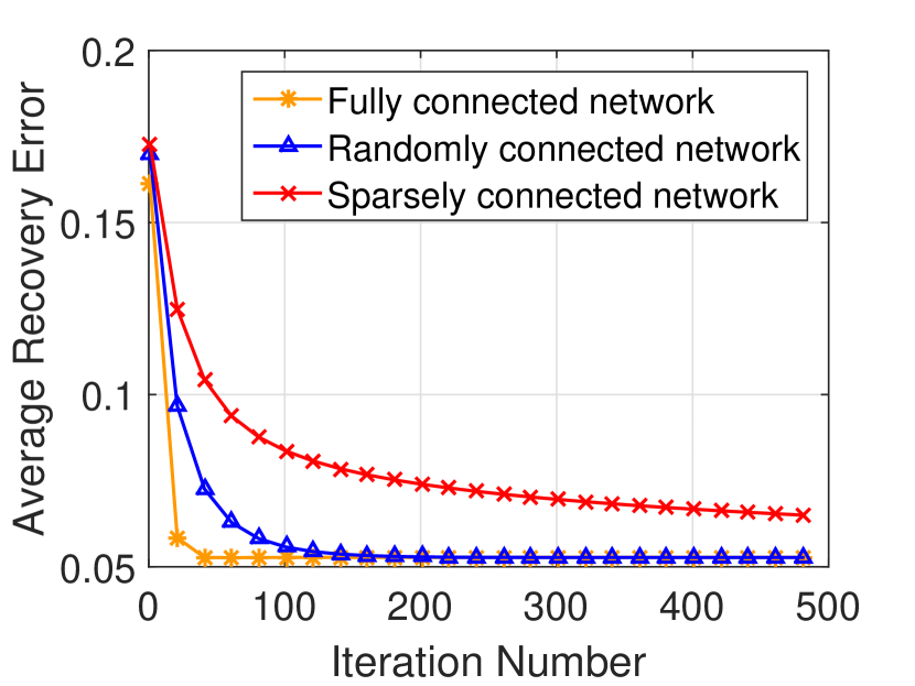
(a) Influence of the network topology on the convergence rate of CBGA-GMS

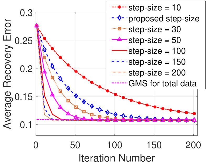
(b) Influence of different step-sizes on the convergence rate of CBGA-GMS

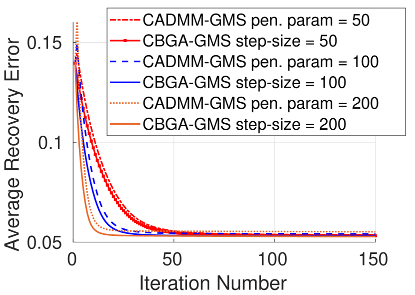
(c) CBGA-GMS vs CADMM-GMS

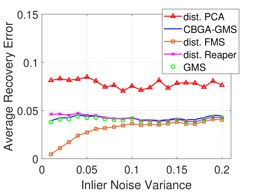
(d) Influence of inlier noise variance on distributed PCA, Reaper, GMS and FMS

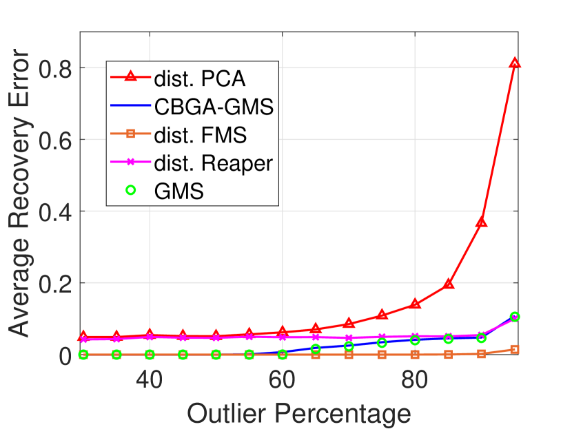
(e) Influence of outlier percentage on distributed PCA, Reaper, GMS, FMS; $\sigma=0$

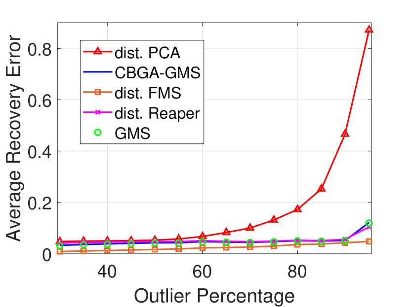
(f) Influence of outlier percentage on distributed PCA, Reaper, GMS, FMS; $\sigma=0.05$

Figure 2: Demonstration of properties of the distributed algorithms on synthetic data.

5.2.3 Comparing CBGA-GMS with CADMM-GMS

A CADMM scheme for GMS, which directly follows [23], is described in §A.3. It is referred to as CADMM-GMS. Both CBGA-GMS and CADMM-GMS are somewhat parallel and it follows from (17) and (24) that their corresponding parameters $\mu$ and $\rho$ play similar roles. We compare them using data generated from the model described in §5.1, where $K=5$, $D=50$, $d=3$, $\sigma=0.05$, $N^{0}=$5000$$ and $N^{1}=500$. We tested the following same values of $\rho$ and $\mu$: 50, 100 and 200. We remark that the $\mu$ proposed in (36) obtained the value 51.1. Since both algorithms performed similarly when using this value and 50, we did not report the performance with this value. Fig. 2(c) shows the recovery errors vs. the number of iterations for both algorithms with these step-sizes. We note that both algorithms converge with very similar speed, where CBGA-GMS converges slightly faster. For the smaller values of $\mu$ and $\rho$ (100 and 200) the algorithms achieve the same recovery error. However, for the larger value of the parameter (300), the recovery error of CADMM-GMS is slightly higher than the recovery error of CBGA-GMS.

5.2.4 Comparison of the Proposed Algorithms

We compare GMS, the $3$ proposed distributed RSR algorithms and distributed PCA in different settings and report the results in Figs. 2(d)-2(f). Fig. 2(d) demonstrates how the inlier noise variance $\sigma$ affects the convergence of the four methods. The data for this figure was created according to the model described in §5.1, where $D=50,$ $d=3,$ $K=5,$ $N^{0}=$3000$$, $N^{1}=$1000$$ and $\sigma$ varies between $0$ and $0.2$ with increments of $0.01.$ In this figure, for all tested values of $\sigma,$ CBGA-PCA performs the worst and distributed FMS performs the best, where CBGA-GMS and distributed Reaper are somewhat comparable.

Figs. 2(e) and 2(f) demonstrate the influence of the outlier percentage on the average recovery error of the four distributed methods and GMS (for the total data) with and without inlier noise. We generate data according to the model of §5.1, where $D=50,$ $d=3,$ $K=10,$ $\sigma=0$ for Fig. 2(e), $\sigma=0.5$ for Fig. 2(f), $N^{0}=$5000$$ and $N^{1}$ is chosen such that the outlier percentage in the total data varies between $30\%$ to $95\%$ with increments of $5\%$. For both cases ($\sigma=0$ and $\sigma=0.05$) and for all percentages of outliers, the recovery error for distributed FMS is the smallest one and that of CBGA-PCA is the largest one. Figs. 2(e) and 2(f) also demonstrate that when the data is corrupted with outliers (percentage of outliers higher than $65\%$), the distributed RSR algorithms perform significantly better than distributed PCA. For the case of $\sigma=0$, distributed FMS and CBGA-GMS succeed with exact recovery up to $90\%$ and $55\%$ of outliers respectively, whereas distributed Reaper could not exactly recover the subspace in the tested range.

In Figs. 2(d), 2(e) and 2(f), the recovery errors obtained by CBGA-GMS and GMS are comparable. We remark that the distributed implementations of PCA, Reaper and FMS also obtain similar recovery errors as the non-distributed ones in all of these experiments. However, since these figures are already dense, we do not report the results of the latter non-distributed implementations.

5.3 Real Data Experiments

Distributed RSR algorithms can be used as a preprocessing step for clustering, classification and regression. We apply our proposed distributed algorithms as a preprocessing step for two different tasks: linear regression, where we use the CTslices dataset $(N=$53500$,D=386)$ [22], and classification (multiclass SVM), where we use the Human Activity Recognition (HAR) dataset $(N=$10299$,D=561)$ [2, 22]. For both datasets we apply initial centering by the geometric median and to ensure full-rank data in all processors we reduce dimension to $D=150$ by distributed exact PCA (see §A.1). We remark that higher values of reduced dimensions $D$ were also possible. We report the results for one of the processors as they are the same for all of them.

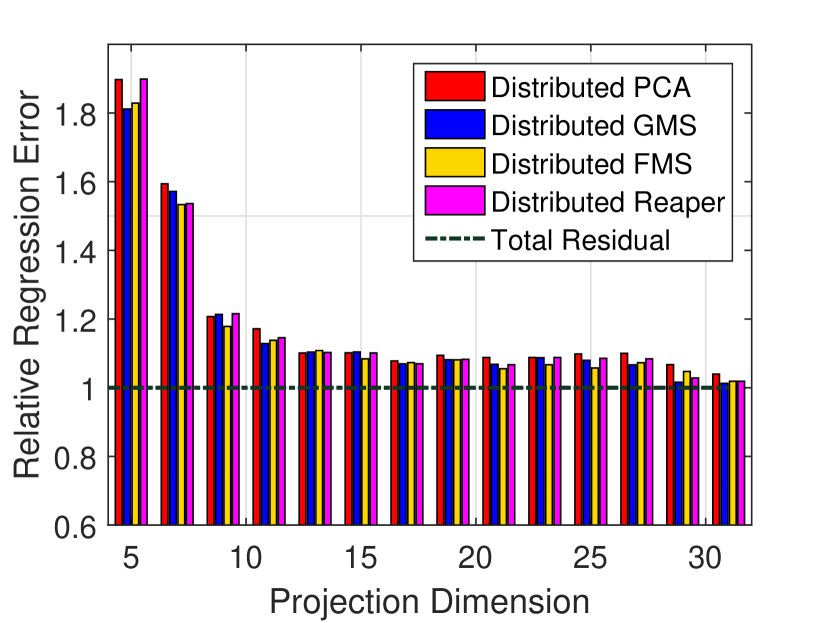
(a) CTslices

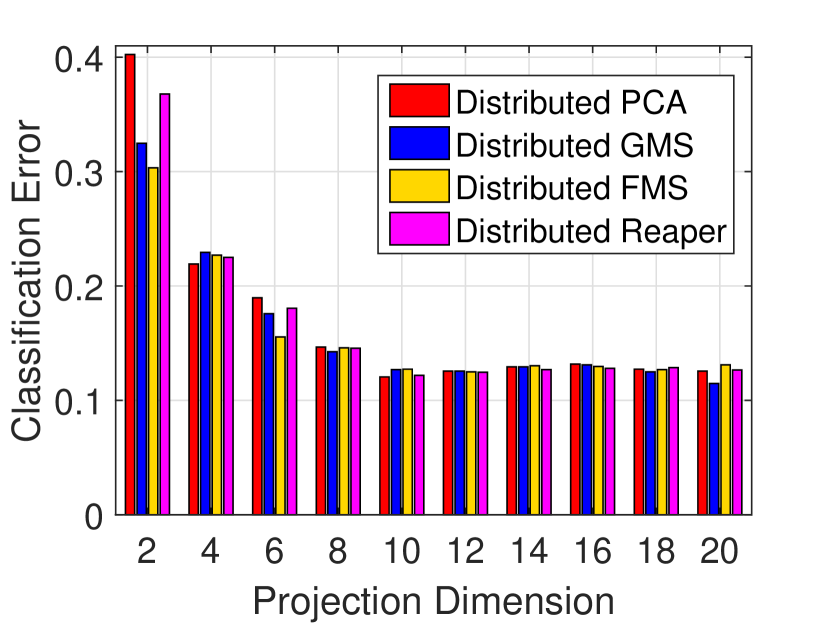
(b) Human Activity Recognition (HAR)

Figure 3: Demonstration of the proposed distributed algorithms on two real datasets: CTslices and HAR.

For the CTslices data, the algorithms are trained on $50000$ data points and tested on $3500$ data points. The training data is divided between $5$ processors, each containing $10000$ data points. We apply CBGA-PCA, CBGA-GMS, distributed FMS and distributed Reaper to reduce the dimension of the dataset to lie between $5$ and $30.$ We then apply linear least squares regression in the reduced dimension. Fig. 3(a) reports the relative regression error for the different projected dimensions. The relative regression error is the regression error for the data with the reduced dimension divided by the relative error for the data in $150$ dimensions. We notice that for almost all dimensions, the relative errors of distributed FMS and GMS are lower than those of distributed PCA, and the relative errors of distributed Reaper are either lower or comparable to those of distributed PCA.

For the HAR data, the algorithms are trained on $7352$ data points and tested on $2947$ data points. The training data is divided between $8$ processors, each containing $919$ data points. We apply CBGA-PCA, CBGA-GMS, distributed FMS and distributed Reaper to reduce the dimension of the dataset to lie between $2$ and $20.$ We then apply classification in the reduced dimensions. Fig. 3(b) reports classification error for the different projected dimensions. It demonstrates that in dimension $2,$ the distributed RSR algorithms, in particular, distributed FMS and GMS, have a clear advantage over distributed PCA. In other dimensions, distributed RSR algorithms perform at least as good as distributed PCA.

We comment that for all real datasets, the results of the distributed algorithms are very similar to those of the non-distributed ones. Differences between all distributed and non-distributed implementations may exist when the initial dimension $D$ is large and an initial dimension reduction by OSE is applied (see §A.1). An effect of OSE on the performance of PCA in a distributed setting is documented in [21].

Appendix A Solutions of Related Problems

We first use the idea of CBGA-GMS to solve two simpler problems: distributed computation of the PCA subspace and distributed computation of the geometric median. We then describe a CADMM solution for distributed GMS.

A.1 Distributed PCA for Arbitrarily Distributed Network

Before describing the CBGA procedure for PCA, we remark that if the dimension $D$ is not high, then the following simple procedure can be applied to solve the problem. One may propagate the local covariance matrices among the network and recover the exact covariance matrix at each processor and use it for PCA computation. We refer to it as exact distributed PCA. If the dimension $D$ is high, then it can be reduced by an OSE procedure described below before applying the exact distributed PCA algorithm.

Our proposed CBGA-PCA algorithm is similar to [1, 35, 5], but uses instead the PCA formulation in (7). This formulation leads to a direct solution of the local optimization problem. In order to apply (7), one needs to guarantee that for all $1\leq k\leq K$, $\mathcal{X}_{k}$ has full rank. If $\mathcal{X}_{k}$ is rank-deficient, one can reduce its dimension. If the dimension $D$ is high, one can sample an Oblivious Subspace Embedding (OSE) matrix $\boldsymbol{H}$ [32] and instead of $\mathcal{X}_{k}$ consider $\boldsymbol{H}\mathcal{X}_{k}$. One common OSE $\boldsymbol{H}$ has only one non-zero entry per row. By taking an appropriate number of rows for $\boldsymbol{H}$, one can assume that the projected data at each node has full rank. If the dimension $D$ is not high, then the exact distributed PCA, or a faster approximate version of it, can be used to reduce the dimension.

Next, we clarify the application of CBGA to (7). In view of §2, it is sufficient to compute the dual function of (7) at each node, that is, compute for each $1\leq k\leq K$:

(20) $$d_{k}(\boldsymbol{\Lambda})=\min\limits_{\boldsymbol{Q}\in\mathbb{H}}\left(\sum\limits_{\boldsymbol{x}\in\mathcal{X}_{k}}\|\boldsymbol{Q}\boldsymbol{x}\|^{2}+\operatorname{tr}(\boldsymbol{A}_{k}\boldsymbol{Q})\right),\text{ where }\boldsymbol{A}_{k}=\sum\limits_{m\in\mathcal{E}_{k}}c_{mk}\boldsymbol{\Lambda}_{m}^{T}.$$

Appendix B.1 guarantees the unique minimizer of (20) and explains how to find it.

Since the minimized function in (7) is strongly convex, it follows from [17] that its dual function $d(\boldsymbol{\Lambda})=\sum_{k=1}^{K}d_{k}(\boldsymbol{\Lambda})$, where $d_{k}(\boldsymbol{\Lambda})$ is defined in (20), is Lipschitz smooth. This implies that the CBGA algorithm for PCA converges to the PCA solution for the total data with rate $O(1/t).$ The complexity of CBGA-PCA is $O(T_{CBGA}\times N_{\max}\times D^{2})$ (see §B.1.3). This algorithm is not optimal in terms of complexity and communication. Indeed, the distributed exact PCA algorithm described above is simpler and achieves the exact PCA subspace. Nevertheless, we find this CBGA-PCA interesting for two reasons. First of all, it is similar to previous attempts [1, 35, 5] that did not clarify how to solve the local dual problem. Second of all, CBGA-PCA simply demonstrates the main idea of the more complicated CBGA-GMS procedure.

A.2 Distributed Geometric Median

The geometric median of a discrete dataset $\mathcal{X}\subset\mathbb{R}^{D}$ is defined as

(21) $$\operatorname*{arg\,min}\limits_{\boldsymbol{y}\in\mathbb{R}^{D}}\sum\limits_{\boldsymbol{x}\in\mathcal{X}}\|\boldsymbol{x}-\boldsymbol{y}\|.$$

Weiszfeld’s algorithm [36] is a common numerical approach to approximating (21) within a sufficiently small error. It applies an iteratively reweighted least squares (IRLS) procedure. However, if in one of the iterations, the estimate coincides with one of the data points, then Weiszfeld’s algorithm fails to converge to the geometric median. To avoid this issue, we consider the following regularized version of (21):

(22) $$\operatorname*{arg\,min}\limits_{\boldsymbol{y}\in\mathbb{R}^{D}}\sum\limits_{\boldsymbol{x}\in\mathcal{X},\|\boldsymbol{x}-\boldsymbol{y}\|\geq\delta}\|\boldsymbol{x}-\boldsymbol{y}\|+\sum\limits_{\boldsymbol{x}\in\mathcal{X},\|\boldsymbol{x}-\boldsymbol{y}\|<\delta}\left(\frac{\|\boldsymbol{x}-\boldsymbol{y}\|^{2}}{2\delta}+\frac{\delta}{2}\right),$$

where $\delta>0$ is a small regularization parameter. We can solve (22) by the generalized Weiszfeld’s algorithm [10, §4]. This algorithm runs as follows: it starts with an initial guess $\boldsymbol{y}_{0}\in\mathbb{R}^{D},$ and at iteration $s\geq 1$ it computes

$$\boldsymbol{y}_{s}=\sum\limits_{\boldsymbol{x}\in\mathcal{X}}\frac{\boldsymbol{x}}{\max\left(\|\boldsymbol{x}-\boldsymbol{y}_{s-1}\|,\delta\right)}\biggm{/}\sum\limits_{\boldsymbol{x}\in\mathcal{X}}\frac{1}{\max\left(\|\boldsymbol{x}-\boldsymbol{y}_{s-1}\|,\delta\right)}.$$

The sequence $\{\boldsymbol{y}_{s}\}_{s\in\mathbb{N}}$ $r$-linearly converges to the solution of (22) (see [10]).

We assume a dataset $\mathcal{X}$ with $\{\mathcal{X}_{k}\}_{k=1}^{K}$ distributed at $K$ nodes, and distributedly compute the regularized geometric median of $\mathcal{X}$ by CBGA. In view of §2, it is enough to compute the dual function of (22) at each node, that is, compute for each $1\leq k\leq K$

(23) $$d_{k}(\boldsymbol{\lambda})=\min\limits_{\boldsymbol{y}\in\mathbb{R}^{D}}\sum\limits_{\begin{subarray}{c}\boldsymbol{x}\in\mathcal{X}_{k},\\ \|\boldsymbol{x}-\boldsymbol{y}\|\geq\delta\end{subarray}}\|\boldsymbol{x}-\boldsymbol{y}\|+\sum\limits_{\begin{subarray}{c}\boldsymbol{x}\in\mathcal{X}_{k},\\ \|\boldsymbol{x}-\boldsymbol{y}\|<\delta\end{subarray}}\left(\frac{\|\boldsymbol{x}-\boldsymbol{y}\|^{2}}{2\delta}+\frac{\delta}{2}\right)+\sum_{m\in\mathcal{E}_{k}}c_{mk}\boldsymbol{\lambda}_{m}^{T}\boldsymbol{y},$$

where $\boldsymbol{\lambda}=[\boldsymbol{\lambda}_{1}^{T},\dots,\boldsymbol{\lambda}_{M}^{T}]^{T}\in\mathbb{R}^{MD}.$ We suggest solving (23) by IRLS as follows: start with an initial guess $\boldsymbol{y}_{k}^{0}\in\mathbb{R}^{D}$ and at iteration $s\geq 1$ compute

$$\boldsymbol{y}_{k}^{s}=\left(2\sum\limits_{\boldsymbol{x}\in\mathcal{X}_{k}}\frac{\boldsymbol{x}}{\max\left(\|\boldsymbol{x}-\boldsymbol{y}_{k}^{s-1}\|,\delta\right)}-\sum_{m\in\mathcal{E}_{k}}c_{mk}\boldsymbol{\lambda}_{m}\right)\biggm{/}\left(2\sum\limits_{\boldsymbol{x}\in\mathcal{X}_{k}}\frac{1}{\left(\|\boldsymbol{x}-\boldsymbol{y}_{k}^{s-1}\|,\delta\right)}\right).$$

The convergence of $\{\boldsymbol{y}_{k}^{s}\}_{s\in\mathbb{N}}$ follows from that of IRLS (see [10]) and CBGA (see §2).

A.3 CADMM Solution for the Distributed GMS Problem

We formulate in Algorithm 3 a CADMM solution of the distributed GMS problem by following the CADMM scheme of [23]. The solution of the local problem is discussed in §A.3.1.

Algorithm 3 CADMM implementation for distributed GMS (CADMM-GMS)

  Input: Network with $K$ nodes, $\mathcal{X}_{1},\dots,\mathcal{X}_{K}:$ datasets in the $K$ nodes, $T_{CADMM}$, $T_{GMS}$: stopping iteration numbers, $\delta$: regularization parameter (default: $10^{-10}$) and $\rho$: penalty parameter for CADMM

  Set: For all $1\leq k\leq K$, $\boldsymbol{Z}_{k}^{0}=\boldsymbol{0}$ and $\boldsymbol{Q}_{k}^{0}$ is the solution of Algorithm 1 with input $\mathcal{X}_{k},$ $\boldsymbol{A}_{k}=\boldsymbol{0},$ $T_{GMS}$ and $\delta$

  for $s=1:T_{CADMM}$ do

     

• For $1\leq k\leq K$ update $\boldsymbol{Z}_{k}^{s}$ by

  (24) $$\boldsymbol{Z}_{k}^{s}=\boldsymbol{Z}_{k}^{s-1}+\rho\sum_{j\in\mathcal{N}_{k}}\left(\boldsymbol{Q}_{k}^{s-1}-\boldsymbol{Q}_{j}^{s-1}\right)$$

• For $1\leq k\leq K$ apply the algorithm described in §A.3.1 to solve

  (25) $$\boldsymbol{Q}_{k}^{s}=\operatorname*{arg\,min}\limits_{\boldsymbol{Q}_{k}\in\mathbb{H}}\tilde{G}_{ADMM}(\boldsymbol{Q}_{k}),\text{ where }$$

  $\tilde{G}_{ADMM}(\boldsymbol{Q}_{k})=F_{k}(\boldsymbol{Q}_{k})+\operatorname{tr}\left(\boldsymbol{Q}_{k}^{T}\boldsymbol{Z}_{k}^{s}\right)+\rho\sum\limits_{j\in\mathcal{N}_{k}}\left\|\boldsymbol{Q}_{k}-\frac{\boldsymbol{Q}_{k}^{(s-1)}+\boldsymbol{Q}_{j}^{(s-1)}}{2}\right\|_{2}^{2}$

  end for

  return  $L_{k}:=$ the span of the bottom $d$ eigenvectors of $\boldsymbol{Q}_{k}^{T_{CADMM}},1\leq k\leq K$

A.3.1 Algorithm for computing the solution of (25)

We propose an iterative scheme for solving (25), which is almost identical to Algorithm 1, but at each iteration $s$ instead of finding the trace one solution of (14), it finds the trace one solution of the following Lyapunov equation in $\boldsymbol{P}$:

(26) $$\boldsymbol{P}\left(\sum\limits_{\boldsymbol{x}\in\mathcal{X}_{k}}\frac{\boldsymbol{x}\boldsymbol{x}^{T}}{2\max(\|\boldsymbol{Q}\boldsymbol{x}\|,\delta)}+\rho|\mathcal{N}_{k}|\boldsymbol{I}\right)+\left(\sum\limits_{\boldsymbol{x}\in\mathcal{X}_{k}}\frac{\boldsymbol{x}\boldsymbol{x}^{T}}{2\max(\|\boldsymbol{Q}\boldsymbol{x}\|,\delta)}+\rho|\mathcal{N}_{k}|\boldsymbol{I}\right)\boldsymbol{P}\\ +\boldsymbol{Z}_{k}^{s}-\rho\sum_{j\in\mathcal{N}_{k}}\left(\boldsymbol{Q}_{k}^{s-1}+\boldsymbol{Q}_{j}^{s-1}\right)=c\boldsymbol{I}.$$

Here, $c$ is chosen so that $\operatorname{tr}(\boldsymbol{P})=1$ and its existence is guaranteed by Lemma B.2. The convergence theory for this iterative algorithm is the same as the one developed for Algorithm 1.

Appendix B Supplementary Details

B.1 On the Minimizer of (20)

We first state the main result of this section:

Lemma B.1.

If $\mathcal{X}_{k}\subset\mathbb{R}^{D}$ is full rank and $\boldsymbol{A}_{k}\in\mathcal{S}^{D}$, then the minimizer of (20) is unique. Furthermore, there exists a unique $c^{\prime}\in\mathbb{R}$ such that this minimizer is the unique solution of the following equation with $c=c^{\prime}$

(27) $$\boldsymbol{Q}\left(\sum\limits_{\boldsymbol{x}\in\mathcal{X}_{k}}\boldsymbol{x}\boldsymbol{x}^{T}\right)+\left(\sum\limits_{\boldsymbol{x}\in\mathcal{X}_{k}}\boldsymbol{x}\boldsymbol{x}^{T}\right)\boldsymbol{Q}+\boldsymbol{A}_{k}=c\boldsymbol{I}.$$

Section B.1.1 states and proves a lemma about the solution of the above Lyapunov equation and §B.1.2 then uses this latter lemma to conclude Lemma B.1. At last, §B.1.3 briefly discusses the computation of the minimizer of (20).

B.1.1 Preliminary lemma

We verify the following lemma.

Lemma B.2.

If $c\in\mathbb{R},$ $\boldsymbol{X}\in\mathcal{S}_{++}^{D}$ and $\boldsymbol{A}\in\mathcal{S}^{D}$, then the following Lyapunov equation

(28) $$\boldsymbol{Q}\boldsymbol{X}+\boldsymbol{X}\boldsymbol{Q}+\boldsymbol{A}=c\boldsymbol{I}$$

has a unique solution in $\boldsymbol{Q}\in\mathcal{S}^{D}$. Furthermore, $\operatorname{tr}(\boldsymbol{Q})$ is an increasing linear function of $c$ with slope $\operatorname{tr}(\boldsymbol{X}^{-1})/2.$

Proof B.3.

The existence and uniqueness of the solution of (28) is well-known [7, page 107]. We thus only need to show that $\operatorname{tr}(\boldsymbol{Q})$ is an increasing linear function of $c$. Assume that $\boldsymbol{Q}_{1}$ and $\boldsymbol{Q}_{2}$ are the solutions of (28) corresponding to $c_{1}$ and $c_{2},$ that is,

(29) $$\boldsymbol{Q}_{1}\boldsymbol{X}+\boldsymbol{X}\boldsymbol{Q}_{1}+\boldsymbol{A}=c_{1}\boldsymbol{I}\text{ and }\boldsymbol{Q}_{2}\boldsymbol{X}+\boldsymbol{X}\boldsymbol{Q}_{2}+\boldsymbol{A}=c_{2}\boldsymbol{I}.$$

Subtracting the two equations in (29), results in

(30) $$(\boldsymbol{Q}_{1}-\boldsymbol{Q}_{2})\boldsymbol{X}+\boldsymbol{X}(\boldsymbol{Q}_{1}-\boldsymbol{Q}_{2})=(c_{1}-c_{2})\boldsymbol{I},$$

whose unique solution is $(\boldsymbol{Q}_{1}-\boldsymbol{Q}_{2})=(c_{1}-c_{2})\boldsymbol{X}^{-1}/2$. By taking traces of both sides of the solution, we get that $(\operatorname{tr}(\boldsymbol{Q}_{1})-\operatorname{tr}(\boldsymbol{Q}_{2}))/(c_{1}-c_{2})=\operatorname{tr}(\boldsymbol{X}^{-1})/2>0$.

B.1.2 Proof of Lemma B.1

Since $\mathcal{X}_{k}$ is full rank, $\sum_{\boldsymbol{x}\in\mathcal{X}_{k}}\boldsymbol{x}\boldsymbol{x}^{T}\in\mathcal{S}_{++}^{D}.$ Hence the minimized function in (20) is strongly convex and its minimizer is unique.

We note that (27) is a Lyapunov equation in $\boldsymbol{Q}.$ Lemma B.2 implies that there is a unique value $c^{\prime}$ for which the unique solution of (27) has trace $1.$ We denote this solution by $\boldsymbol{Q}^{\prime}.$ Next, we show that $\boldsymbol{Q}^{\prime}$ is the minimizer of (20). The following two facts: $\sum_{\boldsymbol{x}\in\mathcal{X}_{k}}\|\boldsymbol{Q}\boldsymbol{x}_{k}\|^{2}+\operatorname{tr}(\boldsymbol{A}_{k}\boldsymbol{Q})=\sum_{\boldsymbol{x}\in\mathcal{X}_{k}}\operatorname{tr}(\boldsymbol{Q}\boldsymbol{x}_{k}\boldsymbol{x}_{k}^{T}\boldsymbol{Q})+\operatorname{tr}(\boldsymbol{A}_{k}\boldsymbol{Q})$ for $\boldsymbol{Q}\in\mathbb{H}$ and $\operatorname{tr}(\boldsymbol{Q})=1$ for $\boldsymbol{Q}\in\mathbb{H},$ imply the same minimizer for (20) and

(31) $$\min_{\boldsymbol{Q}\in\mathbb{H}}l(\boldsymbol{Q}),\text{ where }l(\boldsymbol{Q})=\sum_{\boldsymbol{x}\in\mathcal{X}_{k}}\operatorname{tr}(\boldsymbol{Q}\boldsymbol{x}_{k}\boldsymbol{x}_{k}^{T}\boldsymbol{Q})+\operatorname{tr}(\boldsymbol{A}_{k}\boldsymbol{Q})-c^{\prime}\operatorname{tr}(\boldsymbol{Q}).$$

Since $l(\boldsymbol{Q})$ is convex on $\mathbb{H}$, we conclude that $\boldsymbol{Q}^{\prime}$ minimizes (31) by showing that the derivative of $l(\boldsymbol{Q})$ at $\boldsymbol{Q}^{\prime}$, when restricted to $\mathbb{H}$, is $\boldsymbol{0}$:

$$\square \frac{d}{d\boldsymbol{Q}}l(\boldsymbol{Q})\biggr{|}_{\boldsymbol{Q}=\boldsymbol{Q}^{\prime}}=\boldsymbol{Q}^{\prime}\left(\sum_{\boldsymbol{x}\in\mathcal{X}_{k}}\boldsymbol{x}\boldsymbol{x}^{T}\right)+\left(\sum_{\boldsymbol{x}\in\mathcal{X}_{k}}\boldsymbol{x}\boldsymbol{x}^{T}\right)\boldsymbol{Q}^{\prime}+\boldsymbol{A}_{k}-c^{\prime}\boldsymbol{I}=\boldsymbol{0}.$$

B.1.3 Computing the Minimizer of (20)

In view of Lemma B.2 we compute $c^{\prime}$ and the corresponding solution of (29) as follows. We solve (27) with $c=0$ to obtain $\boldsymbol{Q}_{*}\in\mathcal{S}^{D}$. We then use $\operatorname{tr}(\boldsymbol{Q}_{*})$ and the slope $\operatorname{tr}(\boldsymbol{X}^{-1})/2$, where $\boldsymbol{X}=\sum_{\boldsymbol{x}\in\mathcal{X}_{k}}\boldsymbol{x}\boldsymbol{x}^{T}$, to find $c^{\prime}$. Therefore, computing this minimizer requires computing $\boldsymbol{X}$, which costs $O(N_{\max}\times D^{2})$, and solving two Lyapunov equations, which costs $O(D^{3})$ (see [4]).

B.2 Proof of Eq. 15

Let $\boldsymbol{X}=\sum_{i=1}^{N}\boldsymbol{x}_{i}\boldsymbol{x}_{i}^{T}/\left(2\max(\|\boldsymbol{Q}\boldsymbol{x}_{i}\|,\delta)\right)$ and note that $\boldsymbol{X}\in\mathcal{S}_{++}^{D}$. This observation and Lemma B.2 imply that there is a unique value $c\in\mathbb{R}$ for which (14) has a unique solution in $\mathbb{H}$. We will show that $c>\lambda_{1}(\boldsymbol{A})$, equivalently $\boldsymbol{A}-c\boldsymbol{I}\preceq\boldsymbol{0}$, and thus in view of [7, page 107], this solution is in $\mathcal{S}_{++}^{D}$.

To get this estimate, we rewrite (14) as $\boldsymbol{P}+\boldsymbol{X}\boldsymbol{P}\boldsymbol{X}^{-1}+\boldsymbol{A}\boldsymbol{X}^{-1}=c\boldsymbol{X}^{-1}.$ Applying trace to both sides and using the following facts: $\operatorname{tr}(\boldsymbol{P})=1,$ $\operatorname{tr}(\boldsymbol{X}\boldsymbol{P}\boldsymbol{X}^{-1})=\operatorname{tr}(\boldsymbol{X}^{-1}\boldsymbol{X}\boldsymbol{P})=1$ and $\operatorname{tr}(\boldsymbol{A}\boldsymbol{X}^{-1})\geq\lambda_{D}(\boldsymbol{A})\operatorname{tr}(\boldsymbol{X}^{-1})$ yields $c\geq 2/\operatorname{tr}(\boldsymbol{X}^{-1})+\lambda_{D}(\boldsymbol{A}).$

Let $\boldsymbol{X}_{*}=\sum_{i=1}^{N}\boldsymbol{x}_{i}\boldsymbol{x}_{i}^{T}/\left(2\max(\|\boldsymbol{x}_{i}\|,\delta)\right).$ Since $\boldsymbol{Q}\in\mathcal{S}_{+}^{D}\cap\mathbb{H}$ and $\max(\|\boldsymbol{Q}\boldsymbol{x}_{i}\|,\delta)\leq\max(\|\boldsymbol{x}_{i}\|,\delta)$ for $1\leq i\leq N,$ $\boldsymbol{X}-\boldsymbol{X}_{*}\in\mathcal{S}_{+}^{D},$ which implies that $\boldsymbol{X}_{*}^{-1}-\boldsymbol{X}^{-1}\in\mathcal{S}_{+}^{D}.$ Combining the last result with (13), $\|\boldsymbol{A}\|_{2}>\lambda_{1}(-A)$ and the estimate of $c$ we obtain that $c\geq 2/\operatorname{tr}(\boldsymbol{X}_{*}^{-1})+\lambda_{D}(\boldsymbol{A})\geq 2\|\boldsymbol{A}\|_{2}-\lambda_{1}(-\boldsymbol{A})\geq\lambda_{1}(\boldsymbol{A}).$

The last statement of the lemma is a direct application of Lemma B.2. $\square$

B.3 On the Choice of the Step-Size

In view of Eq. 15, we require that condition (13) holds at each iteration of Algorithm 2 and each node $k$. The following lemma shows that a choice of a sufficiently small step-size $\mu$ guarantees this requirement. After verifying this lemma, we discuss weaker restrictions on the step-size as well as a weaker practical version of condition (13).

Lemma B.4.

If $\{\mathcal{X}_{k}\}_{k=1}^{K}\subset\mathbb{R}^{D}$ are datasets distributed at $K$ nodes, $n\in\mathbb{N}$ and

(32) $$\mu\leq\frac{1}{n\cdot\max\limits_{1\leq k\leq K}|\mathcal{E}_{k}|\cdot\operatorname{tr}\left(\left(\sum\limits_{x\in\mathcal{X}_{k}}\frac{\boldsymbol{x}\boldsymbol{x}^{T}}{\max(\|\boldsymbol{x}\|,\delta)}\right)^{-1}\right)},$$

then at each iteration $s\leq n$ of Algorithm 2 and node $k$, $\boldsymbol{A}_{k}^{s}$ satisfies condition (13).

Proof B.5.

We estimate the LHS of (13) at iteration $s$ as follows:

(33) $$\|\boldsymbol{A}_{k}^{s}\|_{2}=\left\|\sum\limits_{m\in\mathcal{E}_{k}}c_{mk}\boldsymbol{\Lambda}_{m}^{s}\right\|_{2}\leq\sum\limits_{m\in\mathcal{E}_{k}}\|\boldsymbol{\Lambda}_{m}^{s}\|_{2}.$$

In order to evaluate $\|\boldsymbol{\Lambda}_{m}^{s}\|_{2}$ for $1\leq m\leq M,$ we apply (16) and basic inequalities:

(34) $$\|\boldsymbol{\Lambda}_{m}^{s}\|_{2}=\|\boldsymbol{\Lambda}_{m}^{s-1}+\mu(c_{mk}\boldsymbol{Q}_{k}^{s}-c_{mk}\boldsymbol{Q}_{q}^{s})\|_{2}\leq\|\boldsymbol{\Lambda}_{m}^{s-1}\|_{2}+\mu\|\boldsymbol{Q}_{k}^{s}-\boldsymbol{Q}_{q}^{s}\|_{2}\leq\\ \|\boldsymbol{\Lambda}_{m}^{s-1}\|_{2}+\mu\max\{\|\boldsymbol{Q}_{k}^{s}\|_{2},\|\boldsymbol{Q}_{q}^{s}\|_{2}\}\leq\|\boldsymbol{\Lambda}_{m}^{s-1}\|_{2}+\mu\leq\dots\leq s\mu\leq n\mu.$$

Combining (32), (33) and (34) results in

(35) $$\|\boldsymbol{A}_{k}^{s}\|_{2}\leq\sum\limits_{m\in\mathcal{E}_{k}}\|\boldsymbol{\Lambda}_{m}^{s}\|_{2}\leq|\mathcal{E}_{k}|n\mu\leq 1\biggr{/}\operatorname{tr}\left(\left(\sum\limits_{\boldsymbol{x}\in\mathcal{X}}\frac{\boldsymbol{x}\boldsymbol{x}^{T}}{2\max(\|\boldsymbol{x}\|,\delta)}\right)^{-1}\right).$$

In practice one may apply several iterations with the same fixed step-size and gradually reduce it until it satisfies the estimate above. Nevertheless, this estimate represents a worse-case scenario and typically we expect an improved one. Indeed, first note that condition (13) represents a worse-case scenario. In the proof of Eq. 15 we used the worst-case estimate $\|\boldsymbol{Q}\|\leq 1$. However, typically $\|\boldsymbol{Q}\|\sim 1/D$. This will introduce a multiplicative factor $D$ for the RHS of (13) and thus of (32). Second, in (34) we used the estimate $\|\boldsymbol{Q}^{s}_{k}-\boldsymbol{Q}^{s}_{q}\|\leq\max\{\|\boldsymbol{Q}_{k}^{s}\|_{2},\|\boldsymbol{Q}_{q}^{s}\|_{2}\}\leq 1.$ However, typically for $\boldsymbol{Q}^{s}_{k},\boldsymbol{Q}^{s}_{q}\in\mathbb{H}\cap\mathcal{S}_{++}^{D},$ $\max\{\|\boldsymbol{Q}_{k}^{s}\|_{2},\|\boldsymbol{Q}_{q}^{s}\|_{2}\}\sim 1/D.$ This observation introduces another multiplicative factor $D$ for the RHS of (32). These two observations suggest, in practice, the following choice of a step-size:

(36) $$\mu=\frac{D^{2}}{n\cdot\max\limits_{1\leq k\leq K}|\mathcal{E}_{k}|\cdot\operatorname{tr}\left(\left(\sum\limits_{x\in\mathcal{X}_{k}}\frac{\boldsymbol{x}\boldsymbol{x}^{T}}{\max(\|\boldsymbol{x}\|,\delta)}\right)^{-1}\right)}.$$

Third of all, we note that for sufficiently small step-sizes the gradient descent gets closer to the solution, that is, $\|\boldsymbol{Q}_{k}^{s}-\boldsymbol{Q}_{q}^{s}\|_{2}\to 0,$ for $1\leq k,q\leq K$. However, we used $1/D$ as an upper bound for $\|\boldsymbol{Q}_{k}^{s}-\boldsymbol{Q}_{q}^{s}\|_{2}.$ At last, we comment that while the above analysis aims to guarantee that at each iteration the solution is in $\mathbb{H}\cap\mathcal{S}_{++}^{D}$ (since (13) guarantees this), in practice it is not a main concern for small step-sizes and large number of iterations. Indeed, the solution of (4) coincides with the solution of GMS for the total data, which is in $\mathbb{H}\cap\mathcal{S}_{++}^{D}$. Thus, by choosing the step-size small enough we will always converge to the solution.

B.4 Proof of Theorem 1

We establish an auxiliary lemma in §B.4.1 and conclude Theorem 1 in §B.4.2 by following ideas of [10, 37] and using this lemma.

B.4.1 Preliminary Proposition

We first apply Lemma B.2 to define the mapping $T_{\boldsymbol{A}}(\boldsymbol{Q})$ and then establish the continuity of $T_{\boldsymbol{A}}(\boldsymbol{Q})$ in $\mathcal{S}_{++}^{D}.$

Definition 2 (The mapping $T_{\boldsymbol{A}}(\boldsymbol{Q})$).

If $\{\boldsymbol{x}_{i}\}_{i=1}^{N}\subset\mathbb{R}^{D},$ $\delta>0,$ $\boldsymbol{Q}\in\mathcal{S}_{+}^{D}\cap\mathbb{H}$ and $\boldsymbol{A}\in\mathcal{S}^{D}$ with $\operatorname{tr}(\boldsymbol{A})=0,$ then $T_{\boldsymbol{A}}(\boldsymbol{Q})$ is the solution of the following equation in $\boldsymbol{P}$

(37) $$\boldsymbol{P}\left(\sum\limits_{i=1}^{N}\frac{\boldsymbol{x}_{i}\boldsymbol{x}_{i}^{T}}{\max(\|\boldsymbol{Q}\boldsymbol{x}_{i}\|,\delta)}\right)+\left(\sum\limits_{i=1}^{N}\frac{\boldsymbol{x}_{i}\boldsymbol{x}_{i}^{T}}{\max(\|\boldsymbol{Q}\boldsymbol{x}_{i}\|,\delta)}\right)\boldsymbol{P}+\boldsymbol{A}=c\boldsymbol{I},$$

where $c=c(\boldsymbol{Q})\in\mathbb{R}$ is uniquely chosen so that the solution has trace 1.

Lemma B.6.

Assume a sequence $\{\boldsymbol{Q}^{t}\}_{t\in\mathbb{N}}\subset\mathcal{S}_{++}^{D}\cap\mathbb{H}$, $\boldsymbol{A}\in\mathcal{S}^{D}$ with $\operatorname{tr}(\boldsymbol{A})=0,$ $\{\boldsymbol{x}_{i}\}_{i=1}^{N}\subset\mathbb{R}^{D}$ and $\delta>0.$ If $\boldsymbol{Q}^{t}\to\hat{\boldsymbol{Q}},$ then $T_{\boldsymbol{A}}(\boldsymbol{Q}^{t})\to T_{\boldsymbol{A}}(\hat{\boldsymbol{Q}}).$

Proof B.7.

For $t\in\mathbb{N},$ let $\boldsymbol{P}^{t}=T_{\boldsymbol{A}}(\boldsymbol{Q}^{t})$ be the trace one solution of (37) with $\boldsymbol{Q}=\boldsymbol{Q}^{t}$ and $c=c^{t}.$ Let $\hat{\boldsymbol{P}}=T_{\boldsymbol{A}}(\hat{\boldsymbol{Q}})$ be the trace one solution of (37) with $\boldsymbol{Q}=\hat{\boldsymbol{Q}}$ and $c=\hat{c}$. We need to prove that $\boldsymbol{P}^{t}\to\hat{\boldsymbol{P}}$ as $t\to\infty$. We write (37) with $\boldsymbol{P}^{t},\boldsymbol{Q}^{t}$ and $c^{t}$ as

(38) $$\boldsymbol{P}^{t}\left(\sum\limits_{i=1}^{N}\frac{\boldsymbol{x}_{i}\boldsymbol{x}_{i}^{T}}{\max(\|\boldsymbol{Q}^{t}\boldsymbol{x}_{i}\|,\delta)}\right)+\left(\sum\limits_{i=1}^{N}\frac{\boldsymbol{x}_{i}\boldsymbol{x}_{i}^{T}}{\max(\|\boldsymbol{Q}^{t}\boldsymbol{x}_{i}\|,\delta)}\right)\boldsymbol{P}^{t}+\boldsymbol{A}=c^{t}\boldsymbol{I}.$$

Note that $\boldsymbol{R}^{t}:=\sum_{i=1}^{N}\boldsymbol{x}_{i}\boldsymbol{x}_{i}^{T}/\max(\|\boldsymbol{Q}^{t}\boldsymbol{x}_{i}\|,\delta)\to\hat{\boldsymbol{R}}:=\sum_{i=1}^{N}\boldsymbol{x}_{i}\boldsymbol{x}_{i}^{T}/\max(\|\boldsymbol{Q}\boldsymbol{x}_{i}\|,\delta)$ as $t\to\infty$. Also observe that for $\boldsymbol{Q}=\hat{\boldsymbol{Q}},$ $c=\hat{c}$ and $T_{\boldsymbol{A}}(\boldsymbol{Q}^{t})=\boldsymbol{P}^{t}$, (37) has the form

(39) $$\boldsymbol{P}^{t}\boldsymbol{R}^{t}+\boldsymbol{R}^{t}\boldsymbol{P}^{t}+\boldsymbol{A}=c^{t}\boldsymbol{I}.$$

By subtracting $c^{t}\boldsymbol{I}$ from both sides of (39) and rewriting $c^{t}\boldsymbol{I}=c^{t}{\boldsymbol{R}^{t}}^{-1}\boldsymbol{R}^{t}/2+\boldsymbol{R}^{t}c^{t}{\boldsymbol{R}^{t}}^{-1}/2$, (39) becomes $(\boldsymbol{P}^{t}-c^{t}{\boldsymbol{R}^{t}}^{-1}/2)\boldsymbol{R}^{t}+\boldsymbol{R}^{t}(\boldsymbol{P}^{t}-c^{t}{\boldsymbol{R}^{t}}^{-1}/2)+\boldsymbol{A}=\boldsymbol{0}$. Similarly, $(\hat{\boldsymbol{P}}-\hat{c}{\hat{\boldsymbol{R}}}^{-1}/2)\hat{\boldsymbol{R}}+\hat{\boldsymbol{R}}(\hat{\boldsymbol{P}}-\hat{c}{\hat{\boldsymbol{R}}}^{-1}/2)+\boldsymbol{A}=\boldsymbol{0}$. Since $\boldsymbol{A}$ is fixed and $\boldsymbol{R}^{t}\to\hat{\boldsymbol{R}}$ as $t\to\infty,$ it follows from the last two expressions that

(40) $$\boldsymbol{P}^{t}-c^{t}{\boldsymbol{R}^{t}}^{-1}/2\to\hat{\boldsymbol{P}}-\hat{c}{\hat{\boldsymbol{R}}}^{-1}/2\text{ as }t\to\infty.$$

By taking the trace of both sides of (40) and using the facts that $\operatorname{tr}(\boldsymbol{P}^{t})=\operatorname{tr}(\hat{\boldsymbol{P}})=1$ and $\hat{\boldsymbol{R}}^{t}\to\boldsymbol{R}$ as $t\to\infty$, we get that $c^{t}\to\hat{c}$ and consequently $\boldsymbol{P}^{t}\to\hat{\boldsymbol{P}}$ as $t\to\infty.$

B.4.2 Conclusion of Theorem 1

We divide the proof of Theorem 1 into the following steps suggested in [37].

Step 1: The majorizing function H and its minimizer. Let $H_{k}^{\delta}$ denote the following function

(41) $$H_{k}^{\delta}(\boldsymbol{Q},\boldsymbol{Q}^{*})=\sum\limits_{\boldsymbol{x}\in\mathcal{X}_{k}}\left(\frac{\|\boldsymbol{Q}\boldsymbol{x}\|^{2}}{2\max(\|\boldsymbol{Q}^{*}\boldsymbol{x}\|,\delta)}+\frac{\max(\|\boldsymbol{Q}^{*}\boldsymbol{x}\|,\delta)}{2}\right)+\operatorname{tr}(\boldsymbol{Q}\boldsymbol{A}_{k}).$$

We show next that $H_{k}^{\delta}$ majorizes $G_{k}^{\delta},$ that is,

(42) $$H_{k}^{\delta}(\boldsymbol{Q},\boldsymbol{Q})=G_{k}^{\delta}(\boldsymbol{Q})\text{ and }G_{k}^{\delta}(\boldsymbol{Q})\leq H_{k}^{\delta}(\boldsymbol{Q},\boldsymbol{Q}^{*}).$$

The above equality is immediate. To prove the above inequality we define

$$G_{k}^{\delta}(\boldsymbol{x},\boldsymbol{Q})=\begin{cases}\|\boldsymbol{Q}\boldsymbol{x}\|,&\text{if }\|\boldsymbol{Q}\boldsymbol{x}\|\geq\delta;\\ \frac{\|\boldsymbol{Q}\boldsymbol{x}\|^{2}}{2\delta}+\frac{\delta}{2},&\text{if }\|\boldsymbol{Q}\boldsymbol{x}\|<\delta,\\ \end{cases}$$

$$H_{k}^{\delta}(\boldsymbol{x},\boldsymbol{Q},\boldsymbol{Q}^{*})=\frac{\|\boldsymbol{Q}\boldsymbol{x}\|^{2}}{2\max(\|\boldsymbol{Q}^{*}\boldsymbol{x}\|,\delta)}+\frac{\max(\|\boldsymbol{Q}^{*}\boldsymbol{x}\|,\delta)}{2}.$$

We show that $G_{k}^{\delta}(\boldsymbol{x},\boldsymbol{Q})\leq H_{k}^{\delta}(\boldsymbol{x},\boldsymbol{Q},\boldsymbol{Q}^{*})$ by considering four complementing cases:

1. $\|\boldsymbol{Q}\boldsymbol{x}\|\geq\delta$ and $\|\boldsymbol{Q}^{*}\boldsymbol{x}\|\geq\delta.$ In this case

   $$G_{k}^{\delta}(\boldsymbol{x},\boldsymbol{Q})=\|\boldsymbol{Q}\boldsymbol{x}\|=\frac{\|\boldsymbol{Q}\boldsymbol{x}\|\|\boldsymbol{Q}^{*}\boldsymbol{x}\|}{\|\boldsymbol{Q}^{*}\boldsymbol{x}\|}\leq\frac{\|\boldsymbol{Q}\boldsymbol{x}\|^{2}+\|\boldsymbol{Q}^{*}\boldsymbol{x}\|^{2}}{2\|\boldsymbol{Q}^{*}\boldsymbol{x}\|}=H_{k}^{\delta}(\boldsymbol{x},\boldsymbol{Q},\boldsymbol{Q}^{*}).$$

2. $\|\boldsymbol{Q}\boldsymbol{x}\|\geq\delta$ and $\|\boldsymbol{Q}^{*}\boldsymbol{x}\|<\delta.$ We conclude the desired property as follows $0\leq\left(\|\boldsymbol{Q}\boldsymbol{x}\|-\delta\right)^{2}=\|\boldsymbol{Q}\boldsymbol{x}\|^{2}-2\|\boldsymbol{Q}\boldsymbol{x}\|\delta+\delta^{2}=\delta\left(H_{k}^{\delta}(x,\boldsymbol{Q},\boldsymbol{Q}^{*})-G_{k}^{\delta}(\boldsymbol{x},\boldsymbol{Q})\right).$

3. $\|\boldsymbol{Q}\boldsymbol{x}\|<\delta$ and $\|\boldsymbol{Q}^{*}\boldsymbol{x}\|\geq\delta.$ In this case

   $$G_{k}^{\delta}(\boldsymbol{x},\boldsymbol{Q})-H_{k}^{\delta}(\boldsymbol{x},\boldsymbol{Q},\boldsymbol{Q}^{*})=\frac{1}{2}\left(\frac{\|\boldsymbol{Q}\boldsymbol{x}\|^{2}}{\delta}+\delta-\frac{\|\boldsymbol{Q}\boldsymbol{x}\|^{2}}{\|\boldsymbol{Q}^{*}x\|}-\|\boldsymbol{Q}^{*}x\|\right)=\\ \frac{\|\boldsymbol{Q}^{*}\boldsymbol{x}\|-\delta}{2}\left(\frac{\|\boldsymbol{Q}\boldsymbol{x}\|^{2}}{\delta\|\boldsymbol{Q}^{*}\boldsymbol{x}\|}-1\right)\leq 0.$$

4. $\|\boldsymbol{Q}\boldsymbol{x}\|<\delta$ and $\|\boldsymbol{Q}^{*}\boldsymbol{x}\|<\delta.$ Then $G_{k}^{\delta}(\boldsymbol{x},\boldsymbol{Q})=H_{k}^{\delta}(\boldsymbol{x},\boldsymbol{Q},\boldsymbol{Q}^{*}).$

We thus conclude (42) as follows

(43) $$G_{k}^{\delta}(\boldsymbol{Q})=\sum\limits_{\boldsymbol{x}\in\mathcal{X}_{k}}G_{k}^{\delta}(\boldsymbol{x},\boldsymbol{Q})+\operatorname{tr}(\boldsymbol{Q}\boldsymbol{A}_{k})\leq H_{k}^{\delta}(\boldsymbol{x},\boldsymbol{Q},\boldsymbol{Q}^{*})+\operatorname{tr}(\boldsymbol{Q}\boldsymbol{A}_{k})=H_{k}^{\delta}(\boldsymbol{Q},\boldsymbol{Q}^{*}).$$

Next, we claim that the minimizer of $H_{k}^{\delta}(\boldsymbol{Q},\boldsymbol{Q}_{k}^{t})$ over all $\boldsymbol{Q}\in\mathbb{H}$ is $\boldsymbol{Q}_{k}^{t+1}.$ First we note that since the data satisfies the two-subspaces criterion and since $\operatorname{tr}(\boldsymbol{A}_{k}\boldsymbol{Q}_{k})$ is a linear function, then according to Theorem 2 of [37], $H_{k}^{\delta}(\boldsymbol{Q},\boldsymbol{Q}_{k}^{t})$ is strictly convex over $\boldsymbol{Q}\in\mathbb{H}.$ We further note that for $\boldsymbol{Q}\in\mathbb{H}$, $H_{k}^{\delta}(\boldsymbol{Q},\boldsymbol{Q}^{*})=\tilde{H}_{k}^{\delta}(\boldsymbol{Q},\boldsymbol{Q}^{*}),$ where

(44) $$\tilde{H}_{k}^{\delta}(\boldsymbol{Q},\boldsymbol{Q}^{*})=\sum\limits_{\boldsymbol{x}\in\mathcal{X}_{k}}\left(\frac{\operatorname{tr}(\boldsymbol{Q}\boldsymbol{x}\boldsymbol{x}^{T}\boldsymbol{Q})}{2\max(\|\boldsymbol{Q}^{*}\boldsymbol{x}\|,\delta)}+\frac{\max(\|\boldsymbol{Q}^{*}\boldsymbol{x}\|,\delta)}{2}\right)+\operatorname{tr}(\boldsymbol{Q}\boldsymbol{A}_{k}).$$

Therefore, the minimizers over $\mathbb{H}$ of $H_{k}^{\delta}(\boldsymbol{Q},\boldsymbol{Q}_{k}^{t})$ and $\tilde{H}_{k}^{\delta}(\boldsymbol{Q},\boldsymbol{Q}_{k}^{t})-c_{k}\operatorname{tr}(\boldsymbol{Q})$ are the same. We compute the derivative of the latter term w.r.t. $\boldsymbol{Q}$ as follows:

(45) $$\frac{d}{d\boldsymbol{Q}}\left(\tilde{H}_{k}^{\delta}(\boldsymbol{Q},\boldsymbol{Q}_{k}^{t})-c_{k}\operatorname{tr}(\boldsymbol{Q})\right)\biggr{|}_{\boldsymbol{Q}=\boldsymbol{Q}_{k}^{t+1}}=\\ \frac{1}{2}\left(\boldsymbol{Q}_{k}^{t+1}\sum\limits_{\boldsymbol{x}\in\mathcal{X}_{k}}\frac{\boldsymbol{x}\boldsymbol{x}^{T}}{\max(\|\boldsymbol{Q}_{k}^{t}\boldsymbol{x}\|,\delta)}+\sum\limits_{\boldsymbol{x}\in\mathcal{X}_{k}}\frac{\boldsymbol{x}\boldsymbol{x}^{T}}{\max(\|\boldsymbol{Q}_{k}^{t}\boldsymbol{x}\|,\delta)}\boldsymbol{Q}_{k}^{t+1}\right)+\boldsymbol{A}_{k}-c_{k}\boldsymbol{I}=\boldsymbol{0}.$$

The last equation follows from the definition of $\boldsymbol{Q}_{k}^{t+1}$ (see (12)). Combining this with the fact that $H^{\delta}(\boldsymbol{Q},\boldsymbol{Q}_{k}^{t})$ is strictly convex when restricted to $\boldsymbol{Q}\in\mathbb{H},$ we conclude that $\boldsymbol{Q}_{k}^{t+1}$is the unique minimizer of $H^{\delta}(\boldsymbol{Q},\boldsymbol{Q}_{k}^{t})$ for $\boldsymbol{Q}\in\mathbb{H}.$

Step 2: Convergence of $\{G_{k}^{\delta}(\boldsymbol{Q}_{k}^{t})\}_{t\in\mathbb{N}}.$ We first note that $G_{k}^{\delta}$ is bounded from below on $\mathbb{H}.$ Indeed, $G_{k}^{\delta}(\boldsymbol{Q})\geq\operatorname{tr}(\boldsymbol{Q}\boldsymbol{A}_{k})\geq\operatorname{tr}(\boldsymbol{Q})\times\min\operatorname{eig}(\boldsymbol{A}_{k})=\min\operatorname{eig}(\boldsymbol{A}_{k}).$

Next, we show that $G_{k}^{\delta}(\boldsymbol{Q}_{k}^{t})$ decreases with $t$. By using (42) and the fact that $\boldsymbol{Q}_{k}^{t+1}$ is the minimizer of $H_{k}^{\delta}(\boldsymbol{Q},\boldsymbol{Q}_{k}^{t})$ for $\boldsymbol{Q}\in\mathbb{H},$ we get that

(46) $$G_{k}^{\delta}(\boldsymbol{Q}_{k}^{t+1})\leq H_{k}^{\delta}(\boldsymbol{Q}_{k}^{t+1},\boldsymbol{Q}_{k}^{t})\leq H_{k}^{\delta}(\boldsymbol{Q}_{k}^{t},\boldsymbol{Q}_{k}^{t})=G_{k}^{\delta}(\boldsymbol{Q}_{k}^{t}).$$

Since $\{G_{k}^{\delta}(\boldsymbol{Q}_{k}^{t})\}_{t\in\mathbb{N}}$ is bounded from below and decreases, it converges.

Step 3: $\|\boldsymbol{Q}_{k}^{t}-\boldsymbol{Q}_{k}^{t+1}\|\to 0$ as $t\to\infty.$ It follows from (45) and the fact that $\boldsymbol{Q}_{k}^{t}-\boldsymbol{Q}_{k}^{t+1}\in\mathcal{S}^{D}$ has trace $0$, that

$$\operatorname{tr}\left((\boldsymbol{Q}_{k}^{t+1}\sum\limits_{\boldsymbol{x}\in\mathcal{X}_{k}}\frac{\boldsymbol{x}\boldsymbol{x}^{T}}{\max(\|\boldsymbol{Q}_{k}^{t}\boldsymbol{x}\|,\delta)}+\sum\limits_{\boldsymbol{x}\in\mathcal{X}_{k}}\frac{\boldsymbol{x}\boldsymbol{x}^{T}}{(\|\boldsymbol{Q}_{k}^{t}\boldsymbol{x}\|,\delta)}\boldsymbol{Q}_{k}^{t+1}+2\boldsymbol{A}_{k})(\boldsymbol{Q}^{t}_{k}-\boldsymbol{Q}^{t+1}_{k})\right)=0.$$

Simplifying the above equation, we get that

(47) $$\operatorname{tr}\left(\boldsymbol{A}_{k}\left(\boldsymbol{Q}_{k}^{t}-\boldsymbol{Q}_{k}^{t+1}\right)\right)=-\operatorname{tr}\left(\boldsymbol{Q}_{k}^{t+1}\sum\limits_{\boldsymbol{x}\in\mathcal{X}_{k}}\frac{\boldsymbol{x}\boldsymbol{x}^{T}}{\max(\|\boldsymbol{Q}_{k}^{t}\boldsymbol{x}\|,\delta)}\left(\boldsymbol{Q}_{k}^{t}-\boldsymbol{Q}_{k}^{t+1}\right)\right)=\\ \operatorname{tr}\left(\sum\limits_{\boldsymbol{x}\in\mathcal{X}_{k}}\frac{\boldsymbol{Q}_{k}^{t+1}\boldsymbol{x}\boldsymbol{x}^{T}(\boldsymbol{Q}_{k}^{t+1}-\boldsymbol{Q}_{k}^{t}))}{\max(\|\boldsymbol{Q}_{k}^{t}\boldsymbol{x}\|,\delta)}\right)=\sum\limits_{\boldsymbol{x}\in\mathcal{X}_{k}}\frac{\boldsymbol{x}^{T}\boldsymbol{Q}_{k}^{t+1}(\boldsymbol{Q}_{k}^{t+1}-\boldsymbol{Q}_{k}^{t})\boldsymbol{x}}{\max(\|\boldsymbol{Q}_{k}^{t}\boldsymbol{x}\|,\delta)}.$$

It follows from (46) and (41) that

(48) $$G_{k}^{\delta}(\boldsymbol{Q}_{k}^{t})-G_{k}^{\delta}(\boldsymbol{Q}_{k}^{t+1})\geq H_{k}^{\delta}(\boldsymbol{Q}_{k}^{t},\boldsymbol{Q}_{k}^{t})-H_{k}^{\delta}(\boldsymbol{Q}_{k}^{t+1},\boldsymbol{Q}_{k}^{t})=\\ \frac{1}{2}\sum\limits_{\boldsymbol{x}\in\mathcal{X}_{k}}\left(\frac{\|\boldsymbol{Q}_{k}^{t}\boldsymbol{x}\|^{2}-\|\boldsymbol{Q}_{k}^{t+1}\boldsymbol{x}\|^{2}}{\max(\|\boldsymbol{Q}_{k}^{t}\boldsymbol{x}\|,\delta)}\right)+\operatorname{tr}((\boldsymbol{Q}_{k}^{t}-\boldsymbol{Q}_{k}^{t+1})\boldsymbol{A})=\\ \frac{1}{2}\sum\limits_{\boldsymbol{x}\in\mathcal{X}_{k}}\left(\frac{\boldsymbol{x}^{T}(\boldsymbol{Q}_{k}^{t})^{2}\boldsymbol{x}-\boldsymbol{x}^{T}(\boldsymbol{Q}_{k}^{t+1})^{2}\boldsymbol{x}}{\max(\|\boldsymbol{Q}_{k}^{t}\boldsymbol{x}\|,\delta)}\right)+\operatorname{tr}((\boldsymbol{Q}_{k}^{t}-\boldsymbol{Q}_{k}^{t+1})\boldsymbol{A}).$$

The combination of (47) and (48) yields

(49) $$G_{k}^{\delta}(\boldsymbol{Q}_{k}^{t})-G_{k}^{\delta}(\boldsymbol{Q}_{k}^{t+1})\geq\frac{1}{2}\sum\limits_{\boldsymbol{x}\in\mathcal{X}_{k}}\left(\frac{\boldsymbol{x}^{T}(\boldsymbol{Q}_{k}^{t})^{2}\boldsymbol{x}-\boldsymbol{x}^{T}(\boldsymbol{Q}_{k}^{t+1})^{2}\boldsymbol{x}}{\max(\|\boldsymbol{Q}_{k}^{t}\boldsymbol{x}\|,\delta)}\right)+\\ \sum\limits_{\boldsymbol{x}\in\mathcal{X}_{k}}\frac{\boldsymbol{x}^{T}\boldsymbol{Q}_{k}^{t+1}(\boldsymbol{Q}_{k}^{t+1}-\boldsymbol{Q}_{k}^{t})\boldsymbol{x})}{\max(\|\boldsymbol{Q}_{k}^{t}\boldsymbol{x}\|,\delta)}=\frac{1}{2}\sum\limits_{\boldsymbol{x}\in\mathcal{X}_{k}}\frac{\|(\boldsymbol{Q}_{k}^{t}-\boldsymbol{Q}_{k}^{t+1})\boldsymbol{x}\|^{2}}{\max(\|\boldsymbol{Q}^{t}\boldsymbol{x}\|,\delta)}\geq 0.$$

Since $\{G(\boldsymbol{Q}_{k}^{t})\}_{t\in\mathbb{N}}$ converges, (49) implies that

(50) $$\sum\limits_{\boldsymbol{x}\in\mathcal{X}_{k}}\frac{\|(\boldsymbol{Q}_{k}^{t}-\boldsymbol{Q}_{k}^{t+1})\boldsymbol{x}\|^{2}}{\max(\|\boldsymbol{Q}_{k}^{t}\boldsymbol{x}\|,\delta)}\to 0\text{ as }t\to\infty$$

and consequently (using the fact that $\operatorname{Span}\{\boldsymbol{x}\}_{\boldsymbol{x}\in\mathcal{X}_{k}}=\mathbb{R}^{D}$):

(51) $$\|\boldsymbol{Q}_{k}^{t}-\boldsymbol{Q}_{k}^{t+1}\|\to 0\text{ as }t\to\infty.$$

Step 4: Convergence of $\{\boldsymbol{Q}_{k}^{t}\}_{t\in\mathbb{N}}$ to the minimizer of $G_{k}^{\delta}(\boldsymbol{Q}).$ The sequence $\{\boldsymbol{Q}_{k}^{t}\}_{t\in\mathbb{N}}$ lies in the compact set of positive semi-definite matrices with trace $1.$ By Bolzano-Weierstrass theorem, $\{\boldsymbol{Q}_{k}^{t}\}_{t\geq 1}$ has a converging subsequence. Let $\tilde{\boldsymbol{Q}}_{k}$ denote the limit of the subsequence. We show that

(52) $$\tilde{\boldsymbol{Q}}_{k}=\operatorname*{arg\,min}\limits_{\boldsymbol{Q}\in\mathbb{H}}G_{k}^{\delta}(\boldsymbol{Q}).$$

By Lemma B.6 and the fact that the limits of $G_{k}^{\delta}(\boldsymbol{Q}_{k}^{t})$ and $G_{k}^{\delta}(\boldsymbol{Q}_{k}^{t+1})\equiv G_{k}^{\delta}(T_{\boldsymbol{A}}(\boldsymbol{Q}_{k}^{t}))$ are the same, we conclude that $G_{k}^{\delta}(\tilde{\boldsymbol{Q}}_{k})=G_{k}^{\delta}(T_{\boldsymbol{A}}(\tilde{\boldsymbol{Q}}_{k})).$ Combining this result with (46) we get that $H_{k}^{\delta}(T_{\boldsymbol{A}}(\tilde{\boldsymbol{Q}}_{k}),\tilde{\boldsymbol{Q}}_{k})=H_{k}^{\delta}(\tilde{\boldsymbol{Q}}_{k},\tilde{\boldsymbol{Q}}_{k}).$ Since $T_{\boldsymbol{A}}(\tilde{\boldsymbol{Q}}_{k})$ is the unique minimizer of $H_{k}^{\delta}(\boldsymbol{Q},\tilde{\boldsymbol{Q}}_{k})$ among all $\boldsymbol{Q}\in\mathbb{H}$ we get that $T_{\boldsymbol{A}}(\tilde{\boldsymbol{Q}}_{k})=\tilde{\boldsymbol{Q}}_{k}.$ That is, $\tilde{\boldsymbol{Q}}_{k}$ is the unique minimizer of $H_{k}^{\delta}(\boldsymbol{Q},\tilde{\boldsymbol{Q}}_{k})$ and $\tilde{H}_{k}^{\delta}(\boldsymbol{Q},\tilde{\boldsymbol{Q}}_{k})$ among all $\boldsymbol{Q}\in\mathbb{H}$ and thus the directional derivatives of $\tilde{H}_{k}^{\delta}(\boldsymbol{Q},\tilde{\boldsymbol{Q}}_{k})$ with respect to $\boldsymbol{Q}$ restricted to $\mathbb{H}$ are $\boldsymbol{0}.$ Hence, $\operatorname{tr}\left(\left(\frac{d}{d\boldsymbol{Q}}\tilde{H}_{k}^{\delta}(\boldsymbol{Q},\tilde{\boldsymbol{Q}}_{k})|_{\boldsymbol{Q}=\tilde{\boldsymbol{Q}}_{k}}\right)\left(\boldsymbol{P}-\tilde{\boldsymbol{Q}}_{k}\right)^{T}\right)=0$ and thus there exists $c\in\mathbb{R}$ such that $\frac{d}{d\boldsymbol{Q}}\tilde{H}_{k}^{\delta}(\boldsymbol{Q},\tilde{\boldsymbol{Q}}_{k})|_{\boldsymbol{Q}=\tilde{\boldsymbol{Q}}_{k}}=c\boldsymbol{I}$. This implies that

(53) $$c\boldsymbol{I}=\frac{1}{2}\tilde{\boldsymbol{Q}}_{k}\sum\limits_{\boldsymbol{x}\in\mathcal{X}_{k}}\frac{\boldsymbol{x}\boldsymbol{x}^{T}}{\max(\|\tilde{\boldsymbol{Q}}_{k}\boldsymbol{x}\|,\delta)}+\frac{1}{2}\sum\limits_{\boldsymbol{x}\in\mathcal{X}_{k}}\frac{\boldsymbol{x}\boldsymbol{x}^{T}}{\max(\|\tilde{\boldsymbol{Q}}_{k}\boldsymbol{x}\|,\delta)}\tilde{\boldsymbol{Q}}_{k}+\boldsymbol{A}_{k}=\\ \frac{d}{d\boldsymbol{Q}}\tilde{G}_{k}^{\delta}(\boldsymbol{Q})|_{\boldsymbol{Q}=\tilde{\boldsymbol{Q}}_{k}},$$

where

$$\tilde{G}_{k}^{\delta}(\boldsymbol{Q})=\sum\limits_{\boldsymbol{x}\in\mathcal{X}_{k},\|\boldsymbol{Q}\boldsymbol{x}\|\geq\delta}\sqrt{\operatorname{tr}(\boldsymbol{Q}\boldsymbol{x}\boldsymbol{x}^{T}\boldsymbol{Q})}+\sum\limits_{\boldsymbol{x}\in\mathcal{X},\|\boldsymbol{Q}\boldsymbol{x}\|<\delta}\left(\frac{\operatorname{tr}(\boldsymbol{Q}\boldsymbol{x}\boldsymbol{x}^{T}\boldsymbol{Q})}{2\delta}+\frac{\delta}{2}\right)+\operatorname{tr}(\boldsymbol{Q}\boldsymbol{A}_{k}).$$

The directional derivatives of $\frac{d}{d\boldsymbol{Q}}\tilde{G}_{k}^{\delta}(\boldsymbol{Q})|_{\boldsymbol{Q}=\tilde{\boldsymbol{Q}}_{k}}$ restricted to $\mathbb{H}$ are

(54) $$\operatorname{tr}\left(\left(\frac{d}{d\boldsymbol{Q}}\tilde{G}_{k}^{\delta}(\boldsymbol{Q})|_{\boldsymbol{Q}=\tilde{\boldsymbol{Q}}_{k}}\right)\left(\boldsymbol{P}-\tilde{\boldsymbol{Q}}_{k}\right)^{T}\right)=\operatorname{tr}\left(c\boldsymbol{I}\left(\boldsymbol{P}-\tilde{\boldsymbol{Q}}_{k}\right)^{T}\right)=0,$$

where for the first equality we used (53) and for the last equality we used that $\boldsymbol{P},\tilde{\boldsymbol{Q}}_{k}\in\mathbb{H}$ and thus $\operatorname{tr}(\boldsymbol{P})=\operatorname{tr}(\tilde{\boldsymbol{Q}}_{k})=1.$ Equation (54) and the fact that $G_{k}^{\delta}(\boldsymbol{Q})=\tilde{G}_{k}^{\delta}(\boldsymbol{Q})$ for $\boldsymbol{Q}\in\mathbb{H}$ imply (52). Finally, combining (51), (52), the definition of $\tilde{\boldsymbol{Q}}_{k}$ and [27, Theorem 2.1], we conclude that $\boldsymbol{Q}_{k}^{t}\to\tilde{\boldsymbol{Q}}_{k}$ as $t\to\infty.$

Step 5: $r$-linear Convergence. The proof of $r$-linear convergence of $\boldsymbol{Q}_{k}^{t}$ follows from Theorem 6.1 of [10] (similarly to the proof of Theorem 11 of [37]). To show that the conditions of the theorem are satisfied we just need to check that the functions $G$ and $H$ satisfy Hypotheses 4.1 and 4.2 of [10] (see proof of Theorem 6.1 in there and note that $G$ and $H$ of this work are parallel to $F$ and $H$ of [10], respectively). We note that [10] states the result for vector-valued functions, which can be easily generalized for matrix-valued functions. Since $\boldsymbol{Q}_{k}^{t}$ converges, it is enough to show that Hypotheses 4.1 and 4.2 hold for some local neighborhood $B(\tilde{\boldsymbol{Q}}_{k},\epsilon)$ of $\tilde{\boldsymbol{Q}}_{k},$ for some $\epsilon>0.$ Conditions 1 and 3 of Hypothesis 4.1 are easy to check, since $G$ is twice differentiable on $B(\tilde{\boldsymbol{Q}}_{k},\epsilon)$ and $G$ is bounded from below (as we have already shown). There is no need to check condition 2, since $\boldsymbol{Q}$ is restricted to $H.$ To verify condition 1 of Hypothesis 4.2 we need to show that

(55) $$H_{k}^{\delta}(\boldsymbol{Q}_{1},\boldsymbol{Q}_{2})=G_{k}^{\delta}(\boldsymbol{Q}_{2})+\operatorname{tr}((\boldsymbol{Q}_{1}-\boldsymbol{Q}_{2})^{T}\frac{d}{d\boldsymbol{Q}}G_{k}^{\delta}(\boldsymbol{Q})|_{\boldsymbol{Q}=\boldsymbol{Q}_{2}})+\\ \frac{1}{2}\operatorname{tr}((\boldsymbol{Q}_{1}-\boldsymbol{Q}_{2})^{T}C(\boldsymbol{Q}_{2})(\boldsymbol{Q}_{1}-\boldsymbol{Q}_{2})).$$

To prove (55), we write its RHS as follows:

$$\sum\limits_{\boldsymbol{x}\in\mathcal{X}_{k},\|\boldsymbol{Q}_{2}\boldsymbol{x}\|\geq\delta}\|\boldsymbol{Q}_{2}\boldsymbol{x}\|+\sum\limits_{\boldsymbol{x}\in\mathcal{X}_{k},\|\boldsymbol{Q}_{2}\boldsymbol{x}\|<\delta}\left(\frac{\|\boldsymbol{Q}_{2}\boldsymbol{x}\|^{2}}{2\delta}+\frac{\delta}{2}\right)+\operatorname{tr}(\boldsymbol{Q}_{2}\boldsymbol{A}_{k})+$$

$$\operatorname{tr}\biggr{(}(\boldsymbol{Q}_{1}-\boldsymbol{Q}_{2})^{T}\frac{1}{2}\biggr{(}\boldsymbol{Q}_{2}\sum\limits_{\boldsymbol{x}\in\mathcal{X}_{k}}\frac{\boldsymbol{x}\boldsymbol{x}^{T}}{\max(\|\boldsymbol{Q}_{2}\boldsymbol{x}\|,\delta)}+\sum\limits_{\boldsymbol{x}\in\mathcal{X}_{k}}\frac{\boldsymbol{x}\boldsymbol{x}^{T}}{\max(\|\boldsymbol{Q}_{2}\boldsymbol{x}\|,\delta)}\boldsymbol{Q}_{2}\biggr{)}+\boldsymbol{A}_{k}\biggr{)}+$$

$$\operatorname{tr}((\boldsymbol{Q}_{1}-\boldsymbol{Q}_{2})^{T}\frac{1}{2}C(\boldsymbol{Q}_{2})(\boldsymbol{Q}_{1}-\boldsymbol{Q}_{2})).$$

By setting $C(\boldsymbol{Q})=\sum_{x\in X_{k}}\boldsymbol{x}\boldsymbol{x}^{T}/\max(\|\boldsymbol{Q}\boldsymbol{x}\|,\delta)$, the above equation becomes

$$\sum\limits_{\boldsymbol{x}\in\mathcal{X}_{k},\|\boldsymbol{Q}_{2}\boldsymbol{x}\|\geq\delta}\|\boldsymbol{Q}_{2}\boldsymbol{x}\|+\sum\limits_{\boldsymbol{x}\in\mathcal{X}_{k},\|\boldsymbol{Q}_{2}\boldsymbol{x}\|<\delta}\left(\frac{\|\boldsymbol{Q}_{2}\boldsymbol{x}\|^{2}}{2\delta}+\frac{\delta}{2}\right)+\operatorname{tr}(\boldsymbol{Q}_{2}\boldsymbol{A}_{k})+$$

$$\operatorname{tr}\biggr{(}(\boldsymbol{Q}_{1}-\boldsymbol{Q}_{2})^{T}\boldsymbol{Q}_{2}\sum\limits_{\boldsymbol{x}\in\mathcal{X}_{k}}\frac{\boldsymbol{x}\boldsymbol{x}^{T}}{\max(\|\boldsymbol{Q}_{2}\boldsymbol{x}\|,\delta)}+\boldsymbol{A}_{k}\biggr{)}+$$

$$\operatorname{tr}\left((\boldsymbol{Q}_{1}-\boldsymbol{Q}_{2})^{T}\sum\limits_{x\in X_{k}}\frac{\boldsymbol{x}\boldsymbol{x}^{T}}{2\max(\|\boldsymbol{Q}_{2}\boldsymbol{x}\|,\delta)}(\boldsymbol{Q}_{1}-\boldsymbol{Q}_{2})\right)=\sum\limits_{\boldsymbol{x}\in\mathcal{X}_{k},\|\boldsymbol{Q}_{2}\boldsymbol{x}\|\geq\delta}\|\boldsymbol{Q}_{2}\boldsymbol{x}\|+$$

$$\sum\limits_{\boldsymbol{x}\in\mathcal{X}_{k},\|\boldsymbol{Q}_{2}\boldsymbol{x}\|<\delta}\biggr{(}\frac{\|\boldsymbol{Q}_{2}\boldsymbol{x}\|^{2}}{2\delta}+\frac{\delta}{2}\biggr{)}+\operatorname{tr}(\boldsymbol{Q}_{1}\boldsymbol{A}_{k})-\sum\limits_{\boldsymbol{x}\in\mathcal{X}_{k}}\frac{\|\boldsymbol{Q}_{2}\boldsymbol{x}\|^{2}}{\max(\|\boldsymbol{Q}_{2}\boldsymbol{x}\|,\delta)}+$$

$$\sum\limits_{\boldsymbol{x}\in\mathcal{X}_{k}}\frac{\|\boldsymbol{Q}_{2}\boldsymbol{x}\|^{2}}{2\max(\|\boldsymbol{Q}_{2}\boldsymbol{x}\|,\delta)}+\sum\limits_{\boldsymbol{x}\in\mathcal{X}_{k}}\frac{\|\boldsymbol{Q}_{1}\boldsymbol{x}\|^{2}}{2\max(\|\boldsymbol{Q}_{2}\boldsymbol{x}\|,\delta)}=\sum\limits_{\boldsymbol{x}\in\mathcal{X}_{k}}\frac{\|\boldsymbol{Q}_{1}\boldsymbol{x}\|^{2}}{2\max(\|\boldsymbol{Q}_{2}x\|,\delta)}+$$

$$\sum\limits_{\boldsymbol{x}\in\mathcal{X}_{k}}\frac{\max(\|\boldsymbol{Q}_{2}\boldsymbol{x}\|,\delta)}{2}+\operatorname{tr}(\boldsymbol{Q}_{1}\boldsymbol{A}_{k})=H(\boldsymbol{Q}_{1},\boldsymbol{Q}_{2}).$$

That is, condition 1 of Hypothesis 4.2 is verified, conditions 2 and 3 follow directly from the definition of $C(\boldsymbol{Q})$ and condition 4 follows from (43). $\square$

References

• [1] A. Aduroja, I. D. Schizas, and V. Maroulas. Distributed principal components analysis in sensor networks. In Acoustics, Speech and Signal Processing (ICASSP), 2013 IEEE International Conference on, pages 5850–5854, May 2013.
• [2] D. Anguita, A. Ghio, L. Oneto, X. Parra, and J. L. Reyes-Ortiz. A public domain dataset for human activity recognition using smartphones. In 21st European Symposium on Artificial Neural Networks ESANN, Bruges, Belgium, 2013.
• [3] Z. Bai, H. C. Raymond, and T. L. Franklin. Principal component analysis for distributed data sets with updating. In Proceedings of International workshop on Advanced Parallel Processing Technologies (APPT), 2005.
• [4] R. H. Bartels and G. W. Stewart. Solution of the matrix equation AX+XB=C [F4] (algorithm 432). Commun. ACM, 15(9):820–826, 1972.
• [5] A. Bertrand and M. Moonen. Consensus-based distributed total least squares estimation in ad hoc wireless sensor networks. IEEE Trans. Signal Processing, 59(5):2320–2330, 2011.
• [6] D. P. Bertsekas. Convex analysis and optimization. Athena Scientific, Belmont, MA, 2003. With Angelia Nedić and Asuman E. Ozdaglar.
• [7] R. Bhatia and L. Elsner. Positive linear maps and the Lyapunov equation. In I. Gohberg and H. Langer, editors, Linear Operators and Matrices, volume 130 of Operator Theory: Advances and Applications, pages 107–120. Birkhäuser, Basel, 2002.
• [8] S. Boyd, N. Parikh, E. Chu, B. Peleato, and J. Eckstein. Distributed optimization and statistical learning via the alternating direction method of multipliers. Found. Trends Mach. Learn., 3(1):1–122, January 2011.
• [9] S. Boyd and L. Vandenberghe. Convex optimization. Cambridge University Press, Cambridge, 2004.
• [10] T. Chan and P. Mulet. On the convergence of the lagged diffusivity fixed point method in total variation image restoration. SIAM Journal on Numerical Analysis, 36(2):354–367, 1999.
• [11] T.H. Chang, M. Hong, and X. Wang. Multi-agent distributed optimization via inexact consensus ADMM. IEEE Trans. Signal Processing, 63(2):482–497, 2015.
• [12] J. Chen and A. H. Sayed. Diffusion adaptation strategies for distributed optimization and learning over networks. IEEE Transactions on Signal Processing, 60(8):4289–4305, 2012.
• [13] K. L. Clarkson and D. P. Woodruff. Input sparsity and hardness for robust subspace approximation. In Foundations of Computer Science (FOCS), 2015 IEEE 56th Annual Symposium on, pages 310–329. IEEE, 2015.
• [14] P. Forero, A. Cano, and G. Giannakis. Consensus-based distributed support vector machines. J. Mach. Learn. Res., 11:1663–1707, 2010.
• [15] N. Halko, P. Martinsson, and J. Tropp. Finding structure with randomness: Probabilistic algorithms for constructing approximate matrix decompositions. SIAM review, 53(2):217–288, 2011.
• [16] B. Johansson, C.M. Carretti, and M. Johansson. On distributed optimization using peer-to-peer communications in wireless sensor networks. In Sensor, Mesh and Ad Hoc Communications and Networks, pages 497–505, June 2008.
• [17] S. M. Kakade, S. Shalev-Shwartz, and A. Tewari. Regularization techniques for learning with matrices. J. Mach. Learn. Res., 13:1865–1890, 2012.
• [18] G. Lerman and T. Maunu. Fast, robust and non-convex subspace recovery. Information and Inference: A Journal of the IMA, pages 1–60, 2017.
• [19] G. Lerman and T. Maunu. An Overview of Robust Subspace Recovery. ArXiv e-prints, 2018.
• [20] G. Lerman, M. McCoy, J. Tropp, and T. Zhang. Robust computation of linear models by convex relaxation. Foundations of Computational Mathematics, 15(2):363–410, 2015.
• [21] Y. Liang, M. Balcan, V. Kanchanapally, and D. Woodruff. Improved distributed principal component analysis. In Advances in Neural Information Processing Systems, pages 3113–3121, 2014.
• [22] M. Lichman. UCI Machine Learning Repository, 2013.
• [23] G. Mateos, J. Bazerque, and G. Giannakis. Distributed sparse linear regression. IEEE Transactions on Signal Processing, 10(58):5262–5276, 2010.
• [24] Z. Meng, A. Wiesel, and A. Hero III. Distributed principal component analysis on networks via directed graphical models. In Acoustics, Speech and Signal Processing (ICASSP), 2012 IEEE International Conference on, pages 2877–2880. IEEE, 2012.
• [25] A. Nedić and A. Ozdaglar. Cooperative distributed multi-agent optimization. In Convex Optimization in Signal Processing and Communications. Cambridge University Press, 2010.
• [26] A. Nedić and A. E. Ozdaglar. Distributed subgradient methods for multi-agent optimization. IEEE Trans. Automat. Contr., 54(1):48–61, 2009.
• [27] M. Ostrowski. Solution of equations and systems of equations. Pure and applied mathematics. Academic Press, 1966.
• [28] H. Qi, T. Wang, and D. Birdwell. Global Principal Component Analysis for Dimensionality Reduction in Distributed Data Mining, chapter 19, pages 327–342. CRC Press, 2004.
• [29] Y. Qu, G. Ostrouchov, N. Samatova, and A. Geist. Principal component analysis for dimension reduction in massive distributed data sets. In SIAM International Conference on Data Mining, 2002.
• [30] M. G. Rabbat, R. D. Nowak, and J. A. Bucklew. Generalized consensus computation in networked systems with erasure links. In IEEE 6th Workshop on Signal Processing Advances in Wireless Communications, 2005., pages 1088–1092, June 2005.
• [31] R. T. Rockafellar. Convex analysis. Princeton Mathematical Series, No. 28. Princeton University Press, Princeton, N.J., 1970.
• [32] T. Sarlos. Improved approximation algorithms for large matrices via random projections. In 2006 47th Annual IEEE Symposium on Foundations of Computer Science (FOCS’06), pages 143–152, Oct 2006.
• [33] I. Schizas, A. Ribeiro, and G. Giannakis. Consensus in ad hoc WSNs with noisy links - Part I: Distributed estimation of deterministic signals. Signal Processing, IEEE Transactions on, 56(1):350–364, 2008.
• [34] W. Shi, Q. Ling, K. Yuan, G. Wu, and W. Yin. On the linear convergence of the ADMM in decentralized consensus optimization. IEEE Trans. Signal Processing, 62(7):1750–1761, 2014.
• [35] M. Valcarcel, P. Belanovic, and S. Zazo. Consensus-based distributed principal component analysis in wireless sensor networks. In 11th International Workshop on Signal Processing Advances in Wireless Communications (SPAWC), pages 1–5. IEEE, 2010.
• [36] E. Weiszfeld. Sur le point pour lequel la somme des distances de $n$ points donnes est minimum. Tohoku Mathematical Journal, 43:355 – 386, 1937.
• [37] T. Zhang and G. Lerman. A novel M-estimator for robust pca. J. Mach. Learn. Res., 15(1):749–808, January 2014.
• [38] H. Zhu, A. Cano, and G. Giannakis. Distributed consensus-based demodulation: algorithms and error analysis. IEEE Transactions on Wireless Communications, 9(6):2044–2054, 2010.