Counting one sided simple closed geodesics on fuchsian thrice punctured projective planes

Abstract.

We prove that there is a true asymptotic formula for the number of one sided simple closed curves of length $\leq L$ on any Fuchsian real projective plane with three points removed. The exponent of growth is independent of the hyperbolic structure, and it is noninteger, in contrast to counting results of Mirzakhani for simple closed curves on orientable Fuchsian surfaces.

1. Introduction

Let $\Sigma:=P^{2}(\mathbf{R})-\{3\text{ points}\}$, the three times punctured real projective plane. It is the fixed topological surface of interest in this paper. Any hyperbolic structure $J$ of finite area on $\Sigma$ gives a metric of curvature $-1$ and hence a way to measure the length of curves. For fixed $J$, any isotopy class of nonperipheral simple closed curve $[\gamma]$ on $\Sigma$ has a unique geodesic representative, and we call the length of this geodesic with respect to $J$ simply the length of $[\gamma]$.

It is known by work of Mirzakhani [13] that for a fixed finite area hyperbolic structure $J$ on an orientable surface $S$, the number $n_{J}(L)$ of isotopy classes of simple closed curves of length $\leq L$ has an asymptotic formula:

Theorem 1 (Mirzakhani).

$$n_{J}(L)=cL^{d}+o(L^{d})$$

where $c=c(J)>0$ and $d=d(S)>0$ is the integer dimension of the space of compactly supported measured laminations on $S$.

In the case of the once punctured torus, a stronger form of Theorem 1 was obtained previously by McShane and Rivin [14].

An isotopy class of simple closed curve in $\Sigma$ is said to be one sided if cutting along this curve creates only one boundary component, or in other words, a thickening of this curve is homeomorphic to a Möbius band. The point of the current paper is to establish an asymptotic formula for $n_{J}^{(1)}(L)$, the number of isotopy classes of one sided simple closed curves of length $\leq L$ with respect to a given hyperbolic structure $J$ on $\Sigma$.

Theorem 2.

There is a noninteger parameter $\beta>0$ such that for any finite area hyperbolic structure $J$ on $P^{2}(\mathbf{R})-\{3\text{ points}\}$,

$$n_{J}^{(1)}(L)=cL^{\beta}+o(L^{\beta})$$

for some $c=c(J)>0$.

The parameter $\beta$ appeared for the first time in the work of Baragar [1, 2, 3] in connection with the affine varieties

$$V_{n,a}:\quad x_{1}^{2}+x_{2}^{2}+\ldots+x_{n}^{2}=ax_{1}x_{2}\ldots x_{n}.$$

These varieties have a rich automorphism group that contains an embedded copy of $\mathcal{G}:=C_{2}^{*n}$, the free product of a cyclic group of size $2$ with itself $n$ times. Baragar proved that for $o\in V(\mathbb{\mathbf{Z}})$ the following limit exists and is independent of $o$:

$$\lim_{R\to\infty}\frac{\log|\mathcal{G}.o\cap B_{\ell^{\infty}}(R)|}{\log\log R}=\beta(n)>0.$$

The variety $V_{4,1}$ was connected to the Teichmüller space of $\Sigma$ by Huang and Norbury in [10]. The value $\beta$ of Theorem 2 is therefore $\beta:=\beta(4)$ that Baragar estimated to be in the range

$$2.430<\beta(4)<2.477.$$

Using Baragar’s result, Huang and Norbury proved in [10] for an arbitrary hyperbolic structure $J$ on $\Sigma$ that

$$\lim_{L\to\infty}\frac{\log n_{J}^{(1)}(L)}{\log L}=\beta.$$

A true asymptotic count for the integer points $V_{n,a}(\mathbb{\mathbf{Z}})$ was obtained by Gamburd, Magee and Ronan in [6, Theorem 3].

Theorem 3 (Gamburd-Magee-Ronan).

Let $o\in V_{n,a}(\mathbb{\mathbf{Z}})$ and $\beta=\beta(n)$ as for Baragar [1]. There is $c(o)>0$ such that

$$|\mathcal{G}.o\cap B_{\ell^{\infty}}(R)|=c(\log R)^{\beta}+o\left((\log R)^{\beta}\right).$$

This is a strengthening of Baragar’s result analogous to the main Theorem 2. It is worth noting that the type of arguments used by Huang and Norbury in [10] would not be enough to establish Theorem 2, even using Theorem 3 as input. In the sequel we show how to combine and refine the arguments of [6] and [10] to prove Theorem 2.

We also point out the recent preprint of Gendulphe [7] who has begun a systematic investigation into the issues of growth rates of simple geodesics on general non-orientable surfaces.

2. Orbits on Teichmüller space

The curve complex of $\Sigma$ is the simplicial complex whose vertices are isotopy classes of one sided simple closed curves, and a collection of $k+1$ curves span a $k$-simplex if they pairwise intersect once. We write $Z$ for this complex that was introduced by Huang and Norbury in [10], and its 1-skeleton was studied earlier by Scharlemann in [16]. It is a pure complex of dimension $3$, that is, all maximal simplices are 3 dimensional. Throughout the paper we use the notation $Z^{k}$ for the $k$-simplices of $Z$.

The collection of all finite area hyperbolic structures on $\Sigma$ is called the Teichmüller space of $\Sigma$ and denoted by $\mathcal{T}(\Sigma)$. It has a natural real analytic structure.

Let $V$ be the affine subvariety of $\mathbf{C}^{4}$ cut out by the equation

(2.1) $$x_{1}^{2}+x_{2}^{2}+x_{3}^{2}+x_{4}^{2}=x_{1}x_{2}x_{3}x_{4}.$$

It was proven by Hu, Tan and Zhang in [9, Theorem 1.1] that the automorphism group of the complex variety $V$ is given by

$$\Lambda\rtimes(N\rtimes S_{4})$$

where

1. $N$ is the group of transformations that change the sign of an even number of variables.

2. $S_{4}$ is the symmetric group on $4$ letters that acts by permuting the coordinates of $\mathbf{C}^{4}$.

3. $\Lambda$ is a nonlinear group generated by Markoff moves, e.g.

   $$m_{1}(x_{1},x_{2},x_{3},x_{4})=(x_{2}x_{3}x_{4}-x_{1},x_{2},x_{3},x_{4})$$

   replaces $x_{1}$ by the other root of the quadratic obtained by fixing $x_{2},x_{3},x_{4}$ in (2.1). Similarly there are moves $m_{2},m_{3},m_{4}$ that flip the roots in the other coordinates, and $m_{1},m_{2},m_{3},m_{4}$ generate a subgroup

   (2.2) $$\Lambda\cong C_{2}*C_{2}*C_{2}*C_{2}$$

   of $\mathrm{Aut}(V)$ where the $m_{i}$ correspond to the generators of the $C_{2}$ factors.

Since the abstract group $C_{2}^{*4}$ acts in different ways in the sequel, we let

$$\mathcal{G}:=C_{2}^{*4}.$$

We obtain an action of $\mathcal{G}$ on $V(\mathbf{R}_{+})$ by the identification (2.2).

Huang and Norbury in [10] prove that $V(\mathbf{R}_{+})$ can be identified with $\mathcal{T}(\Sigma)$ by the following map. Let $\Delta=(\alpha_{1},\alpha_{2},\alpha_{3},\alpha_{4})$ be an ordering of a 3-simplex of $Z$. Let $\ell_{\alpha_{j}}(J)$ be the length of the geodesic representative of $\alpha_{j}$ in the metric of $J$. Define a map

$$\Theta_{\Delta}(J):=\left(x_{\alpha_{1}}(J),x_{\alpha_{2}}(J),x_{\alpha_{3}}(J),x_{\alpha_{4}}(J)\right)$$

where

(2.3) $$x_{\alpha_{i}}(J):=\sqrt{2\sinh\left(\frac{1}{2}\ell_{\alpha_{i}}(J)\right)}.$$

Building on work of Penner [15], Huang and Norbury show

Theorem 4 ([10, Proposition 8 and Section 2.4]).

For any ordering of the curves $\Delta=(\alpha_{1},\alpha_{2},\alpha_{3},\alpha_{4})$ in a 3-simplex of $Z$,

$$\Theta_{\Delta}:\mathcal{T}(\Sigma) \to V(\mathbf{R}_{+})$$

is a real analytic diffeomorphism.

Let $Z_{\mathrm{ord}}^{3}$ denote tuples $(\alpha_{1},\alpha_{2},\alpha_{3},\alpha_{4})$ such that $\{\alpha_{1},\alpha_{2},\alpha_{3},\alpha_{4}\}$ is a 3-simplex of $Z$. It is more symmetric to consider instead of Theorem 4, the pairing

$$\langle\bullet,\bullet\rangle:T(\Sigma)\times Z_{\mathrm{ord}}^{3} \to V(\mathbf{R}_{+}),$$

$$\langle J,\Delta\rangle :=\Theta_{\Delta}(J).$$

Huang and Norbury note for fixed $\Delta=(\alpha,\beta,\gamma,\delta)\in Z_{\mathrm{ord}}^{3}$ there is a unique way to ‘flip’ each of $\alpha,\beta,\gamma,\delta$ to another one sided simple closed curve, say $\alpha^{\prime}$ in the case of $\alpha$ being flipped, so that e.g. $\Delta^{\prime}=(\alpha^{\prime},\beta,\gamma,\delta)$ is in $Z_{\mathrm{ord}}^{3}$, i.e. $\alpha^{\prime}$ intersects each of $\beta,\gamma,\delta$ once.

This yields an action of $\mathcal{G}$ on $Z_{\mathrm{ord}}^{3}$ where the generator of the first $C_{2}$ factor always acts by flipping the first curve and so on. Recall also the action of $\mathcal{G}$ on $V(\mathbf{R}_{+})$. The pairing $\langle\bullet,\bullet\rangle$ is equivariant for the action of $\mathcal{G}$ on the second factor:

$$\langle J,g.(\alpha_{1},\alpha_{2},\alpha_{3},\alpha_{4})\rangle=g.\langle J,(\alpha_{1},\alpha_{2},\alpha_{3},\alpha_{4})\rangle,\quad g\in\mathcal{G}.$$

3. Dynamics of the markoff moves

Our approach to counting relies on establishing the following properties for points $x\in V(\mathbf{R}_{+})$ in various contexts.

A:

The largest entry of $x$ appears in exactly one coordinate.

B:

If $x_{j}$ is the largest coordinate of $x$ then the largest entry of $m_{j}(x)$ is smaller than $x_{j}$, that is, $(m_{j}(x))_{i}<x_{j}$ for all $i.$

C:

If $x_{j}$ is not the unique largest coordinate of $x$ then it becomes the largest after the move $m_{j}$, that is, $(m_{j}(x))_{j}>(m_{j}(x))_{i}$ for all $i\neq j.$

We will have use for the following theorem due to Hurwitz [11], building on work of Markoff [12].

Theorem 5 (Markoff, Hurwitz: Infinite descent).

If $x\in V(\mathbb{\mathbf{Z}}_{+})-(2,2,2,2)$ then Properties A, B and C hold for $x$.

Proof.

Hurwitz showed the corresponding result for the point $(1,1,1,1)\in V^{\prime}(\mathbb{\mathbf{Z}}_{+})$ where $V^{\prime}$ is defined by

$$V^{\prime}:\quad x_{1}^{2}+x_{2}^{2}+x_{3}^{2}+x_{4}^{2}=4x_{1}x_{2}x_{3}x_{4}.$$

It is easy to check that the map $V^{\prime}(\mathbb{\mathbf{Z}}_{+})\to V(\mathbb{\mathbf{Z}}_{+})$, $x\mapsto 2x$ is a bijection. ∎

Corollary 6.

Every $x$ in $V(\mathbb{\mathbf{Z}}_{+})$ has every entry $x_{j}\geq 2$ and is obtained by a unique series of nonrepeating $m_{j}$ from $(2,2,2,2)$.

The following observation will be used several times in the remainder of the section.

Lemma 7.

For any $o\in V(\mathbf{R}_{+})$, the coordinates of $\mathcal{G}.o$ form a discrete set.

Proof.

For fixed $\Delta\in Z_{\mathrm{ord}}^{3}$ let $J$ be such that $\langle J,\Delta\rangle=o$. Then $\mathcal{G}.o=\langle J,\mathcal{G}.\Delta\rangle$ and the coordinates are all obtained as $\sqrt{2\sinh\left(\frac{1}{2}\ell\right)}$ where $\ell$ is the length of some one sided simple closed curve in $\Sigma$ w.r.t. $J$. Since these values of $\ell$ are discrete in $\mathbf{R}_{+}$ and $\sinh^{1/2}$ has bounded below derivative in $\mathbf{R}_{+}$ we are done. ∎

Lemma 7 has the following fundamental consequence that makes our counting arguments work.

Lemma 8.

For every point $o\in V(\mathbf{R}_{+})$ there is some $\epsilon=\epsilon(o)>0$ such that for all $x\in\mathcal{G}.o$ we have

$$x_{i}x_{j}\geq 2+\epsilon,\quad 1\leq i<j\leq 4.$$

Proof.

Let $x\in\mathcal{G}.o$ and without loss of generality suppose $x_{1}\leq x_{2}\leq x_{3}\leq x_{4}$. Since from (2.1)

$$x_{1}x_{2}x_{3}x_{4}-x_{3}^{2}-x_{4}^{2}=x_{1}^{2}+x_{2}^{2}>0$$

we obtain

$$x_{1}x_{2}x_{3}x_{4}>x_{3}^{2}+x_{4}^{2}\geq 2x_{3}x_{4}$$

implying that $x_{1}x_{2}>2$. Since $x_{1}$ and $x_{2}$ are related by (2.3) to lengths of simple closed curves with respect to a hyperbolic structure $J=J(o)$, they take on discrete values in $\mathcal{G}.o$ that are bounded away from $0$ and so the possible values of $x_{1}x_{2}$ with $2<x_{1}x_{2}<3$ are discrete. ∎

We also need the following theorem that establishes Theorem 5 for an arbitrary orbit of $\mathcal{G}$, outside a compact set depending on the orbit.

Theorem 9.

For given $o\in V(\mathbf{R}_{+})$, there is a compact $S_{4}$-invariant set $K=K(\mathcal{G}.o)\subset V(\mathbf{R}_{+})$ such that Properties A, B and C hold for $x\in\mathcal{G}.o-K$. Call a move that takes place at a non-(uniquely largest) entry of $x$ outgoing. The set $\mathcal{G}.o-K$ is preserved under outgoing moves.

Proof.

Fix $o$ throughout the proof. Lemma 8 tells us that for some $\epsilon>0$, $x_{i}x_{j}\geq 2+\epsilon$ for all $x\in\mathcal{G}.o$ and $1\leq i<j\leq 4.$ Let $K_{0}:=\{(x_{1},x_{2},x_{3},x_{4})\in V(\mathbf{R}_{+})\>:\|x\|_{\infty}\leq 10\>\}.$ We will choose $K$ such that $K_{0}\subset K$.

A. Take $x\in\mathcal{G}.o$. We’ll prove something stronger than property A for suitable choice of $K$, and use this later in the proof. Suppose for simplicity $x_{1}\leq x_{2}\leq x_{3}\leq x_{4}.$ Write $x_{4}=x_{3}+\delta$ and assume $\delta<\delta_{0}$ where $\delta_{0}<1$ is small enough to ensure

(3.1) $$(1+\delta x_{3}^{-1})x_{1}x_{2}-1-(1+\delta x_{3}^{-1})^{2}>\frac{\epsilon}{2}$$

given $x_{3}\geq 9$ (which we know to be the case since $x\notin K_{0}$). We will enlarge $K_{0}$ so that this is a contradiction. From (2.1)

(3.2) $$x_{1}^{2}+x_{2}^{2}+x_{3}^{2}(1+(1+\delta x_{3}^{-1})^{2}-(1+\delta x_{3}^{-1})x_{1}x_{2})=0,$$

so $x_{3}^{2}(3+(1+\delta x_{3}^{-1})^{2}-(1+\delta x_{3}^{-1})x_{1}x_{2})>0$ and hence

(3.3) $$x_{1}x_{2}\leq\frac{3+(1+\delta x_{3}^{-1})^{2}}{(1+\delta x_{3}^{-1})}<5$$

given $x\notin K_{0}$ (so $x_{3}\geq 9)$ and the assumption $\delta<1$. On the other hand (3.1) and (3.2) now imply that if $\eta>0$ is a lower bound for all coordinates of $\mathcal{G}.o$ then

$$x_{3}^{2}\leq\frac{2}{\epsilon}\left(x_{1}^{2}+x_{2}^{2}\right)\leq\frac{4}{\epsilon}x_{2}^{2}\leq\frac{4}{\eta^{2}\epsilon}x_{1}^{2}x_{2}^{2}\leq\frac{100}{\eta^{2}\epsilon},$$

where the last inequality is from (3.3).

Now let

$$K_{1} =\{x\in V(\mathbf{R}_{+})\>:\>\|x\|_{\infty}\leq\frac{10}{\eta\sqrt{\epsilon}}+1\}\cup K_{0}.$$

We proved there is $\delta=\delta(o)$ such that for $x\in\mathcal{G}.o-K_{1}$, there is an entry of $x$ that is $\geq\delta$ more than all the other entries.

B. Take $x\in\mathcal{G}.o-K_{1}$ with $x_{1}\leq x_{2}\leq x_{3}<x_{4}.$ We follow the method of Cassels [5, pg. 27]. Consider the quadratic polynomial

$$f(T)=T^{2}-x_{1}x_{2}x_{3}T+x_{1}^{2}+x_{2}^{2}+x_{3}^{2}.$$

Then $f$ has roots at $x_{4}$ and $x^{\prime}_{4}$ where $x^{\prime}_{4}$ is the last entry of $m_{4}(x)$. Property B holds at $x$ unless $x_{3}<x_{4}\leq x_{4}^{\prime}$, in which case $f(x_{3})>0$ giving

$$x_{3}^{2}(4-x_{1}x_{2})\geq x_{3}^{2}(2-x_{1}x_{2})+x_{1}^{2}+x_{2}^{2}>0.$$

Therefore $x_{1}x_{2}<4$. By discreteness of the coordinates of $\mathcal{G}.o$ this means there are finitely many possibilities for $x_{1}$ and $x_{2}$. Now $x^{\prime}_{4}\geq x_{4}$ directly implies

$$x_{1}x_{2}x_{3}\geq 2x_{4}$$

so $2x_{4}^{2}\leq x_{1}x_{2}x_{3}x_{4}=x_{1}^{2}+x_{2}^{2}+x_{3}^{2}+x_{4}^{2}$ and so

$$(x_{4}+x_{3})(x_{4}-x_{3})\leq x_{1}^{2}+x_{2}^{2}\leq M$$

for some $M$ depending on the finitely many possible values for $x_{1},x_{2}$. Since we know $x_{4}-x_{3}\geq\delta$ we obtain

$$x_{4}+x_{3}\leq\frac{M}{\delta}$$

so $x_{3}\leq x_{4}\leq M\delta^{-1}$. Let $K_{2}:=\{x\in V(\mathbf{R}_{+})\>:\>\|x\|_{\infty}\leq M\delta^{-1}\}\cup K_{1}$. This establishes B for $x\in\mathcal{G}.o-K_{2}$.

C. Take $x\in\mathcal{G}.o$ with $x_{1}\leq x_{2}\leq x_{3}\leq x_{4}.$ Then for $1\leq j\leq 3$,

$$(m_{j}(x))_{j}=\frac{x_{1}x_{2}x_{3}x_{4}}{x_{j}}-x_{j}\geq x_{1}x_{2}x_{4}-x_{3}=x_{4}\left(x_{1}x_{2}-\frac{x_{3}}{x_{4}}\right)\geq x_{4}(1+\epsilon)>x_{4}.$$

by Lemma 8. This establishes C.

We established A, B for $x\in\mathcal{G}.o-K$ with $K=K_{2}$, and C for any $x\in\mathcal{G}.o$. It is clear from the previous that $\mathcal{G}.o-K$ is stable under outgoing moves. ∎

4. The topology of the curve complex

Our first goal in this section is to prove the following topological theorem. Let $G$ be the graph whose vertices are $3$-simplices $\{\alpha,\beta,\gamma,\delta\}$ of $Z$ with an edge between two vertices if they share a dimension $2$ face.

Theorem 10.

$G$ is a 4-regular tree.

This theorem is stated without proof in [10, pg. 9], and then used throughout the rest of the paper [10]. We have been careful here only to use results from [10] that are deduced independently from Theorem 10, to avoid circularity.

We prove Theorem 10 in two steps, using the following theorem of Scharlemann:

Theorem 11 ([16, Theorem 3.1]).

The $1$-skeleton of $Z$ is the $1$-skeleton of the complex obtained by repeated stellar subdivision of the dimension $2$ faces of a tetrahedron.

Corollary 12.

$Z$ is connected.

Recall that the clique complex of a graph $H$ has the same vertex set as $H$ and a $k$-simplex for each clique (complete subgraph) of $H$ of size $k+1$. Note that $Z$ is the clique complex of its 1-skeleton.

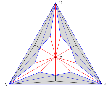
Figure 4.1. This shows 2 generations of repeated stellar subdivision of $T_{1}(y),T_{2}(y)$ and $T_{3}(y)$. The link in $Z$ of the vertex $y$ can be identified with the closure of the shaded region, together with a triangle with vertices $A,B,C$.

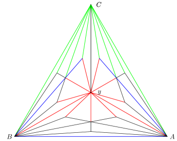
Figure 4.2. This shows 2 generations of repeated stellar subdivision of $T_{1}(y),T_{2}(y)$ and $T_{3}(y)$, the link in $Z$ of the edge between $y$ and $C$ can be identified with the closure of the blue edges.

Lemma 13.

The link of a vertex or edge in $Z$ is contractible. In particular all links of simplices of codimension $>1$ in $Z$ are connected.

Proof.

Let $Y$ be the 1 dimensional subcomplex of Theorem 11. Let $\Delta^{(2)}$ be the $2$-skeleton of a standard $3$-simplex $\Delta.$

Since $Z$ is the clique complex of $Y$ it is possible to characterize links of simplices in $Z$ purely in terms of cliques in $Y.$ Precisely, the link of a simplex $s$ in $Z$ is the collection of all cliques in $Y$ that are disjoint from $s$ but that together with $s$ form a clique.

We view $Y$ as a graph drawn on $|\Delta^{(2)}|$. For every vertex $y$ of $Y$ there are $3$ other vertices $A(y),B(y),C(y)$ of $Y$ such that

1. $y,A,B$ and $C$ are a clique in $Y$.

2. Every vertex adjacent to $y$ in $Y$ is contained in one of the triangles $T_{1}(y)$,$T_{2}(y)$ or $T_{3}(y)$ in $|\Delta^{(2)}|$ with vertices $(A,B,y)$, $(B,C,y)$ or $(A,C,y)$ respectively. In the case $y$ is a vertex of $\Delta$, these triangles are faces of $|\Delta|.$ Otherwise they are all contained in the same face of $|\Delta|$ that contains $y$.

3. More precisely, every vertex of $Y$ adjacent to $y$, and all edges between these vertices, are generated by repeated stellar subdivision of the triangles $T_{1}$,$T_{2}$ and $T_{3}$ together with the edges and vertices of the $T_{i}$.

These observations mean that all links of vertices of $Z$ look the same and can be calculated by drawing the same picture. Similarly all links of edges can be calculated in the same way.

Figure 4.1 shows the link of the central vertex $y$, truncating after 2 iterations of the stellar subdivision. The red edges are incident with $y$. The blue edges are edges not incident with $y$ but whose vertices are adjacent to $y$. Cliques in the link of $y$ in $Z$ are cliques relative to blue edges. We observe that since the drawing of this part of $Y$ is planar, the blue cliques of size 3 other than $\{A,B,C\}$ bound nonoverlapping regions, so we can identify the geometric realization of the link of $y$ in $Z$ with the closure of the shaded triangles here, together with an extra triangle with vertices $A,B,C$. This geometric realization is visibly a topological disc. The effect of iterating stellar subdivision is that the shaded region encroaches inwards, but its homotopy type doesn’t change.

Similarly the link of the edge between $y$ and $C$ is approximated in Figure 4.2. Green edges emanate from $C$ and red emanate from $y$. A blue edge has both vertices adjacent to both $y$ and $C$ (i.e. having incident red and green edges). The closure of the blue edges hence approximates the link of $\{y,C\}$ in $Z$ and is homeomorphic to a line segment. Iterating stellar subdivision extends the segment on both signs and as before, the homotopy type doesn’t change. ∎

Since $Z$ is connected we obtain the following consequence of Lemma 13 (cf. Hatcher [8, pg. 3, proof of Corollary]). The basic idea is to use Lemma 13 to inductively deform any path in $Z$ away from codimension $>1$ simplices.

Corollary 14.

$G$ is connected.

Lemma 15.

G is acyclic.

Proof.

Suppose $G$ has a cycle, so that there is a series of nonrepeating flips that map a vertex $\Delta_{0}=\{\alpha,\beta,\gamma,\delta\}$ to itself. Pick the ordering $\Delta=(\alpha,\beta,\gamma,\delta)$ of this vertex. By Theorem 4 there is a hyperbolic structure $J$ on $\Sigma$ so that $\langle J,\Delta\rangle=(2,2,2,2).$ The flips of $\Delta_{0}$ yield a unique nonrepeating series of flips of $\Delta$ that in turn yield a unique nonrepeating series of Markoff-Hurwitz moves $m_{i}$ preserving $(2,2,2,2)$. By Corollary 6 the series of flips has to be empty. ∎

These results (Corollary 14 and Lemma 15) conclude the proof of Theorem 10 since we established $G$ is an acyclic connected graph that we also know to be 4-valent.

In the rest of this section we prove that smaller pieces of $G$ are connected and acyclic. Specifically, for any simplex $\Delta\in Z$ we may form $G_{\Delta}$, the subgraph of $G$ induced by vertices containing $\Delta$. For example, if $\Delta$ is a 2-simplex then $G_{\Delta}$ has two vertices and an edge representing a flip between them. If $\Delta$ is a 3-simplex then $G_{\Delta}$ has only one vertex, $\Delta$. More generally,

Proposition 16.

For all $\Delta\subset Z$, $G_{\Delta}$ is a tree.

Proof.

Since $G$ is acyclic it suffices to prove $G_{\Delta}$ is connected. We give the proof that $G_{\delta}$ is connected in the case $\delta$ is a vertex of $Z$, the case $\Delta$ is an edge is similar and we have already discussed the other cases.

Suppose $\delta$ is a vertex of $\Delta,\Delta^{\prime}\in Z^{3}$. We aim to connect $\Delta$ to $\Delta^{\prime}$ by flips that don’t touch $\delta$. Order $\Delta$ and $\Delta^{\prime}$ so that $\delta$ is the final element of each. Let $J$ be the hyperbolic structure provided by Theorem 4 such that $\langle J,\Delta\rangle=(2,2,2,2)$. Since $\Delta^{\prime}=(\beta_{1},\beta_{2},\beta_{3},\delta)$, $\langle J,\Delta^{\prime}\rangle=(x_{1},x_{2},x_{3},2)$ for some $x_{1},x_{2},x_{3}\in\mathbb{\mathbf{Z}}.$ The infinite descent (Theorem 5) for $V(\mathbb{\mathbf{Z}}_{+})$ now yields a series of flips that never modifies $\delta$, starts at $\Delta^{\prime}$ and ends at some $\Delta^{\prime\prime}=(\gamma_{1},\gamma_{2},\gamma_{3},\delta)\in Z_{\mathrm{ord}}^{3}$ with $\langle J,\Delta^{\prime\prime}\rangle=(2,2,2,2).$ Also note that by combining Theorem 5 and Theorem 10, there is a unique $\Delta_{0}\in Z^{3}$ such that $\langle J,\Delta_{0}\rangle=(2,2,2,2)$ for any ordering of $\Delta_{0}$. Therefore up to reordering, $\Delta^{\prime\prime}=\Delta_{0}=\Delta$ as required. ∎

There is a nice corollary of Proposition 16 that may be of independent interest.

Corollary 17.

The curve complex $Z$ has the homotopy type of a point.

Proof.

The collection $\{G_{\Delta}:\Delta\>\>\text{$0$-dimensional}\}$ is a cover of $G$ by subcomplexes. The nerve of this cover can be identified with $Z$, and each finite nonempty intersection of the covering complexes is $G_{\Delta}$ for $\Delta$ a simplex of $Z$, and hence is contractible by Proposition 16. Therefore the Nerve Theorem [4, ch. VII, Thm. 4.4] applies to give the result. ∎

5. Proof of theorem 2

Let $\Gamma$ denote the mapping class group of $\Sigma$. Mapping classes in $\Gamma$ may permute the punctures of $\Sigma$. The group $\Gamma$ acts simplicially on $Z$ in the obvious way.

Recall that for each 3-dimensional simplex $\Delta=\{\alpha,\beta,\gamma,\delta\}\in Z$, there is a unique flip of $\alpha$ that produces a new simplex $\{\alpha^{\prime},\beta,\gamma,\delta\}$. Further to this, Huang and Norbury [10] construct a corresponding unique mapping class $\gamma_{\Delta}^{1}\in\Gamma$ that maps $\{\alpha,\beta,\gamma,\delta\}$ to $\{\alpha^{\prime},\beta,\gamma,\delta\}$, similarly $\gamma_{\Delta}^{2}$ performs a flip at $\beta$ and so on.

The mapping class elements $\gamma_{\Delta}^{i}$ can be extended to a cocycle for the group action of $\mathcal{G}$ on $Z_{\mathrm{ord}}^{3}$. In other words, for every $\Delta\in Z_{\mathrm{ord}}^{3}$ and $g\in\mathcal{G}$ there is a mapping class group element $\gamma(g,\Delta)$ such that $\gamma(g,\Delta)\Delta=g\Delta.$ For example, if $g_{1}$ is the generator of the first factor of $\mathcal{G}$ then $\gamma(g,\Delta)=\gamma_{\Delta}^{1}$.

Proposition 18.

For any given $\Delta$, if $\tilde{\Delta}\in Z_{\mathrm{ord}}^{3}$ is an ordering of $\Delta$ then the map

$$\mathcal{G} \to Z^{3}$$

(5.1) $$g \mapsto\gamma(g,\tilde{\Delta}).\Delta$$

is a bijection.

Proof.

The map $g\mapsto\gamma(g,\tilde{\Delta})\Delta$ yields a graph homomorphism from the Cayley graph of $\mathcal{G}$, a 4-regular tree, to $G$. Recall that $G$ is also a 4-regular tree by Theorem 10. The homomorphism is locally injective. Therefore $g\mapsto\gamma(g,\tilde{\Delta})\Delta$ is a bijection. ∎

The next proposition allows us to pass from counting over $G$ to counting over simple closed curves (our goal), up to finite subsets at either side of the passage.

Proposition 19.

Let $J\in\mathcal{T}(\Sigma)$ and for arbitrary fixed $\Delta_{0}\in Z_{\mathrm{ord}}^{3}$ let $o:=\langle J,\Delta_{0}\rangle$. Let $K$ be a compact $S_{4}$-invariant subset of $V(\mathbf{R}_{+})$ containing the set $K(\mathcal{G}.o)$ from Theorem 9. Since $K$ is $S_{4}$-invariant, the condition $\langle J,\Delta\rangle\notin K$ is independent of the ordering of $\Delta\in Z^{3}$, and so well defined. The map

$$\Phi:\{\>\Delta \in Z^{3}\>:\>\langle J,\Delta\rangle\notin K\>\}\to Z^{0},$$

(5.2) $$\Phi:\{\alpha_{1},\alpha_{2},\alpha_{3},\alpha_{4}\} \mapsto\{\alpha_{i}\}\>:\>\ell_{\alpha_{i}}(J)=\max_{1\leq j\leq 4}\ell_{\alpha_{j}}(J)$$

is a well defined injection whose image is all but finitely many elements of $Z^{0}.$

Proof.

That $\Phi$ is well defined is immediate from Theorem 9, Property A.

Suppose $\delta\in Z^{0}$ is the longest curve in each of $\Delta,\Delta^{\prime}$ with respect to $J$, with $\langle J,\Delta\rangle,\langle J,\Delta^{\prime}\rangle\notin K$. By Proposition 16 there is a series of flips taking $\Delta$ to $\Delta^{\prime}$ and never modifying $\delta$. By Property C of Theorem 9, the first flip creates a curve longer than $\delta$ w.r.t. $J$. This continues, since $\mathcal{G}.o-K$ is stable under outgoing moves, and it is therefore impossible to reach $\Delta^{\prime}\neq\Delta$ since $\delta$ is the largest curve of $\Delta^{\prime}$, but not of any intermediate simplex of the sequence that was generated. This establishes injectivity of $\Phi$.

As for the final statement that the image of (5.2) misses only finitely many curves, let $\delta\in Z^{0}$. We aim to find $(\alpha^{\prime},\beta^{\prime},\gamma,\delta)$ for which $\delta$ is the longest curve with respect to $J$. Say that $\delta$ is bad if $\langle J,\Delta\rangle\in K$ for some $\Delta$ containing $\delta$. Otherwise say $\delta$ is good. Since $K$ is compact, and the set of lengths of one sided simple closed curves in $J$ is discrete, there are only finitely many bad $\delta$. We will prove all good $\delta$ are in the image of $\Phi$. For good $\delta$, begin with any $\Delta\in Z_{\mathrm{ord}}^{3}$ such that $\langle J,\Delta\rangle\notin K$ and $\delta$ is last in $\Delta$. If $\delta$ is the longest curve of $\Delta$ with respect to $J$ then we are done. Otherwise let $(x_{1},x_{2},x_{3},x_{4})=\langle J,\Delta\rangle$. Using Property B of Theorem 9, apply moves at the largest entries of $(x_{1},x_{2},x_{3},x_{4})$ (which do not correspond to $\delta$) until $\delta$ becomes the longest curve. The resulting $(y_{1},y_{2},y_{3},y_{4})=\langle J,\Delta^{\prime}\rangle$ cannot be in $K$, so we are done since $\delta=\Phi(\Delta^{\prime}).$ ∎

We have put all the pieces in place to use the methods of Gamburd, Magee and Ronan [6] to prove Theorem 2. We now give an overview of the method of [6] and explain how what we have already proved extends the method to the current setting.

Step 1. (loc. cit.) begins with a compact set $K$ such that for $x\in\mathcal{G}.o-K$, properties A, B, and C hold. Here, we take $K$ to be the set provided by Theorem 9. It is then deduced from A, B, and C that the number of distinct entries of $x\in\mathcal{G}.o-K$ cannot decrease during an outgoing move. There is a further regularization of $K$ in [6, Section 2.4], by adding to $K$ a large ball $B_{\ell^{\infty}}(R)$ if necessary, in order to assume that if for example $x_{1}\leq x_{2}\leq x_{3}\leq x_{4}$ with $(x_{1},x_{2},x_{3},x_{4})\in\mathcal{G}.o-K$ then

$$x_{3}\geq\frac{1}{2}x_{4}^{\frac{1}{3}},$$

$$\frac{3\log(1-2x_{4}^{-\frac{1}{3}})-3\log 2}{\log x_{4}}\geq-\frac{1}{2},$$

and $x_{4}\geq 10.$ These inequalities play a role in technical estimates throughout the proof, in particular, the proof of [6, Lemma 21]. It is possible to increase $K$ to ensure these hold (and the corresponding inequalities for other ordering of the coordinates of $x$) for the same reasons as in (loc. cit.). Also, without loss of generality, $o\in K$.

Step 2. Recall the quantity $n_{J}^{(1)}(L)$ from our main Theorem 2. Fix $\Delta_{0}\in Z_{\mathrm{ord}}^{3}$ and let $o:=\langle J,\Delta_{0}\rangle$. Let $K$ be the enlarged compact set from Step 1.

Putting Propositions 18 and 19 (for the the current $K$) together gives us

$$n_{J}^{(1)}(L) :=\sum_{\alpha\in Z^{0}}\mathbf{1}\{\ell_{\alpha}(J)\leq L\}$$

(Proposition 19) $$=\sum_{\Delta:\>\langle J,\Delta\rangle\notin K}\mathbf{1}\left\{\max\langle J,\tilde{\Delta}\rangle\leq\sqrt{2\sinh\left(\frac{1}{2}L\right)}\right\}+O_{J}(1)$$

(5.3) (Proposition 18) $$=\sum_{g\in\mathcal{G}:\>\mathcal{G}.o\not\notin K}\mathbf{1}\left\{\max g.o\leq\sqrt{2\sinh\left(\frac{1}{2}L\right)}\right\}+O_{J}(1),$$

where for $\Delta\in Z^{3}$ we wrote $\tilde{\Delta}$ for an arbitrary lift of $\Delta$ to $Z_{\mathrm{ord}}^{3}$. Since

$$\sqrt{2\sinh\left(\frac{1}{2}L\right)}=\sqrt{e^{L/2}-e^{-L/2}}=e^{L/4}(1+O(e^{-L}))$$

the required asymptotic formula for (5.3) as $L\to\infty$ will follow from an estimate of the form

(5.4) $$\sum_{g\in\mathcal{G}:\>\mathcal{G}.o\not\notin K}\mathbf{1}\{\max g.o\leq e^{L}\}=c(o)L^{\beta}+o(L^{\beta}).$$

Note as in [6] that the set $\mathcal{G}.o-K$ breaks up into a finite union

$$\mathcal{G}.o-K=\cup_{i=1}^{N}\mathcal{O}_{i}$$

where each $\mathcal{O}_{i}$ is the orbit of a point $o_{i}\in\mathcal{G}.o-K$ under outgoing moves. The points $o_{i}$ are each one move outside of $K$. The fact there are finitely many $o_{i}$ requires the discreteness of $\mathcal{G}.o$ and the compactness of $K$. Each $\mathcal{O}_{i}$ has the form

$$\mathcal{O}_{i}=\{m_{j_{M}}\ldots m_{j_{3}}m_{j_{2}}m_{j_{1}}o_{i}\>:\>M\geq 0,\>j_{i}\neq j_{i+1},j_{1}\neq j_{0}(i)\}$$

where $j_{0}(i)$ is such that $m_{j_{0}(i)}o_{i}\in K$, or in other words, $m_{j_{0}(i)}$ is not outgoing on $o_{i}$. It can be deduced from A, B, C and preceding remarks that each orbit $\mathcal{O}_{i}$ can be identified with a subset $\mathcal{G}_{i}\subset\mathcal{G}$ via a bijection

$$g\in\mathcal{G}_{i}\mapsto g.o\in\mathcal{O}_{i}.$$

Moreover the $\mathcal{G}_{i}$ are disjoint. Therefore

(5.5) $$\sum_{g\in\mathcal{G}:\>\mathcal{G}.o\not\notin K}\mathbf{1}\{\max g.o\leq e^{L}\} = \sum_{i=1}^{N}\sum_{g\in\mathcal{G}_{i}}\mathbf{1}\{\max g.o\leq e^{L}\}$$

$$= \sum_{i=1}^{N}\sum_{x\in\mathcal{O}_{i}}\mathbf{1}\{\max x\leq e^{L}\}.$$

This reduces the count for $n_{J}^{(1)}(L)$ to a count for each of a finite number of orbits under outgoing moves in a region where A, B and C hold.

Step 3. The methods of [6] now take over, with one important thing to point out. A version of Lemma 8 is crucially used during the proof of [6, Lemma 20]. In that instance [6] can make a better bound than we have, but what is really important is the existence of the uniform $\epsilon>0$ in Lemma 8. This establishes a weaker, but qualitatively the same, version of [6, Lemma 20] that plays the same role in the proof. The rest of the arguments of [6] go through without change to establish

Theorem 20 (Gamburd-Magee-Ronan, adapted).

For each $1\leq i\leq N$ there is a constant $c(\mathcal{O}_{i})>0$ such that

$$\sum_{x\in\mathcal{O}_{i}}\mathbf{1}\{\max x\leq e^{L}\}=c(\mathcal{O}_{i})L^{\beta}+o(L^{\beta}).$$

Using Theorem 20 in (5.5) completes the proof of Theorem 2.

Michael Magee,
Department of Mathematical Sciences,
Durham University,
Lower Mountjoy, DH1 3LE Durham,
United Kingdom
michael.r.magee@durham.ac.uk

References

- [1] Arthur Baragar. Asymptotic growth of Markoff-Hurwitz numbers. Compositio Math., 94(1):1–18, 1994.
- [2] Arthur Baragar. Integral solutions of Markoff-Hurwitz equations. J. Number Theory, 49(1):27–44, 1994.
- [3] Arthur Baragar. The exponent for the Markoff-Hurwitz equations. Pacific J. Math., 182(1):1–21, 1998.
- [4] K. S. Brown. Cohomology of groups, volume 87 of Graduate Texts in Mathematics. Springer-Verlag, New York-Berlin, 1982.
- [5] J. W. S. Cassels. An introduction to Diophantine approximation. Cambridge Tracts in Mathematics and Mathematical Physics, No. 45. Cambridge University Press, New York, 1957.
- [6] A. Gamburd, M. Magee, and R. Ronan. An asymptotic formula for integer points on Markoff-Hurwitz surfaces. arXiv:1603.06267v2, Sept. 2017.
- [7] M. Gendulphe. What’s wrong with the growth of simple closed geodesics on nonorientable hyperbolic surfaces. arXiv:1706.08798v1, June. 2017.
- [8] Allen Hatcher. On triangulations of surfaces. Topology Appl., 40(2):189–194, 1991.
- [9] H. Hu, S. Peow Tan, and Y. Zhang. Polynomial automorphisms of preserving the Markoff-Hurwitz polynomial. arXiv://1501.06955, January 2015.
- [10] Yi Huang and Paul Norbury. Simple geodesics and Markoff quads. Geom. Dedicata, 186:113–148, 2017.
- [11] A. Hurwitz. Über eine Aufgabe der unbestimmten Analysis. Archiv. Math. Phys., 3:185–196, 1907. Also: Mathematisch Werke, Vol. 2, Chapt. LXX (1933 and 1962), 410–421.
- [12] A. Markoff. Sur les formes quadratiques binaires indéfinies. Math. Ann., 17(3):379–399, 1880.
- [13] Maryam Mirzakhani. Growth of the number of simple closed geodesics on hyperbolic surfaces. Ann. of Math. (2), 168(1):97–125, 2008.
- [14] G. McShane and I. Rivin. A norm on homology of surfaces and counting simple geodesics. Internat. Math. Res. Notices, (2):61–69 (electronic), 1995.
- [15] R. C. Penner. The decorated Teichmüller space of punctured surfaces. Comm. Math. Phys., 113(2):299–339, 1987.
- [16] Martin Scharlemann. The complex of curves on nonorientable surfaces. J. London Math. Soc. (2), 25(1):171–184, 1982.