Numerical solutions to large-scale differential Lyapunov matrix equations

Abstract

In the present paper, we consider large-scale differential Lyapunov matrix equations having a low rank constant term. We present two new approaches for the numerical resolution of such differential matrix equations. The first approach is based on the integral expression of the exact solution and an approximation method for the computation of the exponential of a matrix times a block of vectors. In the second approach, we first project the initial problem onto a block (or extended block) Krylov subspace and get a low-dimensional differential Lyapunov matrix equation. The latter differential matrix problem is then solved by the Backward Differentiation Formula method (BDF) and the obtained solution is used to build the low rank approximate solution of the original problem. The process being repeated until some prescribed accuracy is achieved. We give some new theoretical results and present some numerical experiments.

1 Introduction

In the present paper, we consider the differential Lyapunov matrix equation (DLE in short) of the form

$$\left\{\begin{array}[]{l}\dot{X}(t)=A(t)\,X(t)+X(t)\,A^{T}(t)+B(t)B(t)^{T};\;(DLE)\\ \;X(t_{0})=X_{0},\;\;t\in[t_{0},\,T_{f}],\end{array}\right.$$ (1)

where the matrix $A(t)\in\mathbb{R}^{n\times n}$ is assumed to be nonsingular and $B(t)\in\mathbb{R}^{n\times s}$ is a full rank matrix, with $s\ll n$. The initial condition $X_{0}$ is assumed to be a symmetric and positive low-rank given matrix.
Differential Lyapunov equations play a fundamental role in many areas such as control, filter design theory, model reduction problems, differential equations and robust control problems [1, 5]. For those applications, the matrix $A$ is generally sparse and very large. For such problems, only a few attempts have been made to solve (1).

Let us first recall the following theoretical result which gives an expression of the exact solution of (1).

Theorem 1.

[1] The unique solution of the general Lyapunov differential equation

$${\dot{X}}(t)=A(t)\,X+X\,A(t)^{T}+M(t);\;\;X(t_{0})=X_{0}$$ (2)

is defined by

$$X(t)=\Phi_{A}(t,t_{0})X_{0}\Phi^{T}_{A}(t,t_{0})+\int_{t_{0}}^{t}\Phi_{A}(t,\tau)M(\tau)\Phi^{T}_{A}(t,\tau)d\tau.$$ (3)

where the transition matrix $\Phi_{A}(t,t_{0})$ is the unique solution to the problem

$${\dot{\Phi}}_{A}(t,t_{0})=A(t)\Phi_{A}(t,t_{0}),\;\;\Phi_{A}(t_{0},t_{0})=I.$$

Futhermore, if $A$ is assumed to be a constant matrix, then we have

$$X(t)=e^{(t-t_{0})A}X_{0}e^{(t-t_{0})A^{T}}+\int_{t_{0}}^{t}e^{(t-\tau)A}M(\tau)e^{(t-\tau)A^{T}}d\tau.$$ (4)

We notice that the problem (1) is equivalent to the linear ordinary differential equation

$$\left\{\begin{array}[]{c c l}\dot{x}(t)&=&\mathcal{A}(t)x(t)+b(t)\\ x_{0}&=&vec(X_{0})\end{array}\right.$$ (5)

where $\mathcal{A}=I\otimes A(t)+A(t)\otimes I$, $x(t)=vec(X(t))$ and $b(t)=vec(B(t)B(t)^{T})$, where $vec(Z)$ is the long vector obtained by stacking the columns of the matrix $Z$. For moderate size problems, it is then possible to use an integration method to solve (5). However, this approach is not adapted to large problems. In the present paper, we will consider projection methods onto extended block Krylov (or block Krylov if $A$ is not invertible) subspaces associated to the pair $(A,B)$. These subspaces are defined as follows

$$\mathbb{K}_{m}(A,B)={\rm range}(B,AB,\ldots,A^{m-1}B)$$

for block Krylov subspaces, or

$${\cal K}_{m}(A,B)={\rm range}(A^{-m},\ldots,A^{-1}B,B,AB,\ldots,A^{m-1}B)$$

for extended block Krylov subspaces. Notice that the extended Krylov subspace ${\cal K}_{k}(A,B)$ is a sum of two block Krylov subspaces

$${\cal K}_{m}(A,B)=\mathbb{K}_{m}(A,B)\,+\,\mathbb{K}_{m}(A^{-1},A^{-1}B).$$

To compute an orthonormal basis $\{V_{1},\ldots,V_{m}\}$, where $V_{i}$ is of dimension $n\times s$ for the block Krylov and $n\times 2s$ in the extended block Krylov case, two algorithms have been defined: the first one is the well known block Arnoldi algorithm and the second one is the extended block Arnoldi algorithm [7, 25]. These algorithms also generate block Hessenberg matrices ${\bar{\cal T}_{m}}={\cal V}_{m+1}^{T}\,A\,{\cal V}_{m}$ satisfying the following algebraic relations

$$A\,{\cal V}_{m} = {\cal V}_{m+1}\,{\bar{\cal T}}_{m},$$ (6)

$$= {\cal V}_{m}\,{\cal T}_{m}+V_{m+1}\,T_{m+1,m}\,E_{m}^{T},$$ (7)

where ${\cal T}_{m}={\bar{\cal T}_{m}}(1:d,:)={\cal V}_{m}^{T}A{\cal V}_{m}$ and where $T_{i,j}$ is the $(i,j)$ block of ${\bar{\cal T}_{m}}$ of size $d\times d$, and $E_{m}=[O_{d\times(m-1)d},I_{d}]^{T}$ is the matrix of the last $d$ columns of the $md\times md$ identity matrix $I_{md}$ with $d=s$ for the block Arnoldi and $d=2s$ for the extended block Arnoldi.
When the matrix $A$ is nonsingular and when the computation of $W=A^{-1}V$ is not difficult (which is the case for sparse and structured matrices), the use of the extended block Arnoldi is to be preferred.
The paper is organized as follows: In Section 2, we present a first approach based on the approximation of the exponential of a matrix times a block using a Krylov projection method. We give some theoretical results such as an upper bound for the norm of the error and an expression of the exact residual. A second approach,presented in Section 3, for which the initial differential Lyapunov matrix equation is projected onto a block (or extended block) Krylov subspace. Then, the obtained low dimensional differential Lyapunov equation is solved by using the well known Backward Differentiation Formula (BDF). In Section 4, an application to balanced truncation method for large scale linear-time varying dynamical systems is presented. The last section is devoted to some numerical experiments.

2 The first approach: using an approximation of the matrix exponential

In this section, we give a new approach for computing approximate solutions to large differential equations (1). The expression of the exact solution as

$$X(t)=e^{(t-t_{0})A}X_{0}e^{(t-t_{0})A^{T}}+\int_{t_{0}}^{t}e^{(t-\tau)A}\,BB^{T}e^{(t-\tau)A^{T}}\,d\tau,$$ (8)

suggests the idea of computing $X(t)$ by approximating the factor $e^{(t-\tau)A}B$ and then using a quadrature method to compute the desired approximate solution.
As computing the exponential of a small matrix is straightforward , this is not the case for large scale problems, as $e^{(t-\tau)A}$ could be dense even though $A$ is sparse. However, in our problem, the computation of $e^{(t-\tau)A}$ is not needed as we will rather consider the product $e^{(t-\tau)A}\,B$, for which approximations via projection methods onto block or extended block Krylov subspaces are well suited.
Krylov subspace projection methods generate a sequence of nested subspaces (Krylov or extended Krylov subspaces). Let $\mathcal{V}_{m}=[V_{1},\ldots,V_{m}]$ be the orthogonal matrix whose columns form an orthonormal basis of the subspace $\mathit{K}_{m}$, Following [21, 22, 27], an approximation to $Z=e^{(t-\tau)A}\,B$ can be obtained as

$$Z_{m}(t)=\mathcal{V}_{m}e^{(t-\tau)\mathcal{T}_{m}}\,\mathcal{V}_{m}^{T}B$$ (9)

where $\mathcal{T}_{m}=\mathcal{V}^{T}_{m}A\mathcal{V}_{m}$. Therefore, the term appearing in the integral expression (8) can be approximated as

$$e^{(t-\tau)A}BB^{T}e^{(t-\tau)A^{T}}\approx Z_{m}(t)Z_{m}(t)^{T}.$$ (10)

If for simplicity, we assume $X_{t_{0}}=0$, an approximation to the solution of the differential Lyapunov equation (8) can be expressed as

$$X_{m}(t)=\mathcal{V}_{m}G_{m}(t){\mathcal{V}_{m}}^{T},$$ (11)

where

$$G_{m}(t)=\displaystyle\int_{t_{0}}^{t}{\widetilde{G}}_{m}(\tau){\widetilde{G}}_{m}^{T}(\tau)d\tau,$$ (12)

and ${\widetilde{G}}_{m}(\tau)=e^{(t-\tau)\mathcal{T}_{m}}B_{m}$.
The next result shows that the matrix function $G_{m}$ is the solution of a low-order differential Lyapunov matrix equation.

Theorem 2.

Let $G_{m}(t)$ be the matrix function defined by (12), then it satisfies the following low-order differential Lyapunov matrix equation

$${\dot{G}}_{m}(t)=\mathcal{T}_{m}G_{m}(t)+G_{m}(t){\mathcal{T}_{m}}^{T}+B_{m}B_{m}^{T},\;t\in[t_{0},\,T_{f}]$$ (13)

Proof.

The proof can be easily derived from the expression (12) and the result of Theorem 1. ∎

As a consequence, intruducing the residual $R_{m}(t)=\displaystyle{\dot{X}}_{m}(t)-A\,X_{m}-X_{m}\,A^{T}-BB^{T}$ associated to the approximation $X_{m}$, we have the following relation

$${\cal V}^{T}_{m}R_{m}(t){\cal V}_{m} = {\cal V}^{T}_{m}({\dot{X}}-AX_{m}(t)-X_{m}(t)A^{T}-BB^{T}){\cal V}_{m}$$

$$= {\dot{G}}_{m}(t)-\mathcal{T}_{m}G_{m}(t)-G_{m}(t){\mathcal{T}_{m}}^{T}-B_{m}B_{m}^{T}$$

$$= 0,$$

which shows that the residual satisfies a Petrov-Galerkin condition.

As mentioned earlier, once ${\widetilde{G}}_{m}(\tau)$ is computed, we use a quadrature method to approximate the integral (12) in order to approximate $G_{m}(t)$.
We now briefly discuss some practical aspects of the computation of $e^{(t-\tau)\mathcal{T}_{m}}B_{m}$ where $B_{m}={\cal V}_{m}^{T}B$, when $m$ is small and $\mathcal{T}_{m}$ is a an upper block Hessenberg matrix.

In the last decade, many approximation techniques such as the use of partial fraction expansions or Padé approximation have been proposed, see for example [9, 22]. However, it was remarked that a good way for evaluating the exponential of matrix times by a vector by using rational approximation to the exponential function. One of the main advantages of rational approximations as compared to polynomial approximations is the better stability of their integration schemes. Let us consider the rational function

$$F(z)=a_{0}+\displaystyle\sum_{i=1}^{p}\frac{a_{i}}{z-\theta_{i}},$$

where the $\theta_{i}$’s are the poles of the rational function $F$. Then, the approximation to ${\widetilde{G}}_{m}(\tau)=e^{(t-\tau)\mathcal{T}_{m}}$ is given by

$${\widetilde{G}}_{m}(\tau)\approx a_{0}B_{m}+\displaystyle\sum_{i=1}^{p}a_{i}[{(t-\tau)\mathcal{T}_{m}}-\theta_{i}I]^{-1}\,B_{m}.$$ (14)

One of the possible choices for the rational function $F$ is based on Chebychev approximation of the function $e^{x}$ on $[0,\,\infty[$, see [22]. We notice that for small values of $m$, one can also directly compute the matrix exponential $e^{(t-\tau){\mathcal{T}}_{m}}$ by using the well-known ’scaling and squaring method for the matrix exponential’ method, [13]. This method was associated to a Padé approximation and is implemented in the expm Matlab routine.

From now on, we assume that the basis formed by the orthonormal columns of ${\cal V}_{m}$ is obtained by applying the block Arnoldi or the extended block Arnoldi algorithm to the pair $(A,B)$.
The computation of $X_{m}(t)$ (and of $R_{m}(t)$) becomes expensive as $m$ increases. So, in order to stop the iterations, one has to test if $\parallel R_{m}\parallel<\epsilon$ without having to compute extra products involving the matrix $A$. The next result shows how to compute the residual norm of $R_{m}(t)$ without forming the approximation $X_{m}(t)$ which is computed in a factored form only when convergence is achieved.

Theorem 3.

Let $X_{m}(t)={\cal V}_{m}G_{m}(t){\cal V}_{m}^{T}$ be the approximation obtained at step $m$ by the block (or extended block) Arnoldi method. Then the residual $R_{m}(t)$ satisfies

$$\parallel R_{m}(t)\parallel=\parallel T_{m+1,m}\bar{G}_{m}(t)\parallel,$$ (15)

where $\bar{G}_{m}$ is the $d\times md$ matrix corresponding to the last $d$ rows of $G_{m}$ where $d=s$ when using the block Arnoldi and $d=2s$ for the extended block Arnoldi.

Proof.

The proof of this theorem comes directly from (11) and the fact that $G_{m}$ solves the low dimensional problem (13). ∎

The result of Theorem 3 is very important in practice, as it allows us to stop the iterations when convergence is achieved without computing the approximate solution $X_{m}(t)$.
The following result shows that the approximation $X_{m}$ is an exact solution of a perturbed differential Lyapunov equation.

Theorem 4.

Let $X_{m}(t)$ be the approximate solution given by (11). Then we have

$${\dot{X}}_{m}(t)=(A-F_{m})\,X_{m}+X_{m}\,(A-F_{m})^{T}+BB^{T}.$$ (16)

where $F_{m}=V_{m}\,T_{m+1,m}^{T}\,V_{m+1}^{T}$.

Proof.

The proof is easily obtained from (13) and the expression (11) of the approximate solution $X_{m}(t)$.
∎

Remark 1.

The solution $X_{m}(t)$ can be given as a product of two low rank matrices. Consider the eigen-decomposition of the symmetric and positive matrix $md\times md$ $G_{m}(t)=U\,D\,U^{T}$ where $D$ is the diagonal matrix of the eigenvalues of $G_{m}(t)$ sorted in decreasing order and $d=s$ for the block Arnoldi or $d=2s$ for the extended block Arnoldi. Let $U_{l}$ be the $md\times l$ matrix of the first $l$ columns of $U$ corresponding to the $l$ eigenvalues of magnitude greater than some tolerance $dtol$. We obtain the truncated eigen-decomposition $G_{m}(t)\approx U_{l}\,D_{l}\,U_{l}^{T}$ where $D_{l}={\rm diag}[\lambda_{1},\ldots,\lambda_{l}]$. Setting ${\widetilde{Z}}_{m}(t)={\cal V}_{m}\,U_{l}\,D_{l}^{1/2}$, it follows that

$$X_{m}(t)\approx{\widetilde{Z}}_{m}(t){\widetilde{Z}}_{m}(t)^{T}.$$ (17)

Therefore, one has to compute and to store only the matrix ${\widetilde{Z}}_{m}(t)$ which is usually the required factor in some control problems such as in the balanced truncation method for model reduction in large scale dynamical systems. This possibility is very important for storage limitations in the large scale problems.

The next result states that the error matrix $X(t)-X_{m}(t)$ satisfies a differential Lyapunov matrix equation.

Theorem 5.

Let $X(t)$ be the exact solution of (1) and let $X_{m}(t)$ be the approximate solution obtained at step $m$. The error $E_{m}(t)=X(t)-X_{m}(t)$ satisfies the following equation

$${\dot{E}}_{m}(t)=AE_{m}(t)+E_{m}(t)A^{T}-R_{m}(t),$$ (18)

and

$$E_{m}(t)=e^{(t-t_{0})A}E_{m,0}e^{(t-t_{0})A^{T}}+\int_{t_{0}}^{t}e^{(t-\tau)A}R_{m}(\tau)e^{(t-\tau)A^{T}}d\tau,\;t\in[t_{0},\,T_{f}].$$ (19)

where $E_{m,0}=E_{m}(0)$.

Proof.

The result is easily obtained by subtracting the residual equation from the initial differential Lyapunov equation (1). ∎

Next, we give an upper bound for the norm of the error in the case where $A$ is a stable matrix.

Theorem 6.

Assume that $A$ is a stable matrix and $X(t_{0})=X_{m}(t_{0})$. Then we have the following upper bound

$$\parallel E_{m}(t)\parallel\leq\displaystyle\parallel T_{m+1,m}\parallel\,\parallel\bar{G}_{m}\parallel_{\infty}\frac{e^{2(t-t_{0})\mu_{2}(A)}-1}{2\mu_{2}(A)},\\$$ (20)

where $\mu_{2}(A)=\displaystyle\frac{1}{2}\lambda_{max}(A+A^{T})<0$ is the 2-logarithmic norm and $\parallel\bar{G}_{m}\parallel_{\infty}=\displaystyle\max_{\tau\in[t_{0},\,t]}\parallel\bar{G}_{m}(\tau)\parallel$. The matrix $\bar{G}_{m}$ is the $d\times md$ matrix corresponding to the last $d$ rows of $G_{m}$ where $d=s$ when using the block Arnoldi and $d=2s$ for the extended block Arnoldi.

Proof.

We first remind that if $A$ is a stable matrix, then the logarithmic norm provides the following bound $\parallel e^{tA}\parallel\leq e^{\mu_{2}(A)t}$. Therefore, using the expression (19), we obtain the following relation

$$\parallel E_{m}(t)\parallel\leq\displaystyle\int_{t_{0}}^{t}\parallel e^{(t-\tau)A}\parallel^{2}\,\parallel R_{m}(\tau)\parallel d\tau.$$

Therefore, using (15) and the fact that $\parallel e^{(t-\tau)A}\parallel\leq e^{(t-\tau)\mu_{2}(A)}$, we get

$$\parallel E_{m}(t)\parallel \leq \parallel T_{m+1,m}\bar{G}_{m}\parallel_{\infty}\displaystyle\int_{t_{0}}^{t}e^{2(t-\tau)\mu_{2}(A)}d\tau$$

$$\leq \parallel T_{m+1,m}\parallel\,\parallel\bar{G}_{m}\parallel_{\infty}e^{2t\mu_{2}(A)}\displaystyle\int_{t_{0}}^{t}e^{-2\tau\mu_{2}(A)}d\tau$$

$$\leq \parallel T_{m+1,m}\parallel\parallel\bar{G}_{m}\parallel_{\infty}e^{2t\mu_{2}(A)}\,\times\frac{e^{-2\mu_{2}(A)t}-e^{-2\mu_{2}(A)t_{0}}}{-2\mu_{2}(A)}$$

$$= \displaystyle\parallel T_{m+1,m}\parallel\,\parallel\bar{G}_{m}\parallel_{\infty}\frac{e^{2(t-t_{0})\mu_{2}(A)}-1}{2\mu_{2}(A)},$$

which gives the desired result.

∎

Notice that if $\parallel T_{m+1,m}\parallel$ is close to zero, which is the case when $m$ is close to the degree of the minimal polynomial of $A$ for $B$, then Theorem 6 shows that the error $E_{m}(t)$ tends to zero.

Next, we give another error bound for the norm of the error for every matrix $A$.

Theorem 7.

Let $X(t)$ be the exact solution to (1) and let $X_{m}(t)$ be the approximate solution obtained at step $m$. Then we have

$$\|X(t)-X_{m}(t)\| \leq \,e^{t\mu_{2}(A)}(\|B\|+\|B_{m}\|)\int_{t_{0}}^{t}e^{-\tau\mu_{2}(A)}\|e^{(t-\tau)A}B-{\cal V}_{m}e^{(t-\tau)\mathcal{T}_{m}}B_{m}\|d\tau$$

where $\mu_{2}(A)=\lambda_{max}((A+A^{T})/2)$, $Z(\tau)=e^{(t-\tau)A}B$ and $Z_{m}(\tau)={\cal V}_{m}e^{(t-\tau)\mathcal{T}_{m}}B_{m}$ with $B_{m}={\cal V}_{m}^{T}B$.

Proof.

From the expressions of $X(t)$ and $X_{m}(t)$, we have

$$\|X(t)-X_{m}(t)\| = \left\|\int_{t_{0}}^{t}(Z(\tau)Z(\tau)^{T}-Z_{m}(\tau)Z_{m}(\tau)^{T})d\tau\right\|$$

$$= \left\|\int_{t_{0}}^{t}[Z(\tau)(Z(\tau)-Z_{m}(\tau))^{T}+(Z(\tau)-Z_{m}(\tau))Z^{T}_{m}(\tau)]d\tau\right\|$$

$$\leq \int_{t_{0}}^{t}(\|Z(\tau)\|+\|Z_{m}(\tau)\|)\|Z(\tau)-Z_{m}(\tau)\|d\tau,$$

Therefore, using the fact that $\mu_{2}(\mathcal{T}_{m})=\lambda_{max}((\mathcal{T}_{m}+\mathcal{T}_{m}^{T})/2)\leq\lambda_{max}((A+A^{T})/2)=\mu_{2}(A)$, where $\mathcal{T}_{m}=\mathcal{V}_{m}^{T}A\mathcal{V}_{m}$, it follows that

$$\|X(t)-X_{m}(t)\| \leq e^{t\mu_{2}(A)}(\|B\|+\|B_{m}\|)\int_{t_{0}}^{t}e^{-\tau\mu_{2}(A)}\|Z(\tau)-Z_{m}(\tau)\|d\tau$$

$$\leq \,e^{t\mu_{2}(A)}(\|B\|+\|B_{m}\|)\int_{t_{0}}^{t}e^{-\tau\mu_{2}(A)}\|e^{(t-\tau)A}B-{\cal V}_{m}e^{(t-\tau)\mathcal{T}_{m}}B_{m}\|d\tau,$$

∎

When using a block Krylov subspace method such as the block Arnoldi method, then one can generalize to the block case the results already stated in many papers; see [7, 9, 12, 22]. In particular, we can easily generalize the result given in [22] for the case $s=1$ to the case $s>1$. In this case, we have the following upper bound.

$$\|e^{A}B-{\cal V}_{m}e^{\mathcal{T}_{m}}B_{m}\|\leq 2\parallel B\parallel\;\displaystyle\frac{\rho^{m}e^{\rho}}{m!},$$ (21)

where $\rho=\|A\|$

The rupper bound (21) could be used in Theorem 7 to obtain a new upper bound for the norm of the error. In that case, we obtain the following upper bound

$$\|X(t)-X_{m}(t)\|\leq 2\parallel B\parallel\displaystyle\frac{\rho^{m}}{m!}\,e^{t(\mu_{2}(A)+\rho)}(\|B\|+\|B_{m}\|)\int_{t_{0}}^{t}e^{-\tau(\mu_{2}(A)+\rho)}(t-\tau)^{m}d\tau,\\$$ (22)

We summarize the steps of our proposed first approach (using the extended block Arnoldi) in the following algorithm

Algorithm 1 The extended block Arnoldi (EBA-exp) method for DLE’s

• Input $X_{0}=X(t_{0})$, a tolerance $tol>0$, an integer $m_{max}$.

• For $m=1,\ldots,m_{max}$

  • Apply the extended block Arnoldi algorithm to compute an orthonormal basis ${\mathcal{V}}_{m}=[V_{1},...,V_{m}]$ of ${\mathcal{K}}_{m}(A,B)=Range[B,A^{-1}B,...,A^{-m}B,A^{m-1}B]$ and the upper block Hessenberg matrix ${\mathcal{T}}_{m}$.

  • Set ${B}_{m}={\mathcal{V}}_{m}^{T}B$ and compute ${\widetilde{G}}_{m}(\tau)=e^{(t-\tau)\mathcal{T}_{m}}B_{m}$ using the matlab function expm.

  • Use a quadrature method to compute the integral (12) and get an approximation of $G_{m}(t)$ for each $t\in[t_{0},\,T_{f}]$.

  • If $\parallel R_{m}(t)\parallel=\parallel T_{m+1,m}\bar{G}_{m}(t)\parallel<tol$ stop and compute the approximate solution $X_{m}(t)$ in the factored form given by the relation (17).

• End

3 A second approach: Projecting and solving with BDF

3.1 Low-rank approximate solutions via BDF

In this section, we show how to obtain low rank approximate solutions to the differential Lyapunov equation (1) by projecting directly the initial problem onto small block Krylov or extended block Krylov subspaces.
We first apply the block Arnoldi algorithm (or the extended block Arnoldi) to the pair $(A,B)$ to get the matrices ${\cal V}_{m}$ and ${\cal T}_{m}={\cal V}^{T}_{m}A{\cal V}_{m}$. Let $X_{m}(t)$ be the desired low rank approximate solution given as

$$X_{m}(t)={\cal V}_{m}Y_{m}(t){\cal V}_{m}^{T},$$ (23)

satisfying the Petrov-Galerkin orthogonality condition

$${\cal V}_{m}^{T}R_{m}(t){\cal V}_{m}=0,\;t\in[t_{0},\;T_{f}],$$ (24)

where $R_{m}(t)$ is the residual $R_{m}(t)=\displaystyle{\dot{X}}_{m}(t)-A\,X_{m}(t)-X_{m}(t)\,A^{T}-BB^{T}$. Then, from (23) and (24), we obtain the low dimensional differential Lyapunov equation

$${\dot{Y}}_{m}(t)-{\cal T}_{m}\,Y_{m}(t)-Y_{m}(t)\,{\cal T}_{m}^{T}-B_{m}B_{m}^{T}=0,$$ (25)

with ${\cal T}_{m}={\cal V}^{T}_{m}A{\cal V}_{m}$ and ${B}_{m}={\cal V}_{m}^{T}\,B$. The obtained low dimensional differential Lyapunov equation (25) is the same as the one given by (13). For this second approach, we have to solve the latter low dimensional differential Lyapunov equation by some integration method such as the well known Backward Differentiation Formula (BDF).
Notice that we can also compute the norm of the residual without computing the approximation $X_{m}(t)$ which is also given, when convergence is achieved, in a factored form as in (17). The norm of the residual is given as

$$\parallel R_{m}(t)\parallel=\parallel T_{m+1,m}\bar{Y}_{m}(t)\parallel,$$ (26)

where $\bar{Y}_{m}$ is the $d\times md$ matrix corresponding to the last $d$ rows of $Y_{m}$ where $d=s$ when using the block Arnoldi and $d=2s$ for the extended block Arnoldi.

3.2 BDF for solving the low order differential Lyapunov equation (25)

In this subsection, we will apply the Backward Differentiation Formula (BDF) method for solving, at each step $m$ of the block (or extended) block Arnoldi process, the low dimensional differential Lyapunov matrix equation (25). We notice that BDF is especially used for the solution of stiff differential equations.
At each time $t_{k}$, let $Y_{m,k}$ of the approximation of $Y_{m}(t_{k})$, where $Y_{m}$ is a solution of (25). Then, the new approximation $Y_{m,k+1}$ of $Y_{m}(t_{k+1})$ obtained at step $k+1$ by BDF is defined by the implicit relation

$$Y_{m,k+1}=\displaystyle\sum_{i=0}^{p-1}\alpha_{i}Y_{m,k-i}+h_{k}\beta{\mathcal{F}}(Y_{m,k+1}),$$ (27)

where $h_{k}=t_{k+1}-t_{k}$ is the step size, $\alpha_{i}$ and $\beta_{i}$ are the coefficients of the BDF method as listed in Table 1 and ${\mathcal{F}}(X)$ is given by

$${\mathcal{F}}(Y)={\cal T}_{m}\,Y+Y\,{\cal T}_{m}^{T}+\,B_{m}\,B_{m}^{T}.$$

$p$	$\beta$	$\alpha_{0}$	$\alpha_{1}$	$\alpha_{2}$
1	1	1
2	2/3	4/3	-1/3
3	6/11	18/11	-9/11	2/11

Table 1: Coefficients of the $p$-step BDF method with $p\leq 3$.

The approximate $Y_{m,k+1}$ solves the following matrix equation

$$-Y_{m,k+1}+h_{k}\beta({\cal T}_{m}Y_{m,k+1}+Y_{m,k+1}{\cal T}_{m}^{T})+BB^{T}+\displaystyle\sum_{i=0}^{p-1}\alpha_{i}Y_{m,k-i}=0,$$

which can be written as the following Lyapunov matrix equation

$$\mathbb{T}_{m}\,Y_{m,k+1}+\,Y_{m,k+1}\mathbb{T}_{m}^{T}+\mathbb{B}_{m,k}\,\mathbb{B}_{m,k}^{T}=0.$$ (28)

We assume that at each time $t_{k}$, the approximation $Y_{m,k}$ is factorized as a low rank product $Y_{m,k}\approx Z_{m,k}{Z_{m,k}}^{T}$, where $Z_{m,k}\in\mathbb{R}^{n\times m_{k}}$, with $m_{k}\ll n$. In that case, the coefficient matrices appearing in (28) are given by

$$\mathbb{T}_{m}=h_{k}\beta{\cal T}_{m}-\displaystyle\frac{1}{2}I\;\mbox{and}\;\mathbb{B}_{m,k+1}=[\sqrt{h_{k}\beta}B^{T},\sqrt{\alpha_{0}}Z_{m,k}^{T},\ldots,\sqrt{\alpha_{p-1}}Z_{m,k+1-p}^{T}]^{T}.$$

The Lyapunov matrix equation (28) can be solved by applying direct methods based on Schur decomposition such as the Bartels-Stewart algorithm [3, 11]. We notice that for large problems, many Krylov subspace type methods have been proposed to solve (28); [8, 14, 15, 16, 17, 25, 21].

Remark 2.

The main difference between Approach 1 and Approach 2 is the fact that in the first case, we compute an approximation of an integral using a quadrature formulae while in the second case, we have to solve a low dimensional differential Lyapunov equation using the BDF method. Mathematically, the two approaches are equivalent and they differ only in the way of computing numerically the low-order approximations: $G_{m}$ in the first approach and $Y_{m}$ in the second one.

‘

We summarize the steps of our proposed first approach (using the extended block Arnoldi) in the following algorithm

Algorithm 2 The extended block Arnoldi (EBA-BDF) method for DLE’s

• Input $X_{0}=X(t_{0})$, a tolerance $tol>0$, an integer $m_{max}$.

• For $m=1,\ldots,m_{max}$

  • Apply the extended block Arnoldi algorithm to compute an orthonormal basis ${\mathcal{V}}_{m}=[V_{1},...,V_{m}]$ of ${\mathcal{K}}_{m}(A,B)=Range[B,A^{-1}B,...,A^{-m}B,A^{m-1}B]$ and the upper block Hessenberg matrix ${\mathcal{T}}_{m}$.

  • Set ${B}_{m}={\mathcal{V}}_{m}^{T}B$ and use the BDF method to solve the low dimensional differential Lyapunov equation

    $${\dot{Y}}_{m}(t)-{\cal T}_{m}\,Y_{m}(t)-Y_{m}(t)\,{\cal T}_{m}^{T}-B_{m}B_{m}^{T}=0,\;t\in[t_{0},\,T_{f}]$$

  • If $\parallel R_{m}(t)\parallel=\parallel T_{m+1,m}\bar{Y}_{m}(t)\parallel<tol$ stop and compute the approximate solution $X_{m}(t)$ in the factored form given by the relation (17).

• End

4 Application: Balanced truncation for linear time-varying dynamical systems

In this section, we assume that the coefficient matrices $A$ and $B$ are time-dependent. It is the case for example when we are dealing with Multi-Input Multi-Output (MIMO) linear-time varying (LTV) dynamical systems

$$\left\{\begin{array}[]{lcl}\dot{x}(t)&=&A(t)x(t)+B(t)u(t),\;x(t_{0})=0,\\ y(t)&=&C(t)x(t),\end{array}\right.$$ (29)

where $x(t)\in\mathbb{R}^{n}$ is the state vector, $u(t)\in\mathbb{R}^{p}$ is the control and $y(t)\in\mathbb{R}^{p}$ is the output. The matrices $A(t)\in\mathbb{R}^{n\times n}$, $B(t)\in\mathbb{R}^{n\times p}$ and $C(t)\in\mathbb{R}^{p\times n}$ are assumed to be continuous and bounded for all $t\in[t_{0},\,T_{f}]$.
The LTV dynamical system (29) can also be denoted as

$${\Sigma}(t)\equiv\left[\begin{array}[]{c|c}A(t)&B(t)\\ \hline\cr C(t)&0\end{array}\right].$$ (30)

In many applications, such as circuit simulation, or time dependent PDE control problems, the dimension $n$ of ${\Sigma}$ is quite large, while the number of inputs and outputs is small $p\ll n$. In these large-scale settings, the system dimension makes the computation infeasible due to memory, time limitations and ill-conditioning. To overcome these drawbacks, one approach consists in reducing the model. The goal is to produce a low order system that has similar response characteristics as the original system with lower storage requirements and evaluation time.
The reduced order dynamical system can be expressed as follows

$${\ \Sigma}_{m}\left\{\begin{array}[]{lll}{\dot{x}}_{m}(t)=A_{m}(t)x_{m}(t)+B_{m}(t)u(t)\\ \\ y_{m}(t)=C_{m}(t)x_{m}(t)\\ \end{array}\right.$$ (31)

where $x_{m}\in\mathbb{R}^{m}$, $y_{m}\in\mathbb{R}^{p}$, $A_{m}\in\mathbb{R}^{m\times m}$, $B\in\mathbb{R}^{m\times p}$ and $C_{m}\in\mathbb{R}^{p\times m}$ with $m\ll n$. The reduced dynamical system (31) is also represented as

$$\Sigma_{m}(t)\equiv\left[\begin{array}[]{c|c}A_{m}(t)&B_{m}(t)\\ \hline\cr C_{m}(t)&0\end{array}\right].$$ (32)

The reduced order dynamical system should be constructed in order that

• The output $y_{m}(t)$ of the reduced system approaches the output $y(t)$ of the original system.

• Some properties of the original system such as passivity and stability are preserved.

• The computation methods are steady and efficient.

One of the well known methods for constructing such reduced-order dynamical systems is the balanced truncation method for LTV systems [23, 24, 26]; see also [10, 19, 20] for the linear time-independent case. This method requires the LTV controllability and observability Gramians $P(t)$ and $Q(t)$ defined as the solutions of the differential Lyapunov matrix equations

$${\dot{P}}(t)=A(t)P(t)+P(t)A(t)^{T}+B(t)B(t)^{T},\;P(t_{0})=0,$$ (33)

and

$${\dot{Q}}(t)=A^{T}(t)P(t)+P(t)A(t)+C(t)^{T}C(t),\;Q(T_{f})=0.$$ (34)

Using the formulae (3), the differential Lyapunov equation (33) has the unique symmetric and positive solution $P(t)$ given by

$$P(t)=\int_{t_{0}}^{t}\Phi_{A}(t,\tau)B(\tau)B^{T}(\tau)\Phi^{T}_{A}(t,\tau)d\tau,$$

where the transition matrix $\Phi_{A}(t,\tau)$ is the unique solution of the problem

$${\dot{\Phi}}_{A}(t,\tau)=A(t)\Phi_{A}(t,\tau),\;\;\Phi_{A}(t,t)=I.$$

The observability Gramian is given by

$$Q(t)=\int_{t}^{T{{}_{f}}}\Phi^{T}_{A}(\tau,t)C^{T}(\tau)C(\tau)\Phi_{A}(\tau,t)d\tau.$$

The two LTV controllability and observability Gramians $P(t)$ and $Q(t)$ are then used to construct a new balanced system such that $\tilde{P}(t)=\tilde{Q}(t)=diag(\sigma_{1}(t),\ldots,\sigma_{n}(t))$ where the Hankel singular values are given by $\sigma_{i}(t)=\sqrt{\lambda_{i}(P(t)Q(t)}$, $i=1,\ldots,n$ and order in decreasing order.
The concept of balancing is to a transform the original LTV system to an equivalent one in which the states that are difficult to reach are also difficult to observe, which is finding an equivalent new LTV system such that the new Gramians ${\widetilde{P}}$ and ${\widetilde{Q}}$ are such that

$${\widetilde{P}}(t)={\widetilde{Q}}(t)=diag(\sigma_{1},\ldots,\sigma_{n})$$

where $\sigma_{i}$ is the $i$-th Hankel singular value of the LTV system; i.e.

$$\sigma_{i}=\sqrt{\lambda_{i}(P(t)Q(t))}.$$

Consider the Cholesky decompositions of the Gramians $P$ and $Q$:

$$P(t)=L_{c}(t)L_{c}(t)^{T},\;\;Q(t)=L_{o}(t)L_{o}(t)^{T},$$ (35)

and consider also the singular value decomposition of $L_{c}(t)^{T}L_{o}(t)$ as

$$L_{c}(t)^{T}L_{o}(t)=Z(t)\Sigma(t)Y(t)^{T},$$ (36)

where $Z(t)$ and $Y(t)$ are unitary $n\times n$ matrices and $\Sigma$ is a diagonal matrix containing the singular values. The balanced truncation consists in determining a reduced order model by truncating the states corresponding to the small Hankel singular values. Under certain conditions stated in [24], one can construct the low order model ${\Sigma}_{m}(t)$ as follows: We set

$$V_{m}(t)=L_{o}(t)Y_{m}(t)\Sigma_{m}(t)^{-1/2}\;{\rm and}\;W_{m}(t)=L_{c}(t)Z_{m}(t)\Sigma_{m}(t)^{-1/2},$$ (37)

where $\Sigma_{m}(t)=diag(\sigma_{1}(t),\ldots,\sigma_{m}(t))$; $Z_{m}(t)$ and $Y_{m}(t)$ correspond to the leading $m$ columns of the matrices $Z(t)$ and $Y(t)$ given by the singular value decomposition (36). The matrices of the reduced LTV system

$$W_{m}(t)^{T}V_{m}(t)A_{m}(t)=V_{m}(t)^{T}A(t)W_{m}(t)-V_{m}(t)^{T}{\dot{W}}_{m}(t),\;B_{m}(t)=V_{m}(t)^{T}B(t),\;C_{m}(t)=C(t)W_{m}(t).$$ (38)

The use of Cholesky factors in the Gramians $P(t)$ and $Q(t)$ is not applicable for large-scale problems. Instead, one can compute low rank approximations of $P(t)$ an $Q(t)$ as given by (17) and use them to construct an approximate balanced truncation model.

As $A$, $B$ and $C$ are time-dependent, the direct application of the two approaches we developed is too expensive. Instead, we can apply directly an integration method such as BDF to the differential Lyapunov matrix equations (33) and (34). Then, at each iteration of the BDF method, we obtain a large Lyapunov matrix equation that can be numerically solved by using the extended block Arnoldi algorithm.
Consider the differential matrix equation (33), then, at each iteration of the BDF method, the approximation $P_{k+1}$ of $P(t_{k+1})$ where $P$ is the exact solution of (33), is given by the implicit relation

$$P_{k+1}=\displaystyle\sum_{i=0}^{p-1}\alpha_{i}P_{k-i}+h_{k}\beta{\mathcal{G}}(G_{k+1}),$$ (39)

where $h_{k}=t_{k+1}-t_{k}$ is the step size, $\alpha_{i}$ and $\beta_{i}$ are the coefficients of the BDF method as listed in Table 1 and ${\mathcal{G}}(X)$ is given by

$${\mathcal{G}}(X)=A^{T}\,X+X\,A+\,B\,B^{T}.$$

The approximate solution $P_{k+1}$ solves the following matrix equation

$$-P_{k+1}+h_{k}\beta(A^{T}P_{k+1}+P_{k+1}A+BB^{T})+\displaystyle\sum_{i=0}^{p-1}\alpha_{i}P_{k-i}=0,$$

which can be written as the following continuous-time algebraic Riccati equation

$$\mathcal{A}_{k}^{T}\,P_{k+1}+\,P_{k+1}\,\mathcal{A}_{k}+\mathcal{B}_{k}\,\mathcal{B}_{k}^{T}=0.$$ (40)

Assuming that at each timestep, $P_{k}$ can be approximated as a product of low rank factors $P_{k}\approx\tilde{Z}_{k}\tilde{Z}_{k}^{T}$, $\tilde{Z}_{k}\in\mathbb{R}^{n\times m_{k}}$, with $m_{k}\ll n$, the coefficient matrices are given by

$$\mathcal{A}_{k}=h_{k}\beta A-\displaystyle\frac{1}{2}I,~{}~{}\mbox{and }\mathcal{B}_{k+1}=[\sqrt{h_{k}\beta}B,\sqrt{\alpha_{0}}\tilde{Z}_{k}^{T},\ldots,\sqrt{\alpha_{p-1}}\tilde{Z}_{k+1-p}^{T}]^{T}.$$

A good way for solving the Lyapunov matrix equation (40) is by using the block or extended block Arnoldi algorithm applied to the pair $(\mathcal{A}_{k},\mathcal{B}_{k})$. This allows us to obtain low rank approximate solutions in factored forms. The procedure is as follows: applying for example the block Arnoldi to the pair $(\mathcal{A}_{k},\mathcal{B}_{k})$ we get, at step $m$ of the Arnoldi process, an orthonormal basis of the extended block Krylov subspace formed by the columns of the matrices: $\{V_{1,k},\ldots,V_{m,k}\}$ and also a block upper Hessenberg matrix $\mathbb{H}_{m,k}$. Let $\mathbb{V}_{m,k}=[V_{1,k},\ldots,V_{m,k}]$ and $\mathbb{H}_{m,k}=\mathbb{V}_{m,k}^{T}\mathcal{A}_{k}\mathbb{V}_{m,k}$. Then the obtained low rank approximate solution to the solution $P_{k+1}$ of (40) is given as $P_{m,k}=\mathbb{V}_{m,k}\mathbb{Y}_{m,k}\mathbb{V}_{m,k}^{T}$ where $\mathbb{Y}_{m,k}$ is solution of the following low order Lyapunov equation

$$\mathbb{H}_{m,k}\mathbb{Y}_{m,k}+\mathbb{Y}_{m,k}{\mathbb{H}_{m,k}}^{T}+{\mathcal{\tilde{B}}}_{k}\,{{\mathcal{\tilde{B}}}_{k}}^{T}=0,$$ (41)

where $\mathcal{\tilde{B}}_{k}=\mathbb{V}_{m,k}^{T}\,\mathcal{B}_{k}$. As stated in Remark 1, the approximate solution can be given in a factored form.

5 Numerical examples

In this section, we compare the two approaches presented in this paper. The exponential approach (EBA-exp) summarized in Algorithm 1, which is based on the approximation of the solution to (1) applying a quadrature method to compute the projected exponential form solution (12). We used a scaling and squaring strategy, implemented in the MATLAB expm function; see [12, 18] for more details. The second method (Algorithm 2) is based on the BDF integration method applied to the projected Lyapunov equation (25). The basis of the projection subspaces were generated by the extended block Arnoldi algorithm for both methods. All the experiments were performed on a laptop with an Intel Core i7 processor and 8GB of RAM. The algorithms were coded in Matlab R2014b.

Example 1. The matrix $A$ was obtained from the 5-point discretization of the operators

$$L_{A}=\Delta u-f_{1}(x,y)\frac{\partial u}{\partial x}+f_{2}(x,y)\frac{\partial u}{\partial y}+g_{1}(x,y),$$

on the unit square $[0,1]\times[0,1]$ with homogeneous Dirichlet boundary conditions. The number of inner grid points in each direction is $n_{0}=$ and the dimension of the matrix $A$ was $n=n_{0}^{2}=$. Here we set $f_{1}(x,y)=10xy$, $f_{2}(x,y)=e^{x^{2}y}$, $f_{3}(x,y)=100y$, $f_{4}(x,y)={x^{2}y}$ , $g_{1}(x,y)=20y$ and $g_{2}(x,y)=x\,y$. The time interval considered was $[0,\,2]$ and the initial condition $X_{0}=X(0)$ was choosen as the low rank product $X_{0}=Z_{0}Z_{0}^{T}$, where $Z_{0}=0_{n\times 2}$. For both methods, we used projections onto the Extended Block Krylov subspaces

$${\mathcal{K}}_{k}(A,B)={\rm Range}(B,A\,B,\ldots,A^{m-1}\,B,A^{-1}\,B,\ldots,(A^{-1})^{m}\,B)$$

and the tolerance was set to $10^{-10}$ for the stop test on the residual. For the EBA-BDF method, we used a 2-step BDF scheme with a constant timestep $h$. The entries of the matrix $B$ were random values uniformly distributed on the interval $[0,\,1]$ and the number of the columns in $B$ was $s=2$.
literature. In order to check if our approaches produce reliable results, we began comparing our results to the one given by Matlab’s ode23s solver which is designed for stiff differential equations. This was done by vectorizing our DLE, stacking the columns of $X$ one on top of each other. This method, based on Rosenbrock integration scheme, is not suited to large-scale problems. Due to the memory limitation of our computer when running the ode23s routine, we chose a size of $100\times 100$ for the matrix $A$.

In Figure 1, we compared the component $X_{11}$ of the solution obtained by the methods tested in this section, to the solution provided by the ode23s method from Matlab, on the time interval $[0,\,2]$, for $size(A)=100\times 100$ and a constant timestep $h=10^{-3}$.

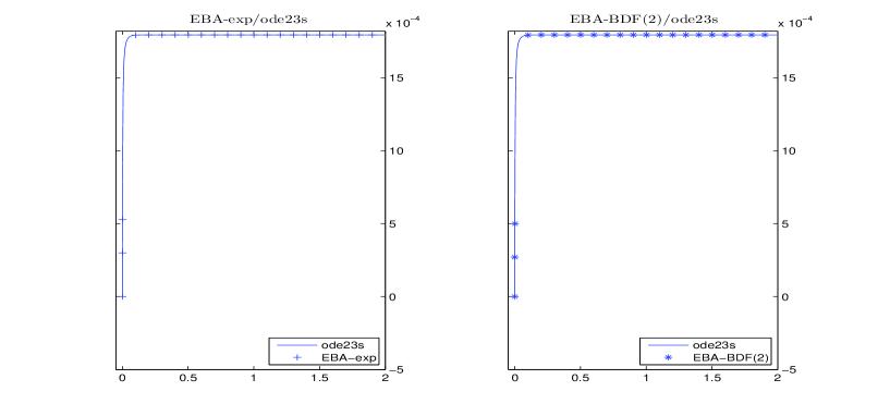
Fig. 1: Values of $X_{11}(t)$ for $t\in[0,\,2]$

We observe that all the considered methods give similar results in terms of accuracy. The relative error norms $\displaystyle{\frac{\|X_{EBA-exp}(t_{f})-X_{ode23s}(t_{f})\|}{\|X_{ode23s(t_{f})}\|}}$ and $\displaystyle{\frac{\|X_{EBA-BDF(2)}(t_{f})-X_{ode23s}(t_{f})\|}{\|X_{ode23s(t_{f})}\|}}$ at final time $t_{f}=2$ were equal to $1.8\times 10^{-10}$ and $9.1\times 10^{-11}$ respectively. The runtimes were respectively 0.59s, 5.1s for the EBA-exp and EBA-BDF(2) methods and 1001s for the ode23s routine.

In Table 2, we give the obtained runtimes in seconds, for the resolution of Equation (1) for $t\in[0,\,2]$, with a timestep $h=0.001$ and the Frobenius norm of the residual at the final time.

size($A$)	EBA-exp	EBA-BDF(2)	Residual norm
$2500\times 2500$	$3.23$ s	$31.9$ s	$\mathcal{O}(10^{-9})$ $(m=16)$
$6400\times 6400$	$5.2$ s	$81.6$ s	$\mathcal{O}(10^{-9})$ $(m=19)$
$10000\times 10000$	$5.6$ s	$168$ s	$\mathcal{O}(10^{-8})$ $(m=19)$
$22500\times 22500$	$11.8$ s	$1546$ s	$\mathcal{O}(10^{-8})$ $(m=23)$

Table 2: runtimes and residual norms for EBA-exp and EBA+BDF(2)

The results in Table 2 illustrate that the EBA-exp method clearly outperforms the EBA-BDF(2) method in terms of computation time even though both methods are equally accurate. In Figure 2, we featured the norm of the residual at final time $t=2$ for both EBA-exp and EBA-BDF(2) methods for size($A$)$=6400\times 6400$ in function of the number $m$ of extended Arnoldi iterations. We observe that the plots coincide for both methods.

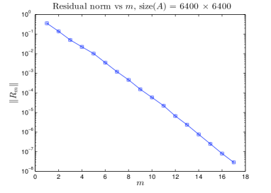
Fig. 2: Residual norms vs the number of extended Arnoldi iterations $m$

Example 2. This example comes from the autonomous linear-quadratic optimal control problem of one dimensional heat flow

$$\frac{\partial}{\partial t}x(t,\eta) = \frac{\partial^{2}}{\partial\eta^{2}}x(t,\eta)+b(\eta)u(t)$$

$$x(t,0) = x(t,1)=0,t>0$$

$$x(0,\eta) = x_{0}(\eta),\eta\in[0,1]$$

$$y(x) = \int_{0}^{1}c(\eta)x(t,\eta)d\eta,x>0.$$

Using a standard finite element approach based on the first order B-splines, we obtain the following ordinary differential equation

$$M\dot{\tt x}(t) = K{\tt x}(t)+Fu(t)$$ (42)

$$y(t) = C{\tt x}(t),$$ (43)

where the matrices $M$ and $K$ are given by:

$$M=\frac{1}{6n}\left(\begin{array}[]{ccccc}4&1&&&\\ 1&4&1&&\\ &\ddots&\ddots&\ddots\\ &&1&4&1\\ &&&1&4\end{array}\right),\;\;K=-\alpha\,n\,\left(\begin{array}[]{ccccc}2&-1&&&\\ -1&2&-1&&\\ &\ddots&\ddots&\ddots\\ &&-1&2&-1\\ &&&-1&2\end{array}\right).$$

Using the semi-implicit Euler method, we get the following discrete dynamical system

$$(M-\Delta tK)\,\dot{x}(t)=M\,x(t)+\Delta t\,Fu_{k}.$$

We set $A=(M-\Delta tK)^{-1}\,M$ and $B=\Delta t\,(M-\Delta tK)^{-1}\,F$. The entries of the $n\times s$ matrix $F$ and the $s\times n$ matrix $C$ were random values uniformly distributed on $[0,\,1]$. In our experiments we used $n=$, $s=2$, $\Delta t=0.01$ and $\alpha=0.05$.

In Table 3, we give the obtained runtimes in seconds, for the resolution of Equation (1) for $t\in[0,\,2]$, with a timestep $h=0.001$ and the Frobenius norm of the residual at the final time.

size($A$)	EBA-exp	EBA-BDF(2)	Residual norms
$2500\times 2500$	$1.0$ s	$8.0$ s	$\mathcal{O}(10^{-11})$ $(m=11)$
$6400\times 6400$	$4.9$ s	$14.4$ s	$\mathcal{O}(10^{-14})$ $(m=11)$
$10000\times 10000$	$11.5$ s	$29.7$ s	$\mathcal{O}(10^{-13})$ $(m=11)$
$20000\times 20000$	$11.8$ s	$173.4$ s	$\mathcal{O}(10^{-13})$ $(m=11)$

Table 3: runtimes and residual norms for EBA-exp and EBA-BDF(2)

The figures in Table 3 illustrate the gain of speed provided by the EBA-exp method. Again, both methods performed similarly in terms of accuracy. In figure 3, we considered the case size($A$)$=100\times 100$ and plotted the upper bound of the error norms as stated in Formula (20) at the final time $T_{f}$ against the computed norm of the errors, taking the solution given by the integral formula (8) as a reference, in function of the number $m$ of Arnoldi iterations for the EBA-exp method.

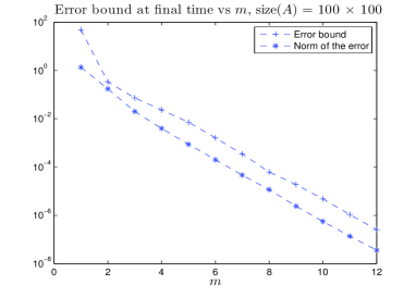
Fig. 3: Upper bounds of the error norms and computed error norms vs the number of iterations

Example 3 In this last example, we applied the EBA-BDF(1) method to the well-known problem Optimal Cooling of Steel Profiles. The matrices were extracted from the IMTEK collection . We compared the EBA-BDF(2) method to the EBA-exp method for problem sizes $n=1357$ and $n=5177$, on the time interval $[0\,,1000]$. The initial value $X_{0}$ was chosen as $X_{0}=0$ and the timestep was set to $h=0.01$. The tolerance for the Arnoldi stop test was set to $10^{-7}$ for both methods and the projected low dimensional Lyapunov equations were numerically solved by the solver (lyap from Matlab) at each iteration of the extended block Arnoldi algorithm for the EBA-BDF(2) method.

size($A$)	EBA-exp	EBA-BDF(2)	Residual norms
$1357\times 1357$	$11.1$ s	$515.5$ s	$\mathcal{O}(10^{-8})$ $(m=6)$
$5177\times 5177$	$148.7$ s	$1721$ s	$\mathcal{O}(10^{-7})$ $(m=39)$

Table 4: Optimal Cooling of Steel Profiles: runtimes and residual norms for EBA-exp and EBA-BDF(2)

In Table 4, we listed the obtained runtimes which again showed the advantage of the EBA-exp method in terms of execution time and similar accuracy for both methods.

6 Conclusion

We presented in the present paper two new approaches for computing approximate solutions to large scale differential Lyapunov matrix equations. The first one comes naturally from the exponential expression of the exact solution and the use of approximation techniques of the exponential of a matrix times a block of vectors. The second approach is obtained by first projecting the initial problem onto a block Krylov (or extended Krylov) subspace, obtain a low dimensional differential Lyapunov equation which is solved by using the well known BDF integration method. We gave some theoretical results such as the exact expression of the residual norm and also upper bounds for the norm of the errors. An application in model reduction for linear time-varying dynamical systems is also given. Numerical experiments show that both methods are promising for large-scale problems, with a clear advantage for the EBA-exp method in terms of computation time.

References

- [1] H. Abou-Kandil, G. Freiling, V. Ionescu, G. Jank, Matrix Riccati Equations in Control and Sytems Theory, in Systems & Control Foundations & Applications, Birkhauser, (2003).
- [2] B.D.O. Anderson, J.B. Moore, Linear Optimal Control, Prentice-Hall, Englewood Cliffs, NJ, (1971).
- [3] R.H. Bartels, G.W. Stewart, Algorithm 432: Solution of the matrix equation AX+XB=C, Circ. Syst. Signal Proc., 13 (1972), 820–826.
- [4] C. Brezinski, Computational Aspects of Linear Control, Kluwer, Dordrecht, 2002.
- [5] M. J. Corless and A. E. Frazho, Linear systems and control - An operator perspective, Pure and Applied Mathematics. Marcel Dekker, New York-Basel, 2003.
- [6] B.N. Datta, Numerical Methods for Linear Control Systems Design and Analysis, Elsevier Academic Press, (2003).
- [7] V. Druskin, L. Knizhnerman, Extended Krylov subspaces: approximation of the matrix square root and related functions, SIAM J. Matrix Anal. Appl., 19(3)(1998), 755–771.
- [8] A. El Guennouni, K. Jbilou and A.J. Riquet, Block Krylov subspace methods for solving large Sylvester equations, Numer. Alg., 29 (2002), 75–96.
- [9] E. Gallopoulos and Y. Saad, Efficient solution of parabolic equations by Krylov approximation methods, SIAM J. Sci. Statist. Comput., 13 (1992), 1236–1264.
- [10] K. Glover, All optimal Hankel-norm approximations of linear multivariable systems and their L-infinity error bounds. International Journal of Control, 39(1984) 1115–1193.
- [11] G.H. Golub, S. Nash and C. Van Loan, A Hessenberg Schur method for the problem , IEEE Trans. Automat. Contr., 24 (1979), 909–913.
- [12] N. J. Higham, The scaling and squaring method for the matrix exponential revisited. SIAM J. Matrix Anal. Appl., 26(4) (2005), 1179-1193.
- [13] N. J. Higham and A. H Al-Mohy, A new scaling and squaring algorithm for the matrix exponential. SIAM J. Matrix Anal. Appl., 31(3) (2009), 970–989.
- [14] D.Y. Hu, L. Reichel, Krylov-subspace methods for the Sylvester equation, Lin. Alg. Appl., 172 (1992), 283–313.
- [15] I.M. Jaimoukha and E.M. Kasenally, Krylov subspace methods for solving large Lyapunov equations, SIAM J. Numer. Anal., 31 (1994), 227–251.
- [16] K. Jbilou, Low-rank approximate solution to large Sylvester matrix equations, App. Math. Comput., 177 (2006), 365–376.
- [17] K. Jbilou and A. J. Riquet, Projection methods for large Lyapunov matrix equations, Lin. Alg. Appl., 415 (2006), 344–358.
- [18] C.B. Moler, C.F. Van Loan, Nineteen Dubious Ways to Compute the Exponential of a Matrix, SIAM Review 20, 1978, pp. 801–836. Reprinted and updated as ”Nineteen Dubious Ways to Compute the Exponential of a Matrix, Twenty-Five Years Later,” SIAM Review 45(2003), 3–49.
- [19] B.C. Moore, Principal component analysis in linear systems: controllability, observability and model reduction, IEEE Trans. Automatic Contr., AC-26(1981), 17–32.
- [20] C. T. Mullis and R. A. Roberts, Synthesis of minimum roundoff noise fixed point digital filters, IEEE Trans. Acoust. Speec Signal Process, 24, 1976.
- [21] Y. Saad, Numerical solution of large Lyapunov equations, in Signal Processing, Scattering, Operator Theory and Numerical Methods. Proceedings of the international symposium MTNS-89, vol. 3, M.A. Kaashoek, J.H. van Schuppen and A.C. Ran, eds., Boston, 1990, Birkhauser, pp. 503–511.
- [22] Y. Saad, Analysis of some Krylov subspace approximations to the matrix exponential operator, SIAM J. Numer. Anal., 29 (1992), 209–228.
- [23] H. Sandberg, Linear Time-Varying Systems: Modeling and Reduction, Ph.D. thesis, Department of Automatic Control, Lund Institute of Technology, Lund, 2002.
- [24] S. Shokoohi, L. Silverman, and P. Van Dooren, Linear time-variable systems: balancing and model reduction, IEEE Trans. Automat. Control, 28 (1983), 810–822.
- [25] V. Simoncini, A new iterative method for solving large-scale Lyapunov matrix equations, SIAM J. Sci. Comp., 29(3) (2007), 1268–1288.
- [26] E. I. Verriest and T. Kailath, On generalized balanced realizations, IEEE Trans. Automat. Control, 28 (1983), 833–844.
- [27] H. van der Vorst, Iterative Krylov Methods for Large Linear Systems, Cambridge University Press, Cambridge, 2003.