Shared Memory Parallel Subgraph Enumeration

Abstract

The subgraph enumeration problem asks us to find all subgraphs of a target graph that are isomorphic to a given pattern graph. Determining whether even one such isomorphic subgraph exists is $\mathcal{NP}$-complete—and therefore finding all such subgraphs (if they exist) is a time-consuming task. Subgraph enumeration has applications in many fields, including biochemistry and social networks, and interestingly the fastest algorithms for solving the problem for biochemical inputs are sequential. Since they depend on depth-first tree traversal, an efficient parallelization is far from trivial. Nevertheless, since important applications produce data sets with increasing difficulty, parallelism seems beneficial.

We thus present here a shared-memory parallelization of the state-of-the-art subgraph enumeration algorithms RI and RI-DS (a variant of RI for dense graphs) by Bonnici et al. [BMC Bioinformatics, 2013]. Our strategy uses work stealing and our implementation demonstrates a significant speedup on real-world biochemical data—despite a highly irregular data access pattern. We also improve RI-DS by pruning the search space better; this further improves the empirical running times compared to the already highly tuned RI-DS.

Keywords: subgraph enumeration; subgraph isomorphism; parallel combinatorial search; graph mining; network analysis

1 Introduction

Graphs are used in a plethora of fields to model relations or interactions between entities. One frequently occurring (sub)task in graph-based analysis is the subgraph isomorphism problem (SGI). It requires finding a smaller pattern graph $G_{p}$ in a larger target graph $G_{t}$ or, equivalently, finding an injection from the nodes of $G_{p}$ to the nodes of $G_{t}$ such that the edges of $G_{p}$ are preserved. The SGI decision problem is $\mathcal{NP}$-complete [1]. Finding all isomorphic subgraphs of $G_{p}$ in $G_{t}$ is commonly referred to as the subgraph enumeration (SGE) problem; this is the problem we deal with in this paper. Note that SGE algorithms require exponential time in the worst case, as there may be exponentially many matches to enumerate.

Efficient algorithms for SGI exist only for special cases such as planar graphs [2], where a linear time algorithm exists for constant query graph size; this method can further be used to count the number of occurrences of the query graph in linear time. Consequently, the most successful tools in practice for more general graphs are quite time-consuming when one or all exact subgraphs are sought [3]. At the same time, the data volumes in common SGI and SGE applications are steadily increasing. Example fields are life science [4], complex network analysis [3, 5], decompilation of computer programs [6], and computer vision [7]. A problem related to SGE is motif discovery, where the goal is to find all frequent subgraphs up to a very small size [8]; note that in our problem, queries consist of only one subgraph. Similar to motif search, works dealing with massive target graphs often focus on very small pattern graphs [9], often with only up to 10-20 vertices. In contrast, we enumerate pattern graphs with several dozens of vertices and hundreds of edges.

In bioinformatics and related life science fields, graphs are used among other things for analyzing protein-protein interaction networks and finding chemical similarities [10]. Such data is often labeled, which further speeds up SGE algorithms by excluding from search those vertex pairs with different labels. The fastest algorithms for SGE on these graphs use a backtracking approach based on depth-first search (DFS) of the search space [11], where often pruning rules are employed to reduce the search space. The fastest such algorithm is RI by Bonnici et al. [4], as evidenced by a recent study by Carletti et al. [12]. RI, as well as other state-of-the-art algorithms, are not parallel and thus there is potential for solving large and/or hard instances faster by parallelization. Distributed SGE algorithms exist (e.g., for MapReduce [3]). However, when the target graph fits into main memory (which is typically the case for the mentioned life science applications), a shared-memory parallelization is much more promising. Parallelizing DFS-based backtracking efficiently is not trivial though [13]. As in our case, this usually stems from a highly irregular data access pattern, which makes load balancing difficult (in particular when enumerating all isomorphic subgraphs).

Contribution

Our contribution is twofold. First, we present a shared memory parallelization of subgraph enumeration algorithms RI and RI-DS (the version of RI for dense graphs) using work stealing with private double-ended queues (see Section 3). We conduct a detailed experimental analysis on three data collections, consisting of fifty target graphs and thousands of pattern graphs from the original RI paper [12]. On these three data collections we achieve parallel speedups of 5.96, 5.21, and 9.49 with 16 workers on long running instances, respectively (see Section 5). The maximum speedup for any single instance is 13.40. Moreover, on one data collection we manage to reduce the number of instances not solved within the time limit of 180 seconds by more than 50%. Second, we introduce an improved version of RI-DS that makes better use of available data by further constraining the search space with minimal overhead (Section 4). It decreases search space size and variability considerably and somewhat reduces the average running time on the three data collections. Our combined improvements give considerable performance gains over state-of-the-art implementations for longer running instances: we achieve speedups of 7.75 (RI), 4.37 (RI-DS) and 13.67 (RI-DS), respectively, over the original implementations on the three data collections used in our experiments.

2 Preliminaries

2.1 Definitions and Notation

Basics

A graph $G=(V,E)$ consists of a set of $n$ vertices $V$ and a set of $m$ edges $E\subseteq V\times V$. Unless stated otherwise, we assume all graphs to be directed. We refer to the set of nodes that have an edge starting or ending at $v$ by $N(v)\subseteq V$ or by neighborhood of $v$. For directed graphs one can also distinguish between incoming and outgoing neighbors. In an undirected graph the degree of a node is the number of edges incident to that node. For the directed case we define the indegree of a node $v$ as $\deg^{-}(v)=|\{u\mid(u,v)\in E\}|$ and the outdegree as $\deg^{+}(v)=|\{w\mid(v,w)\in E\}|$.

Labels

Graphs can be annotated with semantic information by adding labels to nodes or edges. Let $L_{V}$ and $L_{E}$ be the sets of possible node and edge labels, respectively. We define the node label function $lab:V\rightarrow L_{V}$ that associates each node with a label. Similarly, we define the edge label function $\beta:E\rightarrow L_{E}$. We say two nodes $u,v$ are equivalent and write $u\equiv v$ if $lab(u)=lab(v)$. Two edges $e,f$ are compatible if $\beta(e)=\beta(f)$. We assume strict equality for labels but there may be other application-specific equivalence functions.

(Sub)Graph isomorphism

Two graphs $G_{1}=(V_{1},E_{1})$ and $G_{2}=(V_{2},E_{2})$ are considered isomorphic, denoted by $G_{1}\cong G_{2}$, if there is a bijective function $f$ mapping all nodes of $G_{1}$ to nodes of $G_{2}$ such that the edges of the graph are preserved and compatible, and nodes in $G_{1}$ are mapped onto equivalent nodes in $G_{2}$. More formally, $G_{1}\cong G_{2}$ if and only if a bijection $f:V_{1}\rightarrow V_{2}$ exists that fulfills the following properties.

$$\forall u,v\in V_{1}:(u,v)\in E_{1}\iff(f(u),f(v))\in E_{2}$$ (1)

$$\forall v\in V_{1}:v\equiv f(v)$$ (2)

$$\forall(u,v)\in E_{1}:(u,v)\equiv(f(u),f(v))$$ (3)

In subgraph enumeration we must list all (in our case non-induced) subgraphs in a target graph $G_{t}$ that are isomorphic to a pattern graph $G_{p}$. Clearly, subgraph enumeration is not easier than subgraph isomorphism. In practice one can even expect a significant slowdown, even when working in parallel. After all, we cannot stop after a potentially early first hit, but have to explore the search space exhaustively.

2.2 Related Work

2.2.1 Overview

According to Carletti et al. [14], most SGI and SGE algorithms can be categorized as follows.

State space based

A common way to model the SGI/SGE search space is to use a state space representation (SSR) [12], modeling the search space as a tree. Finding a subgraph isomorphism can then be viewed as the problem of finding a mapping $M:V_{p}\rightarrow V_{t}$ that maps nodes of the pattern graph onto nodes of the target graph. If the mapping is injective and does not violate the isomorphism constraints (1) to (3), it yields a subgraph $G_{s}\subseteq G_{t}$ isomorphic to $G_{p}$.

Every node in the tree represents a state of the (partial) mapping; the root represents the empty mapping. A branch taken represents extending the partial mapping by a certain pair of nodes. To find a subgraph isomorphism, one thus needs to find a path in the state space tree of length $|V(G_{p})|$ beginning at the root, such that the equivalent mapping does not violate the graph isomorphism constraints. The key to doing that efficiently is ignoring parts of the state space tree early which cannot be extended to a valid solution. This is especially critical when enumerating all isomorphic subgraphs, since otherwise states at depth $|V(G_{p})|$ in the state space tree would need to be visited. Typically, state space based approaches use depth first search (DFS) in order to search the state space tree and make use of pruning rules in order to remove parts of the search space that do not contain valid solutions [15, 11]. In an independent experimental comparison, Carletti et al. [12] concluded that “RI seems to be currently the best algorithm for subgraph isomorphism” for sparse biochemical graphs. Other popular algorithms of this category besides RI [4] are VF2 [15] and VF2 Plus [14] (VF2 was also part of Carletti et al.’s comparison).

One important distinction between the different state space exploration approaches is the order in which the nodes of the pattern graph are processed. Algorithms like VF2 use a dynamic variable ordering: they decide at every state, based on the nodes already mapped onto the target graph, which node of the pattern graph to examine next. This allows them a greater freedom in eliminating unfruitful branches of the search space but comes with the additional cost of running whatever logic is used to pick the next pattern graph node in every step of the search process. Algorithms like RI and VF2 Plus use a static ordering fixed before the search. This reduces the amount of work done during the search process but means that at any step the selection of the next variable may not be optimal regarding search space size [16]. Since we base our parallelization on RI, a more detailed explanation of the sequential algorithm is worthwhile. As already mentioned, RI uses state space exploration with a search strategy that is static and depends only on the pattern graph. The general idea is to order the nodes of the pattern graph in a way that ensures the next node visited is always the one being most constrained by already matched nodes, while introducing additional constraints as early as possible. During the search no expensive pruning or inference rules are used, trading faster comparisons for a larger search space. The pattern graph nodes are ordered by starting with highly connected nodes and then greedily adding nodes that are connected with already selected nodes. For the actual search process, a set of increasingly expensive rules are checked for each candidate extension.

There is also a version of RI called RI-DS [4] that computes an initial list of possible target nodes for all nodes in $G_{p}$ and is better on medium to large dense graphs [4, 12]. RI and RI-DS participated in the ICPR2014 contest on graph matching algorithms for pattern search in biological databases, “outperforming all other methods in terms of running time and memory consumption” [17].

Index based

Index-based approaches employ an indexing data structure to store features (such as distance in the graph) that can then queried to quickly find a valid extension of a partial mapping. This reduces the time to find an isomorphic subgraph if one exists (called the matching time). Index-based approaches spend more time up front preprocessing the target graph, and are therefore typically used for larger target graphs and very small pattern graphs. Examples include QuickSI [18], GraphQL [19], GADDI [11] and STwig [9].

Constraint propagation based

Modeling the subgraph isomorphism problem as a constraint satisfaction problem (CSP) means that each variable/node in $G_{p}$ has a domain (a set of candidate nodes in $G_{t}$) and a set of constraints that ensure edge preservation and injectivity. Tools in this category focus on reducing the search space at the cost of spending more time to achieve that reduction. The search space reduction is dependent on both the pattern and target graph [4]. LAD [20] is a CSP approach in which initial domains can be based solely on node degrees, but can also incorporate label compatibility. In addition to the constraints above, LAD uses a constraint which results in the removal of values from the domain if using them would imply remaining nodes cannot all be mapped to different nodes. Also, LAD propagates constraints after each assignment to further reduce domains of remaining variables. These groups are not disjoint; LAD for example uses a state space representation with depth first search, but it reduces the search space by using constraint propagation [12].

2.2.2 Parallelism

Parallel backtracking has been considered in recent years both in a generic manner (e.g., [21]) and for specific combinatorial search problems such as maximal clique enumeration [13]. To the best of our knowledge, there are no parallel versions of the newer state-of-the-art algorithms for subgraph enumeration or isomorphism like RI and VF2 Plus. Some work has been done in order to accelerate the search process using GPUs, with an algorithm named GPUSI, but here the focus is on tiny pattern graphs [22]. The work by Shahrivari and Jalili [23] is also for shared memory, but targets motif search. Thus, there are a few critical differences: (i) they search for all subgraphs of a certain size $k$, (ii) this size $k$ is tiny, and (iii) their parallelization approach is simpler due to the problem structure. There is also a CSP based parallel approach for SGI that beats VF2 and LAD on some graphs, but it was not compared to RI nor RI-DS [24]. Of the backtracking approaches there is one parallelization of VF2 [25] using Cilk++. Its authors note that the amount of state copied to enable work stealing results in a lot of overhead. To remedy this, our parallelization copies partial solutions only for stolen tasks, not those that remain private.

RI’s static node ordering, and focus on speed of exploration, makes it a good candidate for parallelization. The static order and lack of complex state should allow for reasonable overhead when distributing work among workers.

3 Parallelizing RI

Perhaps the biggest challenge for fine-grained parallelism is to keep workers from starving. For subgraph isomorphism and enumeration, starvation is even more of a concern, as the search space is highly irregular [26, 27]—few long overlapping search paths exist that lead to solutions. However, there is another challenge: assuming we can find enough tasks for all workers, we need to efficiently communicate tasks, which include a potentially large mapping $M$. We address both of these challenges by combining the work stealing strategy of Acar et al. [28] and task coalescing.

3.1 Task Representation

The search phase of RI iteratively expands a mapping $M$ of nodes from $G_{p}$ onto nodes from $G_{t}$ by choosing vertices according to a static ordering $\mu=[\mu_{1},\ldots,\mu_{V(G_{P})}]$ of the pattern nodes. A natural way to represent a task then would be as a tuple $(M,\mu_{i},v_{t})$ with the current partial mapping $M$, and a check to perform: can we map pattern node $\mu_{i}$ to target node $v_{t}$? If the new mapping is consistent, then the task spawns new tasks $(M^{\prime},\mu_{i+1},v_{c})$ to check if the next pattern node $\mu_{i+1}$ maps to each remaining candidate target node $v_{c}$. While this seems like the ideal representation, it has serious drawbacks. First, the mapping $M$ is potentially large, as it must include every mapped node of $G_{p}$. Second, when executing a task, a worker explores only one state in the search space. Thus, this task representation comes with large overhead: copying $M$ for each new task is too time consuming. For that reason, we design our tasks with several built-in optimizations. First, we do not explicitly store a partial mapping with a task, we instead communicate partial mappings as needed. Therefore, we effectively represent a task by the node pair $(\mu_{i},v_{t})$. Second, when expanding a mapping $M$ to include pattern node $\mu_{i}$ and target node $v_{t}$, we first check the consistency of each new task before spawning it. This reduces the risk of a worker stealing a dead-end task.

3.2 Work stealing with private deques

Our solution is to use the work stealing strategy of Acar et al. [28], which gives each worker $i$ a private double-ended queue (deque) $q_{i}$. Worker $i$ adds and removes from the front of its private deque $q_{i}$, and workers request to steal from the back of other workers’ deques. The private deque serves two purposes for our problem: (i) Tasks at the front of worker $i$’s deque are added and removed in depth-first search order, and therefore worker $i$ always has a correct partial mapping $M_{i}$. Thus, for private tasks, a partial mapping is never copied. (ii) Tasks at the back of a worker’s deque are closer to the root of the search space tree than those near the front. Therefore, when stealing, a worker receives a task with larger part of the tree below them than nodes closer to the leaves. Thus, we expect stolen tasks to be relatively long-running, reducing the number of steals overall. An example of workers stealing and executing tasks can be seen in Fig. 1.

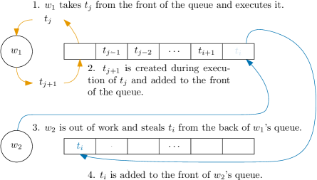
Figure 1: Workers $w_{1}$ and $w_{2}$ and their deques. $w_{1}$ is executing a task and $w_{2}$ is stealing from $w_{1}$.

We quickly point out that an alternative solution would be to use lock-free data structures, which ensure efficient access to tasks for all workers with low overhead [29, 30, 31]. However, they have two drawbacks: first they are notoriously difficult to implement [28], and second, they still require copying a partial map with every task.

Load balancing could either be sender or receiver initiated and is performed by all workers explicitly calling communication methods in their work loops. We implement a receiver-initiated private deque work stealing since its performance is comparable to classic work stealing. Aside from a private deque for each worker, this method requires three shared data structures:

1. work_available—an array of Boolean values, one for each worker, indicating if that worker currently has tasks in its queue.

2. requests—an array of worker ids, used by workers to request a task from another worker.

3. transfers—an array of tasks, used to transfer tasks between workers.

⬇

while not terminated:

if q.is_empty():

acquire_task(worker)

task = q.pop()

work_available[worker] = not q.is_empty()

process_task_requests(worker)

execute(task)

Figure 2: The work loop for work stealing with private deques.

The main loop of a worker consists of taking a task from the deque, updating the entry in work_available. It then checks for a work request in requests, answering that via transfers from the back of its queue if possible and concludes by executing the task it took at the start of the loop. Once it runs out of tasks, it repeatedly requests work from a random worker until it receives a task or is terminated. The main loop can be seen in Fig. 2. Function process_task_requests transfers partial mappings between workers. This design keeps tasks small and reduces overhead when creating tasks. Except for the requests, all data structures are completely unsynchronized.

3.3 Initial work distribution

We initially create tasks corresponding to states directly below the root of the search space tree. Each task maps the node $\mu_{1}$ of the node ordering onto one node of the target graph. At the beginning of the search process, each worker creates an equal number of those tasks and places them in its private deque.

3.4 Task coalescing

One further reason to use work stealing with private deques, is the ease with which we can perform task coalescing [28]—that is, grouping together tasks into task groups that can each be processed as a single unit of work. In general, grouping together tasks that have short execution time can reduce the number of steals—and the number of times we must copy a worker’s partial mapping. This design makes it easy to experiment with the size of task groups to strike a balance between overhead and granularity.

3.5 Termination detection

Finally, we implement a termination detection algorithm, since there is no central scheduler, and we do not know the number of tasks in advance. To detect when all workers terminate, we implement a variant of Dijkstra’s popular termination algorithm [32] described by Schnitger [33]: workers are arranged in a ring and when a worker becomes idle, it passes a token to the next worker. Initially the token is colored white; if a worker is busy, it colors the token black. If the token makes it around the ring and is still white, then all workers terminate. The algorithm has termination delay proportional to the number of workers. As we use no more than 16 workers for our shared memory implementation, this simple approach is sufficient. More efficient algorithms exist for systems with many more workers or more complex topologies [34].

4 Speeding up RI-DS

RI-DS is a variation of RI that is faster on dense graphs [4] and differs from RI by precomputing sets of compatible nodes for each pattern node. These sets are incorporated into the initial node ordering and consistency checks. Before computing the node ordering, RI-DS first computes for each pattern node $v_{p}$ a set of compatible target nodes $D(v_{p})\subseteq G_{t}$ called the domain of $v_{p}$. This process is called domain assignment.

4.1 Domains in RI-DS

Initially, the domain of $v_{p}$, denoted by $D(v_{p})$, is set to all pattern nodes with compatible degrees and equivalent labels. That is, all nodes with in- and outdegree at least that of $v_{p}$’s, and with labels that match $v_{p}$’s.

We then remove each $v_{t}$ from $D(v_{p})$ whose neighborhood is not consistent with the neighborhood of $v_{p}$. For example, let $v_{t}\in D(V_{p})$ and suppose we have an edge $(v_{p},w_{p})\in E(G_{p})$; then we want at least one $w_{t}\in D(w_{p})$ such that $(v_{p},w_{p})\cong(v_{t},w_{t})\in E(G_{t})$. If no such edge exists, then mapping $v_{p}$ onto $v_{t}$ cannot lead to a solution and we can remove $v_{t}$ from $D(v_{p})$. If any domain becomes empty, then there are no isomorphic subgraphs to enumerate. This step is based on arc-consistency (AC) from constraint programming [17, 20].

Domains are used in both the preprocessing and search phases. First, when computing the node ordering $\mu$, all pattern nodes with domain size one (called singleton domains) are placed at the beginning of the ordering. Further, when initializing the search, RI-DS uses domains as candidates for the root node of the search space (unlike RI, which considers $V(G_{t})$). Lastly, during the search, to determine if we can map $\mu_{i}\in V(G_{p})$ onto $v_{t}\in V(G_{t})$, we first check if $v_{t}\in D(\mu_{i})$.

4.2 RI-DS with improved tie-breaking and forward checking

We integrate two improvements into the preprocessing phase of RI-DS: we use domain size to break ties in the node ordering $\mu$, and we further reduce domain sizes with forward checking.

4.2.1 Node ordering

Bonnici and Giugno [17] provide an extensive comparison of node ordering strategies. They show that, while other domain-based orderings occasionally reduce the search space further than RI-DS, RI-DS consistently outperforms other methods. Our goal is to strengthen the node ordering of RI-DS by further using domains, without introducing unacceptable overhead. RI’s node ordering (on which RI-DS is based) is constructed by greedily selecting pattern nodes according to the number of neighbors in the partial ordering (denoted by $w_{m}$), the number of nodes in the ordering reachable via nodes not in the ordering (denoted $w_{n}$), and the degree. We propose to further break ties when two nodes have the same degree, in favor of the node with the smaller domain. That is, when deciding how to order two nodes with identical values $w_{m}$ and $w_{n}$ and identical degrees, we select the one with the smaller domain to appear first in the node ordering. This is a continuation of the constraint-first principle: by preferring the node with the smaller domain, we pick the node which is most constrained first.

4.2.2 Forward checking

In forward checking, a concept in constraint programming, once we assign a value to a variable (in our case, mapping a pattern node onto a target node), we place additional restrictions on the remaining unassigned variables. After assigning a variable, we can remove from the domains of all unassigned variables those values that will violate a constraint because of this assignment [20].

In RI-DS, assignments take place only during the search phase—not while computing domains. Yet, we observe that pattern nodes with singleton domains can only be assigned to a single target node. We therefore perform forward checking for all pattern nodes with singleton domains, as each pattern node will be assigned to its target node in the future.

The constraint we verify is injectivity. For each pattern node with a singleton domain, we remove the target node in that domain from the domains of all other pattern nodes. We repeat this procedure for any newly introduced singleton domains. In RI, domains are implemented as bitmasks, which we use to quickly remove singleton domains’ contents from all other domains.

5 Experimental Evaluation

We now give an in-depth experimental evaluation of our SGE algorithms. Our experimental evaluation is split into two parts. In the first one we evaluate the effectiveness of our parallelization. We do so by comparing our parallel RI against our sequential RI implementation and against the original RI implementation (RI version 3.6). In the second part we compare RI-DS (version 3.51) against our new variants with domain size ordering (RI-DS-SI) and with domain size ordering and forward checking (RI-DS-SI-FC).

Table 1: Graph data collections.

Collection	$|V(G_{T})|$	$|E(G_{T})|$	degree
	$\min/\max$	$\min/\max$	$\mu$	$\sigma$
PPIS32	5 720/12 575	51 464/332 458	27.38	60.88
GRAEMLIN32	1 081/6 726	12 960/230 467	55.41	88.74
PDBSv1	240/33 067	480/61 546	3.06	2.67

5.1 Data collections

We select a subset of the six biochemical data collections tested by Bonnici et al. [4] for the original experiments with RI. We focus on data collections with large graphs that contain hard, long-running instances, as we do not expect easy instances to benefit from parallelism. We select three data collections: PDBSv1, on which RI is more efficient than RI-DS, and PPIS32 and GRAEMLIN32 on which RI-DS is more efficient. Properties of these data collections are listed in Table 1 and described next.

PPI

The PPI data collection consists of large, dense protein-protein interaction networks, which have either 32, 64, 28, 256, 512, 1 024, 2 048, or unique labels; For each label count there is a version with a uniform and one with a normal (Gaussian) distribution. We run our experiments on the variant with 32 normally distributed labels (which we call PPIS32) since it contains the highest number of unsolved instances. PPIS32 has ten target graphs; there are also 420 pattern graphs with 4, 8, 16, 32, 64, 128, and 256 edges, which are are classified as either being dense, semi-dense, or sparse [4].

PDBSv1

The PDBSv1 data collection consists of large, sparse graphs with data from RNA, DNA, and proteins. The 30 target graphs have between 240 and 330 067 nodes. There are 1 760 pattern graphs have 4, 8, 16, 32, 64 or 128 edges. Note that RI could not solve about half of the 128-edge pattern graphs in the 3-minute time limit of the original experiments [4].

Graemlin

The Graemlin data collection consists of medium sized and large graphs from microbial networks. The ten target graphs have between 1 081 and 6 726 vertices. There are 420 pattern graphs with 4, 8, 16, 32, 64, 128, and 256 edges that are grouped into dense, semi-dense and sparse groups. There are different versions of this data collection. One is labeled with unique labels, while the others are labeled with 32, 64, 128, 256, 512, 1 024 and 2 048 different labels using a uniform distribution. The low label versions especially have a high percentage of unsolved instances and longer running times [4]. We use the 32-label version since it is hard and still contains many solvable instances. We refer to it as GRAEMLIN32.

5.2 Experimental platform and results

We run our experiments on a dedicated machine with 256 GB RAM and 2$\times$8 Intel® Xeon® E52680 cores, running openSUSE 13.1 with Linux version 3.12.6252 (x86_64). Our code was compiled using GCC 4.8.1 (gcc-4_8-branch revision 202388) and optimization flag -O3. We use TCMALLOC for memory allocation and pthread for threading.

In the detailed comparison of the algorithms below, we are chiefly concerned with the matching time of the algorithms—the time it takes to enumerate all isomorphic subgraphs. To measure the efficiency of our parallel implementation, we report the speedup of our algorithm as we increase the number of workers. One challenge to measuring the speedup is that the data collections contain many more short running instances than long running instances. Since our goal is to solve long running instances quickly, we must prevent short running instances (which have little speedup) from dominating our measurements. First, we compute the speedup as an arithmetic mean over the total runtime to process all instances of a particular data collection (avg in our tables). We report the standard error of the mean with red bars in our point plots. We further compute the geometric mean (gmean in our tables) of the speedup of each instance. Moreover, we split instances into short and long running groups either by the time required in the original RI/RI-DS implementation or against a single worker of our parallel implementation, depending on the comparison.

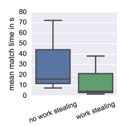
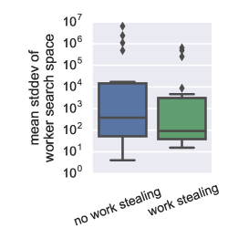
Figure 3: The effects of work stealing with 16 workers on a random sample of instances from PPIS32.

5.2.1 Work stealing

We show the effect of work stealing on our parallelization by measuring the matching time for a sample of PPI with and without work stealing. In Fig. 3, we see that work stealing reduces the time required to find a solution for 16 workers by a factor of 1.65. Without work stealing, the number of states explored by all workers has a high standard deviation, indicating that work is unevenly distributed.

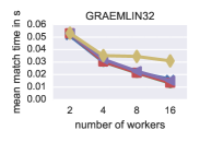
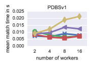
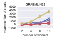
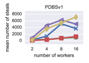
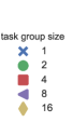
Figure 4: Effects of task group size on match time and number of steals.

5.2.2 Task coalescing

To measure the effect of task coalescing, we vary the task group size. We experiment on a sample of short running instances of PPIS32, PDBSv1 and GRAEMLIN32 using 2, 4, 8, and 16 workers. We repeat each run 15 times to reduce variability and experiment with task group sizes of 1, 2, 4, 8 and 16 tasks. Results with a single worker are not included, as larger task group sizes obviously reduce overhead in that case.

In Fig. 4 we can see that for PDBSv1 a task group size of four is ideal. For GRAEMLIN32 task group sizes of two and four yield the best running time for four or more workers. We note that PPIS32 (not shown here) has similar running times for all task group sizes, except that size 16 is much worse. Furthermore, the two rightmost plots in Fig. 4 clearly show that less work stealing takes place for a task group size of two or four. Notice that large task group sizes (16 for GRAEMLIN32 and 8-16 for PDBSv1) have many more steals than smaller task group sizes. This behavior is due to the irregular search space: few states (and few tasks) have much work below them in the state space tree. For large task group sizes, these tasks end up in single task groups, which are stolen by a single worker. If multiple such task groups are held by a single worker, then other workers can only steal small tasks, which finish quickly and lead to more steals. For our remaining experiments, we use task group size four.

5.2.3 Performance of parallel RI

We measure the performance of parallel RI on PDBSv1 with 1, 2, 4, 8 and 16 workers. Like Bonnici et al. [4] we do not include RI-DS in the comparison on PDBSv1 because it was designed for dense graphs. Likewise we do not test parallel RI on the dense GRAEMLIN32 and PPIS32 sets but rather the versions designed for dense graphs: parallel RI-DS and our improvements.

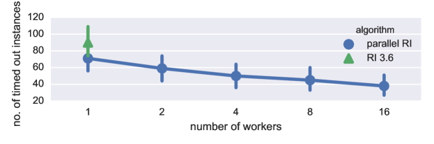
Figure 5: Number of timed out instances on PDBSv1 for RI 3.6 and parallel RI.

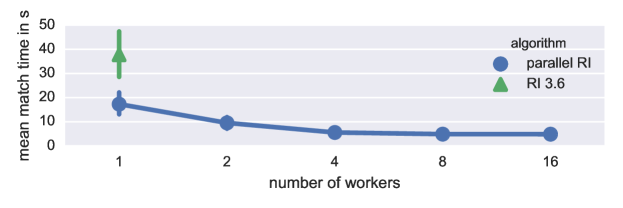
Figure 6: Match time on PDBSv1 for parallel RI on instances with a match time of more than one second.

Table 2: Speedup of parallel RI over our implementation with one worker, for all, short, and long instances. Maximum speedups marked with a $*$ exceeded the worker count, due to a lack of precision when timing short running instances.

# workers	all instances			short ($<1$ sec.)			long ($\geq 1$ sec.)
	avg	gmean	$\max$	avg	gmean	$\max$	avg	gmean	$\max$
2	1.78	1.20	3.37∗	1.71	1.17	3.37∗	1.78	1.75	1.91
4	3.03	1.31	5.20∗	2.30	1.25	5.20∗	3.03	2.88	3.53
8	4.28	0.80	5.92	2.12	0.73	5.47	4.29	3.97	5.92
16	5.90	0.64	10.02	1.84	0.57	5.23	5.96	5.12	10.02

As can be seen in Fig. 5, multithreading significantly reduces the number of unsolved instances for long running instances. While RI 3.6 fails to solve 90 instances in the time limit, parallel RI leaves only 38 instances unsolved with 16 workers. Surprisingly, RI 3.6 is slower than parallel RI with a single worker, which we believe is due to subtle implementation differences. Since it is faster, we therefore compare our parallel RI implementation to itself with one worker. However, before this comparison, we briefly mention how parallel RI compares to RI 3.6. On instances solved by RI 3.6 within the time limit, parallel RI with 16 threads beats RI 3.6 by an average factor of 3.07 on short running instances with 4 workers, and a speedup of 7.75 with 16 workers on long running instances.

Of the 1 760 query graphs in the PDBSv1 data collection, only 160 have a match time of longer than one second with our single threaded implementation. Since short instances do not benefit much from parallelism (as can be seen in Table 2), on average, using more than four workers increases match time. This is not surprising, as easily solved instances have a smaller search space than hard ones, offering little opportunity for improved performance with parallelism. This behavior mirrors the slowdown observed by Acar et al. [28]—where private deque based work stealing reduced search space parallelism. However, for long running instances, increasing the number of workers always improves the speedup. As seen in Table 2, parallel RI reaches an average speedup of 5.96 when running with 16 workers–and even achieves a maximum speedup of 10.01 on some long running instances. This is further corroborated in Fig. 6, where we see that the average match time decreases as we increase the number of workers. The number of unsolved instances decreases similarly, as seen in Fig. 5. We do, however, note that the number of unsolved instances does not decrease linearly with the number of workers.

5.2.4 RI-DS-SI and RI-DS-SI-FC with domain size ordering and forward checking

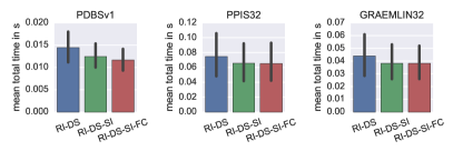
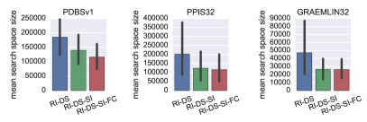
Figure 7: Search space reduction over, and single threaded run time comparison with, RI-DS.

We measure the search space size and total time on PDBSv1, PPIS32 and GRAEMLIN32 with and without our improvements (see Section 4.2) on short running instances with a time limit of one second and on a sample of longer running instances of PPIS32 and GRAEMLIN32.

Search space size

In Fig. 7 we give the search space size and total time for domain size ordering (RI-DS-SI) and for domain size ordering with forward checking (RI-DS-SI-FC). Domain size ordering clearly reduces search space size and total time for all data collections. However, forward checking is less clear. On PDBSv1, forward checking clearly reduces search space size as well as total time. For PPIS32 we see a slight improvement in search space size but no change in time, while for GRAEMLIN32 the search space size remains essentially the same.

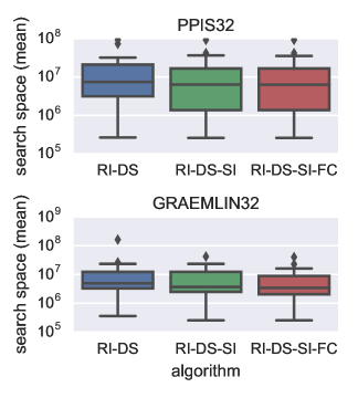
capposition = below, floatrowsep =qquad, [0.5] [0.5]

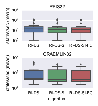
Figure 8: Search space size.

Figure 9: Search speed.

Figure 10: Search space on a random sample of long running instances from GRAEMLIN32 and PPIS32 for our implementation of RI-DS and its variants with one worker. 

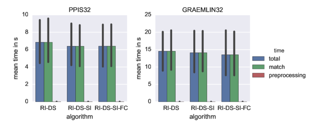
Figure 11: The running time of our implementation of RI-DS and its variants. Note that preprocessing time is negligible.

However, in Fig. 10 we can see that on long running instances of PPIS32, RI-DS-SI clearly reduces the search space size, while RI-DS-SI-FC does not seem to affect search space size at all. Yet, on long running instances of GRAEMLIN32, RI-DS-SI-FC shows a clear improvement over RI-DS-SI. From Fig. 11 we can see that for PPIS32, RI-DS-SI and RI-DS-SI-FC have similar total time and match time and both show improvements in total time over RI-DS. On GRAEMLIN32, RI-DS-SI-FC beats RI-DS-SI and RI-DS in total time, albeit not as strongly as in search space. Mean search space on the GRAEMLIN32 sample is nearly halved from RI-DS to RI-DS-SI-FC, while the mean match time changes from 14.54 ($\sigma=13.3$) to 13.53 ($\sigma=13.86$). This behavior can also be seen in Fig. 10, where the number of explored states per second drops between RI-DS to RI-DS-SI. One possible explanation for these results may be that, while we manage to reduce more search space, we do not change the memory access pattern required for solving an instance. During search, we must iterate over relatively short adjacency lists, implemented as arrays. Skipping a few entries will not lead to large changes in running time, since the running time is dominated by loading the array into memory. Since RI-DS-SI-FC is at least as fast as RI-DS-SI, and further has a smaller search space for the GRAEMLIN32 data collection (shown in Fig. 10(a)), we compare RI-DS-SI-FC with RI-DS in our remaining experiments.

5.2.5 Parallel RI-DS-SI-FC

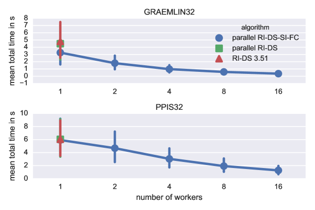
Figure 12: Total time on GRAEMLIN32 and PPIS32 for variants of RI-DS.

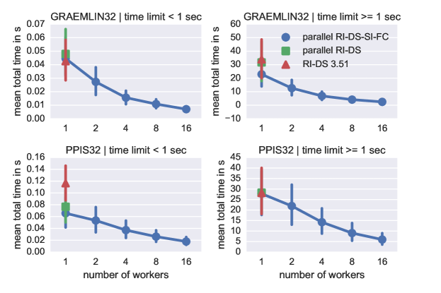
Figure 13: Total time on GRAEMLIN32 and PPIS32 for variants of RI-DS split between instances with a total time of less than one second and longer running instances.

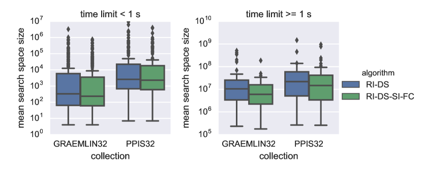
Figure 14: Search space on GRAEMLIN32 and PPIS32 for RI-DS and RI-DS-SI-FC split between short running instances (less than one second) and longer running instances.

We compare parallel RI-DS-SI-FC (our improved version of RI-DS) against our own implementation of RI-DS and the original RI-DS implementation, RI-DS 3.51. We measure the performance on PPIS32 and GRAEMLIN32 with 1, 2, 4, 8 and 16 workers. In Fig. 12 and Fig. 13 we show the total time, including the time for domain assignment and preprocessing. To explain the source of limited scalability, we provide not only the speedups for all instances in Fig. 12; in Fig. 13 we also consider short running instances and long running instances (with less and more than one second total time, respectively) separately.

In Fig. 12 and Fig. 13 we see that our parallelization of RI-DS (parallel RI-DS) with one worker is slightly faster than RI-DS 3.51. For short running instances, RI-DS 3.5.1 is faster on GRAEMLIN32 but slower on PPIS32. However, on long running instances, the trend is reversed; RI-DS 3.51 is slightly faster than parallel RI-DS on GRAEMLIN32 and slower on PPIS32. We conclude that these differences are caused by implementation differences, since the search strategy of parallel RI-DS is the same as that of RI-DS 3.51.

As for the performance of our improved version RI-DS-SI-FC, Fig. 12 shows a reduction in total time of about 38% on GRAEMLIN32 with the mean total time improving from 4.50 seconds ($\sigma=19.25$) to 3.26 seconds ($\sigma=14.16$). Looking at Fig. 13, the improvement is especially pronounced on long running instances. For PPIS32 the situation is reversed. There are some improvements, but in contrast to GRAEMLIN32 on PPIS32 the numbers are improved for the short running instances, not the long running ones. This results in a (small) improvement of about 2% for the overall data collection with RI-DS having a mean total time of 6.04 seconds ($\sigma=20.45$) and RI-DS-SI-FC having a mean total time of 5.93 seconds ($\sigma=20.44$). The reduction in search space size seen in Fig. 14 reflects this as well. The mean search space size for long running PPIS32 instances is small, while for the long running GRAEMLIN32 instances the search space size is reduced to less than a third. Notably, for both data collections, RI-DS-SI-FC reduces variability in search space size. Overall these results reflect the trends in Fig. 11 where speedups for GRAEMLIN32 on long running instances are much stronger than those for PPIS32.

As can be seen in Table 3, speedup is greater on GRAEMLIN32 than PPIS32. The average speedup with 16 threads on long running instances for GRAEMLIN32 is 9.49 while it is 5.21 for PPIS32. Still, both speedups are higher than the mean speedup for parallel RI on PDBSv1 in Table 2. The differences between data collections suggest that inherent parallelism of the instance may be crucial for achieving high speedup. Also, the maximum speedup of 13.40 on GRAEMLIN32 shows that, for some inputs, our implementation is capable of speedups close to the optimum. Interestingly, while the speedup on the denser PPIS32 and GRAEMLIN32 is higher than the speedup on PDBSv1, the number of unsolved instances does not improve as much. The number of unsolved instances in PPIS32 drops from 212 with RI-DS 3.51 to 197 with RI-DS-SI-FC and 16 threads and from 171 to 158 on GRAEMLIN32 respectively—suggesting that GRAEMLIN32 and PPIS32 contain many difficult instances.

Finally, we briefly summarize how our parallel implementation compares to RI-DS 3.51. We achieve the best speedups for instances of GRAEMLIN32 and PPIS32 with 16 threads. For GRAEMLIN32, we achieve speedups of 6.67 on short running instances and 13.67 on long running instances. With PPIS32, we have stronger speedup of 5.12 on short running instances when compared to 4.37 for long running instances.

Table 3: Speedup of parallel RI-DS-SI-FC over itself with one worker, for all, short, and long instances. Maximum speedups marked with a $*$ exceeded the worker count, which we attribute to cache effects for long running instances, and a lack of precision in timing for short running instances.

# workers	all instances			short ($<1$ sec)			long ($\geq 1$ sec)
	avg	gmean	$\max$	avg	gmean	$\max$	avg	gmean	$\max$
GRAEMLIN32
2	1.76	1.57	4.34∗	1.83	1.54	4.34∗	1.76	1.80	2.26∗
4	3.35	2.03	6.26∗	3.25	1.89	6.26∗	3.35	3.28	4.09∗
8	5.55	1.69	9.74∗	4.70	1.43	9.74∗	5.56	5.25	7.13
16	9.45	1.38	13.40	6.92	1.05	12.97	9.49	8.98	13.40
PPIS32
2	1.57	1.63	3.56∗	1.56	1.68	3.56∗	1.57	1.45	2.01∗
4	2.07	2.09	5.66∗	2.25	2.04	5.66∗	2.07	2.25	3.83
8	3.28	1.85	7.78	3.18	1.55	7.78	3.28	3.50	6.74
16	5.20	2.10	13.04	4.80	1.60	11.27	5.21	5.56	13.04

6 Conclusions

In this paper we have presented a shared-memory parallelization for the state-of-the-art subgraph enumeration algorithms RI and RI-DS. Besides a parallelization based on work stealing, we also contribute improved search state pruning using techniques from constraint programming.

On the long running instances of the biochemical data collections we used in our experiments, we achieve notable (although not perfect) speedups, considering the highly irregular data access. We conclude that parallelization often yields a significant acceleration of state space representation based subgraph isomorphism/enumeration algorithms, individual results depend on the input being considered. Future work should thus address a dynamic strategy for determining the optimal level of parallelism during the search process.

References

- [1] R. C. Read and D. G. Corneil, “The graph isomorphism disease,” J. Graph Theor., vol. 1, no. 4, pp. 339–363, 1977.
- [2] D. Eppstein, “Subgraph isomorphism in planar graphs and related problems,” J. of Graph Algorithms and Applications, vol. 3, no. 3, pp. 1–27, 1999.
- [3] L. Lai, L. Qin, X. Lin, and L. Chang, “Scalable subgraph enumeration in MapReduce,” Proc. VLDB Endow., vol. 8, no. 10, pp. 974–985, 2015.
- [4] V. Bonnici, R. Giugno, A. Pulvirenti, D. Shasha, and A. Ferro, “A subgraph isomorphism algorithm and its application to biochemical data.” BMC Bioinformatics, vol. 14, no. Suppl 7, p. S13, 2013.
- [5] K. Erciyes, Complex Networks: An Algorithmic Perspective, 1st ed. Boca Raton, FL, USA: CRC Press, Inc., 2014.
- [6] Y. Liu, Y. Zhao, L. Zhang, and K. Liu, “Subgraph isomorphism based intrinsic function reduction in decompilation,” J. Software Eng. Appl., vol. 9, no. 03, pp. 80–90, 2016.
- [7] P. Le Bodic, P. Héroux, S. Adam, and Y. Lecourtier, “An integer linear program for substitution-tolerant subgraph isomorphism and its use for symbol spotting in technical drawings,” Pattern Recognition, vol. 45, no. 12, pp. 4214–4224, 2012.
- [8] J. A. Grochow and M. Kellis, “Network motif discovery using subgraph enumeration and symmetry-breaking,” Research in Computational Molecular Biology, pp. 92–106, 2007.
- [9] Z. Sun, H. Wang, H. Wang, B. Shao, and J. Li, “Efficient subgraph matching on billion node graphs,” Proc. VLDB Endow., vol. 5, no. 9, pp. 788–799, May 2012.
- [10] N. Dahm, H. Bunke, T. Caelli, and Y. Gao, “Efficient subgraph matching using topological node feature constraints,” Pattern Recognition, vol. 48, no. 2, pp. 317–330, 2014.
- [11] J. Lee, W.-S. Han, R. Kasperovics, and J.-H. Lee, “An in-depth comparison of subgraph isomorphism algorithms in graph databases,” Proc. VLDB Endow., vol. 6, no. 2, pp. 133–144, 2012.
- [12] V. Carletti, P. Foggia, and M. Vento, “Performance comparison of five exact graph matching algorithms on biological databases,” in Proc. 17th Intl. Conf. on Image Analysis and Processing (ICIAP 2013), ser. LNCS, vol. 8158. Springer, 2013, pp. 409–417.
- [13] M. C. Schmidt, N. F. Samatova, K. Thomas, and B.-H. Park, “A scalable, parallel algorithm for maximal clique enumeration,” J. Parallel Distrib. Comput., vol. 69, no. 4, pp. 417–428, 2009.
- [14] V. Carletti, P. Foggia, and M. Vento, “VF2 Plus: An improved version of VF2 for biological graphs,” in Proc. 10th Intl. Workshop on Graph-Based Representations in Pattern Recognition, ser. LNCS, vol. 9069. Springer, 2015, pp. 168–177.
- [15] L. P. Cordella, P. Foggia, C. Sansone, and M. Vento, “A (sub)graph isomoprhism algorithm for matching large graphs,” IEEE Transactions on Pattern Analysis and Machine Intelligence, vol. 26, no. 10, pp. 1367–1372, 2004.
- [16] I. Almasri, X. Gao, and N. Fedoroff, “Quick mining of isomorphic exact large patterns from large graphs,” in IEEE Intl. Conf. on Data Mining Workshop, 2014, pp. 517–524.
- [17] V. Bonnici and R. Giugno, “On the variable ordering in subgraph isomorphism algorithms,” IEEE/ACM Trans. Comput. Biol. Bioinformatics, vol. 14, no. 1, pp. 193–203, 2017.
- [18] H. Shang, Y. Zhang, X. Lin, and J. X. Yu, “Taming verification hardness: an efficient algorithm for testing subgraph isomorphism,” Proc. VLDB Endow., vol. 1, no. 1, pp. 364–375, 2008.
- [19] H. He and A. K. Singh, “Query language and access methods for graph databases,” in Managing and Mining Graph Data. Springer, 2010, pp. 125–160.
- [20] C. Solnon, “AllDifferent-based filtering for subgraph isomorphism,” Artificial Intelligence, vol. 174, no. 12-13, pp. 850–864, 2010.
- [21] F. N. Abu-Khzam, K. Daudjee, A. E. Mouawad, and N. Nishimura, “On scalable parallel recursive backtracking,” J. Parallel Distrib. Comput., vol. 84, pp. 65–75, 2015.
- [22] B. Yang, K. Lu, Y.-H. Gao, X.-P. Wang, and K. Xu, “GPU acceleration of subgraph isomorphism search in large scale graph,” J. of Central South University, vol. 22, no. 6, pp. 2238–2249, 2015.
- [23] S. Shahrivari and S. Jalili, “Fast parallel all-subgraph enumeration using multicore machines,” Scientific Programming, vol. 2015, pp. 901 321:1–901 321:11, 2015.
- [24] C. McCreesh and P. Prosser, “A parallel, backjumping subgraph isomorphism algorithm using supplemental graphs,” in Proc. 21st Intl. Conf. on Principles and Practice of Constraint Programming (CP 2015), ser. LNCS, vol. 9255. Springer, 2015, pp. 295–312.
- [25] A. Blankstein and M. Goldstein, “Parallel subgraph isomorphism,” 2010, MIT Computer Science and Artificial Intelligence Laboratory.
- [26] G. Cong, S. Kodali, S. Krishnamoorthy, D. Lea, V. Saraswat, and T. Wen, “Solving large, irregular graph problems using adaptive work-stealing,” in Proc. 37th Intl. Conf. on Parallel Processing (ICPP 2008). IEEE, 2008, pp. 536–545.
- [27] G. Di Fatta and M. R. Berthold, “Decentralized load balancing for highly irregular search problems,” Microprocessors and Microsystems, vol. 31, no. 4, pp. 273–281, 2007.
- [28] U. A. Acar, A. Chargueraud, and M. Rainey, “Scheduling parallel programs by work stealing with private deques,” Proc. 18th ACM SIGPLAN Symp. on Principles and Practice of Parallel Programming (PPoPP 2013), pp. 219–228, 2013.
- [29] D. Chase and Y. Lev, “Dynamic circular work-stealing deque,” in Proc. 17th ACM Symp. on Parallelism in Algorithms and Architectures (SPAA 2005), 2005, pp. 21–28.
- [30] T. van Dijk and J. C. van de Pol, “Lace: Non-blocking split deque for work-stealing,” in Euro-Par 2014: Parallel Processing Workshops, ser. LNCS, vol. 8806. Springer, 2014, pp. 206–217.
- [31] K. F. Faxén, “Efficient work stealing for fine grained parallelism,” in Proc. 39th Intl. Conf. on Parallel Processing (ICPP 2010). IEEE, 2010, pp. 313–322.
- [32] E. W. Dijkstra, W. H. J. Feijen, and A. J. M. van Gasteren, “Derivation of a termination detection algorithm for distributed computations,” Information Processing Letters, vol. 16, no. 5, pp. 217–219, 1983.
- [33] G. Schnitger, “Parallel and distributed algorithms,” 2009, Johann Wolfgang Goethe-Universität Frankfurt.
- [34] N. R. Mahapatra and S. Dutt, “An efficient delay-optimal distributed termination detection algorithm,” J. Parallel Distrib. Comput., vol. 67, no. 10, pp. 1047–1066, 2007.