Ribosome Flow Model with Extended Objects

Abstract

We study a deterministic mechanistic model for the flow of ribosomes along the mRNA molecule, called the ribosome flow model with extended objects (RFMEO). This model encapsulates many realistic features of translation including non-homogeneous transition rates along the mRNA, the fact that every ribosome covers several codons, and the fact that ribosomes cannot overtake one another.

The RFMEO is a mean-field approximation of an important model from statistical mechanics called the totally asymmetric simple exclusion process with extended objects (TASEPEO). We demonstrate that the RFMEO describes biophysical aspects of translation better than previous mean-field approximations, and that its predictions correlate well with those of TASEPEO. However, unlike TASEPEO, the RFMEO is amenable to rigorous analysis using tools from systems and control theory. We show that the ribosome density profile along the mRNA in the RFMEO converges to a unique steady-state density that depends on the length of the mRNA, the transition rates along it, and the number of codons covered by every ribosome, but not on the initial density of ribosomes along the mRNA. In particular, the protein production rate also converges to a unique steady-state. Furthermore, if the transition rates along the mRNA are periodic with a common period $T$ then the ribosome density along the mRNA and the protein production rate converge to a unique periodic pattern with period $T$, that is, the model entrains to periodic excitations in the transition rates.

Analysis and simulations of the RFMEO demonstrate several counterintuitive results. For example, increasing the ribosome footprint may sometimes lead to an increase in the production rate. Also, for large values of the footprint the steady-state density along the mRNA may be quite complex (e.g. with quasi-periodic patterns) even for relatively simple (and non-periodic) transition rates along the mRNA. This implies that inferring the transition rates from the ribosome density may be non-trivial.

We believe that the RFMEO could be useful for modeling, understanding, and re-engineering translation as well as other important biological processes.

I Introduction

Gene expression is a multi-stage process for converting the information inscribed in the DNA to proteins. During the transcription stage, the information in the DNA of a specific gene is copied into messenger RNA (mRNA). In the translation stage, complex macro-molecules called ribosomes bind (at the initiation phase) to the mRNA and unidirectionally decode each codon (at the elongation phase) into the corresponding amino-acid that is delivered to the awaiting ribosome by transfer RNA (tRNA). Finally, at the termination phase, the ribosome detaches from the mRNA, the amino-acid sequence is released, folded, and becomes a functional protein (in some cases, post-translation modifications may occur) [1]. The output rate of ribosomes from the mRNA, which is also the rate in which proteins are generated, is called the protein translation rate, or production rate.

Translation occurs in all living organisms, and under almost all conditions. Thus, understanding the factors that affect translation has important implications to many scientific disciplines, including medicine, evolutionary biology, and synthetic biology. Deriving and analyzing mechanistic models of translation is important for developing a better understanding of this complex, dynamical, and tightly-regulated process. Such models can also aid in integrating and analyzing the rapidly increasing experimental findings related to translation (see, e.g., [10, 55, 54, 7, 47, 12, 40, 69]).

Mechanistic models of translation describe the dynamics of ribosome movement along the mRNA molecule, with parameters that encode the various translation factors affecting the codon decoding times along the mRNA molecule. Several such models have been suggested based on different paradigms ranging from Petri nets [5] to probabilistic Boolean networks [67]. For more details, see the survey papers [60, 69].

The totally asymmetric simple exclusion process (TASEP) [49, 68] is a fundamental model in non-equilibrium statistical mechanics that has been used to model numerous natural and artificial processes [46, 69], including ribosome flow during mRNA translation. In TASEP, particles stochastically hop between consecutive sites along an ordered lattice of $N$ sites. However, a particle cannot hop to an already occupied site. TASEP encapsulates both the unidirectional flow of ribosomes along the mRNA molecule, and the interaction between the particles, as a particle in site $i$ blocks the movement of a particle in site $i-1$. This hard exclusion principle models particles that have “volume” and thus cannot overtake one other. In the context of translation, the lattice represents the mRNA molecule, and the particles are the ribosomes. The rate of hoping from site $i$ to site $(i+1)$ is denoted by $\gamma_{i}$. A particle can hop to [from] the first [last] site of the lattice at a rate $\alpha$ [$\beta$]. The flow through the lattice converges to a steady-state value that depends on $N$ and the vector of parameters:

$$\mu:=\begin{bmatrix}\alpha,\gamma_{1},\dots,\gamma_{N-1},\beta\end{bmatrix}^{\prime}.$$ (1)

The special case where all the internal hoping rates are assumed to be equal and normalized to one, i.e. $\gamma_{i}:=1$, $i=1,\dots,N-1$, is referred to as the homogeneous TASEP (HTASEP).

In TASEP a particle occupies a single site. However, in translation every ribosome occupies not only the codon it is translating, but also codons after and before it. More precisely, the ribosome footprint is about $10$ to $11$ codons, and its exit tunnel length is about $31$ codons [1, 23, 58, 66, 21]. In TASEP with extended objects (TASEPEO), a particle occupies multiple sites along the lattice [29, 30, 14, 51, 50, 27, 49]. For TASEPEO with open-boundary conditions (i.e. where the two sides of the lattice are connected to two particle reservoirs, as assumed here) few rigorous analytical results are known [14]. Mean-field approximations, domain-wall arguments, and extensive Monte Carlo simulations suggest that the homogeneous TASEPEO converges to a steady-state, and that the model has the same phase-diagram as HTASEP, i.e. it contains three phases: low-density, high-density, and maximal current. The phase boundaries depend on the extended object size [50]. TASEPEO with two types of object sizes was studied in [19]. It is important to mention that the extended objects concept is relevant for other intracellular processes e.g. transcription [16, 44, 26].

The ribosome flow model (RFM) [43] is a deterministic mathematical model for mRNA translation, obtained via a mean-field approximation of TASEP with open-boundary conditions. As such, it also inherits the property that the particle size is equal to the site size. When the RFM is used to model translation based on real biological data, this issue is handled by coarse-graining the mRNA molecule into sites composed of several consecutive codons. For every site the translation time of each codon in the site is used to determine the translation time of the site in the RFM (see e.g. [43]). It is not clear, however, how to systematically coarse-grain the mRNA in a way that yields the best fidelity between the model structure and parameters and the biological reality.

In this paper, we analyze for the first time a mean-field approximation of TASEPEO. This is a deterministic model that we refer to as the ribosome flow model with extended objects (RFMEO). Using the theory of contractive dynamical systems, we rigorously prove that the RFMEO always converges to a steady-state. In other words, the density profile of ribosomes along the mRNA molecule always converges to a unique steady-state, and thus so does the protein production rate. This shows that the RFMEO is robust in the sense that perturbations (e.g. due to stochastic noise in the biochemical reactions) in the ribosome density and production rate die out with time. This also means that we can reduce the problem of studying the density profile and protein production rate to studying the steady-state profile and production rate. We also prove that the RFMEO entrains (or frequency-locks) to periodic excitations. We show using simulations that the RFMEO, unlike the RFM, correlates well with TASEPEO.

The remainder of this paper is organized as follows. The next section briefly reviews the RFM. Section III describes the RFMEO. Section IV describes our main theoretical results on the properties of the RFMEO. Section V studies the correlation between RFMEO and TASEPEO. The final section summarizes and describes several directions for further research. To increase the readability of this paper, all the proofs are placed in Appendix A. Appendix B describes how the RFMEO can be derived by a mean-field approximation of TASEPEO.

II Ribosome Flow Model (RFM)

The RFM [43] is a deterministic model for mRNA translation that can be derived by a mean-field approximation of TASEP (see, e.g., [46, section 4.9.7], [4, p. R345] (see also Appendix B in the special case where the extended object size is equal to one site unit). In the RFM, mRNA molecules are coarse-grained into $n$ consecutive sites of codons. The state variable $x_{i}(t):\mathbb{R}_{+}\to[0,1]$, $i=1,\dots,n$, describes the normalized ribosomal occupancy level at site $i$ at time $t$, where $x_{i}(t)=1$ [$x_{i}(t)=0$] indicates that site $i$ is completely full [empty] at time $t$. The model includes $n+1$ positive parameters that describe the maximal possible transition rate between the sites: the initiation rate into the chain $\lambda_{0}$, the elongation (or transition) rate from site $i$ to site $(i+1)$ $\lambda_{i}$, $i=1,\dots,n-1$, and the exit rate $\lambda_{n}$.

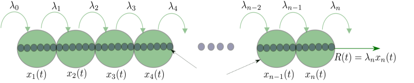
Figure 1: The RFM as a chain of $n$ sites of codons. Each site is described by a state variable $x_{i}(t)\in[0,1]$ expressing the normalized ribosome occupancy in site $i$ at time $t$. $\lambda_{0}$ is the initiation rate, and $\lambda_{i}$ is the elongation rate from site $i$ to site $(i+1)$. Production rate at time $t$ is $R(t):=\lambda_{n}x_{n}(t)$.

The dynamics of the RFM with $n$ sites is given by $n$ nonlinear first-order ordinary differential equations:

$$\dot{x}_{1} =\lambda_{0}(1-x_{1})-\lambda_{1}x_{1}(1-x_{2}),$$

$$\dot{x}_{2} =\lambda_{1}x_{1}(1-x_{2})-\lambda_{2}x_{2}(1-x_{3}),$$

$$\dot{x}_{3} =\lambda_{2}x_{2}(1-x_{3})-\lambda_{3}x_{3}(1-x_{4}),$$

$$\vdots$$

$$\dot{x}_{n-1} =\lambda_{n-2}x_{n-2}(1-x_{n-1})-\lambda_{n-1}x_{n-1}(1-x_{n}),$$

$$\dot{x}_{n} =\lambda_{n-1}x_{n-1}(1-x_{n})-\lambda_{n}x_{n}.$$ (2)

If we let $x_{0}(t):=1$ and $x_{n+1}(t):=0$, then (II) can be written more succinctly as

$$\dot{x}_{i}=h_{i-1}(x)-h_{i}(x),\quad i=1,\dots,n,$$ (3)

where $h_{i}(x):=\lambda_{i}x_{i}(1-x_{i+1})$. This can be explained as follows. The flow of particles from site $i$ to site $(i+1)$ at time $t$ is $\lambda_{i}x_{i}(1-x_{i+1})$. This flow increases with the density at site $i$, and decreases as site $(i+1)$ becomes fuller. This corresponds to a “soft” version of a simple exclusion principle: since the particles have volume, the input rate to site $i$ decreases as the number of particles in that site increases. Note that the maximal possible flow from site $i$ to site $(i+1)$ is the transition rate $\lambda_{i}$. Thus Eq. (3) simply states that the change in the density at site $i$ at time $t$ is the input rate to site $i$ (from site $i-1$) minus the output rate (to site $i+1$) at time $t$.

The ribosome exit rate from site $n$ at time $t$ is equal to the protein production (or translation) rate at time $t$, and is denoted by $R(t):=\lambda_{n}x_{n}(t)$ (see Fig. 1). Note that $x_{i}$ is dimensionless, and that every rate $\lambda_{i}$ has units of 1/time.

Let $x(t,a)$ denote the solution of (II) at time $t\geq 0$ for the initial condition $x(0)=a$. Since the state-variables correspond to normalized occupancy levels, we always assume that $a$ belongs to the closed $n$-dimensional unit cube:

$$C^{n}:=\{x\in\mathbb{R}^{n}:x_{i}\in[0,1],i=1,\dots,n\}.$$

Let $\operatorname{{\mathrm{i}nt}}(C^{n})$ denote the interior of $C^{n}$, and let $\partial C^{n}$ denote the boundary of $C^{n}$. It was shown in [34] that if $a\in C^{n}$ then $x(t,a)\in C^{n}$ for all $t\geq 0$, that is, $C^{n}$ is an invariant set of the dynamics. Ref. [34] also showed that the RFM is a tridiagonal cooperative dynamical system [52], and that this implies that (II) admits a unique steady-state point $e=e(\lambda_{0},\dots,\lambda_{n})\in\operatorname{{\mathrm{i}nt}}(C^{n})$, that is globally asymptotically stable, that is, $\lim_{t\to\infty}x(t,a)=e$, for all $a\in C^{n}$ (see also [31]). In particular, the production rate converges to the steady-state value $R:=\lambda_{n}e_{n}$.

An important advantage of the RFM (e.g. as compared to TASEP) is that it is amenable to mathematical analysis using various tools from systems and control theory. Furthermore, most of the analysis results hold for the general, nonhomogeneous case (i.e. when the transition rates all differ from one another). The RFM has been used to address many important biological problems including the sensitivity of the production rate to small changes in the transition rate, maximizing and minimizing the production rate in an optimal manner, analysis of the effect of competition for shared resources in translation, and more [33, 63, 34, 35, 31, 38, 39, 42, 62, 65, 41, 64].

To account for the fact that each ribosome covers several codons, we analyze here the RFMEO, which is a mean-field approximation of TASEPEO (see Appendix B for more details). An integer $\ell\geq 1$ describes the number of site units covered by each particle. The exclusion principle now implies that the rate of flow from site $i$ to site $(i+1)$ is $\lambda_{i}x_{i}(1-x_{i+1}-\cdots-x_{i+\ell})$. Indeed, since the particle covers the next $\ell$ sites, as the density in any of the $\ell$ consecutive sites increases the rate of movement slows down. Note that $\ell=1$ yields the RFM, so the RFM is a special case of the RFMEO.

Nevertheless, the RFMEO is a significant generalization of the RFM and its dynamics is quite different from that of the RFM. For example, the RFMEO, unlike the RFM, is not a cooperative system; it does not satisfy the particle-hole symmetry of the RFM (and of TASEP) [64, 4], and unlike the RFM, the RFMEO with $\ell>1$ is not a tridiagonal dynamical system.

III Ribosome Flow Model with Extended Objects (RFMEO)

Being a large complex of molecules, each ribosome typically covers between $10$ to $11$ codons and the geometry (e.g. length of the exit tunnel) can be longer than 30 codons [1]. A drawback of the RFM and other standard mean field models for translation is that, without additional processing such as coarse-graining, each ribosome (“particle”) is assumed to cover a single site.

The RFMEO allows modeling the flow of ribosomes where every ribosome covers $1\leq\ell\leq n$ site units. We assume, without loss of generality, that the ribosome is translating the left-most site it is covering, and refer to this part of the ribosome as the reader. A similar assumption is used in TASEPEO (see, for example, [14, 51, 50, 27, 49, 15]). Thus, the statement “the ribosome is at site $i$” means that: the reader is located at site $i$; the ribosome is translating site $i$; its corresponding transition rate is $\lambda_{i}$; and sites $i,\dots,i+\ell-1$, are covered by this ribosome. As we will show below, the dynamical equations describing the RFMEO (and thus all the theoretical results in this paper) are the same for any chosen reader location (e.g. choosing the reader at location $\ell/2$ results in exactly the same RFMEO equations).

Let $x_{i}(t)$ denote the (normalized) reader occupancy level at site $i$ at time $t$, and let $y_{i}(t)$ denote the (normalized) coverage occupancy level at site $i$ at time $t$, that is,

$$y_{i}(t):=\sum_{\mathclap{j=\max\{1,i-\ell+1\}}}^{i}x_{j}(t),\quad i=1,\dots,n.$$ (4)

Indeed, since every ribosome covers $\ell$ sites, any ribosome that is located up to $\ell$ sites left to site $i$ contributes to the total ribosome coverage at site $i$. The term “normalized” here means that each $x_{i}(t)$ and each $y_{i}(t)$ takes values in the interval $[0,1]$ for all $t\geq 0$. The value zero corresponds to completely empty, and one means completely full. We refer to $1-y_{i}(t)$ as the “space” or “vacancy” level at site $i$ at time $t$.

Note that (4) implies that $y(t)=Px(t)$, where $P$ is the lower triangular matrix with all entries zero, except for the entries on the main diagonal and $(\ell-1)$ diagonals below the main diagonal that are ones. For example, for $n=4$ and $\ell=3$:

$$P=\begin{bmatrix}1&0&0&0\\ 1&1&0&0\\ 1&1&1&0\\ 0&1&1&1\end{bmatrix}.$$ (5)

The dynamics of the RFMEO with $n$ sites is given by $n$ nonlinear first-order ordinary differential equations:

$$\dot{x}_{i}=q_{i-1}(x)-q_{i}(x),\quad i=1,\dots,n.$$ (6)

Here $q_{i-1}$ is the flow into site $i$ and $q_{i}$ is the flow out of site $i$. The expression for this flow is given by

$$q_{i}(x):=\lambda_{i}x_{i}(1-y_{i+\ell}),\quad i=0,\dots,n,$$ (7)

with $x_{0}(t)\equiv 1$, and $y_{j}(t)\equiv 0$ for all $j>n$.

Eq. (7) implies that the reader flow from site $i$ to site $(i+1)$ is proportional to $\lambda_{i}$, to the occupancy levels of readers at site $i$, and to the “space” or “vacancy” level at site $i+\ell$ (see Fig. 2). In particular,

• As the number of readers at site $i$ increases, the flow from site $i$ increases. This follows the same reasoning as in the RFM.

• When a reader located at site $i$ moves to site $(i+1)$, the coverage occupancies at sites $i+1,i+2,\dots,i+\ell-1$ do not change. However, the reader’s tail end will now occupy a new site, which is site $(i+\ell)$.

• The “vacancy” level at site $(i+\ell)$ is $(1-y_{i+\ell})$, since $y_{i+\ell}$ denotes the total coverage at site $(i+\ell)$.

To explain (6), consider for example the equation for the change in the density at site $1$ given by

$$\dot{x}_{1} =q_{0}(x)-q_{1}(x)$$

$$=\lambda_{0}(1-y_{\ell})-\lambda_{1}x_{1}(1-y_{\ell+1}).$$

The term $\lambda_{0}(1-y_{\ell})$ represents the entry rate into site $1$. Indeed, since the entering ribosome will cover sites $1,2,\dots,\ell$, this entry rate decreases with the coverage density $y_{\ell}=x_{1}+\dots+x_{\ell}$. (In the literature on TASEPEO this is referred to as the “complete-entry” flow [14]). The term $\lambda_{1}x_{1}(1-y_{\ell+1})$ is the flow from site $1$ to site $2$. This increases with the occupancy at site $1$ and, similarly, decreases with the coverage occupancy $y_{\ell+1}$.

Remark 1

As noted above, the assumption that the “reading head” is located at the left hand-side of the ribosome is arbitrary, but the RFMEO equations do not depend on this assumption. To demonstrate this, consider for example the case $\ell=3$ and the three possible locations for the reader: (1) Left-most site. In this case $y_{j}=x_{j-2}+x_{j-1}+x_{j}$, so

$$q_{i}(x)=\lambda_{i}x_{i}(1-y_{i+3})=\lambda_{i}x_{i}(1-x_{i+1}-x_{i+2}-x_{i+3});$$ (8)

(2) Middle site. In this case $y_{j}=x_{j-1}+x_{j}+x_{j+1}$, and $q_{i}(x)=\lambda_{i}x_{i}(1-y_{i+2})$, and this yields (8); (3) Right-most site. In this case $y_{j}=x_{j}+x_{j+1}+x_{j+2}$, and $q_{i}(x)=\lambda_{i}x_{i}(1-y_{i+1})$, again yielding (8). Thus (7) is invariant to the reader location.

Consider an index $j\geq n-\ell+2$. Then $\ell+j-1\geq n+1$, so

$$\dot{x}_{j} =q_{j-1}(x)-q_{j}(x)$$

$$=\lambda_{j-1}x_{j-1}(1-y_{\ell+j-1})-\lambda_{j}x_{j}(1-y_{\ell+j})$$

$$=\lambda_{j-1}x_{j-1}-\lambda_{j}x_{j}.$$

Thus, the equation describing the flow in these last sites is a linear equation. The same phenomena takes place in TASEPEO, as a ribosome “reading” the last $\ell$ codons must be the last particle on the lattice, with no others to impede its progress. Therefore, it can move without hindrance toward the exit end. The exit rate in this context is referred to as the “incremental-exit” rate [14].

The output rate of ribosomes from the chain, which is the protein production (or translation) rate, is denoted by $R(t):=\lambda_{n}x_{n}$.

Note that in the special case $\ell=1$ we have $y_{i}=x_{i}$ for all $i=1,\dots,n$, and then (6) reduces to the RFM.

Example 1

Consider a RFMEO with dimension $n=4$ and particle size $\ell=2$. Then (6) yields

$$\dot{x}_{1} =\lambda_{0}(1-y_{2})-\lambda_{1}x_{1}(1-y_{3}),$$

$$=\lambda_{0}(1-x_{1}-x_{2})-\lambda_{1}x_{1}(1-x_{2}-x_{3}),$$

$$\dot{x}_{2} =\lambda_{1}x_{1}(1-y_{3})-\lambda_{2}x_{2}(1-y_{4}),$$

$$=\lambda_{1}x_{1}(1-x_{2}-x_{3})-\lambda_{2}x_{2}(1-x_{3}-x_{4}),$$

$$\dot{x}_{3} =\lambda_{2}x_{2}(1-y_{4})-\lambda_{3}x_{3},$$ (9)

$$=\lambda_{2}x_{2}(1-x_{3}-x_{4})-\lambda_{3}x_{3},$$

$$\dot{x}_{4} =\lambda_{3}x_{3}-\lambda_{4}x_{4}.$$

In the RFM the set $C^{n}$ is an invariant set of the dynamics. This is no longer true for the RFMEO. For example for the initial condition

$$x(0)=\begin{bmatrix}1&0.1&1&1\end{bmatrix}^{\prime},$$ (10)

Eq. (1) yields

$$\dot{x}_{1}(0)=0.1(\lambda_{1}-\lambda_{0}).$$

This implies that $x_{1}(0^{+})>1$ for $\lambda_{1}>\lambda_{0}$, so $x(0^{+})\not\in C^{n}$. $\square$

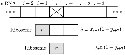
Figure 2: Schematic explanation of the RFMEO with $\ell=3$. Ribosomes that cover three sites scan the mRNA from left-to-right. The label $r$ denotes the reader location. Shown are the two terms affecting the occupancy level at site $i$ in the RFMEO dynamics (see (7) and (6)).

Remark 2

The Jacobian matrix of the dynamics (1) is

$$J(x)=\begin{bmatrix}-\lambda_{0}-\lambda_{1}(1-x_{2}-x_{3})&-\lambda_{0}+\lambda_{1}x_{1}&\lambda_{1}x_{1}&0\\ \lambda_{1}(1-x_{2}-x_{3})&-\lambda_{1}x_{1}-\lambda_{2}(1-x_{3}-x_{4})&-\lambda_{1}x_{1}+\lambda_{2}x_{2}&\lambda_{2}x_{2}\\ 0&\lambda_{2}(1-x_{3}-x_{4})&-\lambda_{2}x_{2}-\lambda_{3}&-\lambda_{2}x_{2}\\ 0&0&\lambda_{3}&-\lambda_{4}\end{bmatrix}.$$

Note that there are off-diagonal entries here whose sign may change with time (e.g. $-\lambda_{0}+\lambda_{1}x_{1}$). This implies that the RFMEO, unlike the RFM, is not a cooperative dynamical system.

It is useful to explicitly write the dynamics of the RFMEO in terms of the coverage state-variables (i.e. the $y$ state-vector). Recall that the proofs of all the results are placed in Appendix A.

Proposition 1

The coverage state-variables in the RFMEO satisfy:

$$\dot{y}_{i}= \lambda_{0}(1-y_{\ell})-\lambda_{i}\left(\sum_{k=0}^{\lceil(i-\ell)/\ell\rceil}(y_{i-k\ell}-y_{i-k\ell-1})\right)(1-y_{i+\ell}), \quad 1\leq i\leq\ell,$$

$$\dot{y}_{i}= \lambda_{i-\ell}\left(\sum_{k=0}^{\lceil((i-\ell)/\ell)-1\rceil}(y_{i-(k+1)\ell}-y_{i-(k+1)\ell-1})\right)(1-y_{i})$$

$$-\lambda_{i}\left(\sum_{k=0}^{\lceil(i-\ell)/\ell\rceil}(y_{i-k\ell}-y_{i-k\ell-1})\right)(1-y_{i+\ell}), \quad\ell<i\leq n,$$ (11)

where $\lceil z\rceil$ denotes the smallest integer that is larger than or equal to $z$.

Example 2

Consider the RFMEO with $n=4$ sites and particle size $\ell=2$. Then (1) yields

$$\dot{y}_{1} =\lambda_{0}(1-y_{2})-\lambda_{1}y_{1}(1-y_{3}),$$

$$\dot{y}_{2} =\lambda_{0}(1-y_{2})-\lambda_{2}(y_{2}-y_{1})(1-y_{4}),$$

$$\dot{y}_{3} =\lambda_{1}y_{1}(1-y_{3})-\lambda_{3}(y_{3}-y_{2}+y_{1}),$$

$$\dot{y}_{4} =\lambda_{2}(y_{2}-y_{1})(1-y_{4})-\lambda_{4}(y_{4}-y_{3}+y_{2}-y_{1}).~{}\square$$

IV Theoretical Results

We begin by defining the relevant state-space for the RFMEO. If for some $i$ we have $y_{i+\ell}>1$ then $q_{i}(x):=\lambda_{i}x_{i}(1-y_{i+\ell})<0$. This represents a backward flow that according to current knowledge does not take place in ribosome movement. Thus, it is useful to define the state-space as the region where such a backward flow does not take place, i.e. both the $x_{i}$s and the $y_{i}$s are between zero and one. This leads to defining

$$H:=\{x\in\mathbb{R}^{n}:x\in C^{n}\text{ and }Px\in C^{n}\}.$$

Note that $H$ is a compact and convex set.

Example 3

Consider the RFMEO with $n=3$ sites and particle size $\ell=2$. The sets $H$ and $C^{3}$ are depicted in Fig. 3. $\square$

Note also that for the RFMEO with $n=4$ and $\ell=2$ the initial condition $x(0)$ in (10) is not in $H$ as $y_{2}(0)=x_{1}(0)+x_{2}(0)>1$.

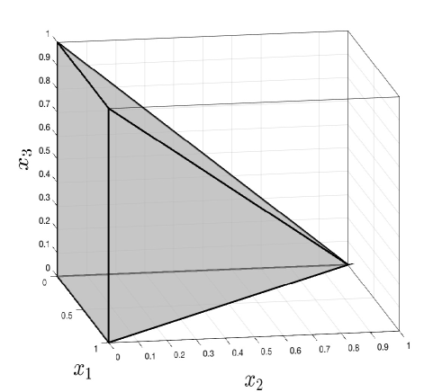
Figure 3: RFMEO with $n=3$ sites and particle size $\ell=2$. Gray volume is $H$, and the white cube is $C^{3}$.

From here on we refer to any value $x\in H$ as a feasible value. This represents a state such that every reader density and every coverage density is between zero and one.

IV-A Invariance and persistence

The next result shows that the boundary of $H$, denoted $\partial H$, is “repelling” towards the interior of $H$. This means that if the dynamics is initiated with a feasible value that includes a reader/coverage density equal to the extremal value zero [one] then the dynamics will immediately change this to a value larger than zero [smaller than one].

Proposition 2

For any $a\in\partial H$ the solution of the RFMEO satisfies $x(t,a)\in\operatorname{{\mathrm{i}nt}}(H)$ for all $t>0$.

Note that this result implies in particular that $H$ is an invariant set of the dynamics. In other words, if all the reader and coverage densities are initiated with feasible values (i.e. values between zero and one) at time $t=0$ then they remain feasible for all time $t\geq 0$.

The next result shows that the solutions of the RFMEO are “persistent” in the sense that they enter and remain in a set that is uniformly separated from the boundary of $H$. Furthermore, this happens “immediately”.

Proposition 3

For any $\tau>0$ there exists a compact and convex set $H_{\tau}$ that is strictly contained in $H$ such that for any $a\in H$,

$$x(t,a)\in H_{\tau},\text{ for all }t\geq\tau.$$

Note that this implies that for any $\tau>0$ there exists $\delta=\delta(\tau)\in(0,1/2)$ such that

$$x_{i}(t,a),y_{i}(t,a)\in[\delta,1-\delta],\text{ for all }t\geq\tau,$$

for all $i$ and all $a\in H$. In other words, all the reader and coverage densities “immediately” become and remain uniformly separated from the extreme values zero and one. This is a technical property, but as we will see below it will be useful in the analysis of the asymptotic properties of the RFMEO.

IV-B Contraction

Contraction theory is a powerful tool for analyzing nonlinear dynamical systems. In a contractive system, trajectories that emanate from different initial conditions approach each other at an exponential rate, that is, the distance between any pair of trajectories, as a function of time, decreases at an exponential rate [28, 45, 2].

Consider the time-varying dynamical system

$$\dot{x}(t)=f(t,x(t)),$$ (12)

whose trajectories evolve on a compact and convex set $\Omega\subset\mathbb{R}^{n}$.

For $t\geq t_{0}\geq 0$, and $a\in\Omega$, let $x(t,t_{0},a)$ denote the solution of (12) at time $t$ for the initial condition $x(t_{0})=a$. Recall that system (12) is said to be contartive on $\Omega$ w.r.t. a norm $|\cdot|:\mathbb{R}^{n}\to\mathbb{R}_{+}$ if there exists $\gamma>0$ such that

$$|x(t_{2},t_{1},a)-x(t_{2},t_{1},b)|\leq\exp(-(t_{2}-t_{1})\gamma)|a-b|$$ (13)

for all $t_{2}\geq t_{1}\geq 0$ and all $a,b\in\Omega$. This means that any two trajectories approch each other at an exponential rate $\gamma$.

To apply contraction theory to the RFMEO, we require the following generalization of contraction with respect to a fixed norm that has been introduced in [32]. The time-varying system (12) is said to be contractive after a small overshoot and short transient (SOST) on $\Omega$ w.r.t. a norm $|\cdot|:\mathbb{R}^{n}\to\mathbb{R}_{+}$ if for each $\varepsilon>0$ and each $\tau>0$ there exists $\gamma=\gamma(\tau,\varepsilon)>0$ such that

$$|x(t_{2}+\tau, t_{1},a)-x(t_{2}+\tau,t_{1},b)|\leq(1+\varepsilon)\exp(-(t_{2}-t_{1})\gamma)|a-b|\,$$

for all $t_{2}\geq t_{1}\geq 0$ and all $a,b\in\Omega$. Comparing this to (13), we see that here contraction “kicks in” after an arbitrarily small time transient $\tau$ and with an arbitrarily small overshoot $(1+\varepsilon)$.

The next result applies these ideas to the RFMEO. Let $|\cdot|_{1}:\mathbb{R}^{n}\to\mathbb{R}_{+}$ denote the $L_{1}$ norm, i.e. for $z\in\mathbb{R}^{n}$, $|z|_{1}=|z_{1}|+\dots+|z_{n}|$.

Proposition 4

The RFMEO is SOST on $H$ w.r.t. the $L_{1}$ norm, that is, for each $\varepsilon>0$ and each $\tau>0$ there exists $\gamma=\gamma(\tau,\varepsilon)>0$ such that

$$|x(t+\tau,a)-x(t+\tau,b)|_{1}\leq(1+\varepsilon)\exp(-\gamma t)|a-b|_{1}\,$$ (14)

for all $t\geq 0$ and all $a,b\in H$.

Roughly speaking, this means the following. Fix two initial feasible densities in the RFMEO and consider how the two corresponding densities along the mRNA evolve in time. Then these densities become “more similar” to each other at an exponential rate. In particular, the initial density is “quickly forgotten”.

Subsections IV-C and IV-E below describe important asymptotic properties of the RFMEO that follow from Prop. 4.

IV-C Global asymptotic stability

Write the RFMEO (6) as $\dot{x}=g(x)$, with $g:H\to\mathbb{R}^{n}$. Since the compact and convex set $H$ is an invariant set of this dynamical system, it contains a steady-state point $e=e(\lambda_{0},\dots,\lambda_{n})$. In other words, $g(e)=0_{n}$, where $0_{n}$ denotes a column vector of $n$ zeros, and $x(t,e)\equiv e$ for all $t\geq 0$. Prop. 2 implies that $e\in\operatorname{{\mathrm{i}nt}}(H)$. Using (14) with $b:=e$ yields the following result.

Corollary 1

The RFMEO admits a globally asymptotically stable steady-state point $e\in\operatorname{{\mathrm{i}nt}}(H)$, i.e.

$$\lim_{t\to\infty}x(t,a)=e,\text{ for all }a\in H.$$

This means that trajectories corresponding to different initial conditions all converge to the unique steady-state point, that depends on the transition rates $\lambda_{i}$s, particle size $\ell$, and the length of the chain $n$, but not on the initial condition.

Example 4

Fig. 4 depicts the trajectories of an RFMEO with dimension $n=3$, particle size $\ell=2$, and rates $\lambda_{0}=1.0$, $\lambda_{1}=1.2$, $\lambda_{2}=0.8$, and $\lambda_{3}=0.4$, for four different initial conditions on the boundary of $H$. It may be seen that each trajectory immediately enters and remains in the interior of $H$, and converges to a unique steady-state point $e\in\operatorname{{\mathrm{i}nt}}(H)$. $\square$

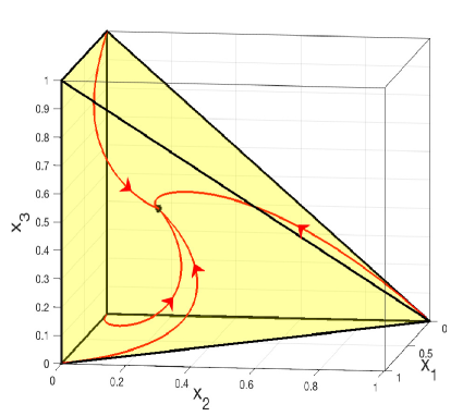
Figure 4: Four trajectories of the RFMEO with $n=3$, $\ell=2$, $\lambda_{0}=1.0$, $\lambda_{1}=1.2$, $\lambda_{2}=0.8$, and $\lambda_{3}=0.4$. The unique steady-state point $e\in\operatorname{{\mathrm{i}nt}}(H)$ is marked by a black dot.

The next example demonstrates the contraction property. Let $1_{n}$ denote the column vector of $n$ ones.

Example 5

Consider the RFMEO with dimension $n=7$, particle size $\ell=3$, and rates $\lambda_{i}=1-\frac{i}{50}$, $i=0,\dots,7$. In this case the unique steady-state point is (all numbers are to four digit accuracy):

$$e=\begin{bmatrix}0.3896&0.2697&0.2262&0.2042&0.1272&0.1302&0.1331\end{bmatrix}^{\prime}.$$

Fig. 5 depicts $r(t):=|x(t,a)-e|_{1}$ as a function of time for $t\in[0,70]$ for the initial condition $a=(3/20)1_{7}$. It may be seen that the $L_{1}$ distance between the trajectory and $e$ monotonically decreases to zero. It may also be seen that the rate of convergence varies with time. This makes sense because we can interpret the RFMEO as an RFM with time-varying transition rates (see the proof of Prop. 4 in Appendix A), and thus a time-varying contraction rate. $\square$

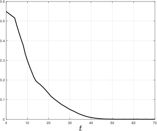
Figure 5: The distance $|x(t,a)-e|_{1}$ as a function of $t$ for the RFMEO in Example 5.

Corollary 1 implies that the coverage occupancy $y_{i}(t)$ at site $i$ converges to the unique steady-state value:

$$z_{i}:=\sum_{\mathclap{j=\max\{1,i-\ell+1\}}}^{i}e_{j},\quad i=1,\dots,n.$$ (15)

Define the mean reader occupancy at time $t$ by $\rho(t):=\frac{1}{n}{\sum_{i=1}^{n}x_{i}(t)},$ and the mean coverage occupancy at time $t$ by $\rho^{c}(t):=\frac{1}{n}{\sum_{i=1}^{n}y_{i}(t)}.$ Note that this implies that $\lim_{n\to\infty}\rho^{c}(t)=\ell\rho(t)$. Then the mean reader occupancy converges to the unique steady-state value

$$\rho:=\frac{1}{n}{\sum_{i=1}^{n}e_{i}},$$ (16)

and the mean coverage occupancy converges to the unique steady-state value

$$\rho^{c}:=\frac{1}{n}\sum_{i=1}^{n}z_{i}.$$ (17)

The next example demonstrates the contraction property using a S. Cerevisiae gene. Let $0_{n}$ denote the column vector of $n$ zeros.

Example 6

We consider the highly-expressed S. Cerevisiae gene YLR110C that encodes a cell wall mannoprotein, and contains $133$ codons (excluding the stop codon). We modeled it using a RFMEO with $n=133$ and $\ell=10$. The value $\lambda_{0}=1.33131$ [in units of mRNAs/sec] was estimated based on the ribosome density per mRNA levels, as this value is expected to be approximately proportional to the initiation rate when initiation is rate limiting [43, 33]. The elongation rates $\lambda_{1},\dots,\lambda_{n}$, were estimated using ribo-seq data for the codon decoding rates [11], normalized so that the median elongation rate of all S. cerevisiae mRNAs becomes $6.4$ codons per second [24]. The rates are depicted in the top panel of Fig. 6 as a function of $i$. To study the rate of contraction, we calculated $e$ in the RFMEO (shown in the middle panel of Fig. 6), and simulated the dynamical system to obtain $r(t)=|x(t,a)-e|_{1}$ with $a=0_{133}$, as a function of $t$ [in seconds]. Note that the initial condition $a=0_{133}$ represents an mRNA with no ribosomes. The bottom panel of Fig. 6 depicts the relative $L_{1}$ distance in percentage, that is,

$$100\frac{r(t)}{r(0)},$$ (18)

as a function of $t$ [in seconds]. In this case, $\rho=0.0534$. It may be seen that the relative distance is less than $20\%$ already after about $30$ seconds. We note that typical S. Cerevisiae mRNAs half-lives is in the order of tens of minutes (see, for example, [48, 61, 17]). This suggests that typically the ribosome density on S. Cerevisiae mRNAs is “very close” to its steady-state value.

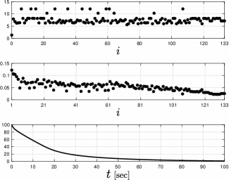
Figure 6: The biological model in Example 6. Top: $\lambda_{i}$ as a function of $i$; Middle: steady-state reader density $e_{i}$ as a function of $i$; Bottom: relative $L_{1}$ distance in percentage (see (18)) as a function of $t$.

IV-D Analysis of the steady-state

It is important to understand how the steady-state density $e$ depends on the parameters of the RFMEO. To study this we begin by deriving some equations for $e$. At steady-state (i.e. for $x=e$), the left-hand side of all the equations in (6) is zero (i.e. $\dot{x}_{i}=0$, $i=1,\dots,n$), so

$$R=q_{i}(e)=\lambda_{i}e_{i}(1-z_{i+\ell}),\quad i=0,\dots,n,$$

where $z_{j}:=0$, for all $j>n$. This yields (see (15))

$$\lambda_{0}(1-e_{1}-\dots-e_{\ell}) =\lambda_{1}e_{1}(1-e_{2}-\dots-e_{\ell+1})$$

$$=\lambda_{2}e_{2}(1-e_{3}-\dots-e_{\ell+2})$$

$$\vdots$$

$$=\lambda_{n-\ell-1}e_{n-\ell-1}(1-e_{n-\ell}-\dots-e_{n-1})$$

$$=\lambda_{n-\ell}e_{n-\ell}(1-e_{n-\ell+1}-\dots-e_{n})$$

$$=\lambda_{n-\ell+1}e_{n-\ell+1}$$

$$\vdots$$

$$=\lambda_{n}e_{n}$$

$$=R.$$ (19)

We can express these in terms of the (generally unknown value) $R$ as:

$$e_{i}=\frac{R\lambda_{i}^{-1}}{1-e_{i+1}-e_{i+2}-\dots-e_{i+\ell}}=\frac{e_{n}\lambda_{n}\lambda_{i}^{-1}}{1-e_{i+1}-e_{i+2}-\dots-e_{i+\ell}},$$ (20)

and this yields

$$e_{n-j} =R\lambda_{n-j}^{-1},\quad\quad\quad j=0,\dots,\ell-1,$$

$$e_{n-\ell} =\frac{R\lambda_{n-\ell}^{-1}}{1-R\sum_{k=0}^{\ell-1}\lambda_{n-k}^{-1}},$$

$$e_{n-\ell-1} =\cfrac{R\lambda_{n-\ell-1}^{-1}}{1-\cfrac{R\lambda_{n-\ell}^{-1}}{1-R\sum_{k=0}^{\ell-1}\lambda_{n-k}^{-1}}-R\sum_{k=1}^{\ell-1}\lambda_{n-k}^{-1}},$$

$$\vdots$$

and

$$0=1-\frac{R\lambda_{0}^{-1}}{1-e_{1}-\dots-e_{\ell}}.$$

Example 7

Consider the RFMEO with dimension $n=6$ and particle size $\ell=3$. Then, the steady-state production rate $R$ satisfies

$$0=1-\frac{R\lambda_{0}^{-1}}{1-e_{1}-e_{2}-e_{3}},$$

where

$$e_{1} =\cfrac{R\lambda_{1}^{-1}}{1-\cfrac{R\lambda_{2}^{-1}}{1-\cfrac{R\lambda_{3}^{-1}}{1-R(\lambda_{4}^{-1}+\lambda_{5}^{-1}+\lambda_{6}^{-1})}-R(\lambda_{4}^{-1}+\lambda_{5}^{-1})}-\cfrac{R\lambda_{3}^{-1}}{1-R(\lambda_{4}^{-1}+\lambda_{5}^{-1}+\lambda_{6}^{-1})}-R\lambda_{4}^{-1}},$$

$$e_{2} =\cfrac{R\lambda_{2}^{-1}}{1-\cfrac{R\lambda_{3}^{-1}}{1-R(\lambda_{4}^{-1}+\lambda_{5}^{-1}+\lambda_{6}^{-1})}-R(\lambda_{4}^{-1}+\lambda_{5}^{-1})},$$

$$e_{3} =\cfrac{R\lambda_{3}^{-1}}{1-R(\lambda_{4}^{-1}+\lambda_{5}^{-1}+\lambda_{6}^{-1})}.~{}\square$$

It is clear that solving (IV-D) is in general non-trivial. Nevertheless, it can be solved in closed-form in some very special cases. The next example demonstrates this.

Example 8

Consider a RFMEO with $n$ sites and with ribosome size $\ell=n$. Then (IV-D) becomes

$$\lambda_{0}(1-e_{1}-\dots-e_{n}) =\lambda_{1}e_{1}$$

$$=\lambda_{2}e_{2}$$

$$\vdots$$

$$=\lambda_{n}e_{n}$$

$$=R,$$ (21)

and this yields

$$e_{i}=\frac{1}{z}\prod_{\begin{subarray}{c}j=0\\ j\not=i\end{subarray}}^{n}\lambda_{j},\quad i=1,\dots,n,$$ (22)

and

$$R=\frac{1}{z}\prod_{j=0}^{n}\lambda_{j},$$ (23)

where $z:=\sum_{0\leq i_{1}<i_{2}<\dots<i_{n}\leq n}\lambda_{i_{1}}\lambda_{i_{2}}\dots\lambda_{i_{n}}$. To understand this, assume in addition that $\lambda_{0}=\dots=\lambda_{n}=\lambda_{c}$, i.e. all the rates are equal with $\lambda_{c}$ denoting the common value. Then (22) and (23) yield $e_{i}=1/(n+1)$ for all $i$, and

$$R=\lambda_{c}/(n+1).$$ (24)

This means that when the ribosome size is equal to the chain size and all the rates are equal then the steady-state density at each site is identical. This makes sense, as every ribosome covers all the sites in the chain.

Another tractable case is when $\ell=n-1$ and $\lambda_{0}=\dots=\lambda_{n}=\lambda_{c}$. Then (IV-D) yields

$$\lambda_{c}(1-e_{1}-\dots-e_{n-1}) =\lambda_{c}e_{1}(1-e_{2}-\dots-e_{n})$$

$$=\lambda_{c}e_{2}$$

$$\vdots$$

$$=\lambda_{c}e_{n}$$

$$=R,$$ (25)

and this admits the solution

$$e_{1}=\frac{2}{\sqrt{4n-3}+1},\quad e_{i}=\frac{2}{\sqrt{4n-3}+2n-1}\text{ for all }i>1,$$

and

$$R=\frac{2\lambda_{c}}{\sqrt{4n-3}+2n-1}.$$ (26)

Note that here $e_{1}>e_{2}=e_{3}=\dots=e_{n}$. This makes sense, because if there is a ribosome with reader at site $\geq 2$ then the tail of this $(n-1)$-sites long ribosome is either at site $n$ or already out of the chain, and so there is no hindrance for its movement. $\square$

Eq. (IV-D) can also be used to prove theoretical results. The next result shows that increasing any of the $\lambda_{i}$s increases $R$. In other words, increasing any of the transition rates along the mRNA molecule increases the steady-state protein production rate.

Proposition 5

Consider the RFMEO with dimension $n$ and particle size $\ell$. Then $\frac{\partial}{\partial\lambda_{i}}R>0$, for $i=0,\dots,n$.

In the special case where all the rates are equal, i.e.

$$\lambda_{0}=\cdots=\lambda_{n}:=\lambda_{q},$$ (27)

where $\lambda_{q}$ denotes the common value, we refer to the RFMEO as the totally homogeneous RFMEO (THRFMEO). In this case, it is possible to say more about the steady-state occupancies.

Proposition 6

Consider the THRFMEO with dimension $n$ and particle size $\ell$. Then

$$e_{1}>e_{2}>\cdots>e_{n-\ell+1},$$

$$e_{n-\ell+1}=e_{n-\ell+2}=\cdots=e_{n},$$

$$z_{\ell}>z_{\ell+1}>\cdots>z_{n}.$$ (28)

This means that the steady-state reader occupancies monotonically decrease between sites $1$ and $(n-\ell+1)$ and are equal at the last $\ell$ sites. This may partially explain the decrease in ribosome density observed along the coding sequences from the 5’ end to the 3’ end (see, for example, [9, 21]).

Example 9

The steady-state reader occupancy levels of the RFMEO with dimension $n=40$ are depicted in Fig. 7 for three particle sizes: $\ell=1$ (corresponding to the RFM), $\ell=2$, and $\ell=3$. It may be observed that the steady-state reader occupancies monotonically decrease along the chain until the last $\ell$ densities that are equal. The corresponding steady-state production rates are $R=0.2513$ for $\ell=1$; $R=0.1265$ for $\ell=2$; and $R=0.0851$ for $\ell=3$. $\square$

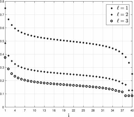
Figure 7: Steady-state reader occupancy level $e_{i}$ as a function of $i=1,\dots,40$, for a THRFMEO with $n=40$ sites, and with $\ell=1$ (*), $\ell=2$ (+), and $\ell=3$ (O).

IV-D1 Effect of particle size

It is interesting to analyze how the steady-state occupancies and production rate depend on the particle size $\ell$. One might naturally expect the steady-state production rate in the RFMEO to decrease as the particle size $\ell$ increases. Indeed, roughly speaking one may think of increasing the particle size as replacing small cars traveling along a unidirectional traffic lane with large trucks thus leading to more congestion. This is demonstrated by the next example.

Example 10

The steady-state reader occupancy levels in the RFMEO with dimension $n=60$, and rates $\lambda_{0}=\cdots=\lambda_{40}=1$, and $\lambda_{41}=\cdots=\lambda_{60}=1/5$, for four different particle sizes: $\ell=1$ (i.e. the RFM), $\ell=2$, $\ell=4$, and $\ell=8$ are depicted in Fig. 8. Note that the steady-state occupancy levels decrease with $\ell$. The transition rates here decrease from the value $1$ to $1/5$ at site $40$. Thus, we except to see a “traffic jam” of ribosomes before this site. For $\ell=1$ this is indeed what happens. However, for $\ell>1$ much more complicated patterns evolve. The steady-state densities follow a complicated quasi-periodic behavior, with period $\ell$, even though there is no such periodicity in the rates. $\square$

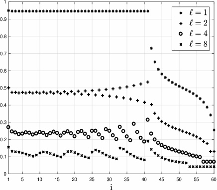
Figure 8: Steady-state reader occupancy level $e_{i}$ as a function of $i=1,\dots,60$, for a RFMEO with $n=60$, $\lambda_{0}=\cdots=\lambda_{40}=1$, and $\lambda_{41}=\cdots=\lambda_{60}=1/5$, with $\ell=1$ (*), $\ell=2$ (+), $\ell=4$ (O), and $\ell=8$ (x).

Example 11

Fig. 9 depicts the steady-state production rate $R$, the steady-state mean reader occupancy $\rho$, and the steady-state mean coverage occupancy $\rho^{c}$ as a function of the particle size $\ell$, for a THRFMEO with dimension $n=100$ and $\lambda_{q}=1$. It can be observed that the steady-state production rate and the mean reader occupancy decrease with $\ell$, whereas the steady-state mean coverage occupancy increases with $\ell$.

It is interesting to compare these results to the homogeneous TASEPEO. In the thermodynamical limit (i.e. as $N\to\infty$), the homogeneous TASEPEO with particle size $\ell$, and with $\alpha=\beta=1$ is in the maximal current phase, where the steady-state output rate is $J=1/(1+\sqrt{\ell})^{2}$, the mean reader density is $1/(\sqrt{\ell}(1+\sqrt{\ell}))$, and the mean coverage density is $\sqrt{\ell}/(1+\sqrt{\ell)}$ [50, 14]. Note that this implies that as $\ell$ goes to infinity the current and the mean reader density go to zero, whereas the mean coverage density goes to one. This is consistent with the results for the THRFMEO depicted in Fig. 9.

Fig. 10 depicts the steady-state production rate $R$ as a function of the particle size $\ell$ for a RFMEO with $n=100$, $\lambda_{0}=0.1$, and $\lambda_{i}=1$, $i=1,\dots,100$. In this case $\lambda_{0}$ is the rate limiting factor, and thus less “traffic jams” occur relative to the case $\lambda_{0}=1$. It may be seen that also in this case $R$ monotonically decreases with $\ell$. $\square$

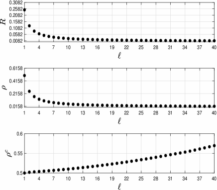
Figure 9: Steady-state production rate $R$, mean reader occupancy $\rho$, and mean coverage occupancy $\rho^{c}$ as a function of $\ell$, for a THRFMEO with $n=100$ sites and $\lambda_{q}=1$.

Figure 10: The steady-state production rate $R$ as a function of $\ell$, for a RFMEO with $n=100$, $\lambda_{0}=0.1$, and $\lambda_{i}=1$, $i=1,\dots,100$.

The next result shows that for fixed rates the steady-state production rate in the RFMEO with $\ell>1$ is always smaller than the steady-state production rate in the RFMEO with $\ell=1$ (i.e. the RFM).

Proposition 7

Consider an RFMEO with dimension $n$, particle size $\ell>1$, and rates $\lambda_{i}$, $i=0,\dots,n$, admitting a steady-state production rate $R$. Consider also an RFM with the same dimension $n$, and the same rates $\lambda_{i}$, $i=0,\dots,n$, admitting a steady-state production rate $\bar{R}$. Then $R<\bar{R}$.

In many organisms longer genes have lower protein levels [10, 18]. There are many explanations and variables that may contribute to this correlation. However, is it possible that the relations between particle size and translation rate may have a (small) contribution to this correlation? It is possible that longer coding regions are related to longer proteins emerging from the ribosome during translation thus practically increasing the effective ribosome size. This hypothesis may be studied in synthetic system in the future.

Surprisingly, however, increasing $\ell$ does not always lead to a reduction in the production rate.

Example 12

Consider an RFMEO with dimension $n=3$, and rates

$$\lambda_{0}=1.2,\;\lambda_{1}=0.8,\;\lambda_{2}=1.1,\;\lambda_{3}=3.$$

We consider two cases $\ell=2$ and $\ell=3$, and for the sake of clarity we denote the steady-state values in the latter case by overbars. For $\ell=2$,

$$e=\begin{bmatrix}0.5213&0.2498&0.0916\end{bmatrix}^{\prime},\text{ and }R=0.2749.$$

For $\ell=3$,

$$\bar{e}=\begin{bmatrix}0.3759&0.2733&0.1003\end{bmatrix}^{\prime},\text{ and }\bar{R}=0.3001.$$

Thus, here increasing $\ell$ from $2$ to $3$ increases the production rate. To explain this, recall that in general increasing $\ell$ decreases the steady-state reader densities (see Figs. 7 and 8). This is also what happens here. Indeed,

$$\bar{e}_{1}+\bar{e}_{2}+\bar{e}_{3}=0.7495<e_{1}+e_{2}=0.7711.$$

At steady-state, the entry rate into the chain is equal to the production rate, so $R=\lambda_{0}(1-e_{1}-e_{2})$ and $\bar{R}=\lambda_{0}(1-\bar{e}_{1}-\bar{e}_{2}-\bar{e}_{3})$. Since this is proportional to one minus the sum of densities, $\bar{R}>R$. Thus, in this particular case the increase in $\ell$ yields an increase in the production rate.

Similarly, it follows from (24) and (26) that for any $n>3$ increasing $\ell$ from $n-1$ to $n$ in the THRFMEO leads to an increase in the steady-state production rate. $\square$

IV-E Entrainment

Assume now that some or all of the transition rates $\lambda_{i}$ are not constants, but time-varying periodic functions with a common period $T$. In the context of translation, this corresponds for example to the case where the tRNA abundances vary in a periodic manner, with a common period $T$. More precisely, we say that a function $f$ is $T$-periodic if $f(t+T)=f(t)$ for all $t$. Assume that the transition rates are time-varying functions satisfying:

1. There exist $\delta_{1},\delta_{2}\in\mathbb{R}_{++}$ such that $0<\delta_{1}\leq\lambda_{i}(t)\leq\delta_{2}$, for all $i=0,\dots,n$, and all $t\geq 0$.

2. There exists a minimal $T>0$ such that every $\lambda_{i}(t)$ is a $T$-periodic function.

We refer to this case as the periodic RFMEO (PRFMEO). Note that the PRFMEO includes in particular the case where some of the rates are constant, as a constant function is $T$-periodic for every $T$. However, condition $2)$ above implies that the case where all the rates are constant is ruled out, as then the minimal $T$ is zero. Indeed, this case is just the RFMEO analyzed above.

The next result follows from combining the fact that the RFMEO is SOST on $H$ with known results on the entrainment of contractive systems to a periodic excitation (see e.g. [45]).

Theorem 1

The PRFMEO admits a unique function $\phi(\cdot):\mathbb{R}_{+}\to\operatorname{{\mathrm{i}nt}}(H)$, that is $T$-periodic, and for any $a\in H$ the trajectory $x(t,a)$ converges to $\phi$ as $t\to\infty$.

In other words, the PRFMEO admits a unique periodic solution, with period $T$, and every trajectory of the PRFMEO converges to this periodic solution. This means that the densities along the mRNA, and thus also the production rate entrain to the periodic excitation induced by the transition rates.

As a side note, we point that the RFMEO can also be used to model vehicular traffic. If traffic lights that change periodically produce the transition rates then Thm. 1 implies that the traffic density converges to a periodic pattern with the same period, i.e. the “green wave” concept (see, e.g., [25]).

The next example illustrates the dynamical behavior of the PRFMEO.

Example 13

Consider an PRFMEO with dimension $n=4$, particle size $\ell=2$, and transition rates

$$\lambda_{0}(t) =1+0.5\sin(\pi t/4),$$

$$\lambda_{1}(t) \equiv 0.9,$$

$$\lambda_{2}(t) \equiv 0.8,$$

$$\lambda_{3}(t) =1+0.25\sin((1+\pi t)/2),$$

$$\lambda_{4}(t) \equiv 1.4.$$

Note that all the rates here are periodic, with a minimal common period $T=8$. Figure 11 depicts $x_{i}(t)$, $i=1,\dots,4$, as a function of $t$ for the initial condition $x(0)=\begin{bmatrix}0.2&0.2&0.2&0.2\end{bmatrix}^{\prime}$. It may be seen that each state-variable converges to a periodic function with period $T=8$. $\square$

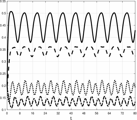
Figure 11: State variables $x_{1}(t)$ [solid line]; $x_{2}(t)$ [dashed line]; $x_{3}(t)$ [dotted line]; and $x_{4}(t)$ [dashdot line] as a function of $t$ in Example 13. Note that each state-variable converges to a periodic function with period $T=8$.

IV-F Rate limiting steps in the RFM and the RFMEO

It has been shown that depending on the biological conditions and the specific organism both initiation and elongation may be rate limiting [56, 8, 69, 40, 53, 60, 22]. Since the RFMEO is a better model for biological translation than the RFM, it is interesting to study the rate limiting step in these two models. We now show that the transition from the low density phase, when initiation is rate limiting, to the high density phase, when elongation is rate limiting is different in the two models: in the RFMEO this transition will take place for a lower initiation rate.

We modeled four S. cerevisiae genes: YMR123W, YNL303W, YJR094W-A, and YBL094C using both an RFMEO with $\ell=10$ and an RFM, and considered the steady-state production rate and the steady-state mean density as a function of the initiation rate $\lambda_{0}$.

As was done in Example 6, the elongation rate $\lambda_{i}$ at each site, for both the RFMEO and the RFM, was estimated using ribo-seq data for the codon decoding rates normalized so that the median elongation rate of all S. cerevisiae mRNAs becomes $6.4$ codons per second. The site rate is simply the corresponding codon rate. These rates thus depend on various factors including availability of tRNA molecules, amino acids, Aminoacyl tRNA synthetase activity and concentration, and local mRNA folding [11, 1, 56].

Fig. 12 depicts the steady-state production rate as a function of $\lambda_{0}$ for the four S. cerevisiae genes for both the RFMEO (upper figure) and the RFM (lower figure). It may be seen that the transition from an initiation rate limiting stage to an elongation rate limiting stage occurs for a lower initiation value in the RFMEO as compared to the RFM.

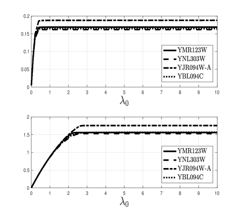
Figure 12: The steady-state production rate $R$ as a function of $\lambda_{0}$ for four S. cerevisiae genes. Upper figure: RFMEO. Lower figure: RFM.

Fig. 13 depicts the steady-state mean density as a function of $\lambda_{0}$ for the four genes and two models. Again, it can be seen that the transition from an initiation rate limiting stage to the elongation rate limiting stage occurs at lower initiations value in the RFMEO as compared to the RFM. This holds for all four genes.

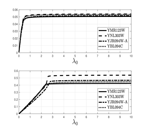
Figure 13: The steady-state mean density $\rho$ as a function of $\lambda_{0}$ for four S. cerevisiae genes. Upper figure: RFMEO. Lower figure: RFM.

V High correlation between RFMEO and TASEPEO

In this section, we show that the RFMEO correlates better with TASEPEO than the RFM, supporting the modeling of intracellular process with multi-site biological machines such as translation and transcription using the RFMEO.

The simulations of TASEPEO with dimension $N$, rates $\mu$ (see (1)), and particle size $\ell$ use a parallel update mode. At each time tick $t_{k}$, the sites along the lattice are scanned from site $N$ backwards to site $1$. If it is time to hop, and the site that is $\ell$ sites in front is empty then the reader advances to the consecutive site. If the site that is $\ell$ sites in front is occupied, the next hopping time, $t_{k}+\varepsilon_{k}$, is generated randomly. For site $i$, $\varepsilon_{k}$ is exponentially distributed with parameter $(1/\mu_{i+1})$ (see (1)). The occupancy at each site is averaged throughout the simulation, with the first $700,000$ cycles discarded in order to obtain the steady-state value. We use $\varrho\in\mathbb{R}^{N}_{+}$ to denote the steady-state reader density, $J:=\beta\varrho_{N}$ to denote the steady-state current (or output rate), and $\sigma:=(1/N)\sum_{i=1}^{N}\varrho_{i}$ for the steady-state mean reader density.

In the examples below, we numerically calculated the Pearson correlation coefficients between the steady-states of the RFMEO, TASEPEO, and RFM.

Example 14

Consider the RFMEO with dimension $n=75$, and transition rates $\lambda_{0}=\cdots=\lambda_{75}=1$. Let $\tilde{e}$ denote the steady-state density of an RFM with the same dimension and rates. We also simulated TASEPEO with dimension $N=75$ and rates $\mu=\lambda$. Fig. 14 depicts the Pearson correlation coefficient $r(e,\varrho)$ between the steady-state reader densities of the RFMEO and the TASEPEO, and the Pearson correlation coefficient $r(\tilde{e},\varrho)$ between the steady-state reader densities of the RFM and TASEPEO, as a function of $\ell\in\{1,\dots,30\}$. The corresponding p-values were all less than $10^{-50}$. It may be seen that $r(e,\varrho)$ and $r(\tilde{e},\varrho)$ are somewhat similar for $\ell\in\{1,\dots,5\}$, however for all $\ell>5$, $r(e,\varrho)>0.94$ whereas $r(\tilde{e},\varrho)$ decreases with $\ell$, and is equal to about $0.825$ for $\ell=30$. Of course, this makes sense as the RFMEO is a mean field approximation of TASEPO. $\square$

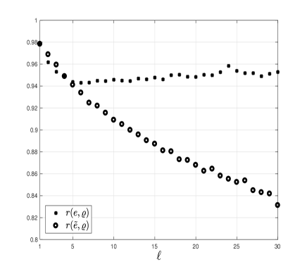
Figure 14: Pearson correlation coefficient $r$ between the steady-state reader densities of the RFMEO ($e$) and TASEPEO ($\varrho$), and between the steady-state reader densities of the RFM ($\tilde{e}$) and TASEPEO ($\varrho$), for $\ell\in\{1,\dots,30\}$.

The following examples consider the case of non-homogeneous transition rates.

Example 15

Consider the RFMEO with dimension $n=40$, particle size $\ell=15$, and rates $\lambda_{i}=1+0.3\sin(2\pi i/41)$, $i=0,\dots,40$. Fig. 15 depicts the RFMEO steady-state reader density $e$, the TASEPEO steady-state reader density $\varrho$ for $\mu=\lambda$, and particle size $15$, and the steady-state density $\tilde{e}$ in the RFM with the same dimension and rates. It can be seen that $e$ provides a far better estimate of $\varrho$ than $\tilde{e}$. $\square$

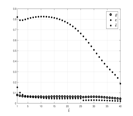
Figure 15: Steady-state density as a function of the site number $i$ for the RFMEO (’+’), TASEPEO (’o’), and RFM (’*’) in Example 15.

In order to verify that the high correlation between RFMEO and TASEPO holds for a large set of parameters, we also simulated the case where the rates are drawn randomly.

Example 16

Consider the RFMEO with dimension $n=100$, particle size $\ell=10$, and rates

$$\lambda_{i}=1+\theta_{i},\quad i=0,\dots,100,$$ (29)

where $\theta_{i}\sim U[-1/2,1/2]$ is a random variable uniformly distributed in the interval $[-1/2,1/2]$. We compared the steady-state production rates of this RFMEO with those of the corresponding TASEPO, and with two RFMs. One RFM with the same dimension and rates. Another RFM, that we refer to as RFM10, is an approximation of the chain with $10$ “codons”/site. Thus, it has dimension $(100/10)-1=9$, where each site contains $10$ consecutive sites of the RFMEO (other than the last site which contains the last $11$ consecutive sites of the RFMEO). The rates of RFM10 are $\gamma_{i}=(\sum_{k=10i}^{T_{i}}\lambda_{k}^{-1})^{-1}$, where $T_{i}=(10(i+1)-1)$ if $i<9$, and otherwise $T_{i}=100$. Note that since the dimension of this RFM$10$ is nine, it cannot be used to estimate the entire density profile of the TASEPEO with dimension $100$.

We ran $300$ tests, where in each test a new set of rates were drawn according to (29). Fig. 16 depicts the correlation between the steady-state production rates of (1) RFMEO and TASEPEO; (2) RFM (i.e. RFM with dimension $100$ and rates $\lambda_{i}$) and TASEPEO, and (3) RFM$10$ and TASEPEO, over the $300$ tests. It may be seen that the RFMEO provides the best correlation with TASEPEO.

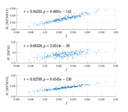
Figure 16: Steady-state production rates, and the corresponding Pearson correlation coefficient $r$ and $p$-value in Example 16. Upper: Steady-state production rates $R$ in RFMEO vs. $J$ in TASEPEO; Middle: Steady-state production rates $R$ in the RFM vs. $J$ in TASEPEO; Lower: Steady-state production rates $R$ in RFM$10$ vs. $J$ in TASEPEO.

Fig. 17 depicts the correlations between the steady-state mean densities for the same three cases. It may be seen that again the correlation between the RFMEO and TASEPEO is high ($r\simeq 0.927$). The correlation between the RFM$10$ and TASEPEO is slightly better ($r\simeq 0.944$), however, as stated above, RFM10 cannot be used to provide an estimate to the actual (per codon) density profile. $\square$

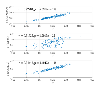
Figure 17: Steady-state mean densities, and the corresponding Pearson correlation coefficient $r$ value and $p$-value in Example 16. Upper: Steady-state mean density $\rho$ in the RFMEO vs. $\sigma$ in TASEPEO; Middle: Steady-state mean density $\rho$ in the RFM vs. $\sigma$ in TASEPEO; Lower: Steady-state mean density $\rho$ in the RFM$10$ vs. $\sigma$ in TASEPEO.

VI Discussion

We studied a deterministic mechanistic model for mRNA translation, the RFMEO, that encapsulates many realistic features of this biological process including the fact that every ribosome covers several codons and that ribosomes cannot overtake one another.

The RFMEO is a mean-field approximation of TASEPEO (see Appendix B) and, as demonstrated above, its simulation results often correlate well with those of TASEPEO. However, unlike TASEPEO, the RFMEO is amenable to rigorous analysis using tools from systems and control theory.

We proved that the RFMEO converges to a unique state-state density and steady-state production rate for any set of feasible transition rates. We follow the terminology used in physics, where an equilibrium point [steady-state] is characterized by a zero [constant but nonzero] total flow of energy [6]. The convergence to this unique steady-state takes place at an exponential rate. In this respect, the RFMEO is robust to the initial conditions.

One may naturally ask whether biological systems are at steady-state (that maybe more general than the steady-state here, e.g. a periodic trajectory). Models with a steady-state (or several of steady-states) have been found to be useful in numerous studies in systems biology (see, e.g. [20] and the references therein). In practice the state of the art routine biological experiments and their interpretation assume steady state as they are performed in a very specific experimental environment which is kept constant during the entire experiment (see, for example, [37, 59, 3]).

In particular, the steady-state in the RFM has been used to accurately predict several features of gene expression (see, e.g., [43, 69, 17]). Here, we used the RFMEO to model a highly-expressed S. cerevisiae gene. The rates were estimated based on biological data. In the resulting RFMEO the convergence to a state close to the steady-state takes approximately 30 seconds, whereas the mRNA half-life is of the order of tens of minutes. This suggests that at least in this case the steady-state assumption is justified.

An important question is how does the steady-state depend on the RFMEO parameters. We proved that increasing any of the RFMEO rates can only increase the steady-state production rate, and that in the totally homogeneous case (i.e. when all the rates are equal) the reader ribosomal density monotonically decreases along the mRNA. In addition, we proved that if one or more of the RFMEO rates are time-varying periodic functions, with a common period $T$, then the densities along the mRNA, and thus also the production rate converge to a periodic solution with period $T$.

The results reported here can shed light on various biophysical aspects of translation, and can be further studied experimentally. For example, our analysis suggests that higher decoding rates at the last $\ell$ codons of the coding region can be expected (since in this region no downstream ribosome can block the ribosome movement). This can be validated experimentally for example based on approaches that track the movement of ribosomes at high resolution [57].

In addition, analysis and simulations of the RFMEO demonstrate several surprising and counterintuitive results. For example, increasing the particle size $\ell$ (i.e. the ribosome footprint) may some times lead to an increase in the production rate. Also, for large $\ell$ the steady-state density along the mRNA may be quite complex (e.g. with quasi-periodic patterns) even for relatively simple (and non-periodic) transition rates. It will be interesting to see if similar patterns are observed experimentally by possibly engineering the codon elongation rates of heterologous or endogenous genes and monitoring translation [57, 21].

We believe that the RFMEO could be useful for modeling, understanding, and re-engineering translation. Specifically, the advantages of the model mentioned above should make it a better candidate than other alternative models for solving some of the open questions in the field [69].

An important topic for future research is using the RFMEO to model ribosome flow based on biological data. This is a challenging task, as many aspects of translation are still not clear. For example, translation initiation is affected by complex phenomena such as the number of free ribosomes, mRNA folding near the 5’end of the mRNA, UTR length and other features, the nucleotide composition surrounding the start codon, and more. In addition, current techniques for measuring ribosome densities provide partial, noisy, and biased data (see, for example, [13]). Thus, using them to estimate the parameters in a computational model like the RFMEO is a non trivial challenge.

Another research topic is using the RFMEO (and networks of RFMEOs) to study various phenomena such as competition for resources in mRNA translation [41, 69], transcription [16], and evolution of transcripts [69].

Appendix A: Proofs

Proof of Prop. 1. Combining (4) and (6) yields

$$\dot{y}_{i}=\sum_{m=1}^{i}\dot{x}_{m}= \lambda_{0}(1-y_{\ell})-\lambda_{i}x_{i}(1-y_{i+\ell}), \quad 1\leq i\leq\ell,$$

$$\dot{y}_{i}=\sum_{\mathclap{m=i-\ell+1}}^{i}\dot{x}_{m}= \lambda_{i-\ell}x_{i-\ell}(1-y_{i})-\lambda_{i}x_{i}(1-y_{i+\ell}), \quad\ell<i\leq n.$$ (30)

By the definition of $y_{i}$, $x_{i}=y_{i}-y_{i-1}+x_{i-\ell},$ and iterating this yields

$$x_{i}=\sum_{k=0}^{\lceil(i-\ell)/\ell\rceil}(y_{i-k\ell}-y_{i-k\ell-1}).$$ (31)

Substituting this in (Appendix A: Proofs) yields (1). ∎

Proof of Prop. 2. Consider the RFMEO with $x(0)\in\partial H$. Then $y(0)=Px(0)$, and there exists an index $i$ such that either $x_{i}(0)\in\{0,1\}$ or $y_{i}(0)\in\{0,1\}$ and all the other entries of $x(0)$ and $y(0)$ are between zero and one. The proof is based on computing the derivatives of the state-variables at time zero, and showing that state-variables that are zero [one] become strictly larger than zero [strictly smaller than one] at time $0^{+}$. We assume throughout that $\ell\geq 2$, as otherwise the RFMEO reduces to the RFM and then the proof follows from the results in [31]. We consider several cases.

Case 1. Suppose that $y_{\ell}(0)=0$. This implies in particular that $x_{\ell}(0)=0$. By (Appendix A: Proofs),

$$\dot{y}_{\ell}(0) =\lambda_{0}(1-y_{\ell}(0))-\lambda_{\ell}x_{\ell}(0)(1-y_{2\ell}(0))$$

$$=\lambda_{0}.$$

Thus, $y_{\ell}(0^{+})>0$. Note that this calculation also implies that for any $\tau>0$ there exists $\varepsilon_{\ell}=\varepsilon_{\ell}(\tau)>0$ such that $y_{\ell}(t,a)\geq\varepsilon_{\ell}$ for all $t\geq\tau$ and all $a\in H$.

Case 2. Suppose that $y_{\ell+1}(0)=0$. This implies in particular that $x_{\ell+1}(0)=0$, so $y_{\ell}(0)=y_{\ell}(0)-y_{\ell+1}(0)=x_{1}(0)-x_{\ell+1}(0)=x_{1}(0)$. By (Appendix A: Proofs),

$$\dot{y}_{\ell+1}(0) =\lambda_{1}x_{1}(0)(1-y_{\ell+1}(0))-\lambda_{\ell+1}x_{\ell+1}(0)(1-y_{2\ell+1}(0))$$

$$=\lambda_{1}y_{\ell}(0).$$

Combining this with the result in Case 1 implies that for any $\tau>0$ there exists $\varepsilon_{\ell+1}=\varepsilon_{\ell+1}(\tau)>0$ such that $y_{\ell+1}(t,a)\geq\varepsilon_{\ell+1}$ for all $t\geq\tau$ and all $a\in H$.

Continuing in this fashion shows that for any $\tau>0$ there exists $\varepsilon=\varepsilon(\tau)>0$ such that $y_{i}(t,a)\geq\varepsilon$ for all $i\in\{\ell,\ell+1,\dots,n\}$, all $t\geq\tau$, and all $a\in H$.

Case 3. Suppose that $x_{j}(0)=0$ for some $j$. Then there exists a minimal index $i$ such that $x_{i}(0)=0$. If $i=n$ then (6) yields

$$\dot{x}_{n}(0) =\lambda_{n-1}x_{n-1}(0)-\lambda_{n}x_{n}(0)$$

$$=\lambda_{n-1}x_{n-1}(0).$$

By the definition of $i$, $x_{n-1}(0)>0$ and thus $x_{n}(0^{+})>0$.

Now suppose that $i=n-1$. Then (6) yields

$$\dot{x}_{n-1}(0) =\lambda_{n-2}x_{n-2}(0)(1-y_{n+\ell-2}(0))-\lambda_{n-1}x_{n-1}(0)$$

$$=\lambda_{n-2}x_{n-2}(0)(1-y_{n+\ell-2}(0)).$$

By the definition of $i$, $x_{n-2}(0)>0$. If $\ell>2$ then $1-y_{n+\ell-2}(0)=1$, and thus $x_{n-1}(0^{+})>0$. If $\ell\leq 2$ then $1-y_{n+\ell-2}(0)=1-y_{n}(0)=1-x_{n}(0)-x_{n-1}(0)=1-x_{n}(0)$. Thus, if $x_{n}(0)<1$ then $x_{n-1}(0^{+})>0$. Consider the case $x_{n}(0)=1$. Then $y_{n}(0)=x_{n-1}(0)+x_{n}(0)=1$, so

$$\dot{y}_{n}(0) =\lambda_{n-\ell}x_{n-\ell}(0)(1-y_{n}(0))-\lambda_{n}x_{n}(0)$$

$$=-\lambda_{n}.$$

This means that $y_{n}(0^{+})<1$, so again we conclude that $x_{n-1}(0^{+})>0$.

Continuing in this fashion shows that if $x_{j}(0)=0$ for some $j$ then $x_{j}(0^{+})>0$. The analysis in all the other relevant cases is very similar, and thus omitted. ∎

Proof of Prop. 3. This follows from the fact that $H$ is compact, convex and with a repelling boundary; see [36, Thm. 2] (see also [32]). ∎

Proof of Prop. 4. Pick $\varepsilon,\tau>0$ and $a,b\in H$. By Prop. 3, there exists $\delta=\delta(\tau)\in(0,1/2)$ such that for all $i$ and all $t\geq\tau$,

$$\delta\leq x_{i}(t),y_{i}(t)\leq 1-\delta.$$ (32)

Write the $q_{j}$s in (6) as

$$q_{j}(x) =\lambda_{j}x_{j}(1-y_{j+\ell})$$

$$=\eta_{j}x_{j}(1-x_{j+1}),$$

where $\eta_{j}(t):=\lambda_{j}\frac{1-y_{j+\ell}(t)}{1-x_{j+1}(t)}.$ Note that (32) implies that

$$0<\lambda_{j}\frac{\delta}{1-\delta}\leq\eta_{j}(t)\leq\lambda_{j}\frac{1-\delta}{\delta}<\infty$$ (33)

for all $j$ and all $t\geq\tau$. Using this notation, the RFMEO in (6) can be written as the time-varying system

$$\dot{x}_{i}=\eta_{j-1}x_{j-1}(1-x_{j})-\eta_{j}x_{j}(1-x_{j+1}).$$

This means that for all $t\geq\tau$ the RFMEO can be interpreted as an RFM with time-varying transition rates $\eta_{j}(t)$ that, by (33), are uniformly bounded and uniformly separated from zero for all $t\geq\tau$. Now the results in [31] imply that there exists $\gamma:=\gamma(\varepsilon)$ such that after time $\tau$ the solutions are contractive with overshoot $(1+\varepsilon)$, and this completes the proof. ∎

Proof of Prop. 5. Consider two RFMEOs, both with the same dimension $n$ and particle size $\ell$. The first with rates $\lambda_{0},\dots,\lambda_{n}$, admits a steady-state density $e$, and a steady-state production rate $R$, and the second with rates $\tilde{\lambda}_{0},\dots,\tilde{\lambda}_{n}$, admits a steady-state density $\tilde{e}$ and a steady-state production rate $\tilde{R}$. Assume that there exists an index $j\in\{0,\dots,n\}$, such that $\tilde{\lambda}_{i}=\lambda_{i}$ for all $i\neq j$, and

$$\tilde{\lambda}_{j}>\lambda_{j}.$$ (34)

We need to show that $\tilde{R}>R$. Seeking a contradiction, assume that

$$\tilde{R}\leq R.$$ (35)

We start with the case $j=n$. Combining (35), (34) and (IV-D) implies that $\tilde{e}_{n}<e_{n}$, and $\tilde{e}_{n-k}\leq e_{n-k}$, $k=1,\dots,\ell-1$. This means that $\tilde{y}_{n}<y_{n}$, and combining this with (35) and (IV-D) implies that $\tilde{e}_{n-\ell}<e_{n-\ell}$, and so $\tilde{y}_{n-1}<y_{n-1}$. Continuing in this way yields $\tilde{e}_{j}<e_{j}$, $j=1,\dots,n-\ell$. In particular, $\tilde{e}_{1}+\dots+\tilde{e}_{\ell}<e_{1}+\dots+e_{\ell}$, and using (IV-D) results in $\tilde{R}>R$. This contradicts (35), and so we conclude that $\tilde{R}>R$ in the case where $\tilde{\lambda}_{n}>\lambda_{n}$.

Using the same approach for any $j\in\{0,\dots,n\}$, while combining the assumption in (35) with (34) and (IV-D), yields

$$\tilde{y}_{k} \leq y_{k},\quad k=j+\ell,\dots,n,$$

$$\tilde{y}_{k} <y_{k},\quad k=\ell,\dots,j+\ell-1.$$ (36)

If $j>0$ then using $k=\ell$ in (Appendix A: Proofs) yields $\tilde{e}_{1}+\dots+\tilde{e}_{\ell}<e_{1}+\dots+e_{\ell}$, thus $\tilde{R}>R$, contradicting (35). If $j=0$ then using $k=\ell$ in (Appendix A: Proofs) yields $\tilde{e}_{1}+\dots+\tilde{e}_{\ell}\leq e_{1}+\dots+e_{\ell}$, but since $\tilde{\lambda}_{0}>\lambda_{0}$, this again yields $\tilde{R}>R$, contradicting (35). We conclude that $\tilde{R}>R$. ∎

Proof of Prop. 6. Consider (IV-D) with $\lambda_{0}=\cdots=\lambda_{n}$. Then

$$e_{n-\ell+1}=\cdots=e_{n}.$$ (37)

Since $e_{n-\ell}(1-e_{n-\ell+1}-\cdots-e_{n})=e_{n-\ell}(1-z_{n})=e_{n-\ell+1}$, and $z_{n}\in(0,1)$, it follows that

$$e_{n-\ell}>e_{n-\ell+1},$$ (38)

and combining this with (37) implies that

$$z_{n-1}>z_{n}.$$ (39)

Now, since $e_{n-\ell-1}(1-e_{n-\ell}-\cdots-e_{n-1})=e_{n-\ell-1}(1-z_{n-1})=e_{n-\ell}(1-z_{n})$, using (39) and the fact that $z_{n-1},z_{n}\in(0,1)$ imply that $e_{n-\ell-1}>e_{n-\ell}$ and thus $z_{n-2}>z_{n-1}$. Continuing in this way completes the proof. ∎

Proof of Prop. 7. Let $e$ $[\bar{e}]$ denote the steady-state reader density in the RFMEO [RFM]. We need to show that $\bar{R}>R$. Seeking a contradiction, assume that

$$\bar{R}\leq R.$$ (40)

Combining this with (IV-D) for both the RFMEO with particle size $\ell$ and with particle size one (i.e. the RFM), it follows that $\lambda_{0}(1-\bar{e}_{1})\leq\lambda_{0}(1-e_{1}-\dots-e_{\ell})$, thus

$$\bar{e}_{1}\geq e_{1}+\dots+e_{\ell},$$

and since $e\in\operatorname{{\mathrm{i}nt}}(H)$ this yields

$$\bar{e}_{1}>e_{1}.$$ (41)

Using (IV-D), (40), and (41), it follows that

$$\bar{e}_{2}>e_{2}+\dots+e_{\ell+1},$$

and since $e\in\operatorname{{\mathrm{i}nt}}(H)$ this yields

$$\bar{e}_{2}>e_{2}.$$

Continuing in this way yields

$$\bar{e}_{j}>e_{j}+\dots+e_{j+\ell-1},\quad j=2,\dots,n-\ell+1,$$ (42)

so in particular,

$$\bar{e}_{n-\ell+1}>e_{n-\ell+1}+\dots+e_{n}.$$ (43)

On the other-hand using (40) and comparing the last $\ell$ equations in (IV-D) for both the RFMEO with particle size $\ell$ and with particle size one (i.e. the RFM), yields

$$\bar{e}_{n-\ell+1}(1-\bar{e}_{n-\ell+2}) \leq e_{n-\ell+1},$$

$$\bar{e}_{n-\ell+2}(1-\bar{e}_{n-\ell+3}) \leq e_{n-\ell+2},$$

$$\dots$$

$$\bar{e}_{n-1}(1-\bar{e}_{n}) \leq e_{n-1},$$

$$\bar{e}_{n} \leq e_{n}.$$ (44)

Now combining (Appendix A: Proofs) with (43) yields

$$\bar{e}_{n-\ell+2}(1-\bar{e}_{n-\ell+1})+\bar{e}_{n-\ell+3}(1-\bar{e}_{n-\ell+2})+\dots+\bar{e}_{n}(1-\bar{e}_{n-1})<0.$$ (45)

However, since $\bar{e}\in\operatorname{{\mathrm{i}nt}}(H)$, the term on the left-hand side here must be strictly positive. This contradiction completes the proof. ∎

Appendix B: RFMEO as a Mean-Field Approximation of TASEPEO

In this appendix, we show how the RFMEO can be derived from TASEPEO. We use a notation that is standard in the TASEPEO literature.

Consider TASEPEO with $N$ sites, rates $\mu$ defined in (1), extended object size $\ell$, and under the assumption that the reader is located at the left-most site of the object. Following MacDonald et. al. [29] (see also [30]) the current from site $i$ to site $i+1$ at time $t$ is given by (for simplicity we ignore boundary cases):

$$J_{i\to i+1}(t) =\gamma_{i}\operatorname{Pr}(\text{site }i\text{ has a reader and site }i+\ell\text{ is empty})$$

$$=\gamma_{i}\operatorname{Pr}(\text{site }i\text{ has a reader})\operatorname{Pr}(\text{site }i+\ell\text{ is empty }|\text{ site }i\text{ has a reader}),$$ (46)

where $\operatorname{Pr}(a)$ [$\operatorname{Pr}(a|b)$] denotes the probability of event $a$ [the conditional probability of event $a$ given event $b$] at time $t$. Since the conditional probability in (Appendix B: RFMEO as a Mean-Field Approximation of TASEPEO) is difficult to estimate, we apply what [14] calls a naive mean-field approximation, and replace (Appendix B: RFMEO as a Mean-Field Approximation of TASEPEO) by:

$$J_{i\to i+1}(t) =\gamma_{i}\operatorname{Pr}(\text{site }i\text{ has a reader})\operatorname{Pr}(\text{site }i+\ell\text{ is empty})$$

$$=\gamma_{i}\operatorname{Pr}(\text{site }i\text{ has a reader})\left(1-\sum_{k=0}^{\ell-1}\operatorname{Pr}(\text{site }i+\ell-k\text{ has a reader})\right).$$ (47)

We approximate the probabilities above by averaging the binary reader occupancies over an ensemble of TASEPEO systems, i.e. we replace $\operatorname{Pr}(\text{site }i\text{ has a reader})$ by $\rho^{r}_{i}(t):=\langle r_{i}(t)\rangle$, where $r_{i}(t)\in\{0,1\}$ is the reader occupancy at site $i$ at time $t$, and the operator $\langle\rangle$ denotes an average over the ensemble. This yields

$$J_{i\to i+1}(t)=\gamma_{i}\rho^{r}_{i}(t)\left(1-\sum_{k=0}^{\ell-1}\rho^{r}_{i+\ell-k}(t)\right).$$ (48)

The change in the average reader occupancy at site $i$ at time $t$ is given by [29]:

$$\frac{d}{dt}\rho^{r}_{i}(t)=J_{i-1\to i}(t)-J_{i\to i+1}(t).$$ (49)

Introducing the notation $x_{i}(t):=\rho^{r}_{i}(t)$ and $\lambda_{i}:=\gamma_{i},$ we see that $J_{i\to i+1}(t)$ corresponds to $q_{i}(x)$ in (7), and (49) corresponds to (6) (see (4)). Thus, we obtained the RFMEO. In particular, the case $\ell=1$ in (48) corresponds to the dynamical equations of the RFM (see (3)).

At steady-state, we expect every $\rho^{r}_{i}(t)$ in TASEPEO to converge to, say, $\rho^{r}_{i}$, and then the currents between any two consecutive sites are all equal (but we are not aware of any rigorous proof of convergence in TASEPEO). The derivation above (including the boundary cases as well [30, 14]) shows that the steady-state current satisfies:

$$J =\alpha(1-\sum_{k=0}^{\ell-1}\rho^{r}_{\ell-k})$$

$$=\gamma_{i}\rho^{r}_{i}(1-\sum_{k=0}^{\ell-1}\rho^{r}_{i+\ell-k}) 1\leq i\leq N-\ell$$ for all

$$=\gamma_{i}\rho^{r}_{i} N-\ell+1\leq i\leq N-1$$ for all

$$=\beta\rho^{r}_{N}.$$ (50)

If we use the notation $e_{i}:=\rho^{r}_{i}$, $\lambda_{0}:=\alpha$, and $\lambda_{n}:=\beta$ then this is just the steady-state equation of RFMEO given in (IV-D).

References

- [1] B. Alberts, A. Johnson, J. Lewis, M. Raff, K. Roberts, and P. Walter, Molecular Biology of the Cell. New York: Garland Science, 2008.
- [2] Z. Aminzare and E. D. Sontag, “Contraction methods for nonlinear systems: A brief introduction and some open problems,” in Proc. 53rd IEEE Conf. on Decision and Control, Los Angeles, CA, 2014, pp. 3835–3847.
- [3] Z. Bar-Joseph, A. Gitter, and S. I., “Studying and modelling dynamic biological processes using time-series gene expression data,” Nat. Rev. Genet., vol. 13, no. 8, pp. 552–64, 2012.
- [4] R. A. Blythe and M. R. Evans, “Nonequilibrium steady states of matrix-product form: a solver’s guide,” J. Phys. A: Math. Gen., vol. 40, no. 46, pp. R333–R441, 2007.
- [5] C. A. Brackley, D. S. Broomhead, M. C. Romano, and M. Thiel, “A max-plus model of ribosome dynamics during mRNA translation,” J. Theoretical Biology, vol. 303, pp. 128–140, 2012.
- [6] A. C. Burton, “The properties of the steady state compared to those of equilibrium as shown in characteristic biological behavior,” J. Cellular and Comparative Physiology, vol. 14, no. 3, pp. 327–349, 1939.
- [7] D. Chu, N. Zabet, and T. von der Haar, “A novel and versatile computational tool to model translation,” Bioinformatics, vol. 28, no. 2, pp. 292–3, 2012.
- [8] L. Ciandrini, I. Stansfield, and M. Romano, “Ribosome traffic on mRNAs maps to gene ontology: genome-wide quantification of translation initiation rates and polysome size regulation,” PLOS Computational Biology, vol. 9, p. e1002866, 2013.
- [9] A. Dana and T. Tuller, “Determinants of translation elongation speed and ribosomal profiling biases in mouse embryonic stem cells,” PLOS Computational Biology, vol. 8, no. 12, p. e1002755, 2012.
- [10] A. Dana and T. Tuller, “Efficient manipulations of synonymous mutations for controlling translation rate–an analytical approach,” J. Comput. Biol., vol. 19, pp. 200–231, 2012.
- [11] A. Dana and T. Tuller, “Mean of the typical decoding rates: a new translation efficiency index based on the analysis of ribosome profiling data,” G3, vol. 5, no. 1, pp. 73–80, 2014.
- [12] C. Deneke, R. Lipowsky, and A. Valleriani, “Effect of ribosome shielding on mRNA stability,” Phys. Biol., vol. 10, no. 4, p. 046008, 2013.
- [13] A. Diament and T. Tuller, “Estimation of ribosome profiling performance and reproducibility at various levels of resolution,” Biol. Direct., vol. 11, no. 24, 2016.
- [14] J. J. Dong, B. Schmittmann, and R. K. P. Zia, “Inhomogeneous exclusion processes with extended objects: The effect of defect locations,” Phys. Rev. E, vol. 76, p. 051113, 2007.
- [15] J. J. Dong, R. K. P. Zia, and B. Schmittmann, “Understanding the edge effect in TASEP with mean-field theoretic approaches,” J. Phys. A: Math. Gen., vol. 42, no. 1, p. 015002, 2008.
- [16] S. Edri, E. Gazit, E. Cohen, and T. Tuller, “The RNA polymerase flow model of gene transcription,” IEEE Trans. Biomed. Circuits Syst., vol. 8, no. 1, pp. 54–64, 2014.
- [17] S. Edri and T. Tuller, “Quantifying the effect of ribosomal density on mRNA stability,” PLoS One, vol. 9, no. 7, p. e102308, 2014.
- [18] E. Eisenberg and E. Y. Levanon, “Human housekeeping genes are compact,” Trends Genet., vol. 19, no. 7, pp. 362–5, 2003.
- [19] H. Ez-Zahraouy, K. Jetto, and A. Benyoussef, “The effect of mixture lengths of vehicles on the traffic flow behaviour in one-dimensional cellular automaton,” The European Physical Journal B-Condensed Matter and Complex Systems, vol. 40, no. 1, pp. 111–117, 2004.
- [20] J. Gunawardena, “Models in systems biology: The parameter problem and the meanings of robustness,” in Elements of Computational Systems Biology, H. M. Lodhi and S. H. Muggleton, Eds. Wiley, 2010, pp. 21–48.
- [21] N. T. Ingolia, S. Ghaemmaghami, J. R. Newman, and J. S. Weissman, “Genome-wide analysis in vivo of translation with nucleotide resolution using ribosome profiling,” Science, vol. 324, no. 5924, pp. 218–23, 2009.
- [22] N. Jacques and M. Dreyfus, “Translation initiation in Escherichia coli: old and new questions,” Mol Microbiol., vol. 4, no. 7, pp. 1063–7, 1990.
- [23] M. Kaczanowska and M. Ryden-Aulin, “Ribosome biogenesis and the translation process in Escherichia coli,” Microbiol Mol Biol Rev, vol. 71, p. 477 494, 2007.
- [24] T. V. Karpinets, D. J. Greenwood, C. E. Sams, and J. T. Ammons, “RNA: protein ratio of the unicellular organism as a characteristic of phosphorous and nitrogen stoichiometry and of the cellular requirement of ribosomes for protein synthesis,” BMC Biol., vol. 4, no. 30, pp. 274–80, 2006.
- [25] B. S. Kerner, “The physics of green-wave breakdown in a city,” Europhysics Letters, vol. 102, no. 2, p. 28010, 2013.
- [26] S. Kuhner, V. van Noort, M. Betts, A. Leo-Macias, C. Batisse, M. Rode, T. Yamada, T. Maier, S. Bader, P. Beltran-Alvarez, D. Casta o-Diez, W. Chen, D. Devos, M. Guell, T. Norambuena, I. Racke, V. Rybin, A. Schmidt, E. Yus, R. Aebersold, R. Herrmann, B. B ttcher, A. Frangakis, R. Russell, P. Serrano, L. Bork, and A. Gavin, “Proteome organization in a genome-reduced bacterium,” Science, vol. 326, no. 5957, pp. 1235–40, 2009.
- [27] G. Lakatos and T. Chou, “Totally asymmetric exclusion processes with particles of arbitrary size,” J. Phys. A: Math. Gen., vol. 36, p. 20272041, 2003.
- [28] W. Lohmiller and J.-J. E. Slotine, “On contraction analysis for non-linear systems,” Automatica, vol. 34, pp. 683–696, 1998.
- [29] C. T. MacDonald, J. H. Gibbs, and A. C. Pipkin, “Kinetics of biopolymerization on nucleic acid templates,” Biopolymers, vol. 6, pp. 1–25, 1968.
- [30] C. T. MacDonald and J. H. Gibbs, “Concerning the kinetics of polypeptide synthesis on polyribosomes,” Biopolymers, vol. 7, no. 5, pp. 707–725, 1969.
- [31] M. Margaliot, E. D. Sontag, and T. Tuller, “Entrainment to periodic initiation and transition rates in a computational model for gene translation,” PLoS ONE, vol. 9, no. 5, p. e96039, 2014.
- [32] M. Margaliot, E. D. Sontag, and T. Tuller, “Contraction after small transients,” Automatica, vol. 67, pp. 178–184, 2016.
- [33] M. Margaliot and T. Tuller, “On the steady-state distribution in the homogeneous ribosome flow model,” IEEE/ACM Trans. Computational Biology and Bioinformatics, vol. 9, pp. 1724–1736, 2012.
- [34] M. Margaliot and T. Tuller, “Stability analysis of the ribosome flow model,” IEEE/ACM Trans. Computational Biology and Bioinformatics, vol. 9, pp. 1545–1552, 2012.
- [35] M. Margaliot and T. Tuller, “Ribosome flow model with positive feedback,” J. Royal Society Interface, vol. 10, p. 20130267, 2013.
- [36] M. Margaliot, T. Tuller, and E. D. Sontag, “Checkable conditions for contraction after small transients in time and amplitude,” in Feedback Stabilization of Controlled Dynamical Systems: In Honor of Laurent Praly, N. Petit, Ed. Cham: Springer International Publishing, 2017, pp. 279–305.
- [37] S. Mukherji, M. Ebert, G. Zheng, J. Tsang, P. Sharp, and A. van Oudenaarden, “MicroRNAs can generate thresholds in target gene expression,” Nat. Genet., vol. 43, no. 9, pp. 854–9, 2011.
- [38] G. Poker, Y. Zarai, M. Margaliot, and T. Tuller, “Maximizing protein translation rate in the nonhomogeneous ribosome flow model: a convex optimization approach,” J. Royal Society Interface, vol. 11, no. 100, 2014.
- [39] G. Poker, M. Margaliot, and T. Tuller, “Sensitivity of mRNA translation,” Sci. Rep., vol. 5, p. 12795, 2015.
- [40] J. Racle, F. Picard, L. Girbal, M. Cocaign-Bousquet, and V. Hatzimanikatis, “A genome-scale integration and analysis of Lactococcus lactis translation data,” PLOS Computational Biology, vol. 9, p. e1003240, 2013.
- [41] A. Raveh, M. Margaliot, E. Sontag, and T. Tuller, “A model for competition for ribosomes in the cell,” J. Royal Society Interface, vol. 13, no. 116, p. 20151062, 2016.
- [42] A. Raveh, Y. Zarai, M. Margaliot, and T. Tuller, “Ribosome flow model on a ring,” IEEE/ACM Trans. Computational Biology and Bioinformatics, vol. 12, no. 6, pp. 1429–1439, 2015.
- [43] S. Reuveni, I. Meilijson, M. Kupiec, E. Ruppin, and T. Tuller, “Genome-scale analysis of translation elongation with a ribosome flow model,” PLOS Computational Biology, vol. 7, p. e1002127, 2011.
- [44] G. Rice, M. Chamberlin, and C. Kane, “Contacts between mammalian RNA polymerase II and the template DNA in a ternary elongation complex,” Nucleic Acids Res., vol. 21, no. 1, pp. 113–8, 1993.
- [45] G. Russo, M. di Bernardo, and E. D. Sontag, “Global entrainment of transcriptional systems to periodic inputs,” PLOS Computational Biology, vol. 6, p. e1000739, 2010.
- [46] A. Schadschneider, D. Chowdhury, and K. Nishinari, Stochastic Transport in Complex Systems: From Molecules to Vehicles. Elsevier, 2011.
- [47] P. Shah, Y. Ding, M. Niemczyk, G. Kudla, and J. Plotkin, “Rate-limiting steps in yeast protein translation,” Cell, vol. 153, no. 7, pp. 1589–601, 2013.
- [48] O. Shalem, O. Dahan, M. Levo, M. Martinez, I. Furman, E. Segal, and P. Y., “Transient transcriptional responses to stress are generated by opposing effects of mrna production and degradation,” Mol Syst Biol., vol. 4, p. 223, 2008.
- [49] L. B. Shaw, R. K. P. Zia, and K. H. Lee, “Totally asymmetric exclusion process with extended objects: a model for protein synthesis,” Phys. Rev. E, vol. 68, p. 021910, 2003.
- [50] L. B. Shaw, A. B. Kolomeisky, and K. H. Lee, “Local inhomogeneity in asymmetric simple exclusion processes with extended objects,” Journal of Physics A: Mathematical and General, vol. 37, no. 6, p. 2105, 2004.
- [51] L. B. Shaw, J. P. Sethna, and K. H. Lee, “Mean-field approaches to the totally asymmetric exclusion process with quenched disorder and large particles,” Phys. Rev. E, vol. 70, no. 2, p. 021901, 2004.
- [52] H. L. Smith, Monotone Dynamical Systems: An Introduction to the Theory of Competitive and Cooperative Systems, ser. Mathematical Surveys and Monographs. Providence, RI: Amer. Math. Soc., 1995, vol. 41.
- [53] T. Tuller, A. Carmi, K. Vestsigian, S. Navon, Y. Dorfan, J. Zaborske, T. Pan, O. Dahan, I. Furman, and Y. Pilpel, “An evolutionarily conserved mechanism for controlling the efficiency of protein translation,” Cell, vol. 141, no. 2, pp. 344–54, 2010.
- [54] T. Tuller, M. Kupiec, and E. Ruppin, “Determinants of protein abundance and translation efficiency in S. cerevisiae.” PLOS Computational Biology, vol. 3, pp. 2510–2519, 2007.
- [55] T. Tuller, I. Veksler, N. Gazit, M. Kupiec, E. Ruppin, and M. Ziv, “Composite effects of gene determinants on the translation speed and density of ribosomes,” Genome Biol., vol. 12, no. 11, p. R110, 2011.
- [56] T. Tuller and H. Zur, “Multiple roles of the coding sequence 5’ end in gene expression regulation,” Nucleic Acids Res., vol. 43, no. 1, pp. 13–28, 2015.
- [57] S. Uemura, C. E. Aitken, J. Korlach, B. A. Flusberg, S. W. Turner, and J. D. Puglisi, “Real-time tRNA transit on single translating ribosomes at codon resolution,” Nature, vol. 464, pp. 1012–1017, 2010.
- [58] A. Verschoor, J. R. Warner, S. Srivastava, R. A. Grassucci, and J. Frank, “Three-dimensional structure of the yeast ribosome,” Nucleic Acids Res., vol. 26, no. 2, pp. 655–61, 1998.
- [59] C. Vogel and E. Marcotte, “Insights into the regulation of protein abundance from proteomic and transcriptomic analyses,” Nat. Rev. Genet., vol. 13, no. 4, pp. 227–32, 2012.
- [60] T. von der Haar, “Mathematical and computational modelling of ribosomal movement and protein synthesis: an overview,” Comput. Struct. Biotechnol. J., vol. 1, p. e201204002, 2012.
- [61] Y. Wang, C. Liu, J. Storey, R. Tibshirani, D. Herschlag, and P. Brown, “Precision and functional specificity in mRNA decay,” Proceedings of the National Academy of Sciences, vol. 99, no. 9, pp. 5860–5, 2002.
- [62] Y. Zarai, M. Margaliot, E. D. Sontag, and T. Tuller, “Controllability analysis and control synthesis for the ribosome flow model,” IEEE/ACM Trans. Computational Biology and Bioinformatics, 2017, to appear. [Online]. Available: http://arxiv.org/abs/1602.02308
- [63] Y. Zarai, M. Margaliot, and T. Tuller, “Explicit expression for the steady-state translation rate in the infinite-dimensional homogeneous ribosome flow model,” IEEE/ACM Trans. Computational Biology and Bioinformatics, vol. 10, pp. 1322–1328, 2013.
- [64] Y. Zarai, M. Margaliot, and T. Tuller, “Optimal down regulation of mRNA translation,” Sci. Rep., vol. 7, no. 41243, 2017.
- [65] Y. Zarai, M. Margaliot, and T. Tuller, “On the ribosomal density that maximizes protein translation rate,” PLOS ONE, vol. 11, no. 11, pp. 1–26, 11 2016.
- [66] G. Zhang and Z. Ignatova, “Folding at the birth of the nascent chain: coordinating translation with co-translational folding,” Curr Opin Struct Biol., no. 1, pp. 25–31, 2011.
- [67] Y.-B. Zhao and J. Krishnan, “mRNA translation and protein synthesis: an analysis of different modelling methodologies and a new PBN based approach,” BMC Systems Biology, vol. 8, no. 1, p. 25, 2014.
- [68] R. K. P. Zia, J. Dong, and B. Schmittmann, “Modeling translation in protein synthesis with TASEP: A tutorial and recent developments,” J. Statistical Physics, vol. 144, pp. 405–428, 2011.
- [69] H. Zur and T. Tuller, “Predictive biophysical modeling and understanding of the dynamics of mRNA translation and its evolution,” Nucleic Acids Res., vol. 44, no. 19, pp. 9031–9049, 2016.