On the number of types in sparse graphs

Abstract

We prove that for every class of graphs $\mathcal{C}$ which is nowhere dense, as defined by Nešetřil and Ossona de Mendez [27, 28], and for every first order formula $\varphi(\bar{x},\bar{y})$, whenever one draws a graph $G\in\mathcal{C}$ and a subset of its nodes $A$, the number of subsets of $A^{|\bar{y}|}$ which are of the form $\{\bar{v}\in A^{|\bar{y}|}\,\colon\,G\models\varphi(\bar{u},\bar{v})\}$ for some valuation $\bar{u}$ of $\bar{x}$ in $G$ is bounded by $\mathcal{O}(|A|^{|\bar{x}|+\varepsilon})$, for every $\varepsilon>0$. This provides optimal bounds on the VC-density of first-order definable set systems in nowhere dense graph classes.

We also give two new proofs of upper bounds on quantities in nowhere dense classes which are relevant for their logical treatment. Firstly, we provide a new proof of the fact that nowhere dense classes are uniformly quasi-wide, implying explicit, polynomial upper bounds on the functions relating the two notions. Secondly, we give a new combinatorial proof of the result of Adler and Adler [1] stating that every nowhere dense class of graphs is stable. In contrast to the previous proofs of the above results, our proofs are completely finitistic and constructive, and yield explicit and computable upper bounds on quantities related to uniform quasi-wideness (margins) and stability (ladder indices).

1 Introduction

Nowhere dense classes of graphs were introduced by Nešetřil and Ossona de Mendez [27, 28] as a general and abstract model capturing uniform sparseness of graphs. These classes generalize many familiar classes of sparse graphs, such as planar graphs, graphs of bounded treewidth, graphs of bounded degree, and, in fact, all classes that exclude a fixed topological minor. Formally, a class $\mathcal{C}$ of graphs is nowhere dense if there is a function $t\colon\mathbb{N}\to\mathbb{N}$ such that for every $r\in\mathbb{N}$, no graph $G$ in $\mathcal{C}$ contains the clique $K_{t(r)}$ on $t(r)$ vertices as depth-$r$ minor, i.e., as a subgraph of a graph obtained from $G$ by contracting mutually disjoint subgraphs of radius at most $r$ to single vertices. The more restricted notion of bounded expansion requires in addition that for every fixed $r$, there is a constant (depending on $r$) upper bound on the ratio between the number of edges and the number of vertices in depth-$r$ minors of graphs from $\mathcal{C}$.

The concept of nowhere denseness turns out to be very robust, as witnessed by the fact that it admits multiple different characterizations, uncovering intricate connections to seemingly distant branches of mathematics. For instance, nowhere dense graph classes can be characterized by upper bounds on the density of bounded-depth (topological) minors [27, 28], by uniform quasi-wideness [28] (a notion introduced by Dawar [9] in the context of homomorphism preservation properties), by low tree-depth colorings [26], by generalized coloring numbers [37], by sparse neighborhood covers [17, 18], by a game called the splitter game [18], and by the model-theoretic concepts of stability and independence [1]. For a broader discussion on graph theoretic sparsity we refer to the book of Nešetřil and Ossona de Mendez [29].

The combination of combinatorial and logical methods yields a powerful toolbox for the study of nowhere dense graph classes. In particular, the result of Grohe, Kreutzer and the second author [18] exploits this combination in order to prove that a given first order sentence $\varphi$ can be evaluated in time $f(\varphi)\cdot n^{1+\varepsilon}$ on $n$-vertex graphs from a fixed nowhere dense class of graphs $\mathcal{C}$, for any fixed real $\varepsilon>0$ and some function $f$. On the other hand, provided $\mathcal{C}$ is closed under taking subgraphs, it is known that if $\mathcal{C}$ is not nowhere dense, then there is no algorithm with running time of the form $f(\varphi)\cdot n^{c}$ for any constant $c$ under plausible complexity assumptions [12]. In the terminology of parameterized complexity, these results show that the notion of nowhere denseness exactly characterized subgraph-closed classes where model-checking first order logic is fixed-parameter tractable, and conclude a long line of research concerning the parameterized complexity of the model checking problem for sparse graph classes (see [16] for a survey).

Summary of contribution.

In this paper, we continue the study of the interplay of combinatorial and logical properties of nowhere dense graph classes, and provide new upper bounds on several quantities appearing in their logical study. Our main focus is on the notion of VC-density for first order formulas. This concept originates from model theory and aims to measure the complexity of set systems definable by first order formulas, similarly to the better-known VC-dimension. We give optimal bounds on the VC-density in nowhere dense graph classes, and in particular we show that these bounds are “as good as one could hope for”.

We also provide new upper bounds on quantities related to stability and uniform quasi-wideness of nowhere dense classes. For stability, we provide explicit and computable upper bounds on the ladder index of any first order formula on a given nowhere dense class. For uniform quasi-wideness, we give a new, purely combinatorial proof of polynomial upper bounds on margins, that is, functions governing this notion. We remark that the existence of upper bounds as above is known [1, 21], but the proofs are based on nonconstructive arguments, notably the compactness theorem for first order logic. Therefore, the upper bounds are given purely existentially and are not effectively computable. Contrary to these, our proofs are entirely combinatorial and effective, yielding computable upper bounds.

We now discuss the relevant background from logic and model theory, in order to motivate and state our results.

Model theory.

Our work is inspired by ideas from model theory, more specifically, from stability theory. The goal of stability theory is to draw certain dividing lines specifying abstract properties of logical structures which allow the development of a good structure theory. There are many such dividing lines, depending on the specifics of the desired theory. One such dividing line encloses the class of stable structures, another encloses the larger class of dependent structures (also called NIP). A general theme is that the existence of a manageable structure is strongly related to the non-existence of certain forbidden patterns on one hand, and on the other hand, to bounds on cardinalities of certain type sets. Let us illustrate this phenomenon more concretely.

For a first order formula $\varphi(\bar{x},\bar{y})$ with free variables split into $\bar{x}$ and $\bar{y}$, a $\varphi$-ladder of length $n$ in a logical structure $\mathbb{A}$ is a sequence $\bar{u}_{1},\ldots,\bar{u}_{n},\bar{v}_{1},\ldots,\bar{v}_{n}$ of tuples of elements of $\mathbb{A}$ such that

$$\mathbb{A}\models\varphi(\bar{u}_{i},\bar{v}_{j})\ \Longleftrightarrow\ i\leqslant j\qquad\text{for all $1\leqslant i,j\leqslant n$.}$$

The least $n$ for which there is no $\varphi$-ladder of length $n$ is the ladder index of $\varphi(\bar{x},\bar{y})$ in $\mathbb{A}$ (which may depend on the split of the variables, and may be $\infty$ for some infinite structures $\mathbb{A}$). A class of structures $\mathcal{C}$ is stable if the ladder index of every first order formula $\varphi(\bar{x},\bar{y})$ over structures from $\mathcal{C}$ is bounded by a constant depending only on $\varphi$ and $\mathcal{C}$. This notion can be applied to a single infinite structure $\mathbb{A}$, by considering the class consisting of $\mathbb{A}$ only. Examples of stable structures include $(\mathbb{N},=)$, the field of complex numbers $(\mathbb{C},+,\times,0,1)$, as well as any vector space $V$ over the field of rationals, treated as a group with addition. On the other hand, $(\mathbb{Q},\leqslant)$ and the field of reals $(\mathbb{R},+,\times,0,1)$ are not stable, as they admit a linear ordering which is definable by a first order formula. Stable structures turn out to have more graspable structure than unstable ones, as they can be equipped with various notions useful for their study, such as forking independence (generalizing linear independence in vector spaces) and rank (generalizing dimension). We refer to the textbooks [30, 36] for an introduction to stability theory.

One of concepts studied in the early years of stability theory is a property of infinite graphs called superflatness, introduced by Podewski and Ziegler [31]. The definition of superflatness is the same as of nowhere denseness, but Podewski and Ziegler, instead of applying it to an infinite class of finite graphs, apply it to a single infinite graph. The main result of [31] is that every superflat graph is stable. As observed by Adler and Adler [1], this directly implies the following:

Theorem 1 ([1, 31]).

Every nowhere dense class of graphs is stable. Conversely, any stable class of finite graphs which is subgraph-closed is nowhere dense.

Thus, the notion of nowhere denseness (or superflatness) coincides with stability if we restrict attention to subgraph-closed graph classes.

The proof of Adler and Adler does not yield effective or computable upper bound on the ladder index of a given formula for a given nowhere dense class of graphs, as it relies on the result of Podewski and Ziegler, which in turn invokes compactness for first order logic.

Cardinality bounds.

One of the key insights provided by the work of Shelah is that stable classes can be characterized by admitting strong upper bounds on the cardinality of Stone spaces. For a first order formula $\varphi(\bar{x},\bar{y})$ with free variables partitioned into object variables $\bar{x}$ and parameter variables $\bar{y}$, a logical structure $\mathbb{A}$, and a subset of its domain $B$, define the set of $\varphi$-types with parameters from $B$, which are realized in $\mathbb{A}$, as follows:

$$S^{\varphi}(\mathbb{A}/B)=\left\{\big{\{}\bar{v}\ \in B^{|\bar{y}|}\,\colon\,\mathbb{A}\models\varphi(\bar{u},\bar{v})\big{\}}\colon\,\bar{u}\in V(\mathbb{A})^{|\bar{x}|}\right\}\ \subseteq\ \mathcal{P}(B^{|\bar{y}|}).$$ (1)

Here, $V(\mathbb{A})$ denotes the domain of $\mathbb{A}$ and $\mathcal{P}(X)$ denotes the powerset of $X$. Putting the above definition in words, every tuple $\bar{u}\in V(\mathbb{A})^{|\bar{x}|}$ defines the set of those tuples $\bar{v}\in B^{|\bar{y}|}$ for which $\varphi(\bar{u},\bar{v})$ holds. The set $S^{\varphi}(\mathbb{A}/B)$ consists of all subsets of $B^{|\bar{y}|}$ that can be defined in this way.

Note that in principle, $S^{\varphi}(\mathbb{A}/B)$ may be equal to $\mathcal{P}(B^{|\bar{x}|})$, and therefore have very large cardinality compared to $B$, even for very simple formulas. The following characterization due to Shelah (cf. [35, Theorem 2.2, Chapter II]) shows that for stable classes this does not happen.

Theorem 2.

A class of structures $\cal C$ is stable if and only if there is an infinite cardinal $\kappa$ such that the following holds for all structures $\mathbb{A}$ in the elementary closure of $\cal C$, and all $B\subseteq V(\mathbb{A})$:

$$\textit{if\quad}|B|\leqslant\kappa\textit{\quad then\quad}|S^{\varphi}(\mathbb{A}/B)|\leqslant\kappa.$$

Therefore, Shelah’s result provides an upper bound on the number of types, albeit using infinite cardinals, elementary limits, and infinite parameter sets. The cardinality bound provided by theorem 2, however, does not seem to immediately translate to a result of finitary nature. As we describe below, this can be done using the notions of VC-dimension and VC-density.

VC-dimension and VC-density.

The notion of VC-dimension was introduced by Vapnik and Chervonenkis [8] as a measure of complexity of set systems, or equivalently of hypergraphs. Over the years it has found important applications in many areas of statistics, discrete and computational geometry, and learning theory.

Formally, VC-dimension is defined as follows. Let $X$ be a set and let $\mathcal{F}\subseteq\mathcal{P}(X)$ be a family of subsets of $X$. A subset $A\subseteq X$ is shattered by $\mathcal{F}$ if $\{A\cap F\colon F\in\mathcal{F}\}=\mathcal{P}(A)$; that is, every subset of $A$ can be obtained as the intersection of some set from $\mathcal{F}$ with $A$. The VC-dimension, of $\mathcal{F}$ is the maximum size of a subset $A\subseteq X$ that is shattered by $\mathcal{F}$.

As observed by Laskowski [22], VC-dimension can be connected to concepts from stability theory introduced by Shelah. For a given structure $\mathbb{A}$, parameter set $B\subseteq V(\mathbb{A})$, and formula $\varphi(\bar{x},\bar{y})$, we may consider the family $S^{\varphi}(\mathbb{A}/B)$ of subsets of $B^{|\bar{y}|}$ defined using equation (1). The VC-dimension of $\varphi(\bar{x},\bar{y})$ on $\mathbb{A}$ is the VC-dimension of the family $S^{\varphi}(\mathbb{A}/V(\mathbb{A}))$. In other words, the VC-dimension of $\varphi(\bar{x},\bar{y})$ on $\mathbb{A}$ is the largest cardinality of a finite set $I$ for which there exist families of tuples $(\bar{u}_{i})_{i\in I}$ and $(\bar{v}_{J})_{J\subseteq I}$ of elements of $\mathbb{A}$ such that

$$\mathbb{A}\models\varphi(\bar{u}_{i},\bar{v}_{J})\Longleftrightarrow i\in J\qquad\text{for all $i\in I$ and $J\subseteq I$.}$$

A formula $\varphi(\bar{x},\bar{y})$ is dependent on a class of structures $\cal C$ if there is a bound $d\in\mathbb{N}$ such that the VC-dimension of $\varphi(\bar{x},\bar{y})$ on $\mathbb{A}$ is at most $d$ for all $\mathbb{A}\in\cal C$. It is immediate from the definitions that if a formula $\varphi(\bar{x},\bar{y})$ is stable over $\cal C$, then it is also dependent on $\cal C$ (the bound being the ladder index). A class of structures $\cal C$ is dependent if every formula $\varphi(\bar{x},\bar{y})$ is dependent over $\cal C$. In particular, every stable class is dependent, and hence, by theorem 1, every nowhere dense class of graphs is dependent. Examples of infinite dependent structures (treated as singleton classes) include $(\mathbb{Q},\leqslant)$ and the field of reals $(\mathbb{R},\times,+,0,1)$.

One of the main properties of VC-dimension is that it implies polynomial upper bounds on the number of different “traces” that a set system can have on a given parameter set. This is made precise by the well-known Sauer-Shelah Lemma, stated as follows.

Theorem 3 (Sauer-Shelah Lemma, [8, 33, 34]).

For any family $\mathcal{F}$ of subsets of a set $X$, if the VC-dimension of $\mathcal{F}$ is $d$, then for every finite $A\subseteq X$,

$$|\left\{A\cap F\,\leavevmode\nobreak\ :\leavevmode\nobreak\ \,F\in{\cal F}\right\}|\leqslant c\cdot|A|^{d},\qquad\textit{where $c$ is a universal constant.}$$

In particular, this implies that in a dependent class of structures $\cal C$, for every formula $\varphi(\bar{x},\bar{y})$ there exists some constant $d\in\mathbb{N}$ such that

$$|S^{\varphi}(\mathbb{A}/B)|\leqslant c\cdot|B|^{d},$$ (2)

for all $\mathbb{A}\in\cal C$ and finite $B\subseteq V(\mathbb{A})$. Unlike theorem 2, this result is of finitary nature: it provides quantitative upper bounds on the number of different definable subsets of a given finite parameter set. Together with theorem 1, this implies that for every nowhere dense class of graphs $\cal C$ and every first order formula $\varphi(\bar{x},\bar{y})$, there exists a constant $d\in\mathbb{N}$ such that (2) holds.

However, the VC-dimension $d$ may be enormous and it highly depends on $\cal C$ and the formula $\varphi(\bar{x},\bar{y})$. This suggests investigating quantitative bounds of the form (2) for exponents smaller than the VC-dimension $d$, as it is conceivable that the combination of bounding VC-dimension and applying Sauer-Shelah Lemma yields a suboptimal upper bound. Our main goal is to decrease this exponent drastically in the setting of nowhere dense graph classes.

The above discussion motivates the notion of VC-density, a notion closely related to VC-dimension. The VC-density (also called the VC-exponent) of a set system $\cal F$ on an infinite set $X$ is the infimum of all reals $\alpha>0$ such that $|\left\{A\cap F\,\leavevmode\nobreak\ :\leavevmode\nobreak\ \,F\in\cal F\right\}|\in\mathcal{O}(|A|^{\alpha})$, for all finite $A\subseteq X$. Similarly, the VC-density of a formula $\varphi(\bar{x},\bar{y})$ over a class of structures $\cal C$ is the infimum of all reals $\alpha>0$ such that $|S^{\varphi}(\mathbb{A}/B)|\in\mathcal{O}(|B|^{\alpha})$, for all $\mathbb{A}\in\cal C$ and all finite $B\subseteq V(\mathbb{A})$. The Sauer-Shelah Lemma implies that the VC-density (of a set system, or of a formula over a class of structures) is bounded from above by the VC-dimension. However, in many cases, the VC-density may be much smaller than the VC-dimension. Furthermore, it is the VC-density, rather than VC-dimension, that is actually relevant in combinatorial and algorithmic applications [7, 24, 25], see also section 7. We refer to [4] for an overview of applications of VC-dimension and VC-density in model theory and to the surveys [14, 24] on uses of VC-density in combinatorics.

The main result.

Our main result, theorem 4 stated below, improves the bound (2) for classes of sparse graphs by providing essentially the optimum exponent.

Theorem 4.

Let $\mathcal{C}$ be a class of graphs and let $\varphi(\bar{x},\bar{y})$ be a first order formula with free variables partitioned into object variables $\bar{x}$ and parameter variables $\bar{y}$. Let $\ell=|\bar{x}|$. Then:

1. If $\mathcal{C}$ is nowhere dense, then for every $\varepsilon>0$ there exists a constant $c$ such that for every $G\in\mathcal{C}$ and every nonempty $A\subseteq V(G)$, we have $|S^{\varphi}(G/A)|\leqslant c\cdot|A|^{\ell+\varepsilon}.$

2. If $\mathcal{C}$ has bounded expansion, then there exists a constant $c$ such that for every $G\in\mathcal{C}$ and every nonempty $A\subseteq V(G)$, we have $|S^{\varphi}(G/A)|\leqslant c\cdot|A|^{\ell}$.

In particular, theorem 4 implies that the VC-density of any fixed formula $\varphi(\bar{x},\bar{y})$ over any nowhere dense class of graphs is $|\bar{x}|$, the number of object variables in $\varphi$.

To see that the bounds provided by theorem 4 cannot be improved, consider a formula $\varphi(\bar{x},y)$ (i.e. with one parameter variable) expressing that $y$ is equal to one of the entries of $\bar{x}$. Then for each graph $G$ and parameter set $A$, $S^{\varphi}(G/A)$ consists of all subsets of $A$ of size at most $|\bar{x}|$, whose number is $\Theta(|A|^{|\bar{x}|})$. Note that this lower bound applies to any infinite class of graphs, even edgeless ones.

We moreover show that, as long as we consider only subgraph-closed graph classes, the result of theorem 4 also cannot be improved in terms of generality. The following result is an easy corollary of known characterizations of obstructions to being nowhere dense, respectively having bounded expansion.

Theorem 5.

Let $\mathcal{C}$ be a class of graphs which is closed under taking subgraphs.

1. If $\mathcal{C}$ is not nowhere dense, then there is a formula $\varphi(x,y)$ such that for every $n\in\mathbb{N}$ there are $G\in\mathcal{C}$ and $A\subseteq V(G)$ with $|A|=n$ and $|S^{\varphi}(G/A)|=2^{|A|}$.

2. If $\mathcal{C}$ has unbounded expansion, then there is a formula $\varphi(x,y)$ such that for every $c\in\mathbb{R}$ there exist $G\in\mathcal{C}$ and a nonempty $A\subseteq V(G)$ with $|S^{\varphi}(G/A)|>c|A|$.

Neighborhood complexity.

To illustrate theorem 4, consider the case when $G$ is a graph and $\varphi(x,y)$ is the formula with two variables $x$ and $y$ expressing that the distance between $x$ and $y$ is at most $r$, for some fixed integer $r$. In this case, $S^{\varphi}(G/A)$ is the family consisting of all intersections $U\cap A$, for $U$ ranging over all balls of radius $r$ in $G$, and $|S^{\varphi}(G/A)|$ is called the $r$-neighborhood complexity of $A$. The concept of $r$-neighborhood complexity in sparse graph classes has already been studied before. In particular, it was proved by Reidl et al. [32] that in any graph class of bounded expansion, the $r$-neighborhood complexity of any set of vertices $A$ is $\mathcal{O}(|A|)$. Recently, Eickmeyer et al. [13] generalized this result to an upper bound of $\mathcal{O}(|A|^{1+\varepsilon})$ in any nowhere dense class of graphs. Note that these results are special cases of theorem 4.

The study of $r$-neighborhood complexity on classes of bounded expansion and nowhere dense classes was motivated by algorithmic questions from the field of parameterized complexity. More precisely, the usage of this notion was crucial for the development of a linear kernel for the $r$-Dominating Set problem on any class of bounded expansion [11], and of an almost linear kernel for this problem on any nowhere dense class [13]. We will use the results of [11, 13, 32] on $r$-neighborhood complexity in sparse graphs in our proof of theorem 4.

Uniform quasi-wideness.

One of the main tools used in our proof is the notion of uniform quasi-wideness, introduced by Dawar [9] in the context of homomorphism preservation theorems.

Formally, a class of graphs $\mathcal{C}$ is uniformly quasi-wide if for each integer $r\in\mathbb{N}$ there is a function $N\colon\mathbb{N}\rightarrow\mathbb{N}$ and a constant $s\in\mathbb{N}$ such that for every $m\in\mathbb{N}$, graph $G\in\mathcal{C}$, and vertex subset $A\subseteq V(G)$ of size $\left\lvert A\right\rvert\geqslant N(m)$, there is a set $S\subseteq V(G)$ of size $\left\lvert S\right\rvert\leqslant s$ and a set $B\subseteq A-S$ of size $\left\lvert B\right\rvert\geqslant m$ which is $r$-independent in $G-S$. Recall that a set $B\subseteq V(G)$ is $r$-independent in $G$ if all distinct $u,v\in B$ are at distance larger than $r$ in $G$.

Nešetřil and Ossona de Mendez proved that the notions of uniform quasi-wideness and nowhere denseness coincide for classes of finite graphs [28]. The proof of Nešetřil and Ossona de Mendez goes back to a construction of Kreidler and Seese [20] (see also Atserias et al. [5]), and uses iterated Ramsey arguments. Hence the original bounds on the function $N_{r}$ are non-elementary. Recently, Kreutzer, Rabinovich and the second author proved that for each radius $r$, we may always choose the function $N_{r}$ to be a polynomial [21]. However, the exact dependence of the degree of the polynomial on $r$ and on the class $\mathcal{C}$ itself was not specified in [21], as the existence of a polynomial bound is derived from non-constructive arguments used by Adler and Adler in [1] when showing that every nowhere dense class of graphs is stable. We remark that polynomial bounds for uniform quasi-wideness are essential for some of its applications: the fact that $N_{r}$ can be chosen to be polynomial was crucially used by Eickmeyer et al. [13] both to establish an almost linear upper bound on the $r$-neighborhood complexity in nowhere dense classes, and to develop an almost linear kernel for the $r$-Dominating Set problem. We use this fact in our proof of theorem 4 as well.

In our quest for constructive arguments, we give a new construction giving polynomial bounds for uniform quasi-wideness. The new proof is considerably simpler than that of [21] and gives explicit and computable bounds on the degree of the polynomial. More precisely, we prove the following theorem; here, the notation $\mathcal{O}_{r,t}(\cdot)$ hides computable factors depending on $r$ and $t$.

Theorem 6.

For all $r,t\in\mathbb{N}$ there is a polynomial $N\colon\mathbb{N}\to\mathbb{N}$ with $N(m)=\mathcal{O}_{r,t}{(m^{{(4t+1)}^{2rt}})}$, such that the following holds. Let $G$ be a graph such that $K_{t}\not\preccurlyeq_{\lfloor 9r/2\rfloor}G$, and let $A\subseteq V(G)$ be a vertex subset of size at least $N(m)$, for a given $m$. Then there exists a set $S\subseteq V(G)$ of size $|S|<t$ and a set $B\subseteq A-S$ of size $|B|\geqslant m$ which is $r$-independent in $G-S$. Moreover, given $G$ and $A$, such sets $S$ and $B$ can be computed in time $\mathcal{O}_{r,t}(|A|\cdot|E(G)|)$.

We remark that even though the techniques employed to prove theorem 6 are inspired by methods from stability theory, at the end we conduct an elementary graph theoretic reasoning. In particular, as asserted in the statement, the proof be turned into an efficient algorithm.

We also prove a result extending theorem 6 to the case where $A\subseteq V(G)^{d}$ is a set of tuples of vertices, of any fixed length $d$. This result is essentially an adaptation of an analogous result due to Podewski and Ziegler [31] in the infinite case, but appears to be new in the context of finite structures. This more general result turns out to be necessary in the proof of theorem 4.

Local separation.

A simple, albeit important notion which permeates our proofs is a graph theoretic concept of local separation. Let $G$ be a graph, $S\subseteq V(G)$ a set of vertices, and let $r\in\mathbb{N}$ be a number. We say that two sets of vertices $A$ and $B$ are $r$-separated by $S$ (in $G$) if every path from a vertex in $A$ to a vertex in $B$ of length at most $r$ contains a vertex from $S$ (cf. Fig. 1).

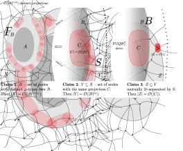
Figure 1: The sets $A$ and $B$ are $2$-separated by $S$.

Observe that taking $r=\infty$ in $r$-separation yields the familiar notion of a separation in graph theory. From the perspective of stability, separation (for $r=\infty$) characterizes forking independence in superflat graphs [19]. Therefore, $r$-separation can be thought of as a local analogue of forking independence, for nowhere dense graph classes.

A key lemma concerning $r$-separation (cf. corollary 16) states that if $A$ and $B$ are $r$-separated by a set $S$ of size $s$ in $G$, then for any fixed formula $\varphi(\bar{x},\bar{y})$ of quantifier rank $\mathcal{O}(\log r)$, the set $\{\{\bar{v}\ \in B^{|\bar{y}|}:G\models\varphi(\bar{u},\bar{v})\}:\bar{u}\in A^{|\bar{x}|}\}$ has cardinality bounded by a constant depending on $s$ and $\varphi$ only (and not on $G,A,$ and $B$). This elementary result combines Gaifman’s locality of first order logic (cf. [15]) and a Feferman-Vaught compositionality argument. This, in combination with the polynomial bounds for uniform quasi-wideness (theorem 6, and its extension to tuples theorem 10), as well as the previous results on neighborhood complexity [11, 13], are the main ingredients of our main result, theorem 4.

A duality theorem.

As an example application of our main result, theorem 4, we prove the following result.

Theorem 7.

Fix a nowhere dense class of graphs $\mathcal{C}$ and a formula $\varphi(x,y)$ with two free variables $x,y$. Then there is a function $f\colon\mathbb{N}\to\mathbb{N}$ with the following property. Let $G\in\mathcal{C}$ be a graph and let $\cal G$ be a family of subsets of $V(G)$ consisting of sets of the form $\left\{v\in V(G)\,\leavevmode\nobreak\ :\leavevmode\nobreak\ \,\varphi(u,v)\right\}$, where $u$ is some vertex of $V(G)$. Then $\tau({\cal G})\leqslant f(\nu(\cal G))$.

Above, $\tau(\cal G)$ denotes the transversality of $\cal G$, i.e., the least number of elements of a set $X$ which intersects every set in $\cal G$, and $\nu(\cal G)$ denotes the packing number of $\cal G$, i.e., the largest number of pairwise-disjoint subsets of $\cal G$. theorem 7 is an immediate consequence of the bound given by theorem 4 and a result of Matoušek [25].

We remark that a similar, but incomparable result is proved by Bousquet and Thomassé [6]. In their result, the assumption on $\mathcal{C}$ is weaker, since they just require that it has bounded distance VC-dimension, but the assumption on $\cal G$ is stronger, as it is required to be the set of all balls of a fixed radius.

Stability.

Finally, we observe that we can apply our tools to give a constructive proof of the result of Adler and Adler [1] that every nowhere dense class is stable, which yields computable upper bounds on ladder indices. More precisely, we translate the approach of Podewski and Ziegler [31] to the finite and replace the key non-constructive application of compactness with a combinatorial argument based on Gaifman’s locality, in the flavor served by our observations on $r$-separation (corollary 16). The following theorem summarizes our result.

Theorem 8.

There are computable functions $f\colon\mathbb{N}^{3}\to\mathbb{N}$ and $g\colon\mathbb{N}\to\mathbb{N}$ with the following property. Suppose $\varphi(\bar{x},\bar{y})$ is a formula of quantifier rank at most $q$ and with $d$ free variables. Suppose further that $G$ is a graph excluding $K_{t}$ as a depth-$g(q)$ minor. Then the ladder index of $\varphi(\bar{x},\bar{y})$ in $G$ is at most $f(q,d,t)$.

Organization.

In section 2 we recall some standard concepts from the theory of sparse graphs. In section 3 we prove theorem 6, improving the previously known bounds and making them constructive. We remark that this result is not needed in the proof of our main result, theorem 4. The following two sections contain the main tools needed in the proof of the main result: in section 4 we formulate and prove the generalization of uniform quasi-wideness to tuples, theorem 10, and in section 5 we discuss Gaifman locality for first order logic and derive an elementary variant concerning local separators. In section 6 we prove our main result, theorem 4, and the corresponding lower bounds, theorem 5. Finally, in section 8 we provide a constructive proof of the result of Adler and Adler, theorem 8.

Acknowledgments.

We would like to thank Patrice Ossona de Mendez for pointing us to the question of studying VC-density of nowhere dense graph classes.

2 Preliminaries

We recall some basic notions from graph theory.

All graphs in this paper are finite, undirected and simple, that is, they do not have loops or parallel edges. Our notation is standard, we refer to [10] for more background on graph theory. We write $V(G)$ for the vertex set of a graph $G$ and $E(G)$ for its edge set. The distance between vertices $u$ and $v$ in $G$, denoted $\mathrm{dist}_{G}(u,v)$, is the length of a shortest path between $u$ and $v$ in $G$. If there is no path between $u$ and $v$ in $G$, we put $\mathrm{dist}_{G}(u,v)=\infty$. The (open) neighborhood of a vertex $u$, denoted $N(u)$, is the set of neighbors of $u$, excluding $u$ itself. For a non-negative integer $r$, by $N_{r}[u]$ we denote the (closed) $r$-neighborhood of $u$ which comprises vertices at distance at most $r$ from $u$; note that $u$ is always contained in its closed $r$-neighborhood. The radius of a connected graph $G$ is the least integer $r$ such that there is some vertex $v$ of $G$ with $N_{r}[v]=V(G)$.

A minor model of a graph $H$ in $G$ is a family $(I_{u})_{u\in V(H)}$ of pairwise vertex-disjoint connected subgraphs of $G$, called branch sets, such that whenever $uv$ is an edge in $H$, there are $u^{\prime}\in V(I_{u})$ and $v^{\prime}\in V(I_{v})$ for which $u^{\prime}v^{\prime}$ is an edge in $G$. The graph $H$ is a depth-$r$ minor of $G$, denoted $H\preccurlyeq_{r}G$, if there is a minor model $(I_{u})_{u\in V(H)}$ of $H$ in $G$ such that each $I_{u}$ has radius at most $r$.

A class $\mathcal{C}$ of graphs is nowhere dense if there is a function $t\colon\mathbb{N}\rightarrow\mathbb{N}$ such that for all $r\in\mathbb{N}$ it holds that $K_{t(r)}\not\preccurlyeq_{r}G$ for all $G\in\mathcal{C}$, where $K_{t(r)}$ denotes the clique on $t(r)$ vertices. The class $\mathcal{C}$ moreover has bounded expansion if there is a function $d\colon\mathbb{N}\rightarrow\mathbb{N}$ such that for all $r\in\mathbb{N}$ and all $H\preccurlyeq_{r}G$ with $G\in\mathcal{C}$, the edge density of $H$, i.e. $|E(H)|/|V(H)|$, is bounded by $d(r)$. Note that every class of bounded expansion is nowhere dense. The converse is not necessarily true in general [29].

A set $B\subseteq V(G)$ is called $r$-independent in a graph $G$ if $\mathrm{dist}_{G}(u,v)>r$ for all distinct $u,v\in B$. A class $\mathcal{C}$ of graphs is uniformly quasi-wide if for every $r\in\mathbb{N}$ there is a number $s\in\mathbb{N}$ and a function $N\colon\mathbb{N}\to\mathbb{N}$ such that for every $m\in\mathbb{N}$, graph $G\in\mathcal{C}$, and vertex subset $A\subseteq V(G)$ of size $\left\lvert A\right\rvert\geqslant N(m)$, there is a set $S\subseteq V(G)$ of size $\left\lvert S\right\rvert\leqslant s$ and a set $B\subseteq A-S$ of size $\left\lvert B\right\rvert\geqslant m$ which is $r$-independent in $G-S$. Recall that Nešetřil and Ossona de Mendez proved [28] that nowhere dense graph classes are exactly the same as uniformly quasi-wide classes. The following result of Kreutzer, Rabinovich and the second author [21] improves their result, by showing that the function $N$ can be taken polynomial:

Theorem 9 ([21]).

For every nowhere dense class $\mathcal{C}$ and for all $r\in\mathbb{N}$ there is a polynomial $N\colon\mathbb{N}\to\mathbb{N}$ and a number $s\in\mathbb{N}$ such that the following holds. Let be $G\in\mathcal{C}$ be aa graph and let $A\subseteq V(G)$ be a vertex subset of size at least $N(m)$, for a given $m$. Then there exists a set $S\subseteq V(G)$ of size $|S|<s$ and a set $B\subseteq A-S$ of size $|B|\geqslant m$ which is $r$-independent in $G-S$.

As we mentioned, the proof of Kreutzer et al. [21] relies on non-constructive arguments and does not yield explicit bounds on $s$ and (the degree of) $N$. In the next section, we discuss a further strengthening of this result, by providing explicit, computable bounds on $N$ and $s$.

3 Bounds for uniform quasi-wideness

In this section we prove theorem 6, which strengthens theorem 9 by providing an explicit polynomial $N$ and bound $s$, whereas the bounds in theorem 9 rely on non-constructive arguments. We note that theorem 9 is sufficient to prove our main result, theorem 4, but is required in our proof of theorem 8, which is the effective variant of the result of Adler and Adler, theorem 8.

General strategy.

Our proof follows the same lines as the original proof of Nešetřil and Ossona de Mendez [28], with the difference that in the key technical lemma (lemma 2 below), we improve the bounds significantly by replacing a Ramsey argument with a refined combinatorial analysis. The new argument essentially originates in the concept of branching index from stability theory.

We first prove a restricted variant, lemma 1 below, in which we assume that $A$ is already $(r-1)$-independent. Then, in order to derive theorem 6, we apply the lemma iteratively for $r$ ranging from $1$ to the target value.

Lemma 1.

For every pair of integers $t,r\in\mathbb{N}$ there exists an integer $d<9r/2$ and a function $L\colon\mathbb{N}\to\mathbb{N}$ with $L(m)=\mathcal{O}_{r,t}{(m^{{(4t+1)}^{2rt}})}$ such that the following holds. For each $m\in\mathbb{N}$, graph $G$ with $K_{t}\not\preccurlyeq_{d}G$, and $(r-1)$-independent set $A\subseteq V(G)$ of size at least $L(m)$, there is a set $S\subseteq V(G)-A$ of size less than $t$ such that $A$ contains a subset $B$ of size $m$ which is $r$-independent in $G-S$. Moreover, if $r$ is odd then $S$ is empty, and if $r$ is even, then every vertex of $S$ is at distance exactly $r/2$ from every vertex of $B$. Finally, given $G$ and $A$, the sets $B$ and $S$ can be computed in time $\mathcal{O}_{r,t}(|A|\cdot|E(G)|)$.

We prove lemma 1 in Section 3.2, but a very rough sketch is as follows. The case of general $r$ reduces to the case $r=1$ or $r=2$, depending on the parity of $r$, by contracting the balls of radius $\lfloor\frac{r-1}{2}\rfloor$ around the vertices in $A$ to single vertices. The case of $r=1$ follows immediately from Ramsey’s theorem, as in [28]. The case $r=2$ is substantially more difficult. We start by formulating and proving the main technical result needed for proving the case $r=2$.

3.1 The main technical lemma

The following, Ramsey-like result is the main technical lemma used in the proof of theorem 6.

Lemma 2.

Let $\ell,m,t\in\mathbb{N}$ and assume $\ell\geqslant t^{8}$. If $G$ is a graph and $A$ is a $1$-independent set in $G$ with at least $(m+\ell)^{2t}$ elements, then at least one of the following conditions hold:

• $K_{t}\preccurlyeq_{4}G$,

• $A$ contains a $2$-independent set of size $m$,

• some vertex $v$ of $G$ has at least $\ell^{1/4}$ neighbors in $A$.

Moreover, if $K_{t}\not\preccurlyeq_{4}G$, the structures described in the other two cases (a $2$-independent set of size $m$, or a vertex $v$ as above) can be computed in time $\mathcal{O}_{t}(|A|\cdot|E(G)|)$.

We remark that a statement similar to that of lemma 2 can be obtained by employing Ramsey’s theorem, as has been done in [28]. This, however, does not give a bound which is polynomial in $m+\ell$, and thus cannot be used to prove theorem 6.

The remainder of this section is devoted to the proof of lemma 2. We will use the following bounds on the edge density of graphs with excluded shallow minors obtained by Alon et al. [3].

Lemma 3 (Theorem 2.2 in [3]).

Let $H$ be a bipartite graph with maximum degree $d$ on one side. Then there exists a constant $c_{H}$, depending only on $H$, such that every $n$-vertex graph $G$ excluding $H$ as a subgraph has at most $c_{H}\cdot n^{2-1/d}$ edges.

Observe that if $K_{t}\not\preccurlyeq_{1}G$, then in particular the $1$-subdivision of $K_{t}$ is excluded as a subgraph of $G$ (the $1$-subdivision of a graph $H$ is obtained by replacing every edge of $H$ by a path of length $2$). Moreover, the $1$-subdivision of $K_{t}$ is a bipartite graph with maximum degree $2$ on one side. Furthermore, it is easy to check in the proof of Theorem 2.2 in [3] that $c_{H}\leqslant|V(H)|$ in case $d=2$. Since the $1$-subdivision of $K_{t}$ has $\binom{t+1}{2}$ vertices, we can choose $c_{K_{t}}=\binom{t+1}{2}$ and conclude the following.

Corollary 4.

Let $G$ be an $n$-vertex graph such that $K_{t}\not\preccurlyeq_{1}G$ for some constant $t\in\mathbb{N}$. Then $G$ has at most $\binom{t+1}{2}\cdot n^{3/2}$ edges.

We will use the following standard lemma saying that a shallow minor of a shallow minor is a shallow minor, where the parameters of shallowness are appropriately chosen.

Lemma 5 (adaptation of Proposition 4.11 in [29]).

Suppose $J,H,G$ are graphs such that $H\preccurlyeq_{a}G$ and $J\preccurlyeq_{b}H$, for some $a,b\in\mathbb{N}$. Then $J\preccurlyeq_{c}G$, where $c=2ab+a+b$.

We will need one more technical lemma.

Lemma 6.

Let $G$ be a graph such that $K_{t}\not\preccurlyeq_{4}G$ for some $t\in\mathbb{N}$ and let $A\subseteq V(G)$ with $|A|\geqslant t^{8}$. Assume furthermore that every pair of elements of $A$ has a common neighbor in $V(G)-A$. Then there exists a vertex $v$ in $V(G)-A$ which has at least $|A|^{1/4}$ neighbors in $A$.

Proof.

Denote $k=\max\{\,|N(w)\cap A|\ \colon\ w\in V(G)-A\,\}$; our goal is to prove that $k\geqslant|A|^{1/4}$.

Let $B\subseteq V(G)-A$ be the set of those vertices outside of $A$ that have a neighbor in $A$. Construct a function $f\colon B\to A$ by a random procedure as follows: for each vertex $v\in B$, choose $f(v)$ uniformly and independently at random from the set $N(v)\cap A$. Next, for each $u\in A$ define branch set $I_{u}=G[\{u\}\cup f^{-1}(u)]$. Observe that since, by construction, $v$ and $f(v)$ are adjacent for all $v\in B$, each branch set $I_{u}$ has radius at most $1$, with $u$ being the central vertex. Also, the branch sets $\{I_{u}\}_{u\in A}$ are pairwise disjoint. Finally, construct a graph $H$ on vertex set $A$ by making distinct $u,v\in A$ adjacent in $H$ whenever there is an edge in $G$ between the branch sets $I_{u}$ and $I_{v}$. Then the branch sets $\{I_{u}\}_{u\in A}$ witness that $H$ is a $1$-shallow minor of $G$.

For distinct $u,v\in A$, let us estimate the probability that the edge $uv$ appears in $H$. By assumption, there is a vertex $w\in B$ that is adjacent both to $u$ and to $v$. Observe that if it happens that $f(w)=u$ or $f(w)=v$, then $uv$ for sure becomes an edge in $H$. Since $w$ has at most $k$ neighbors in $A$, the probability that $f(w)\in\{u,v\}$ is at least $\frac{2}{k}$.

By the linearity of expectation, the expected number of edges in $H$ is at least $\binom{|A|}{2}\cdot\frac{2}{k}=\frac{|A|(|A|-1)}{k}$. Hence, for at least one run of the random experiment we have that $H$ indeed has at least this many edges. On the other hand, observe that $K_{t}\not\preccurlyeq_{1}H$; indeed, since $H\preccurlyeq_{1}G$, by Lemma 5 we infer that $K_{t}\preccurlyeq_{1}H$ would imply $K_{t}\preccurlyeq_{4}G$, a contradiction with the assumptions on $G$. Then Corollary 4 implies $H$ has at most $\binom{t+1}{2}\cdot|A|^{3/2}$ edges. Observe that $\binom{t+1}{2}\cdot|A|^{3/2}\leqslant 3t^{2}/4\cdot|A|^{3/2}\leqslant\frac{3}{4}|A|^{7/4}$, where the first inequality holds due to $t\geqslant 2$, while the second holds by the assumption that $|A|\geqslant t^{8}$. By combining the above bounds, we obtain

$$\frac{|A|(|A|-1)}{k}\leqslant\frac{3}{4}|A|^{7/4},$$

which implies $k\geqslant|A|^{1/4}$ due to $|A|\geqslant t^{8}\geqslant 64$. $\square$

We proceed with the proof of lemma 2. The idea is to arrange the elements of $A$ in a binary tree and prove that provided $A$ is large, this tree contains a long path. From this path, we will extract the set $B$. In stability theory, similar trees are called type trees and they are used to extract long indiscernible sequences, see e.g. [23].

We will work with a two-symbol alphabet $\{\mathrm{D},\mathrm{S}\}$, for daughter and son. We identify words in $\{\mathrm{D},\mathrm{S}\}^{*}$ with nodes of the infinite rooted binary tree. The depth of a node $w$ is the length of $w$. For $w\in\{\mathrm{D},\mathrm{S}\}^{*}$, the nodes $w\mathrm{D}$ and $w\mathrm{S}$ are called, respectively, the daughter and the son of $w$, and $w$ is the parent of both $w\mathrm{S}$ and $w\mathrm{D}$. A node $w^{\prime}$ is a descendant of a node $w$ if $w^{\prime}$ is a prefix of $w$ (possibly $w^{\prime}=w$). We consider finite, labeled, rooted, binary trees, which are called simply trees below, and are defined as follows. For a set of labels $U$, a ($U$-labeled) tree is a partial function $\tau\colon\{\mathrm{D},\mathrm{S}\}^{*}\to U$ whose domain is a finite set of nodes, called the nodes of $\tau$, which is closed under taking parents. If $v$ is a node of $\tau$, then $\tau(v)$ is called its label.

Let $G$ be a graph, $A\subseteq V(G)$ be a $1$-independent set in $G$, and $\bar{a}$ be any enumeration of $A$, that is, a sequence of length $|A|$ in which every element of $A$ appears exactly once. We define a binary tree $\tau$ which is labeled by vertices of $G$. The tree is defined by processing all elements of $\bar{a}$ sequentially. We start with $\tau$ being the tree with empty domain, and for each element $a$ of the sequence $\bar{a}$, processed in the order given by $\bar{a}$, execute the following procedure which results in adding a node with label $a$ to $\tau$.

When processing the vertex $a$, do the following. Start with $w$ being the empty word. While $w$ is a node of $\tau$, repeat the following step: if the distance from $a$ to $\tau(w)$ in the graph $G$ is at most $2$, replace $w$ by its son, otherwise, replace $w$ by its daughter. Once $w$ is not a node of $\tau$, extend $\tau$ by setting $\tau(w)=a$. In this way, we have processed the element $a$, and now proceed to the next element of $\bar{a}$, until all elements are processed. This ends the construction of $\tau$. Thus, $\tau$ is a tree labeled with vertices of $A$, and every vertex of $A$ appears exactly once in $\tau$.

Define the depth of $\tau$ as the maximal depth of a node of $\tau$. For a word $w$, an alternation in $w$ is any position $\alpha$, $1\leqslant\alpha\leqslant|w|$, such that $w_{\alpha}\neq w_{\alpha-1}$; here, $w_{\alpha}$ denotes the $\alpha$th symbol of $w$, and $w_{0}$ is assumed to be $\mathrm{D}$. The alternation rank of the tree $\tau$ is the maximum of the number of alternations in $w$, over all nodes $w$ of $\tau$.

Lemma 7.

Let $h,t\geqslant 2$. If $\tau$ has alternation rank at most $2t-1$ and depth at most $h-1$, then $\tau$ has fewer than $h^{2t}$ nodes.

Proof.

With each node $w$ of $\tau$ associate function $f_{w}\colon\{1,\ldots,2t\}\to\{1,\ldots,h\}$ defined as follows: $f_{w}$ maps each $i\in\{1,\ldots,2t\}$ to the $i$th alternation of $w$, provided $i$ is at most the number of alternations of $w$, and otherwise we put $f_{w}(i)=|w|+1$. It is clear that the mapping $w\mapsto f_{w}$ for nodes $w$ of $\tau$ is injective and its image is contained in monotone functions from $\{1,\ldots,2t\}$ to $\{1,\ldots,h\}$, whose number is less than $h^{2t}$. Hence, the domain of $\tau$ has fewer than $h^{2t}$ elements. $\square$

Lemma 8.

Suppose that $K_{t}\not\preccurlyeq_{2}G$. Then $\tau$ has alternation rank at most $2t-1$.

Proof.

Let $w$ be a node of $\tau$ with at least $2k$ alternations, for some $k\in\mathbb{N}$. Suppose $\alpha_{1},\beta_{1},\ldots,\alpha_{k},\beta_{k}$ be the first $2k$ alternations of $w$. By the assumption that $w_{0}=\mathrm{D}$ we have that $w$ contains symbol $\mathrm{S}$ at all positions $\alpha_{i}$ for $i=1,\ldots,k$, and symbol $\mathrm{D}$ at all positions $\beta_{i}$ for $i=1,\ldots,k$. For each $i\in\{1,\ldots,k\}$, define $a_{i}\in V(G)$ to be the label in $\tau$ of the prefix of $w$ of length $\alpha_{i}-1$, and similarly define $b_{i}\in V(G)$ to be the label in $\tau$ of the prefix of $w$ of length $\beta_{i}-1$. It follows that for each $i\in\{1,\ldots,k\}$, the following assertions hold: the nodes in $\tau$ with labels $b_{i},a_{i+1},b_{i+1},\ldots,a_{k},b_{k}$ are descendants of the son of the node with label $a_{i}$, and the nodes with labels $a_{i+1},b_{i+1},\ldots,a_{k},b_{k}$ are descendants of the daughter of the node with label $b_{i}$.

Claim 1.

For every pair $a_{i},b_{j}$ with $1\leqslant i\leqslant j\leqslant k$, there is a vertex $z_{ij}\not\in A$ which is a common neighbor of $a_{i}$ and $b_{j}$, and is not a neighbor of any $b_{s}$ with $s\neq j$.

Proof.

Note that since $i\leqslant j$, the node with label $b_{j}$ is a descendant of the son of the node with label $a_{i}$, hence we have $\mathrm{dist}_{G}(a_{i},b_{j})\leqslant 2$ by the construction of $\tau$. However, we also have $\mathrm{dist}_{G}(a_{i},b_{j})>1$ since $A$ is $1$-independent. Therefore $\mathrm{dist}_{G}(a_{i},b_{j})=2$, so there is a vertex $z_{ij}$ which is a common neighbor of $a_{i}$ and $b_{j}$. Suppose that $z_{ij}$ was a neighbor of $b_{s}$, for some $s\neq j$. This would imply that $\mathrm{dist}_{G}(b_{j},b_{s})\leqslant 2$, which is impossible, because the nodes with labels $b_{s}$ and $b_{j}$ in $\tau$ are such that one is a descendant of the daughter of the other, implying that $\mathrm{dist}_{G}(b_{s},b_{j})>2$. $\lrcorner$

Note that whenever $i\leqslant j$ and $i^{\prime}\leqslant j^{\prime}$ are such that $j\neq j^{\prime}$, the vertices $z_{ij}$ and $z_{i^{\prime}j^{\prime}}$ are different, because $z_{ij}$ is adjacent to $b_{j}$ but not to $b_{j^{\prime}}$, and the converse holds for $z_{i^{\prime}j^{\prime}}$. However, it may happen that $z_{ij}=z_{i^{\prime}j}$ even if $i\neq i^{\prime}$. This will not affect our further reasoning.

For each $j\in\{1,\ldots,k\}$, let $B_{j}$ be the subgraph of $G$ induced by the set $\{a_{j},b_{j}\}\cup\{z_{ij}\colon 1\leqslant i\leqslant j\}$. Observe that $B_{j}$ is connected and has radius at most $2$, with $b_{j}$ being the central vertex. By lemma 8 and the discussion from the previous paragraph, the graphs $B_{j}$ for $j\in\{1,\ldots,k\}$ are pairwise disjoint. Moreover, for all $1\leqslant i\leqslant j\leqslant k$, there is an edge between $B_{i}$ and $B_{j}$, namely, the edge between $z_{ij}\in B_{j}$ and $a_{i}\in B_{i}$. Hence, the graphs $B_{j}$, for $j\in\{1,\ldots,k\}$, define a depth-$2$ minor model of $K_{k}$ in $G$. Since $K_{t}\not\preccurlyeq_{2}G$, this implies that $k<t$, proving lemma 8. $\square$

We continue with the proof of lemma 2. Fix integers $\ell\geqslant t^{8}$ and $m$, and define $h=m+\ell$. Let $A$ be a $1$-independent set in $G$ of size at least $h^{2t}$.

Suppose that the first case of lemma 2 does not hold. In particular $K_{t}\not\preccurlyeq_{2}G$, so by lemma 8, $\tau$ has alternation rank at most $2t-1$. From lemma 7 we conclude that $\tau$ has depth at least $h$. As $h=m+\ell$, it follows that either $\tau$ has a node $w$ which contains at least $m$ letters $\mathrm{D}$, or $\tau$ has a node $w$ which contains at least $\ell$ letters $\mathrm{S}$.

Consider the first case, i.e., there is a node $w$ of $\tau$ which contains at least $m$ letters $\mathrm{D}$, and let $X$ be the set of all vertices $\tau(u)$ such that $u\mathrm{D}$ is a prefix of $w$. Then, by construction, $X$ is a $2$-independent set in $G$ of size at least $m$, so the second case of the lemma holds.

Finally, consider the second case, i.e., there is a node $w$ in $\tau$ which contains at least $\ell$ letters $\mathrm{S}$. Let $Y$ be the set of all vertices $\tau(u)$ such that $u\mathrm{S}$ is a prefix of $w$. Then, by construction, $Y\subseteq A$ is a set of at least $\ell$ vertices which are mutually at distance exactly $2$ in $G$. Since $K_{t}\not\preccurlyeq_{4}G$ and $\ell\geqslant t^{8}$, by lemma 6 we infer that there is a vertex $v\in G$ with at least $\ell^{1/4}$ neighbors in $Y$. This finishes the proof of the existential part of lemma 2.

For the algorithmic part, the proof above yields an algorithm which first constructs the tree $\tau$, by iteratively processing each vertex $w$ of $A$ and testing whether the distance between $w$ and each vertex processed already is equal to $2$. This amounts to running a breadth-first search from every vertex of $A$, which can be done in time $\mathcal{O}(|A|\cdot|E(G)|)$. Whenever a node with $2t$ alternations is inserted to $\tau$, we can exhibit in $G$ a depth-$2$ minor model of $K_{t}$. Whenever a node with least $m$ letters $\mathrm{D}$ is added to $\tau$, we have constructed an $m$-independent set. Whenever a node with at least $\ell$ letters $\mathrm{S}$ is added to $\tau$, as argued, there must be some vertex $v\in V(G)-A$ with at least $\ell^{1/8}$ neighbors in $A$. To find such a vertex, scan through all neighborhoods of vertices $v\in A$ in the graph $G$, and then select a vertex $w\in V(G)$ which belongs to the largest number of those neighborhoods; this can be done in time $\mathcal{O}(|E(G)|)$. The overall running time is $\mathcal{O}(|A|\cdot|E(G)|)$, as required.

3.2 Proof of lemma 1

With lemma 2 proved, we can proceed with lemma 1. We start with the case $r=1$, then we move to the case $r=2$. Next, we show how the general case reduces to one of those two cases.

Case $r=1$.

We put $d=0$, thus we assume that $K_{t}\not\preccurlyeq_{0}G$; that is, $G$ does not contain a clique of size $t$ as a subgraph. By Ramsey’s Theorem, in every graph every vertex subset of size $\binom{m+t-2}{t-1}$ contains an independent set of size $m$ or a clique of size $t$. Therefore, taking $L(m)$ to be the above binomial coefficient yields lemma 1 in case $r=0$, for $S=\emptyset$. Note here that $\binom{m+t-2}{t-1}\in\mathcal{O}_{t}{(m^{{(4t+1)}^{2t}})}$. Moreover, such independent set or clique can be computed from $G$ and $A$ in time $\mathcal{O}(|A|\cdot|E(G)|)$ by simulating the proof of Ramsey’s theorem.

Case $r=2$.

We put $d=2$, thus we assume that $K_{t}\not\preccurlyeq_{4}G$. We show that if $A$ is a sufficiently large $1$-independent set in a graph $G$ such that $K_{t}\not\preccurlyeq_{4}G$, then there is a set of vertices $S$ of size less than $t$ such that $A-S$ contains a subset of size $m$ which is $2$-independent in $G-S$. Here, by “sufficiently large” we mean of size of size at least $L(m)$, for $L(m)$ emerging from the proof. To this end, we shall iteratively apply lemma 2 as long as it results in the third case, yielding a vertex $v$ with many neighbors in $A$. In this case, we add $v$ vertex to the set $S$, and apply the lemma again, restricting $A$ to $A\cap N(v)$. Precise calculations follow.

Fix a number $\beta>4t$. For $k\geqslant 0$, define $m_{k}=((k+1)\cdot m)^{(2\beta)^{k}}$. In the following we will always assume that $m\geqslant t^{8}$. We will apply lemma 2 in the following form.

Claim 2.

If $G$ is a graph such that $K_{t}\not\preccurlyeq_{4}G$, and $A\subseteq V(G)$ is an $1$-independent set in $G$ which does not contain a $2$-independent set of size $m$ and satisfies $|A|\geqslant m_{k}$, for some $k\geqslant 1$, then there exists a vertex $v\in V(G)-A$ such that $|N_{G}(v)\cap A|\geqslant m_{k-1}$.

Proof.

Let $\ell=(k\cdot m)^{4\cdot(2\beta)^{k-1}}$. Then $m\geqslant t^{8}$ implies that $\ell\geqslant t^{8}$. Observe that

$$|A|\geqslant\left((k+1)\cdot m\right)^{(2\beta)^{k}}\geqslant\left((m+k\cdot m)^{4\cdot(2\beta)^{k-1}}\right)^{2t}\geqslant\left(m+(k\cdot m)^{4\cdot(2\beta)^{k-1}}\right)^{2t}=(m+\ell)^{2t}.$$

Therefore, we may apply lemma 2, yielding a vertex $v$ with at least $\ell^{1/4}=(k\cdot m)^{(2\beta)^{k-1}}=m_{k-1}$ neighbors in $A$. $\lrcorner$

We will now find a subset of $A$ of size $m$ which is $2$-independent in $G-S$, for some $S$ with $|S|<t$. Assume that $|A|\geqslant m_{t}$. By induction, we construct a sequence $A=A_{0}\supseteq A_{1}\supseteq\ldots$ of $1$-independent vertex subsets of $G$ of length at most $t$ such that $|A_{i}|\geqslant m_{t-i}$, as follows. Start with $A_{0}=A$. We maintain a set $S$ of vertices of $G$ which is initially empty, and we maintain the invariant that $A_{i}$ is disjoint with $S$ at each step of the construction.

For $i=0,1,2,\ldots$ do as follows. If $A_{i}$ contains a subset of size $m$ which is $2$-independent set in $G-S$, terminate. Otherwise, apply 2 to the graph $G-S$ with $1$-independent set $A_{i}$ of size $|A_{i}|\geqslant m_{t-i}$. This yields a vertex $v_{i+1}\in V(G)-(S\cup A_{i})$ whose neighborhood in $G-S$ contains at least $m_{t-i-1}$ vertices of $A_{i}$. Define $A_{i+1}$ as the set of neighbors of $v_{i+1}$ in $A_{i}$, and add $v_{i+1}$ to the set $S$. Increment $i$ and repeat.

Claim 3.

The construction halts after less than $t$ steps.

Proof.

Suppose that the construction proceeds for $k\leqslant t$ steps. By construction, each vertex $v_{i}$, for $i\leqslant k$, is adjacent in $G$ to all the vertices of $A_{j}$, for each $i\leqslant j\leqslant k$. In particular, all the vertices $v_{1},\ldots,v_{k}$ are adjacent to all the vertices of $A_{k}$ and $|A_{k}|\geqslant m_{t-k}\geqslant m\geqslant t$. Choose any pairwise distinct vertices $w_{1},\ldots,w_{k}\in A_{k}$ and observe that the connected subgraphs $G[\{w_{i},v_{i}\}]$ of $G$ yield a depth-$1$ minor model of $K_{k}$ in $G$. Since $K_{t}\not\preccurlyeq_{2}G$, we must have $k<t$. $\lrcorner$

Therefore, at some step $k<t$ of the construction we must have obtained a $2$-independent subset $B$ of $G-S$ of size $m$. Moreover, $|S|\leqslant k<t$.

This proves lemma 1 in the case $r=2$, for the function $L(m)$ defined as $L(m)=m_{t}=((t+1)\cdot m)^{\beta^{2t}}$ for $m\geqslant t^{8}$, and $L(m)=L(t^{8})$ for $m<t^{8}$, where $\beta>4t$ is any fixed constant. It is easy to see that then $L(m)\in\mathcal{O}_{t}{(m^{{(4t+1)}^{2t}})}$, provided we put $\beta=4t+1$. Also, the proof easily yields an algorithm constructing the sets $B$ and $S$, which amounts to applying at most $t$ times the algorithm of lemma 2. Hence, its running time is $\mathcal{O}_{r,t}(|A|\cdot|E(G)|)$, as required.

Odd case.

We now prove lemma 1 in the case when $r=2s+1$, for some integer $s\geqslant 1$. We put $d=s=\frac{r-1}{2}$. Let $G$ be a graph such that $K_{t}\not\preccurlyeq_{s}G$, and let $A$ be a $2s$-independent set in $G$. Consider the graph $G^{\prime}$ obtained from $G$ by contracting the (pairwise disjoint) balls of radius $s$ around each vertex $v\in A$. Let $A^{\prime}$ denote the set of vertices of $G^{\prime}$ corresponding to the contracted balls. There is a natural correspondence (bijection) between $A$ and $A^{\prime}$, where each vertex $v\in A$ is associated with the vertex of $A^{\prime}$ resulting from contracting the ball of radius $s$ around $v$. From $K_{t}\not\preccurlyeq_{s}G$ it follows that $G^{\prime}$ does not contain $K_{t}$ as a subgraph. Applying the already proved case $r=1$ to $G^{\prime}$ and $A^{\prime}$, we conclude that provided $|A|=|A^{\prime}|\geqslant{m+t-2\choose t-1}$, the set $A^{\prime}$ contains a $1$-independent subset $B^{\prime}$ of size $m$, which corresponds to a $(2s+1)$-independent set $B$ in $G$ that is contained in $A$; thus, we may put $S=\emptyset$ again. Hence, the obtained bound is $L(m)={m+t-2\choose t-1}$, and we have already argued that then $L(m)\in\mathcal{O}_{r,t}{(m^{{(4t+1)}^{2t}})}$.

Even case.

Finally, we prove lemma 1 in the case $r=2s+2$, for some integer $s\geqslant 1$. We put $d=9s+4=9r/2-5$. Let $G$ be such that $K_{t}\not\preccurlyeq_{d}G$, and let $A$ be a $(2s+1)$-independent set in $G$. Consider the graph $G^{\prime}$ obtained from $G$ by contracting the (pairwise disjoint) balls of radius $s$ around each vertex $v\in A$. Let $A^{\prime}$ denote the set of vertices of $G^{\prime}$ corresponding to the contracted balls. Again, there is a natural correspondence (bijection) between $A$ and $A^{\prime}$. Note that this time, $A^{\prime}$ is a $1$-independent set in $G^{\prime}$. Since $G^{\prime}\preccurlyeq_{s}G$, from $K_{t}\not\preccurlyeq_{9s+4}G$ it follows by Lemma 5 that $K_{t}\not\preccurlyeq_{4}G^{\prime}$. Apply the already proved case $r=2$ to $G^{\prime}$ and $A^{\prime}$. Then, provided $|A|=|A^{\prime}|\geqslant L_{t}(m)$, where $L_{t}(m)$ is the function as defined in the case $r=2$, we infer that $A^{\prime}$ contains a subset $B^{\prime}$ of size $m$ which is $2$-independent in $G^{\prime}-S^{\prime}$, for some $S^{\prime}\subseteq V(G^{\prime})-A^{\prime}$ of size less than $t$. Since $S^{\prime}\cap A^{\prime}=\emptyset$, each vertex of $S^{\prime}$ originates from a single vertex of $G$ before the contractions yielding $G^{\prime}$; thus, $S^{\prime}$ corresponds to a set $S$ consisting of less than $t$ vertices of $G$ which are at distance at least $s+1$ from each vertex in $A$. In turn, the set $B^{\prime}$ corresponds to some subset $B$ of $A$ which is $(2s+2)$-independent in $G-S$. Moreover, as in $G^{\prime}$ each vertex of $S^{\prime}$ is a neighbor of each vertex of $B^{\prime}$, each vertex of $S$ has distance exactly $s+1=r/2$ from each vertex of $B$.

An algorithm computing the sets $B$ and $S$ (in either the odd or even case) can be given as follows: simply run a breadth-first search from each vertex of $A$ to compute the graph $G^{\prime}$ with the balls of radius $\lfloor\frac{r-1}{2}\rfloor$ around the vertices in $A$ contracted to single vertices, and then run the algorithm for the case $r=1$ or $r=2$. This yields a running time of $\mathcal{O}_{r,t}(|A|\cdot|E(G)|)$.

This finishes the proof of lemma 1.

3.3 Proof of theorem 6

We now wrap up the proof of theorem 6 by iteratively applying lemma 1. We repeat the statement for convenience.

Theorem 6.

For all $r,t\in\mathbb{N}$ there is a polynomial $N\colon\mathbb{N}\to\mathbb{N}$ with $N(m)=\mathcal{O}_{r,t}{(m^{{(4t+1)}^{2rt}})}$, such that the following holds. Let $G$ be a graph such that $K_{t}\not\preccurlyeq_{\lfloor 9r/2\rfloor}G$, and let $A\subseteq V(G)$ be a vertex subset of size at least $N(m)$, for a given $m$. Then there exists a set $S\subseteq V(G)$ of size $|S|<t$ and a set $B\subseteq A-S$ of size $|B|\geqslant m$ which is $r$-independent in $G-S$. Moreover, given $G$ and $A$, such sets $S$ and $B$ can be computed in time $\mathcal{O}_{r,t}(|A|\cdot|E(G)|)$.

Proof.

Fix integers $r,t$, and a graph $G$ such that $K_{t}\not\preccurlyeq_{d}G$, for $d=\lfloor 9r/2\rfloor$. Let $\beta>4t$ be a fixed real. As in the proof of lemma 1, we suppose $m\geqslant t^{8}$; this will be taken care by the final choice of the function $N(m)$. Denote $\gamma=\beta^{2t}$, and define the function $L(m)$ as $L(m)=((t+1)\cdot m)^{\gamma}$.

Define sequence $m_{0},m_{1},\ldots,m_{r}$ as follows:

$$m_{r} = m$$

$$m_{i} = L(m_{i+1})\qquad\textrm{for }0\leqslant i<m.$$

A straightforward induction yields that

$$m_{i}=(t+1)^{\frac{\gamma^{r-i}-1}{\gamma-1}}\cdot m^{\gamma^{r-i}}\qquad\textrm{for all }i\in\{0,\ldots,r\}.$$

Suppose that $A$ is a set of vertices of $G$ such that $|A|\geqslant m_{0}=(t+1)^{\frac{\gamma^{r}-1}{\gamma-1}}\cdot m^{\gamma^{r}}$. We inductively construct sequences of sets $A=A_{0}\supseteq A_{1}\supseteq\ldots\supseteq A_{r}$ and $\emptyset=S_{0}\subseteq S_{1}\subseteq S_{2}\ldots$ satisfying the following conditions:

• $|A_{i}|\geqslant m_{i}=L(m_{i+1})$,

• $A_{i}\cap S_{i}=\emptyset$ and $A_{i}$ is $i$-independent in $G-S_{i}$.

To construct $A_{i+1}$ out of $A_{i}$, apply lemma 1 to the graph $G-S_{i}$ and the $i$-independent set $A_{i}$ of size at least $L(m_{i+1})$. This yields a set $S\subseteq V(G)$ which is disjoint from $S_{i}\cup A_{i}$, and a subset $A_{i+1}$ of $A_{i}-S$ of size at least $m_{i+1}$ which is $(i+1)$-independent in $G-S_{i+1}$, where $S_{i+1}=S\cup S_{i}$. This completes the inductive construction.

In particular, $|A_{r}|\geqslant m_{r}=m$ and $A_{r}$ is a subset of $A$ which is $r$-independent in $G-S_{r}$. Observe that by construction, $|S_{r}|<rt/2$, as in the odd steps, the constructed set $S$ is empty, and in the even steps, it has less than $t$ elements. We show that in fact we have $|S_{r}|<t$ using the following argument, similar to the one used in 3.

By the last part of the statement of lemma 1, at the $i$th step of the construction, each vertex of the set $S$ obtained from lemma 1 is at distance exactly $i/2$ from all the vertices in $A_{i+1}$ in the graph $G-S_{i}$. For $a\in A_{r}$, let $\overline{N}(a)$ denote the $\lfloor r/2\rfloor$-neighborhood of $a$ in $G-S_{r}$; note that sets $\overline{N}(a)$ are pairwise disjoint. The above remark implies that each vertex $v$ of the final set $S_{r}$ has a neighbor in the set $\overline{N}(a)$ for each $a\in A_{r}$. Indeed, suppose $v$ belonged to the set $S$ added to $S_{r}$ in the $i$th step of the construction; i.e. $v\in S_{i+1}-S_{i}$. Then there exists a path in $G-S_{i}$ from $v$ to $a$ of length exactly $i/2$, which traverses only vertices at distance less than $i/2$ from $a$. Since in this and further steps of the construction we were removing only vertices at distance at least $i/2$ from $a$, this path stays intact in $G-S_{r}$ and hence is completely contained in $\overline{N}(a)$.

By assumption that $m\geqslant t$, we may choose pairwise different vertices $a_{1},\ldots,a_{t}\in A_{r}$. To reach a contradiction, suppose that $S_{r}$ contains $t$ distinct vertices $s_{1},\ldots,s_{t}$. By the above, the sets $\overline{N}(a_{i})\cup\{s_{i}\}$ form a minor model of $K_{t}$ in $G$ at depth-$(\lfloor r/2\rfloor+1)$. This contradicts the assumption that $K_{t}\not\preccurlyeq_{d}G$ for $d=\lfloor 9r/2\rfloor$. Hence, $|S|<t$.

Define the function $N:\mathbb{N}\to\mathbb{N}$ as $N(m)=(t+1)^{\frac{\gamma^{r}-1}{\gamma-1}}\cdot m^{\gamma^{r}}$ for $m\geqslant t^{8}$ and $N(m)=N(t^{8})$ for $m<t^{8}$; this justifies the assumption $m\geqslant t^{8}$ made in the beginning. Recalling that $\gamma=\beta^{2t}$ and putting $\beta=4t+1$, we note that $N(m)\in\mathcal{O}_{r,t}{(m^{{(4t+1)}^{2rt}})}$. The argument above shows that if $|A|\geqslant N(m)$, then there is a set $S\subseteq V(G)$, equal to $S_{r}$ above, and a set $B\subseteq A$, equal to $A_{r}$ above, so that $B$ is $r$-independent in $G-S$. Given $G$ and $A$, the sets $S$ and $B$ can be computed by applying the algorithm of lemma 1 at most $r$ times, so in time $\mathcal{O}_{r,t}(|A|\cdot|E(G)|)$. This finishes the proof of theorem 6. $\square$

4 Uniform quasi-widness for tuples

We now formulate and prove an extension of theorem 6 which applies to sets of tuples of vertices, rather than sets of vertices. This more general result will be used later on in the paper. The result and its proof are essentially adaptations to the finite of their infinite analogues introduced by Podewski and Ziegler (cf. [31], Corollary 3), modulo the numerical bounds.

We generalize the notion of independence to sets of tuples of vertices. Fix a graph $G$ and a number $r\in\mathbb{N}$, and let $S\subseteq V(G)$ be a subset of vertices of $G$. We say that vertices $u$ and $v$ are $r$-separated by $S$ in $G$ if every path of length at most $r$ connecting $u$ and $v$ in $G$ passes through a vertex of $S$. We extend this notion to tuples: two tuples $\bar{u},\bar{v}$ of vertices of $G$ are $r$-separated by $S$ every vertex appearing in $\bar{u}$ is $r$-separated by $S$ from every vertex appearing in $\bar{v}$. Finally, if $A\subseteq V(G)^{d}$ is a set of $d$-tuples of vertices, for some $d\in\mathbb{N}$, then we say that $A$ is mutually $r$-separated by $S$ in $G$ if any two distinct $\bar{u},\bar{v}\in A$ are $r$-separated by $S$ in $G$.

With these definitions set, we may introduce the notion of uniform quasi-wideness for tuples.

Definition 1.

Fix a class $\cal C$ and numbers $r,d\in\mathbb{N}$. For a function $N\colon\mathbb{N}\to\mathbb{N}$ and number $s\in\mathbb{N}$, we say that $\cal C$ satisfies property $\mathrm{UQW}^{d}_{r}(N,s)$ if the following condition holds:

for every $m\in\mathbb{N}$ and every subset $A\subseteq V(G)^{d}$ with $|A|\geqslant N(m)$, there is a set $S\subseteq V(G)$ with $|S|\leqslant s$ and a subset $B\subseteq A$ with $|B|\geqslant m$ which is mutually $r$-separated by $S$ in $G$.

We say that $\cal C$ satisfies property $\mathrm{UQW}^{d}_{r}$ if $\cal C$ satisfies $\mathrm{UQW}^{d}_{r}(N,s)$ for some $N\colon\mathbb{N}\to\mathbb{N}$ and $s\in\mathbb{N}$. If moreover one can take $N$ to be a polynomial, then we say that $\cal C$ satisfies property $\mathrm{PUQW}^{d}_{r}$.

When $d=1$, we omit it from the superscripts. Note that there is a slight discrepancy in the definition of uniform quasi-wideness and the property of satisfying $\mathrm{UQW}_{r}$, for all $r\in\mathbb{N}$. This is due to the fact that in the original definition, the set $B$ must be disjoint from $S$, whereas in the property $\mathrm{UQW}_{r}$, some vertices of $S$ may belong to $B$. This distinction is inessential when it comes to dimension $1$, since $|S|\leqslant s_{r}$ for some constant $s_{r}$, so passing from one definition to the other requires modifying the function $N_{r}$ by an additive constant $s_{r}$. In particular, a class of graphs $\cal C$ is uniformly quasi-wide if and only if it satisfies $\mathrm{UQW}_{r}$, for all $r\in\mathbb{N}$. However, generalizing to tuples of dimension $d$ requires the use of the definition above, where the tuples in $B$ are allowed to contain vertices which occur in $S$. For example, if the graph $G$ is a star with many arms and $A$ consists of all pairs of adjacent vertices in $G$, then $S$ needs to contain the central vertex of $G$, and therefore $S$ will contain a vertex from every tuple in $A$. We may take $B$ to be equal to $A$ in this case.

Using the above terminology, theorem 6 states that for every fixed $r\in\mathbb{N}$, if there is a number $t\in\mathbb{N}$ such that $K_{t}\not\preccurlyeq_{\lfloor 9r/2\rfloor}G$ for all $G\in\cal C$, then $\cal C$ satisfies $\mathrm{PUQW}_{r}$, and more precisely $\mathrm{UQW}_{r}(N_{r},s_{r})$ for a polynomial $N_{r}\colon\mathbb{N}\to\mathbb{N}$ and number $s_{r}\in\mathbb{N}$, where $N_{r}$ and $s_{r}$ can be computed from $r$ and $t$. The following result provides a generalization to higher dimensions.

Theorem 10.

If $\cal C$ is a nowhere dense class of graphs, then for all $r,d\in\mathbb{N}$, the class $\cal C$ satisfies $\mathrm{PUQW}^{d}_{r}$. More precisely, for any class of graphs $\cal C$ and numbers $r,t\in\mathbb{N}$, if $K_{t}\not\preccurlyeq_{18r}G$ for all $G\in\cal C$, then for all $d\in\mathbb{N}$ the class $\cal C$ satisfies $\mathrm{UQW}^{d}_{r}(N^{d}_{r},s^{d}_{r},)$ for some number $s^{d}_{r}\in\mathbb{N}$ and polynomial $N^{d}_{r}\colon\mathbb{N}\to\mathbb{N}$ that can be computed given $r$, $t$, and $d$.

theorem 10 is an immediate consequence of theorem 6 (or theorem 9 if only the first part of the statement is concerned) and of the following result.

Proposition 9.

For all $r,d\in\mathbb{N}$, if $\cal C$ satisfies $\mathrm{UQW}_{2r}(N_{2r},s_{2r})$ for some $s_{2r}\in\mathbb{N}$ and $N_{2r}\colon\mathbb{N}\to\mathbb{N}$, then $\cal C$ satisfies $\mathrm{UQW}^{d}_{r}(N^{d}_{r},s^{d}_{r})$ for $s^{d}_{r}=d\cdot s_{2r}$ and function $N^{d}_{r}\colon\mathbb{N}\to\mathbb{N}$ defined as $N^{d}_{r}(m)=f^{d}((d^{2}+1)\cdot m)$, where $f(m^{\prime})=m^{\prime}\cdot N_{2r}(m^{\prime})$ and $f^{d}$ is the $d$-fold composition of $f$ with itself.

The rest of section 4 is devoted to the proof of proposition 9. Fix a class $\cal C$ such that $\mathrm{UQW}_{2r}(N_{2r},s_{2r})$ holds for some number $s_{2r}\in\mathbb{N}$ and function $N_{2r}\colon\mathbb{N}\to\mathbb{N}$. We also fix the function $f$ defined in the statement of proposition 9.

Let us fix dimension $d\in\mathbb{N}$, radius $r\in\mathbb{N}$, and graph $G\in\cal C$. For a coordinate $i\in\{1,\ldots,d\}$, by $\pi_{i}\colon V(G)^{d}\to V(G)$ we denote the projection onto the $i$th coordinate; that is, for $\bar{x}\in V(G)^{d}$ by $\pi_{i}(\bar{x})$ we denote the $i$th coordinate of $\bar{x}$.

Our first goal is to find a large subset of tuples that are mutually $2r$-separated by some small $S$ on each coordinate separately. Note that in the following statement we ask for $2r$-separation, instead of $r$-separation.

Lemma 10.

For all $r,m\in\mathbb{N}$ and $A\subseteq V(G)^{d}$ with $|A|\geqslant f^{d}(m)$, there is a set $B\subseteq A$ with $|B|\geqslant m$ and a set $S\subseteq V(G)$ with $|S|\leqslant d\cdot s_{2r}$ such that for each coordinate $i\in\{1,\ldots,d\}$ and all distinct $\bar{x},\bar{y}\in B$, the vertices $\pi_{i}(\bar{x})$ and $\pi_{i}(\bar{y})$ are $2r$-separated by $S$.

Proof.

We will iteratively apply the following claim.

Claim 4.

Fix a coordinate $i\in\{1,\ldots,d\}$, an integer $m^{\prime}\in\mathbb{N}$, and a set $A^{\prime}\subseteq V(G)^{d}$ with $|A^{\prime}|\geqslant f(m^{\prime})$. Then there is a set $B^{\prime}\subseteq A^{\prime}$ with $|B^{\prime}|\geqslant m^{\prime}$ and a set $S^{\prime}\subseteq V(G)$ with $|S^{\prime}|\leqslant s_{2r}$, such that for all distinct $\bar{x},\bar{y}\in B$, the vertices $\pi_{i}(\bar{x})$ and $\pi_{i}(\bar{y})$ are $2r$-separated by $S$.

Proof.

We consider two cases, depending on whether $|\pi_{i}(A^{\prime})|\geqslant N_{2r}(m^{\prime})$.

Suppose first that $\pi_{i}(A^{\prime})$ contains at least $N_{2r}(m^{\prime})$ distinct vertices. Then we may apply the property $\mathrm{UQW}_{2r}$ to $\pi_{i}(A^{\prime})$, yielding sets $S^{\prime}\subseteq V(G)$ and $X\subseteq\pi_{i}(A^{\prime})$ such that $|X|\geqslant m^{\prime}$, $|S^{\prime}|\leqslant s_{2r}$, and $X$ is mutually $2r$-separated by $S^{\prime}$ in $G$. Let $B^{\prime}\subseteq A^{\prime}$ be a subset of tuples constructed as follows: for each $u\in X$, include in $B^{\prime}$ one arbitrarily chosen tuple $\bar{x}\in A^{\prime}$ such that the $i$th coordinate of $\bar{x}$ is $u$. Clearly $|B^{\prime}|=|X|\geqslant m^{\prime}$ and for all distinct $\bar{x},\bar{y}\in B^{\prime}$, we have that $\pi_{i}(\bar{x})$ and $\pi_{i}(\bar{y})$ are different and $2r$-separated by $S^{\prime}$ in $G$; this is because $X$ is mutually $2r$-separated by $S^{\prime}$ in $G$. Hence $B^{\prime}$ and $S^{\prime}$ satisfy all the required properties.

Suppose now that $|\pi_{i}(A^{\prime})|<N_{2r}(m^{\prime})$. Then choose a vertex $a\in\pi_{i}(A^{\prime})$ for which the pre-image $\pi_{i}^{-1}(a)$ has the largest cardinality. Since $|A^{\prime}|\geqslant f(m^{\prime})=m^{\prime}\cdot N_{2r}(m^{\prime})$, we have that

$$|\pi_{i}^{-1}(a)|\geqslant\frac{|A^{\prime}|}{|\pi_{i}(A^{\prime})|}\geqslant\frac{m^{\prime}\cdot N_{2r}(m^{\prime})}{N_{2r}(m^{\prime})}=m^{\prime}.$$

Hence, provided we set $S^{\prime}=\{a\}$ and $B^{\prime}=\pi_{i}^{-1}(a)$, we have that $B^{\prime}$ is mutually $2r$-separated by $S^{\prime}$, $|B^{\prime}|\geqslant m$, and $|S^{\prime}|=1$. $\lrcorner$

We proceed with the proof of lemma 10. Let $A\subseteq V(G)^{d}$ be such that $|A|\geqslant f^{d}(m)$. We inductively define subsets $B_{0}\supseteq B_{1}\supseteq\ldots\supseteq B_{d}$ of $A$ and sets $S_{1},\ldots,S_{d}\subseteq V(G)$ as follows. First put $B_{0}=A$. Then, for each $i=1,\ldots,d$, let $B_{i}$ and $S_{i}$ be the $B^{\prime}$ and $S^{\prime}$ obtained from 4 applied to the set of tuples $B_{i-1}\subseteq V(G)^{d}$, the coordinate $i$, and $m^{\prime}=f^{d-i}(m)$. It is straightforward to see that the following invariant holds for each $i\in\{1,\ldots,d\}$: $|B_{i}|\geqslant f^{d-i}(m)$ and for all $j\leqslant i$ and distinct $\bar{x},\bar{y}\in B_{i}$, the vertices $\pi_{j}(\bar{x})$ and $\pi_{j}(\bar{y})$ are $2r$-separated by $S_{1}\cup\ldots\cup S_{i}$ in $G$. In particular, by taking $B=B_{d}$ and $S=S_{1}\cup\ldots\cup S_{d}$, we obtain that $|B|\geqslant m$, $|S|\leqslant d\cdot s_{2r}$, and $B$ and $S$ satisfy the condition requested in the lemma statement. $\square$

The next lemma will be used to turn mutual $2r$-separation on each coordinate to mutual $r$-separation of the whole tuple set.

Lemma 11.

Let $B\subseteq V(G)^{d}$ and $S\subseteq V(G)$ be such that for each $i\in\{1,\ldots,d\}$ and all distinct $\bar{x},\bar{y}\in B$, the vertices $\pi_{i}(\bar{x})$ and $\pi_{i}(\bar{y})$ are $2r$-separated by $S$ in $G$. Then there is a set $C$ with $C\subseteq B$ and $|C|\geqslant\frac{|B|}{d^{2}+1}$ such that $C$ is mutually $r$-separated by $S$ in $G$.

Proof.

Let $C$ be a maximal subset of $B$ that is mutually $r$-separated by $S$ in $G$. By the maximality of $C$, with each tuple $\bar{a}\in B-C$ we may associate a tuple $\bar{b}\in C$ and a pair of indices $(i,j)\in\{1,\ldots,d\}^{2}$ that witness that $a$ cannot be added to $C$, namely $\pi_{i}(\bar{a})$ and $\pi_{j}(\bar{b})$ are not $r$-separated by $S$ in $G$. Observe that two different tuples $\bar{a},\bar{a}^{\prime}\in B-C$ cannot be associated with exactly the same $\bar{b}\in C$ and same pair of indices $(i,j)$. Indeed, then both $\pi_{i}(\bar{a})$ and $\pi_{i}(\bar{a}^{\prime})$ would not be $r$-separated from $\pi_{j}(\bar{b})$ by $S$ in $G$, which would imply that $\pi_{i}(\bar{a})$ and $\pi_{i}(\bar{a}^{\prime})$ would not be $2r$-separated from each other by $S$, a contradiction with the assumption on $B$. Hence, $|B-C|$ is upper bounded by the number of tuples of the form $(\bar{b},i,j)\in C\times\{1,\ldots,d\}^{2}$, which is $d^{2}|C|$. We conclude that $|B-C|\leqslant d^{2}|C|$, which implies $|C|\geqslant\frac{|B|}{d^{2}+1}$. $\square$

To finish the proof of proposition 9, given a set $A\subseteq V(G)^{d}$ and integer $m\in\mathbb{N}$, first apply lemma 10 with $m^{\prime}=m\cdot(d^{2}+1)$. Assuming that $|A|\geqslant f^{d}(m^{\prime})$, we obtain a set $B\subseteq A$ with $|B|\geqslant m\cdot(d^{2}+1)$ and a set $S\subseteq V(G)$ with $|S|\leqslant d\cdot s_{2r}$, such that for each $i\in\{1,\ldots,d\}$ and all distinct $\bar{x},\bar{y}\in B$, the vertices $\pi_{i}(\bar{x})$ and $\pi_{i}(\bar{y})$ are $2r$-separated by $S$ in $G$. Then, apply lemma 11 to $B$ and $S$, yielding a set $C\subseteq B$ which is mutually $r$-separated by $S$ and has size at least $m$. This concludes the proof of proposition 9.

5 Types and locality

In this section, we develop auxiliary tools concerning first order logic on graphs, in particular we develop a convenient abstraction for Gaifman’s locality property that can be easily combined with the notion of $r$-separation. We begin by recalling some standard notions from logic.

5.1 Logical notions

Formulas.

All formulas in this paper are first order formulas on graph, i.e., they are built using variables (denoted $x,y,z$, etc.), atomic predicates $x=y$ or $E(x,y)$, where the latter denotes the existence of an edge between two nodes, quantifiers $\forall x,\exists x$, and boolean connectives $\lor,\land,\neg$. Let $\varphi(\bar{x})$ be a formula with free variables $\bar{x}$. (Formally, the free variables form a set. To ease notation, we identify this set with a tuple by fixing any its enumeration.) If $\bar{w}\in V^{|\bar{x}|}$ is a tuple of vertices of some graph $G=(V,E)$ (treated as a valuation of the free variables $\bar{x}$), then we write $G,\bar{w}\models\varphi(\bar{x})$ to denote that the valuation $\bar{w}$ satisfies the formula $\varphi$ in the graph $G$. The following example should clarify our notation.

Example 12.

The formula

$$\varphi(x,y)\equiv\exists z_{1}\,\exists z_{2}\,(E(x,z_{1})\lor(x=z_{1}))\land(E(z_{1},z_{2})\lor(z_{1}=z_{2}))\land(E(z_{2},y)\lor(z_{2}=y))$$

with free variables $x,t$ expresses that $x$ and $y$ are at distance at most $3$. That is, for two vertices $u,v$ of a graph $G$, the relation $G,u,v\models\varphi(x,y)$ holds if and only if the distance between $u$ and $v$ is at most $3$ in $G$.

We will consider also colored graphs, where we have a fixed set of colors $\Lambda$ and every vertex is assigned a subset of colors from $\Lambda$. If $C\in\Lambda$ is a color then the atomic formula $C(x)$ holds in a vertex $x$ if and only if $x$ has color $C$.

Finally, we will consider formulas with parameters from a set $A$, which is a subset of vertices of some graph. Formally, such formula with parameters is a pair consisting of a (standard) formula $\varphi(\bar{x},\bar{y})$ with a partitioning of its free variables into $\bar{x}$ and $\bar{y}$, and a valuation $\bar{v}\in A^{|\bar{y}|}$ of the free variables $\bar{y}$ in $A$. We denote the resulting formula with parameters by $\varphi(\bar{x},\bar{v})$, and say that its free variables are $\bar{x}$. For a valuation $\bar{u}\in A^{|\bar{x}|}$, we write $G,\bar{u}\models\varphi(\bar{x},\bar{v})$ iff $G,\bar{u}\bar{v}\models\varphi(\bar{x},\bar{y})$. Here and later on, we write $\bar{u}\bar{v}$ for the concatenation of tuples $\bar{u}$ and $\bar{v}$.

Types.

Fix a formula $\varphi(\bar{x},\bar{y})$ together with a distinguished partitioning of its free variables into object variables $\bar{x}$ and parameter variables $\bar{y}$. Let $G=(V,E)$ be a graph, and let $A\subseteq V$. If $\bar{u}\in V^{|\bar{y}|}$ is a tuple of nodes of length $|\bar{y}|$, then the $\varphi$-type of $\bar{u}$ over $A$, denoted $\mathrm{tp}^{\varphi}_{G}(\bar{u}/A)$, is the set of all formulas $\varphi(\bar{x},\bar{v})$, with parameters $\bar{v}\in A^{|\bar{y}|}$ replacing the parameter variables $\bar{z}$, such that $G,\bar{u}\models\varphi(\bar{x},\bar{v})$. Note that since $\varphi$ is fixed in this definition, formulas $\varphi(\bar{x},\bar{v})$ belonging to the $\varphi$-type of $\bar{u}$ are in one-to-one correspondence with tuples $\bar{v}\in A^{|\bar{y}|}$ satisfying $G,\bar{u},\bar{v}\models\varphi(\bar{u},\bar{v})$. Therefore, up to this bijection, we have the following identification:

$$\mathrm{tp}^{\varphi}_{G}(\bar{u}/A)\quad\leftrightarrow\quad\left\{\bar{v}\in A^{|\bar{y}|}\,\leavevmode\nobreak\ :\leavevmode\nobreak\ \,G,\bar{u}\bar{v}\models\varphi(\bar{x},\bar{y})\right\}.$$ (3)

If $q\in\mathbb{N}$ is a number and $\bar{u}\in V^{d}$ is a tuple of some length $d$, then by $\mathrm{tp}^{q}_{G}(\bar{u}/A)$ we denote the set of all formulas $\varphi(\bar{x},\bar{v})$ of quantifier rank at most $q$, with parameters $\bar{v}$ from $A$, and with $|\bar{x}|=d$, such that $G,\bar{u}\models\varphi(\bar{y},\bar{v})$. Therefore, up to the correspondence (3), we have the following identification:

$$\mathrm{tp}^{q}_{G}(\bar{u}/A)\quad\leftrightarrow\quad\{\mathrm{tp}^{\varphi}(\bar{u}/A)\}_{\varphi(\bar{x},\bar{y})},$$

where $\varphi(\bar{x},\bar{y})$ ranges over all formulas of quantifier rank $q$, and all partitions of its free variables into two sets $\bar{x},\bar{y}$, where $|\bar{x}|=d$. In particular, the set $\mathrm{tp}^{q}_{G}(\bar{u}/A)$ is infinite. It is not difficult to see, however, that in the case when $A$ is finite, the set $\mathrm{tp}^{q}_{G}(\bar{u}/A)$ is uniquely determined by its finite subset, since up to syntactic equivalence, there are only finitely many formulas of quantifier rank $q$ with $|\bar{u}|$ free variables and parameters from $A$ (we can assume that each such formula has $|A|+|\bar{u}|$ free variables). In particular, the set of all possible types $\mathrm{tp}^{q}_{G}(\bar{u}/A)$ has cardinality upper bounded by some number computable from $q,|\bar{u}|$ and $|A|$.

When $\Delta$ is either a formula $\varphi(\bar{x},\bar{y})$ with a distinguished partitioning of its free variables, or a number $q$, we simply write $\mathrm{tp}^{\Delta}(\bar{u}/A)$ if the graph $G$ is clear from the context. In the case $A=\emptyset$, we omit it from the notation, and simply write $\mathrm{tp}^{\Delta}(\bar{u})$ or $\mathrm{tp}^{\Delta}_{G}(\bar{u})$. Observe that in particular, if $\Delta=q$ and $A=\emptyset$, then $\mathrm{tp}^{q}_{G}(\bar{u})$ consists of all first order formulas $\varphi(\bar{x})$ of quantifier rank at most $q$ and with $|\bar{x}|=|\bar{u}|$ such that $G,\bar{u}\models\varphi(\bar{x})$. This coincides with the standard notion of the first order type of quantifier rank $q$ of the tuple $\bar{u}$.

Example 13.

Let $\varphi(x,y)$ be the formula from example 12, denoting that the distance between $x$ and $y$ is at most $3$. We partition the free variables of $\varphi$ into $x$ and $y$. Let $A$ be a subset of vertices of a graph $G=(V,E)$ and $u\in V$ be a single vertex. The $\varphi$-type of $u$ over $A$ corresponds, via the said bijection, to the set of those vertices in $A$ whose distance from $u$ is at most $3$ in $G$.

For a fixed formula $\varphi(\bar{y},\bar{z})$, graph $G=(V,E)$ and sets $A,W\subseteq V$, define $S^{\varphi}(W/A)$ as the set of all $\varphi$-types of tuples from $W$ over $A$ in $G$; that is,

$$S^{\varphi}(W/A)=\left\{\mathrm{tp}^{\varphi}_{G}(\bar{u}/A)\,\leavevmode\nobreak\ :\leavevmode\nobreak\ \,\bar{u}\in W^{|\bar{y}|}\right\}.$$

Although not visible in the notation, the set $S^{\varphi}(W/A)$ depends on the chosen partitioning $\bar{x},\bar{y}$ of the free variables of $\varphi$. In case $W=V(G)$ we write $S^{\varphi}_{d}(G/A)$ instead of $S^{\varphi}_{d}(W/A)$. Note that this definitions differs syntactically from the one given in section 1, as here $S^{\varphi}(G/A)$ consists of $\varphi$-types, and not of subsets of tuples. However, as we argued, there is a one-to-one correspondence between them, as expressed in (3).

The following lemma is immediate.

Lemma 14.

Let $G$ be a graph and let $A\subseteq B\subseteq V(G)$. Then for each formula $\varphi(\bar{x},\bar{y})$, it holds that $|S^{\varphi}(G/A)|\leqslant|S^{\varphi}(G/B)|$.

5.2 Locality

We will use the following intuitive notion of functional determination. Suppose $X,A,B$ are sets and we have two functions: $f\colon X\to A$ and $g\colon X\to B$. We say that $f(x)$ determines $g(x)$ for $x\in X$ if for every pair of elements $x,x^{\prime}\in X$ the following implication holds: $f(x)=f(x^{\prime})$ implies $g(x)=g(x^{\prime})$. Equivalently, there is a function $h\colon A\to B$ such that $g=h\circ f$.

Recall that if $A,B,S$ are subsets of vertices of a graph $G$ and $r\in\mathbb{N}$, then $A$ and $B$ are $r$-separated by $S$ in $G$ if every path from $A$ to $B$ of length at most $r$ contains a vertex from $S$.

The following lemma is the main result of this section.

Lemma 15.

For any given numbers $q$ and $d$ one can compute numbers $p$ and $r$ with the following properties. Let $G=(V,E)$ be a fixed graph and let $A,B,S\subseteq V$ be fixed subsets of its vertices such that $A$ and $B$ are $r$-separated by $S$ in $G$. Then, for tuples $\bar{u}\in A^{d}$, the type $\mathrm{tp}^{q}(\bar{u}/B)$ is determined by the type $\mathrm{tp}^{p}(\bar{u}/S)$.

We will only use the following consequence of lemma 15.

Corollary 16.

For every formula $\varphi(\bar{x},\bar{y})$ and number $s\in\mathbb{N}$ there exist numbers $T,r\in\mathbb{N}$, where $r$ is computable from $\varphi$ and $T$ is computable from $\varphi$ and $s$, such that the following holds. For every graph $G$ and vertex subsets $A,B,S\subseteq V(G)$ where $S$ has at most $s$ vertices and $r$-separates $A$ from $B$, we have $|S^{\varphi}(A/B)|\leqslant T$.

Proof.

Apply lemma 15 to $q$ being the quantifier rank of $\varphi$ and $d=|\bar{x}|$, yielding numbers $p$ and $r$. By lemma 15 we have $|S^{\varphi}(A/B)|\leqslant|S^{\varphi}(A/S)|$. However, $|S^{\varphi}(A/S)|$ is the number of quantifier rank $p$ types of $d$-tuples of elements over a set of parameters of size $s$, and, as we argued, this number is bounded by a value computable from $p$, $d$, and $s$. $\square$

The remainder of this section is devoted to the proof of lemma 15. This result is a consequence of two fundamental properties of first order logic: Gaifman’s locality and Feferman-Vaught compositionality. We recall these results now. The following statement is an immediate corollary of the main result in a paper of Gaifman [15].

Lemma 17 (Gaifman locality, [15]).

For all numbers $d,q\in\mathbb{N}$ there exists a number $t\in\mathbb{N}$, computable from $d$ and $q$, such that the following holds. Let $G=(V,E)$ be a graph colored by a fixed set colors, and $A\subseteq V$ be a set of vertices of $G$. Then, for tuples $\bar{u}\in V^{d}$, the type $\mathrm{tp}^{q}(\bar{u})$ is determined by the type $\mathrm{tp}^{t}(B^{r}(\bar{u}))$, where $r=7^{q}$.

The next result expresses compositionality of first order logic. Its proof is a standard application of Ehrenfeucht-Fraïssé games, so we only sketch it for completeness.

Lemma 18 (Feferman-Vaught).

Let $G,H$ be two fixed vertex-disjoint graphs colored by a fixed set of colors $\Lambda$, and let $c,d\in\mathbb{N}$ be numbers. Then, for valuations $\bar{u}\in V(G)^{c}$ and $\bar{v}\in V(H)^{d}$, the type $\mathrm{tp}^{q}_{G\cup H}(\bar{u}\bar{v})$ is determined by the pair of types $\mathrm{tp}^{q}_{G}(\bar{u})$ and $\mathrm{tp}^{q}_{H}(\bar{v})$.

Proof (sketch).

The proof proceeds by applying the following, well-known characterization of $\mathrm{tp}^{q}_{G}(\bar{w})$ in terms of Ehrenfeucht-Fraïssé games: $\mathrm{tp}^{q}_{G}(\bar{w})=\mathrm{tp}^{q}_{G}(\bar{w}^{\prime})$ if and only if duplicator has a strategy to survive for $q$-rounds in a certain pebble game. To prove the lemma, we combine two strategies of duplicator: one on $G$ and one on $H$. $\square$

Before proving lemma 15, we introduce the following notions. Fix a graph $G=(V,E)$. For a set of vertices $S\subseteq V$, define the color set $\Lambda_{S}=\{C_{s}\colon s\in S\}$, where we put one color $C_{s}$ for each vertex $s\in S$. Define a graph $G^{S}$ colored with $\Lambda_{S}$, which is the subgraph of $G$ induced by $V-S$ in which, additionally, for every vertex $s\in S$, every vertex $v\in V-S$ which is a neighbor of $s$ in $G$ is colored by color $C_{s}$. In other words, every vertex $v$ of $G^{S}$ is colored with a subset of colors from $\Lambda_{S}$ corresponding to the neighborhood of $v$ in $S$.

A sequence of elements of $S\cup\{\star\}$, where $\star$ is a fixed placeholder symbol, will be called an $S$-signature. If $H$ is any (colored) graph with vertex set contained in $V-S$, and $\bar{u}\in V^{d}$ is a $d$-tuple of vertices, define the $S$-signature of $\bar{u}$ as the tuple $\bar{s}\in(S\cup\{\star\})^{d}$ obtained from $\bar{u}$ by replacing the vertices in $V-S$ by the symbol $\star$. Define $\mathrm{tp}^{q}[H,\bar{u}]$ as the pair consisting of the following components:

• the type $\mathrm{tp}^{q}_{H}(\bar{v})$, where $\bar{v}$ is the tuple obtained from $\bar{u}$ by removing the vertices which belong to $S$; and

• the $S$-signature of $\bar{u}$.

Given a graph $G$, a subset of its vertices $S$, and a tuple of vertices $\bar{u}$, by $N^{r}_{S}(\bar{u})$ we denote the subgraph of $G^{S}$ induced by the set of vertices reachable from a vertex in $\bar{u}$ by a path of length at most $r$ in $G-S$ (the graph $G$ is implicit in the notation $N^{r}_{S}(\bar{u})$). Note that $N^{r}_{S}(\bar{u})$ is a colored graph, with colors inherited from $G^{S}$.

With all these definitions and results in place, we may proceed to the proof of lemma 15.

Proof (of lemma 15).

We prove the lemma for $r=7^{q}$. Let $t$ be the constant given by Gaifman’s lemma, lemma 17, for $q$ and $d$, and let $p=t+r$.

Fix $G,A,B,S$ as in the statement of the lemma, and fix a tuple $\bar{w}\in B^{\ell}$, for some length $\ell$. To prove the lemma, it is enough to show that for tuples $\bar{u}\in A^{d}$, the type $\mathrm{tp}^{q}_{G}(\bar{u}\bar{w})$ is determined by the type $\mathrm{tp}^{p}(\bar{u}/S)$. Indeed, applying this to every tuple $\bar{w}$ of parameters from $B$ implies that $\mathrm{tp}^{q}_{G}(\bar{u}/B)$ is determined by $\mathrm{tp}^{q}_{G}(\bar{u}/S)$, as requested.

We will prove the following sequence of determinations, where an arrow $a\rightarrow b$ signifies that $b$ is determined by $a$:

$$\mathrm{tp}^{p}_{G}(\bar{u}/S)\ \longrightarrow\ \mathrm{tp}^{t}[N^{r}_{S}(\bar{u}),\bar{u}]\ \stackrel{{\scriptstyle\textrm{(\ref{lem:fv})}}}{{\longrightarrow}}\ \mathrm{tp}^{t}[N^{r}_{S}(\bar{u}\bar{w}),\bar{u}\bar{w}]\ \stackrel{{\scriptstyle\textrm{(\ref{lem:gaif})}}}{{\longrightarrow}}\ \mathrm{tp}^{q}[G^{S},\bar{u}\bar{w}]\ \longrightarrow\ \mathrm{tp}^{q}_{G}(\bar{u}\bar{w}).$$

The second arrow follows from Feferman-Vaught’s lemma, lemma 18, as the colored graph $N^{r}_{S}(\bar{u}\bar{w})$ is the disjoint union of the colored graphs $N^{r}_{S}(\bar{u})$ and $N^{r}_{S}(\bar{w})$, because $\bar{u}$ and $\bar{w}$ are $r$-separated by $S$. The third arrow is directly implied by the Gaifman’s lemma, lemma 17. We are left with arguing the first and the last arrow, which both follow from simple rewriting arguments, presented below.

For the first arrow, obviously already $\mathrm{tp}^{0}_{G}(\bar{u}/S)$ determines the $S$-signature of $\bar{u}$. Let $\bar{s}$ be any enumeration of $S$. To see that $\mathrm{tp}^{p}_{G}(\bar{u}/S)$ determines $\mathrm{tp}^{t}_{N^{r}_{S}(\bar{v})}(\bar{v})$, where $\bar{v}$ is $\bar{u}$ with vertices of $S$ removed, take any formula $\varphi(\bar{x})$ with $|\bar{x}|=|\bar{v}|$. Let $\varphi^{\prime}(\bar{x},\bar{s})$ be the formula with parameters $\bar{s}$ from $S$ that is syntactically derived from $\varphi(\bar{x})$ as follows: to every quantification $\exists y$ in $\varphi(\bar{x})$ we add a guard $\delta(y,\bar{s})$ stating that there is a path from some element of $\bar{x}$ to $y$ that has length at most $r$ and does not pass through any vertex of $\bar{s}$; it is easy to see that there is such a guard $\delta(y,\bar{s})$ with quantifier rank $r$. Then $\varphi^{\prime}(\bar{x},\bar{s})$ has quantifier rank at most $t+r=p$, and it is straightforward to see that for every $\bar{v}\in(A-S)^{|\bar{v}|}$, we have $G,\bar{v}\models\varphi^{\prime}(\bar{x},\bar{s})$ if and only if $N^{r}_{S}(\bar{v}),\bar{v}\models\varphi(\bar{x})$. Therefore, to check whether $\varphi(\bar{x})$ belongs to $\mathrm{tp}^{t}_{N^{r}_{S}(\bar{v})}(\bar{v})$ it suffices to check whether $\varphi^{\prime}(\bar{x},\bar{s})$ belongs to $\mathrm{tp}^{p}_{G}(\bar{u}/S)$, so the latter type determines the former.

The argument for the last arrow is provided by the following claim.

Claim 5.

Let $\varphi$ be a formula with $k$ free variables and quantifier rank at most $q$, and let $\sigma$ be an $S$-signature of length $k$. One can compute a formula $\varphi^{S}$ of quantifier rank at most $q$ whose free variables correspond to the $\star$’s in $\sigma$, such that for every tuple $\bar{v}$ of elements of $G$ whose $S$-signature is $\sigma$, $\varphi(\bar{v})$ holds in $G$ if and only if $\varphi^{S}(\bar{v}^{S})$ holds in $G^{S}$, where $\bar{v}^{S}$ is obtained from $\bar{v}$ by removing those elements that belong to $S$.

Proof (Sketch).

The proof proceeds by a straightforward induction on the structure of the formula $\varphi$. In essence, every quantification $\exists y$ of a vertex $y$ in $G$ is replaced by quantification of $y$ in $G-S$ plus a disjunction over $s\in S$ of formulas where we assume $y=s$. Atomic formulas of the form $E(x,y)$ and $x=y$ have to be replaced accordingly. Say for $E(x,y)$: if both $x$ and $y$ are assumed to be in $G-S$, then we leave $E(x,y)$ intact; if $x$ is assumed to be in $S$ (say we assume $x=s$) and $y$ is assumed to be in $G-S$, then we substitute $E(x,y)$ by $C_{s}(y)$; and if both $x$ and $y$ are assumed to be in $S$, then we replace $E(x,y)$ by $\bot$ or $\top$ depending on whether the vertices assumed to be equal to $x$ and $y$ are adjacent or not. We leave the details to the reader. $\lrcorner$

5, applied to $k=|\bar{u}\bar{w}|$, implies that $\mathrm{tp}^{q}_{G}(\bar{u}\bar{w})$ is determined by $\mathrm{tp}^{q}[G^{S},\bar{u}\bar{w}]$, finishing the proof of lemma 15. $\square$

We remark that in all the results of this section, whenever some type determines some other type, it is actually true that the latter type can be computed given the former type together with the graph $G$ and, if applicable, also the set of vertices $S$. For Gaifman’s locality lemma, the effectiveness follows from the original proof of Gaifman [15], and it is not hard to see that the proof of the Feferman-Vaught lemma (lemma 18) can be also made effective. By examining our proofs, one can readily verify that all the stated determination relations can be made effective in this sense.

6 Bounds on the number of types

In this section we prove Theorem 4 and Theorem 5. Recall that Theorem 4 provides upper bounds on the number of types in classes of graphs which are nowhere dense, and stronger bounds for classes which have bounded expansion. On the other hand, the complementary Theorem 5 shows that for subgraph-closed classes, in the absence of structural sparsity we cannot hope for such upper bounds.

6.1 Upper bounds for sparse classes

We first prove Theorem 4, which we recall for convenience.

Theorem 4.

Let $\mathcal{C}$ be a class of graphs and let $\varphi(\bar{x},\bar{y})$ be a first order formula with free variables partitioned into object variables $\bar{x}$ and parameter variables $\bar{y}$. Let $\ell=|\bar{x}|$. Then:

1. If $\mathcal{C}$ is nowhere dense, then for every $\varepsilon>0$ there exists a constant $c$ such that for every $G\in\mathcal{C}$ and every nonempty $A\subseteq V(G)$, we have $|S^{\varphi}(G/A)|\leqslant c\cdot|A|^{\ell+\varepsilon}.$

2. If $\mathcal{C}$ has bounded expansion, then there exists a constant $c$ such that for every $G\in\mathcal{C}$ and every nonempty $A\subseteq V(G)$, we have $|S^{\varphi}(G/A)|\leqslant c\cdot|A|^{\ell}$.

We remark that the theorem holds also for colored graphs, in the following sense. A class of graphs whose vertices and edges are colored by a fixed finite number of colors is nowhere dense if the underlying class of graphs obtained by forgetting the colors is nowhere dense. Then theorem 4 holds also for such classes of colored graphs, with the same proof. Namely, all graph theoretic notions are applied to the underlying colorless graphs, only the definition of types takes the colors into account. The results of section 5 then need to be lifted to edge- and vertex-colored graphs, but this is straightforward.

The proof of theorem 4 spans the remainder of this section. In this proof, we will will first enlarge the set $A$ to a set $B$, called an $r$-closure of $A$ (where $r$ is chosen depending on $\varphi$), such that the connections of elements from $V(G)-B$ toward $B$ are well controlled. This approach was first used in Drange et al. [11] in the context of classes of bounded expansion, and then for nowhere dense classes in Eickmeyer et al. [13]. We start by recalling these notions.

Let $G$ be a graph and let $B\subseteq V(G)$ be a subset of vertices. For vertices $v\in B$ and $u\in V(G)$, a path $P$ leading from $u$ to $v$ is called $B$-avoiding if all its vertices apart from $v$ do not belong to $B$. Note that if $u\in B$, then there is only one $B$-avoiding path leading from $u$, namely the one-vertex path where $u=v$. For a positive integer $r$ and $u\in V(G)$, the $r$-projection of $u$ on $B$, denoted $M^{G}_{r}(u,B)$, is the set of all vertices $v\in B$ such that there is a $B$-avoiding path of length at most $r$ leading from $u$ to $v$. Note that for $u\in B$, we have $M^{G}_{r}(u,B)=\{b\}$. Equivalently, $M^{G}_{r}(u,B)$ is the unique inclusion-minimal subset of $B$ which $r$-separates $u$ from $B$ (cf. Fig. 2).

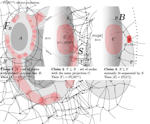
Figure 2: The $r$-projection of $u$ on $B$ (here $r=2$) is the minimal set $S\subseteq B$ which $r$-separates $u$ from $B$.

We will use the following results from [11, 13].

Lemma 19 ([11]).

Let $\mathcal{C}$ be a class of bounded expansion. Then for every $r\in\mathbb{N}$ there is a constant $c\in\mathbb{N}$ such that for every $G\in\mathcal{C}$ and $A\subseteq V(G)$ there exists a set $B$, called an $r$-closure of $A$, with the following properties:

1. $A\subseteq B\subseteq V(G)$;

2. $|B|\leqslant c\cdot|A|$; and

3. $|M_{r}^{G}(u,B)|\leqslant c$ for each $u\in V(G)$.

Moreover, for every set $X\subseteq V(G)$, it holds that

1. $|\left\{M_{r}^{G}(u,X)\,\leavevmode\nobreak\ :\leavevmode\nobreak\ \,u\in V(G)\right\}|\leqslant c\cdot|X|$.

Lemma 20 ([13]).

Let $\mathcal{C}$ be a nowhere dense class. Then for every $r\in\mathbb{N}$ and $\delta>0$ there is a constant $c\in\mathbb{N}$ such that for every $G\in\mathcal{C}$ and $A\subseteq V(G)$ there exists a set $B$, called an $r$-closure of $A$, with the following properties:

1. $A\subseteq B\subseteq V(G)$;

2. $|B|\leqslant c\cdot|A|^{1+\delta}$; and

3. $|M_{r}^{G}(u,B)|\leqslant c\cdot|A|^{\delta}$ for each $u\in V(G)$.

Moreover, for every set $X\subseteq V(G)$, it holds that

1. $|\left\{M_{r}^{G}(u,X)\,\leavevmode\nobreak\ :\leavevmode\nobreak\ \,u\in V(G)\right\}|\leqslant c\cdot|X|^{1+\delta}$.

We note that in [11, 13] projections on $B$ are defined only for vertices outside of $B$. However, adding singleton projections for vertices of $B$ to the definition only adds $|B|$ possible projections of size $1$ each, so this does not influence the validity of the above results.

We proceed with the proof of theorem 4. To focus attention, we present the proof only for the nowhere dense case (first statement). The proof in the bounded expansion case (second statement) can be obtained by replacing all the parameters $\varepsilon,\delta,\varepsilon_{1},\varepsilon_{2}$ below by $0$, and substituting the usage of lemma 20 with lemma 19.

Let us fix: a nowhere dense class of graphs $\mathcal{C}$, a graph $G\in\mathcal{C}$, a vertex subset $A\subseteq V(G)$, a real $\varepsilon>0$, and a first order formula $\varphi(\bar{x},\bar{y})$, where $\bar{x}$ is the distinguished $\ell$-tuple of object variables. Our goal is to show that $|S^{\varphi}(G/A)|=\mathcal{O}(|A|^{\ell+\varepsilon})$.

In the sequel, $d$ denotes a positive integer depending on ${\cal C},\ell,\varphi$ only (and not on $G,A$ and $\varepsilon$), and will be specified later. We may choose positive reals $\delta,\varepsilon_{1}$ such that $(\ell+\varepsilon_{1})(1+\delta)\leqslant\ell+\varepsilon$ and $\varepsilon_{1}>\delta(d+\ell)>\delta\ell$, for instance as follows: $\varepsilon_{1}=\varepsilon/2$ and $\delta=\frac{\varepsilon}{4d+4\ell}$. The constants hidden in the $\mathcal{O}(\cdot)$ notation below depend on $\varepsilon,\delta,\varepsilon_{1},\cal C,\ell$ and $\varphi$, but not on $G$ and $A$. By tuples below we refer to tuples of length $\ell$.

Let $q$ be the quantifier rank of $\varphi$ and let $p,r$ be the numbers obtained by applying lemma 15 to $q$ and $\ell$. Let $B$ be an $r$-closure of $A$, given by lemma 20. By lemma 20, the total number of distinct $r$-projections onto $B$ is at most $\mathcal{O}(|B|^{1+\delta})$, and each of these projections has size $\mathcal{O}(|B|^{\delta})$. Figure 3 serves as an illustration to the steps of the proof in the case $\ell=1$.

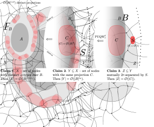
Figure 3: The proof of theorem 4 in case $\ell=1$. The logical implications flow from right to left, but our description below proceeds in the other direction.

The first step is to reduce the statement to the following claim.

Claim 1.

If $X$ is a set of tuples with pairwise different $\varphi$-types over $B$, then $|X|=\mathcal{O}(|B|^{\ell+\varepsilon_{1}})$.

1 implies that $|S^{\varphi}(G/B)|=\mathcal{O}(|B|^{\ell+\varepsilon_{1}})$, which is bounded by $\mathcal{O}(|A|^{(\ell+\varepsilon_{1})(1+\delta)})$ since $|B|=\mathcal{O}(|A|^{1+\delta})$. As $(\ell+\varepsilon_{1})(1+\delta)\leqslant\ell+\varepsilon$, this shows that $|S^{\varphi}(G/B)|=\mathcal{O}(|A|^{\ell+\varepsilon})$. Then lemma 14 implies that also $|S^{\varphi}(G/A)|=\mathcal{O}(|A|^{\ell+\varepsilon})$, and we are done. Therefore, it remains to prove 1.

For a tuple $\bar{w}=w_{1}\ldots w_{\ell}\in V(G)^{\ell}$, define its projection to be the set $C_{1}\cup\ldots\cup C_{\ell}\subseteq B$ where $C_{i}=M^{G}_{r}(w_{i},B)$. Note that there are at most $\mathcal{O}(|B|^{\ell(1+\delta)})$ different projections of tuples in total, and each projection has size $\mathcal{O}(|B|^{\delta})$. To prove 1, we consider the special case when all the tuples have the same projection, say $C\subseteq B$, and obtain a stronger conclusion, for $\varepsilon_{2}\coloneqq\varepsilon_{1}-\delta\ell>0$.

Claim 2.

If $Y$ is a set of tuples with pairwise different $\varphi$-types over $B$, and each $u\in V$ has the same projection $C\subseteq B$, then $|Y|=\mathcal{O}(|B|^{\varepsilon_{2}})$.

Since there are at most $\mathcal{O}(|B|^{\ell(1+\delta)})$ different projections in total and $\ell(1+\delta)+\varepsilon_{2}=\ell+\varepsilon_{1}$, 1 can be proved by summing the bound given by 2 through all different projections $C$. It therefore remains to prove 2.

We apply theorem 10 to the set of $\ell$-tuples $Y$, for $m$ being the largest integer such that $|Y|\geqslant N^{\ell}_{2r}(m)$. As a conclusion, we obtain a set $Z\subseteq Y$ of $m$ tuples that is mutually $2r$-separated by $S$ in $G$, for some set of vertices $S\subseteq V(G)$ of size $s\coloneqq s^{\ell}_{2r}$. Let $d$ be the degree of the polynomial $N^{\ell}_{2r}(\cdot)$ obtained from theorem 10. Note that $s=\mathcal{O}(1)$ and $|Y|=\mathcal{O}(m^{d})$.

Claim 3.

It holds that $|Z|=\mathcal{O}(|C|)$.

We first show how 3 implies 2. Since $m=|Z|=\mathcal{O}(|C|)$, and $|C|=\mathcal{O}(|B|^{\delta})$, it follows that $|Y|=\mathcal{O}(m^{d})=\mathcal{O}(|B|^{d\delta})$. As $\delta(d+\ell)>\varepsilon_{1}$, this implies that $d\delta<\varepsilon_{2}$, yielding 2. We now prove 3.

Let $Z_{0}\subseteq Z$ be the set of those tuples in $Z$ which are $r$-separated by $S$ from $B$ in $G$, and let $Z_{1}=Z-Z_{0}$ be the remaining tuples. Since tuples from $Z_{0}$ have pairwise different $\varphi$-types over $B$, and each of them is $r$-separated by $S$ from $B$ in $G$, by corollary 16 we infer that $|Z_{0}|=\mathcal{O}(1)$. On the other hand, by the definition of $Z_{1}$, with each tuple $\bar{u}\in Z_{1}$ we may associate a vertex $b(\bar{u})\in C$ which is not $r$-separated from $\bar{u}$ by $S$ in $G$. Since the set $U$ is mutually $2r$-separated by $S$ in $G$, it follows that for any two different tuples $\bar{u},\bar{v}\in Z_{1}$ we have $b(\bar{u})\neq b(\bar{v})$. Hence $b(\cdot)$ is an injection from $Z_{1}$ to $C$, which proves that $|Z_{1}|\leqslant|C|$. To conclude, we have $|Z|=|Z_{0}|+|Z_{1}|=\mathcal{O}(1)+\mathcal{O}(|C|)=\mathcal{O}(|C|)$. This finishes the proof of 3 and ends the proof of theorem 4.

6.2 Lower bounds for non-sparse classes

We now move to the proof of Theorem 5, whose statement we repeat for convenience.

Theorem 5.

Let $\mathcal{C}$ be a class of graphs which is closed under taking subgraphs.

1. If $\mathcal{C}$ is not nowhere dense, then there is a formula $\varphi(x,y)$ such that for every $n\in\mathbb{N}$ there are $G\in\mathcal{C}$ and $A\subseteq V(G)$ with $|A|=n$ and $|S^{\varphi}(G/A)|=2^{|A|}$.

2. If $\mathcal{C}$ has unbounded expansion, then there is a formula $\varphi(x,y)$ such that for every $c\in\mathbb{R}$ there exist $G\in\mathcal{C}$ and a nonempty $A\subseteq V(G)$ with $|S^{\varphi}(G/A)|>c|A|$.

Proof.

The first part follows easily from the following lemma. Let $\mathcal{G}_{r}$ be the class of $(r-1)$-subdivisions of all simple graphs, that is, the class comprising all the graphs that can be obtained from any simple graph by replacing every edge by a path of length $r$.

Lemma 21 ([28]).

For every somewhere dense graph class $\mathcal{C}$ that is closed under taking subgraphs, there exists a positive integer $r$ such that $\mathcal{G}_{r}\subseteq\mathcal{C}$.

To prove the first statement of Theorem 5, for $n\in\mathbb{N}$, let $P(n)$ denote the graph with $n+2^{n}$ vertices $V(P(n))\coloneqq\{v_{1},\ldots,v_{n}\}\cup\{w_{M}\colon M\subseteq\{1,\ldots,n\}\}$ and edges $E(P(n))\coloneqq\{v_{i}w_{M}\colon 1\leqslant i\leqslant n,\,M\subseteq\{1,\ldots,n\},\,i\in M\}$. If $\mathcal{C}$ is somewhere dense and closed under taking subgraphs, according to Lemma 21, there exists an integer $r$ such that $\mathcal{G}_{r}\subseteq\mathcal{C}$. In particular, for every $n\in\mathbb{N}$ the $(r-1)$-subdivision $P^{r}(n)$ of the graph $P(n)$ is contained in $\mathcal{C}$. Now consider the formula $\varphi(x,y)$ stating that $x$ and $y$ are at distance at most $r$. Then for every $n\in\mathbb{N}$ we have $S^{\varphi}(P^{r}(n)/A)=\mathcal{P}(A)$, where $A\subseteq V(P^{r}(n))$ denotes the set $\{v_{1},\ldots,v_{n}\}$. This implies the first part of the theorem.

We now move to the second part of theorem 5. A graph $H$ is a topological depth-$r$ minor of $G$ if there is a mapping $\varphi$ that maps vertices of $H$ to vertices of $G$ such that $\varphi(u)\neq\varphi(v)$ for $u\neq v$, and edges of $H$ to paths in $G$ such that if $uv\in E(H)$, then $\varphi(uv)$ is a path of length at most $2r+1$ between $u$ and $v$ in $G$ and furthermore, if $uv,xy\in E(H)$, then $\varphi(uv)$ and $\varphi(xy)$ are internally vertex disjoint. We write $H\preccurlyeq_{r}^{\mathrm{t}}G$. Note that the above definition makes sense for half-integers, i.e., numbers $r$ for which $2r$ is an integer.

It is well-known that classes of bounded expansion can be alternatively characterized by the sparsity of shallow topological minors.

Lemma 22 (Corollary 4.1 of [29]).

A class $\mathcal{C}$ of graphs has bounded expansion if and only if for every $r\in\mathbb{N}$ there exists a constant $c_{r}$ such that $|E(H)|/|V(H)|\leqslant c_{r}$ for all graphs $H$ such that $H\preccurlyeq_{r}^{\mathrm{t}}G$ for some $G\in\mathcal{C}$.

For $r\in\mathbb{N}$ and a graph $G$, by $\nu_{r}(G)$ we denoted the normed $r$-neighborhood complexity of $G$, as defined by Reidl et al. [32]:

$$\nu_{r}(G)\coloneqq\max_{H\subseteq G,\,\emptyset\neq A\subseteq V(G)}\frac{|\{N_{r}^{H}[v]\cap A\,\colon\,v\in V(H)\}|}{|A|}.$$

We will need the following result relating edge density in shallow topological minors and normed neighborhood complexity.

Lemma 23 (Theorem 4 of [32]).

Let $G$ be a graph, $r$ be a half-integer, and let $H\preccurlyeq_{r}^{\mathrm{t}}G$. Then

$$\frac{|E(H)|}{|V(H)|}\leqslant(2r+1)\cdot\max\left\{\nu_{1}(G)^{4}\cdot\log^{2}\nu_{1}(G),\nu_{2}(G),\ldots,\nu_{\left\lceil r+\frac{1}{2}\right\rceil}(G)\right\}.$$

For the second part of theorem 5, we use the contrapositive of Lemma 22. Since $\mathcal{C}$ has unbounded expansion, for some $r\in\mathbb{N}$ we have that the value $|E(H)|/|V(H)|$ is unbounded among depth-$r$ topological minors $H$ of graphs from $\mathcal{C}$. By applying Lemma 23, we find that for some $q\leqslant r$ the value $\nu_{q}(G)$ is unbounded when $G$ ranges over all graphs from $\mathcal{C}$. Since $\mathcal{C}$ is closed under taking subgraph, we infer that also the ratio $\frac{|\{N_{q}^{G}[v]\cap A\colon v\in V(G)\}|}{|A|}$ is unbounded when $G$ ranges over graphs from $\mathcal{C}$ and $A$ ranges over nonempty subsets of $V(G)$. This is equivalent to the sought assertion for the formula $\varphi(x,y)$ expressing that $x$ and $y$ are at distance at most $q$.

$\square$

7 Packing and traversal numbers for nowhere dense graphs

In this section, we give an application of theorem 4, proving a duality result for nowhere dense graph classes.

A set system is a family $\cal F$ of subsets of a set $X$. Its packing is a subfamily of $\cal F$ of pairwise disjoint subsets, and its traversal (or hitting set) is a subset of $X$ which intersects every member of $\cal F$. The packing number of $\cal F$, denoted $\nu(\cal F)$, is the largest cardinality of a packing in $\cal F$, and the transversality of $\cal F$, denoted $\tau(\cal F)$, is the smallest cardinality of a traversal of $\cal F$. Note that if $\cal G$ is a finite set system, then $\nu({\cal G})\leqslant\tau(\cal G)$. The set system $\cal F$ has the Erdős-Pósa property if there is a function $f\colon\mathbb{N}\to\mathbb{N}$ such that every finite subfamily $\cal G$ of $\cal F$ satisfies $\tau({\cal G})\leqslant f(\nu(\cal G))$.

We prove that set systems defined by first order formulas in nowhere dense graph classes have the Erdős-Pósa property, in the following sense.

Theorem 7.

Fix a nowhere dense class of graphs $\mathcal{C}$ and a formula $\varphi(x,y)$ with two free variables $x,y$. Then there is a function $f\colon\mathbb{N}\to\mathbb{N}$ with the following property. Let $G\in\mathcal{C}$ be a graph and let $\cal G$ be a family of subsets of $V(G)$ consisting of sets of the form $\left\{v\in V(G)\,\leavevmode\nobreak\ :\leavevmode\nobreak\ \,\varphi(u,v)\right\}$, where $u$ is some vertex of $V(G)$. Then $\tau({\cal G})\leqslant f(\nu(\cal G))$.

We will apply the following result of Matoušek [25], which relies on the proof of Alon and Kleitman [2] of the conjecture of Hardwiger and Debrunner. In the result of Matoušek, the set system $\cal F$ is infinite. For $m\in\mathbb{N}$, by $\pi_{\cal F}^{*}(m)$ we denote the dual shatter function of $\cal F$, which is defined as the maximal number of occupied cells in the Venn diagram of $m$ sets in $\cal F$.

Theorem 11 (Matoušek, [25]).

Let $\cal F$ be a set system with $\pi^{*}_{\cal F}(m)=o(m^{k})$, for some integer $k$, and let $p\geqslant k$. Then there is a constant $T$ such that the following holds for every finite family $\cal G\subseteq\cal F$: if $\cal G$ has the $(p,k)$-property, meaning that among every $p$ sets in $\cal G$ some $k$ have a non-empty intersection, then $\tau({\cal G})\leqslant T$.

Proof (of theorem 7).

For a graph $G$, define the set system ${\cal F}_{G}$ on the ground set $V(G)$ as

$${\cal F}_{G}=\left\{\left\{v\in V(G)\,\leavevmode\nobreak\ :\leavevmode\nobreak\ \,\varphi(u,v)\right\}\,\leavevmode\nobreak\ :\leavevmode\nobreak\ \,u\in V(G)\right\}.$$

Let then $\cal F$ be the disjoint union of set systems ${\cal F}_{G}$ for $G\in\mathcal{C}$. That is, the ground set of $\cal F$ is the disjoint union of the vertex sets $V(G)$ for $G\in\mathcal{C}$, and for each $G\in\mathcal{C}$ we add to ${\cal F}$ a copy of ${\cal F}_{G}$ over the copy of relevant $V(G)$. Then the following claim follows directly from theorem 4.

Claim 4.

The dual shatter function of $\cal F$ satisfies $\pi^{*}_{\cal F}(m)=\mathcal{O}(m^{1+\varepsilon})$, for every fixed $\varepsilon>0$. In particular, $\pi^{*}_{\cal F}(m)=o(m^{2})$.

Consider the function $f\colon\mathbb{N}\to\mathbb{N}$ defined so that $f(\nu)$ is the value $T$ obtained from theorem 11 applied to $\cal F$, $k=2$, and $p=\nu+1$. Suppose now that $G\in\mathcal{C}$ is a graph and $\mathcal{G}\subseteq\mathcal{F}_{G}$ is a family of subsets of $V(G)$ consisting of sets of the form $\{v\in V(G)\,\colon\,\varphi(u,v)\}$, where $u$ is some vertex of $G$. We identify $\mathcal{G}$ with a subfamily of $\mathcal{F}$ in the natural way, following the embedding of $\mathcal{F}_{G}$ into $\mathcal{F}$ used in the construction of the latter. Let $\nu$ be the packing number of $\mathcal{G}$. In particular, for every $\nu+1$ subsets of $\mathcal{G}$ there is a vertex $v\in V(G)$ which is contained in two elements of $\mathcal{G}$. Hence, $\mathcal{G}$ is a $(p,2)$-family for $p=\nu+1$. By theorem 11, $\tau(\mathcal{G})\leqslant T=f(\nu)=f(\nu(\mathcal{G}))$, as required. $\square$

8 Bounds for stability

As mentioned, Adler and Adler [1], proved that every nowhere dense class of graphs is stable. In this section, we prove its effective variant, theorem 8, which we repeat for convenience.

Theorem 8.

There are computable functions $f\colon\mathbb{N}^{3}\to\mathbb{N}$ and $g\colon\mathbb{N}\to\mathbb{N}$ with the following property. Suppose $\varphi(\bar{x},\bar{y})$ is a formula of quantifier rank at most $q$ and with $d$ free variables. Suppose further that $G$ is a graph excluding $K_{t}$ as a depth-$g(q)$ minor. Then the ladder index of $\varphi(\bar{x},\bar{y})$ in $G$ is at most $f(q,d,t)$.

Recall that a class $\cal C$ is stable if and only if for every first order formula $\varphi(\bar{x},\bar{y})$, its ladder index over graphs from $\cal C$ is bounded by a constant depending only on $\cal C$ and $\varphi$; see section 1 to recall the background on stability. Thus the result of Adler and Adler is implied by theorem 8, and is weaker in the following sense: theorem 8 asserts in addition that there is a computable bounds on the ladder index of any formula that depends only on the size of an excluded clique minor at depth bounded in terms of formula’s quantifier rank and number of free variables. We now prove theorem 8.

Proof (of theorem 8).

Fix a formula $\varphi(\bar{x},\bar{y})$ of quantifier rank $q$ and a partitioning of its free variables into $\bar{y}$ and $\bar{z}$. Let $d=|\bar{x}|+|\bar{y}|$ be the total number of free variables of $\varphi$. Let $r\in\mathbb{N}$ be the number given by corollary 16, which depends on $\varphi$ only. Let $\cal C$ be the class of all graphs such that $K_{t}\not\preccurlyeq_{18r}G$. Then, by theorem 10, $\cal C$ satisfies $\mathrm{UQW}^{d}_{r}(N^{d}_{r},s^{d}_{r})$, for some polynomial $N^{d}_{r}\colon\mathbb{N}\to\mathbb{N}$ and number $s=s^{d}_{r}\in\mathbb{N}$ computable from $d,t,r$. Let $T$ be the number given by corollary 16 for $\varphi$ and $s$. Finally, let $\ell=N^{d}_{r}(2T+1)$. We show that every $\varphi$-ladder in a graph $G\in\cal C$ has length smaller than $\ell$.

For the sake of contradiction, assume that there is a graph $G\in\cal C$ and tuples $\bar{u}_{1},\ldots,\bar{u}_{\ell}\in V(G)^{|\bar{x}|}$ and $\bar{v}_{1},\ldots,\bar{v}_{\ell}\in V(G)^{|\bar{y}|}$ which form a $\varphi$-ladder in $G$, i.e., $\varphi(\bar{u}_{i},\bar{v}_{j})$ holds in $G$ if and only if $i\leqslant j$. Let $A=\left\{\bar{u}_{i}\bar{v}_{i}\,\leavevmode\nobreak\ :\leavevmode\nobreak\ \,i=1,\ldots,\ell\right\}\subseteq V(G)^{d}$. Note that $|A|=\ell\geqslant N^{d}_{r}(2T+1)$, since tuples $\bar{u}_{i}$ have to be pairwise different.

Applying property $\mathrm{UQW}^{d}_{r}(N^{d}_{r},s^{d}_{r})$ to the set $A$, radius $r$, and target size $m=2T+1$ yields a set $S\subseteq V(G)$ with $|S|\leqslant s$ and a set $B\subseteq A$ with $|B|\geqslant 2T+1$ of tuples which are mutually $r$-separated by $S$ in $G$. Let $J\subseteq\{1,\ldots,\ell\}$ be the set of indices corresponding to $B$, i.e., $J=\{j\colon\bar{u}_{j}\bar{v}_{j}\in B\}$.

Since $|J|=2T+1$, we may partition $J$ into $J_{1}\uplus J_{2}$ with $|J_{1}|=T+1$ so that the following condition holds: for each $i,k\in J_{1}$ satisfying $i<k$, there exists $j\in J_{2}$ with $i<j<k$. Indeed, it suffices to order the indices of $J$ and put every second index to $J_{1}$, and every other to $J_{2}$. Let $X$ be the set of vertices appearing in the tuples $\bar{u}_{i}$ with $i\in J_{1}$, and let $Y$ be the set of vertices appearing in the tuples $\bar{v}_{j}$ with $j\in J_{2}$. Since the tuples of $B$ are mutually $r$-separated by $S$ in $G$, it follows that $X$ and $Y$ are $r$-separated by $S$. As $|J_{1}|=T+1$, by corollary 16 we infer that there are distinct indices $i,k\in J_{1}$, say $i<k$, such that $\mathrm{tp}^{\varphi}(\bar{u}_{i}/Y)=\mathrm{tp}^{\varphi}(\bar{u}_{k}/Y)$. This implies that for each $j\in J_{2}$, we have $G,\bar{u}_{i},\bar{v}_{j}\models\varphi(\bar{x},\bar{y})$ if and only if $G,\bar{u}_{k},\bar{v}_{j}\models\varphi(\bar{x},\bar{y})$. However, there is an index $j\in J_{2}$ such that $i<j<k$, and for this index we should have $G,\bar{u}_{i},\bar{v}_{j}\models\varphi(\bar{x},\bar{y})$ and $G,\bar{u}_{k},\bar{v}_{j}\not\models\varphi(\bar{x},\bar{y})$ by the definition of a ladder. This contradiction concludes the proof. $\square$

We remark that theorem 8 also holds for classes of edge- and vertex-colored graphs, with the same proof, but using a version of the results in section 5 lifted to edge- and vertex-colored graphs.

References

- [1] H. Adler and I. Adler. Interpreting nowhere dense graph classes as a classical notion of model theory. European Journal of Combinatorics, 36:322–330, 2014.
- [2] N. Alon and D. J. Kleitman. Piercing convex sets and the hadwiger-debrunner (p, q)-problem. Advances in Mathematics, 96(1):103 – 112, 1992.
- [3] N. Alon, M. Krivelevich, and B. Sudakov. Turán numbers of bipartite graphs and related Ramsey-type questions. Combinatorics, Probability and Computing, 12(5+ 6):477–494, 2003.
- [4] M. Aschenbrenner, A. Dolich, D. Haskell, D. Macpherson, and S. Starchenko. Vapnik-Chervonenkis density in some theories without the independence property, I. Transactions of the American Mathematical Society, 368(8):5889–5949, 2016.
- [5] A. Atserias, A. Dawar, and P. G. Kolaitis. On preservation under homomorphisms and unions of conjunctive queries. Journal of the ACM (JACM), 53(2):208–237, 2006.
- [6] N. Bousquet and S. Thomassé. VC-dimension and Erdős-Pósa property. Discrete Mathematics, 338(12):2302–2317, 2015.
- [7] H. Brönnimann and M. T. Goodrich. Almost optimal set covers in finite VC-dimension. Discrete & Computational Geometry, 14(4):463–479, 1995.
- [8] A. Chervonenkis and V. Vapnik. Theory of uniform convergence of frequencies of events to their probabilities and problems of search for an optimal solution from empirical data. Automation and Remote Control, 32:207–217, 1971.
- [9] A. Dawar. Homomorphism preservation on quasi-wide classes. Journal of Computer and System Sciences, 76(5):324–332, 2010.
- [10] R. Diestel. Graph Theory, 4th Edition, volume 173 of Graduate Texts in Mathematics. Springer, 2012.
- [11] P. G. Drange, M. S. Dregi, F. V. Fomin, S. Kreutzer, D. Lokshtanov, M. Pilipczuk, M. Pilipczuk, F. Reidl, F. Sánchez Villaamil, S. Saurabh, S. Siebertz, and S. Sikdar. Kernelization and sparseness: the case of Dominating Set. In STACS 2016, volume 47 of LIPIcs, pages 31:1–31:14. Schloss Dagstuhl—Leibniz-Zentrum für Informatik, 2016. See \urlhttps://arxiv.org/abs/1411.4575 for full proofs.
- [12] Z. Dvořák, D. Král, and R. Thomas. Testing first-order properties for subclasses of sparse graphs. Journal of the ACM (JACM), 60(5):36, 2013.
- [13] K. Eickmeyer, A. C. Giannopoulou, S. Kreutzer, O. Kwon, M. Pilipczuk, R. Rabinovich, and S. Siebertz. Neighborhood complexity and kernelization for nowhere dense classes of graphs. In ICALP 2017, volume 80 of LIPIcs, pages 63:1–63:14. Schloss Dagstuhl—Leibniz-Zentrum für Informatik, 2017. See \urlhttps://arxiv.org/abs/1612.08197 for full proofs.
- [14] Z. Füredi and J. Pach. Traces of finite sets: extremal problems and geometric applications. Extremal problems for finite sets, 3:255–282, 1991.
- [15] H. Gaifman. On local and non-local properties. Studies in Logic and the Foundations of Mathematics, 107:105–135, 1982.
- [16] M. Grohe and S. Kreutzer. Methods for algorithmic meta theorems. In M. Grohe and J. Makowsky, editors, Model Theoretic Methods in Finite Combinatorics, volume 558 of Contemporary Mathematics, pages 181–206. American Mathematical Society, 2011.
- [17] M. Grohe, S. Kreutzer, R. Rabinovich, S. Siebertz, and K. Stavropoulos. Colouring and covering nowhere dense graphs. In WG 2015, volume 9224 of Lecture Notes in Computer Science, pages 325–338. Springer, 2015.
- [18] M. Grohe, S. Kreutzer, and S. Siebertz. Deciding first-order properties of nowhere dense graphs. In STOC 2014, pages 89–98. ACM, 2014.
- [19] A. A. Ivanov. The structure of superflat graphs. Fundamenta Mathematicae, 143:107–117, 1993.
- [20] M. Kreidler and D. Seese. Monadic NP and graph minors. In CSL 1998, volume 1584 of Lecture Notes in Computer Science, pages 126–141. Springer, 1998.
- [21] S. Kreutzer, R. Rabinovich, and S. Siebertz. Polynomial kernels and wideness properties of nowhere dense graph classes. In SODA 2017, pages 1533–1545. SIAM, 2017.
- [22] M. C. Laskowski. Vapnik-Chervonenkis classes of definable sets. Journal of the London Mathematical Society, 2(2):377–384, 1992.
- [23] M. Malliaris and S. Shelah. Regularity lemmas for stable graphs. Transactions of the American Mathematical Society, 366(3):1551–1585, 2014.
- [24] J. Matoušek. Geometric set systems. In European Congress of Mathematics, volume 2, page 23. Birkhäuser, Basel, 1998.
- [25] J. Matoušek. Bounded VC-dimension implies a fractional Helly theorem. Discrete & Computational Geometry, 31(2):251–255, 2004.
- [26] J. Nešetřil and P. Ossona de Mendez. Grad and classes with bounded expansion I. Decompositions. European Journal of Combinatorics, 29(3):760–776, 2008.
- [27] J. Nešetřil and P. Ossona de Mendez. First order properties on nowhere dense structures. The Journal of Symbolic Logic, 75(03):868–887, 2010.
- [28] J. Nešetřil and P. Ossona de Mendez. On nowhere dense graphs. European Journal of Combinatorics, 32(4):600–617, 2011.
- [29] J. Nešetřil and P. Ossona de Mendez. Sparsity — Graphs, Structures, and Algorithms, volume 28 of Algorithms and combinatorics. Springer, 2012.
- [30] A. Pillay. Introduction to Stability Theory. Dover Books on Mathematics. Dover Publications, 2008.
- [31] K.-P. Podewski and M. Ziegler. Stable graphs. Fundamenta Mathematicae, 100(2):101–107, 1978.
- [32] F. Reidl, F. Sánchez Villaamil, and K. Stavropoulos. Characterising bounded expansion by neighbourhood complexity. CoRR, abs/1603.09532, 2016.
- [33] N. Sauer. On the density of families of sets. Journal of Combinatorial Theory, Series A, 13(1):145–147, 1972.
- [34] S. Shelah. A combinatorial problem; stability and order for models and theories in infinitary languages. Pacific Journal of Mathematics, 41(1):247–261, 1972.
- [35] S. Shelah. Classification theory: and the number of non-isomorphic models, volume 92 of Studies in Logic and the Foundations of Mathematics. Elsevier, 1990.
- [36] K. Tent and M. Ziegler. A Course in Model Theory. Lecture Notes in Logic. Cambridge University Press, 2012.
- [37] X. Zhu. Colouring graphs with bounded generalized colouring number. Discrete Mathematics, 309(18):5562–5568, 2009.