Smoothing Method for Approximate Extensive-Form Perfect Equilibrium

Abstract

Nash equilibrium is a popular solution concept for solving imperfect-information games in practice. However, it has a major drawback: it does not preclude suboptimal play in branches of the game tree that are not reached in equilibrium. Equilibrium refinements can mend this issue, but have experienced little practical adoption. This is largely due to a lack of scalable algorithms.

Sparse iterative methods, in particular first-order methods, are known to be among the most effective algorithms for computing Nash equilibria in large-scale two-player zero-sum extensive-form games. In this paper, we provide, to our knowledge, the first extension of these methods to equilibrium refinements. We develop a smoothing approach for behavioral perturbations of the convex polytope that encompasses the strategy spaces of players in an extensive-form game. This enables one to compute an approximate variant of extensive-form perfect equilibria. Experiments show that our smoothing approach leads to solutions with dramatically stronger strategies at information sets that are reached with low probability in approximate Nash equilibria, while retaining the overall convergence rate associated with fast algorithms for Nash equilibrium. This has benefits both in approximate equilibrium finding (such approximation is necessary in practice in large games) where some probabilities are low while possibly heading toward zero in the limit, and exact equilibrium computation where the low probabilities are actually zero.

1 Introduction

Nash equilibrium is the basic solution concept for noncooperative games, including extensive-form games (EFGs), a broad class of games that model sequential and simultaneous interaction, imperfect information, and outcome uncertainty Sandholm (2010); Bowling et al. (2015); Brown et al. (2015); Moravčík et al. (2017). Nash equilibrium was the solution concept used in the Libratus agent, which showed superhuman performance against a team of top Heads-Up No-Limit Texas hold’em poker specialist professional players in the Brains vs. AI event in January 2017 Brown and Sandholm (2017a). It was also used in the DeepStack agent Moravčík et al. (2017), which beat a group of professional players. It has also been dominant in the Annual Computer Poker Competition [ACPC], where the winning agents have all been based on Nash equilibrium approximation for many years.

In spite of this popularity, Nash equilibria suffer from a major deficiency: they might not play reasonably in parts of the game tree that are reached with zero probability in equilibrium. In particular, the only guarantee that Nash equilibrium gives in these parts of the game tree is that it does not give up more utility than the value of the game. Thus, if the opponent makes a big mistake, Nash equilibrium might give back all the utility gained from the opponent making that mistake, since it is only maintaining the value of the game (Miltersen and Sørensen Miltersen and Sørensen (2010) show nice examples of such behavior).

The above shows that Nash equilibrium is not satisfactory in extensive-form games, and is the motivation for equilibrium refinements Selten (1975). When information is perfect, the classical solution concept of subgame-perfect equilibrium (SPE) can be satisfactory, while it is not when information is imperfect. In this latter case, refinements are usually based on the idea of perturbations representing mistakes of the players. In a quasi-perfect equilibrium (QPE) van Damme (1984), a player maximizes her utility in each decision node taking into account the future mistakes of the opponents only, whereas, in an extensive-form perfect equilibrium (EFPE), players maximize their utility in each decision node taking into account the future mistakes of both themselves and their opponents Selten (1975); Hillas and Kohlberg (2002).

Computation of Nash equilibrium refinements in EFGs has received some attention in the literature. Von Stengel et. al. von Stengel et al. (2002) give a pivoting algorithm for computing normal-form-perfect equilibria in EFGs. Miltersen and Sørensen Miltersen and Sørensen (2010) give an algorithm for computing quasi-perfect equilibria. Miltersen and Sørensen Miltersen and Sørensen (2008) show how to compute a normal-form-proper equilibrium. Farina and Gatti Farina and Gatti (2017) give an algorithm for computing extensive-form perfect equilibria. All these results rely on linear programming (LP) (in the zero-sum case) or linear complementary programming (LCP). In zero-sum games, several of these solution concepts can be computed in polynomial time using an LP or a series of LPs. However, even for the easier case of Nash equilibria, the LP approach is not scalable for large games (beyond roughly $10^{8}$ nodes in the game tree Gilpin and Sandholm (2007)). Each iteration of an LP-solving algorithm is expensive, and the LP might even be too large to fit in memory. In practice, iterative methods are preferred, even for games of modest size. These methods have iteration costs that are usually linear, or better, in the game size, but converge to a Nash equilibrium only in the limit. The most prominent of these methods are counterfactual regret minimization (CFR) Zinkevich et al. (2007) and its variants Lanctot et al. (2009); Tammelin et al. (2015); Brown and Sandholm (2015); Brown and Sandholm (2017b), and general first-order methods (FOMs) such as the excessive gap technique (EGT) Nesterov (2005a) instantiated with an appropriate EFG smoothing technique Hoda et al. (2010); Kroer et al. (2015, 2017). Farina et al. Farina et al. (2017) show how to extend CFR to approximate EFPEs.

In this paper, we show how to extend FOMs to the computation of an approximate variant of EFPE. Miltersen and Sørensen Miltersen and Sørensen (2010) and Farina and Gatti Farina and Gatti (2017) presented perturbed polytopes of EFGs that capture equilibrium refinements where each action has to be played with positive probability. We prove that recent results on smoothing techniques for EFGs based on dilating the entropy function can be modified to provide smoothing for such perturbed games, where the perturbations are with respect to behavioral strategies. We then instantiate this method for the perturbed game of Farina and Gatti, which leads to our approximate EFPE.

We then experimentally validate our method. We show that it is effective at obtaining low maximum regret at each information set of the game—even ones that have low probability of being reached—while simultaneously achieving the same practical convergence rate that FOMs and the best CFR variants traditionally achieve for just Nash equilibrium. This has benefits both in approximate Nash equilibrium finding (such approximation is necessary in practice in large games) where some probabilities are low while possibly heading toward zero in the limit, and exact Nash equilibrium computation where the low probabilities are actually zero.

2 Preliminaries

We assume that the reader is familiar with the classical concept of extensive-form game. We invite the reader unfamiliar with the topic to refer to Shoham and Leyton-Brown Shoham and Leyton-Brown (2008) or any classic textbook on the subject for further information and context. Briefly, an extensive-form game $\Gamma$ is defined over a game tree. In each non-terminal node a single player moves and each edge corresponds to an action available to the player. Each leaf node is associated with a payoff vector, representing the utility for the two players when the game finishes in the leaf.

A Nash equilibrium is defined in Definition 2.

Definition 1.

An $\epsilon$-NE is a strategy profile $(\pi_{1},\pi_{2})$ for the players, such that no player can gain more than $\epsilon$ by unilaterally deviating from their strategy.

Definition 2.

A Nash equilibrium (NE) is a 0-NE.

However, Nash equilibria might not be satisfactory when dealing with EFGs, independently of whether the game has perfect or imperfect information, and whether it is general- or zero-sum. A Nash equilibrium $\pi$ might prescribe irrational play in those information sets that are visited with zero probability when playing according to $\pi$ (e.g., Miltersen and Sørensen (2008)). In the general-sum case, consider the left example of Figure 1: the strategy profile $(\pi_{1},\pi_{2})$ where player 1 always chooses action x and player 2 always chooses action y is a NE. However, this strategy profile is irrational: Player 2 is “threatening” to play a suboptimal action, and Player 1 is caving in to the threat. Yet, the threat is not credible: if Player 1 were to actually play action y, it would be irrational for Player 2 to honor the threat.

Figure 1: General-sum (left) and zero-sum (right) games where Nash equilibrium prescribes irrational play. Numbers in parentheses denote the payoffs to Players 1 and 2.

The right example in Figure 1 shows that even in zero-sum games, a NE can fail to capture (sequential) rationality. In this game, the same strategy profile as in the previous game is again a NE. If Player 2 plays according to this profile, she gives up a potential payoff of 5 if Player 1 plays action y.

2.1 Perturbations and Extensive-Form Perfection

A way to mend the issue just described is to introduce the idea of “trembling hands”: each player cannot fully commit to a pure strategy, and ends up making mistakes with a small (yet strictly positive) probability. This guarantees that the whole game tree gets visited. More formally, let $l(h,a)$ be the perturbation of the game, a (positive) function defining the minimum amount of probability mass with which the player playing at information set $h$ in the game will select action $a$ when playing in $h$. Let $\Gamma_{l}$ be the game where players are subject to such perturbation: an extensive-form perfect equilibrium of the game $\Gamma$ is any limit point of the sequence of Nash equilibria of the game $\Gamma_{l}$, as $l$ vanishes Selten (1975). In this paper, we deal with the simplest form of perturbation – a uniform perturbation $l_{\xi}$ for ${\xi}>0$, defined as $l_{{\xi}}(h,a)={\xi}$ for all $a$ and $h$. We will denote the game $\Gamma_{l_{\xi}}$ as $\Gamma_{\xi}$.

2.2 Bilinear Saddle-Point Problems and the Sequence Form

It is well-known that the strategy spaces of an extensive-form game can be transformed into convex polytopes that allow a bilinear saddle-point formulation (BSPP) of the Nash equilibrium problem as follows Romanovskii (1962); von Stengel (1996); Koller et al. (1996).

$$\min_{x\in{\cal X}}\max_{y\in{\cal Y}}\langle x,Ay\rangle=\max_{y\in{\cal Y}}\min_{x\in{\cal X}}\langle x,Ay\rangle$$ (1)

Our approach for computing equilibrium refinements will be based on constructing a perturbed variant of ${\cal X}$ and ${\cal Y}$.

Several FOMs with attractive convergence properties have been introduced for BSPPs Nesterov (2005b, a); Nemirovski (2004); Chambolle and Pock (2011). These methods rely on having some appropriate distance measure over ${\cal X}$ and ${\cal Y}$, called a distance-generating function (DGF). Generally, FOMs use the DGF to choose steps: given a gradient and a scalar stepsize, a FOM moves in the negative gradient direction by finding the point that minimizes the sum of the gradient and of the DGF evaluated at the new point. In other words, the next step can be found by solving a regularized optimization problem, where long gradient steps are discouraged by the DGF. For EGT on EFGs, the DGF can be interpreted as a smoothing function applied to the best-response problems faced by the players.

Definition 3.

A distance-generating function for ${\cal X}$ is a function $d(x):{\cal X}\rightarrow{\mathbb{R}}$ which is convex and continuous on ${\cal X}$, admits continuous selection of subgradients on the set ${\cal X}^{\circ}=\left\{x\in{\cal X}:\partial d(x)\neq\emptyset\right\}$, and is strongly convex modulus $\varphi$ w.r.t. $\|\cdot\|$. Distance-generating functions for ${\cal Y}$ are defined analogously.

Given a twice differentiable function $f$, we let $\nabla^{2}f(z)$ denote its Hessian at $z$. Our analysis is based on the following sufficient condition for strong convexity of a twice differentiable function:

Fact 1.

A twice-differentiable function $f$ is strongly convex with modulus $\varphi$ with respect to a norm $\|\cdot\|$ on nonempty convex set $C\subset{\mathbb{R}}^{n}$ if $h^{\top}\nabla^{2}f(z)h\geq\varphi\|h\|,\ \forall h\in{\mathbb{R}}^{n},z\in C^{\circ}.$

Given DGFs $d_{{\cal X}},d_{{\cal Y}}$ for ${\cal X},{\cal Y}$ with strong convexity moduli $\varphi_{{\cal X}}$ and $\varphi_{{\cal Y}}$ respectively, we now describe the Excessive Gap Technique (EGT) Nesterov (2005a) applied to (1). EGT forms two smoothed functions using the DGFs

$$\vspace{-1mm}f_{\mu_{y}}(x)=\max_{y\in{\cal Y}}\langle x,Ay\rangle-\mu_{\cal Y}d_{\cal Y},$$ (2)

$$\phi_{\mu_{x}}(y)=\min_{x\in{\cal X}}\langle x,Ay\rangle+\mu_{\cal X}d_{\cal X}.\vspace{-1mm}$$ (3)

These functions are smoothed approximations to the optimization problem faced by the $x$ and $y$ player, respectively. The scalars $\mu_{1},\mu_{2}>0$ are smoothness parameters denoting the amount of smoothing applied. Let $y_{\mu_{2}}(x)$ and $x_{\mu_{1}}(y)$ refer to the $y$ and $x$ values attaining the optima in (2) and (3). These can be thought of as smoothed best responses. Nesterov Nesterov (2005b) shows that the gradients of the functions $f_{\mu_{2}}(x)$ and $\phi_{\mu_{1}}(y)$ exist and are Lipschitz continuous. The gradient operators and Lipschitz constants are given as follows

$\displaystyle\nabla f_{\mu_{2}}(x)=a_{1}+Ay_{\mu_{2}}(x),\quad\nabla\phi_{\mu_{1}}(y)=a_{2}+A^{\top}x_{\mu_{1}}(y),$ $\displaystyle L_{1}\left(f_{\mu_{2}}\right)=\frac{\|A\|^{2}}{\varphi_{\cal Y}\mu_{2}}$ and $\displaystyle L_{2}\left(\phi_{\mu_{1}}\right)=\frac{\|A\|^{2}}{\varphi_{\cal X}\mu_{1}}$.

Let the convex conjugate of $d:Q\rightarrow{\mathbb{R}}$ be denoted by $d^{*}(q)=\max_{q\in Q}g^{T}q-d(q)$. Based on this setup, we formally state EGT Nesterov (2005a) as Algorithm 1.

The EGT algorithm alternates between taking steps focused on ${\cal X}$ and ${\cal Y}$. Algorithm 2 shows a single step focused on ${\cal X}$. Steps focused on $y$ are analogous. Algorithm 1 shows how the alternating steps and stepsizes are computed, as well as how initial points are selected.

Suppose the initial values $\mu_{1},\mu_{2}$ satisfy $\mu_{1}=\frac{\varphi_{\cal X}}{L_{1}(f_{\mu_{2}})}$. Then, at every iteration $t\geq 1$ of EGT, the corresponding solution $z^{t}=[x^{t};y^{t}]$ satisfies $x^{t}\in{\cal X}$, $y^{t}\in{\cal Y}$, and

$$\vspace{-1mm}\max_{y\in{\cal Y}}(x^{t})^{T}Ay-\min_{x\in{\cal X}}x^{T}Ay^{t}={\epsilon_{\hbox{\scriptsize\rm sad}}}(z^{t})\leq\frac{4\|A\|}{T+1}\sqrt{\frac{\Omega_{\cal X}\Omega_{\cal Y}}{\varphi_{\cal X}\varphi_{\cal Y}}}.\vspace{-1mm}$$

Consequently, EGT has a convergence rate of $O(\frac{1}{\epsilon})$ Nesterov (2005a).

2.3 Treeplexes

Hoda et al. Hoda et al. (2010) introduce the treeplex, a class of convex polytopes that captures the sequence-form of the strategy spaces in perfect-recall EFGs.

Definition 4.

Treeplexes are defined recursively:

1. Basic sets: The standard simplex $\Delta_{m}$ is a treeplex.

2. Cartesian product: If $Q_{1},\ldots,Q_{k}$ are treeplexes, then $Q_{1}\times\cdots\times Q_{k}$ is a treeplex.

3. Branching: Given a treeplex $P\subseteq\left[0,1\right]^{p}$, a collection of treeplexes $Q=\left\{Q_{1},\ldots,Q_{k}\right\}$ where $Q_{j}\subseteq\left[0,1\right]^{n_{j}}$, and $l=\left\{l_{1},\ldots,l_{k}\right\}\subseteq\left\{1,\ldots,p\right\}$, the set defined by

   $$\vspace{-1mm}P\framebox{l}Q\coloneqq\left\{\left(x,y_{1},\ldots,y_{k}\right)\in{\mathbb{R}}^{p+\sum_{j}n_{j}}:~{}x\in P,\right.$$

   $$\left.\,y_{1}\in x_{l_{1}}\cdot Q_{1},\,\ldots,y_{k}\in x_{l_{k}}\cdot Q_{k}\vphantom{{\mathbb{R}}^{\sum}}\right\}\vspace{-1mm}$$

   is a treeplex. We say $x_{l_{j}}$ is the branching variable for the treeplex $Q_{j}$.

For a treeplex $Q$, we denote by $S_{Q}$ the index set of the set of simplexes contained in $Q$ (in an EFG $S_{Q}$ is the set of information sets belonging to the player). For each $j\in S_{Q}$, the treeplex rooted at the $j$-th simplex $\Delta^{j}$ is referred to as $Q_{j}$. Given vector $q\in Q$ and simplex $\Delta^{j}$, we let $\mathbb{I}_{j}$ denote the set of indices of $q$ that correspond to the variables in $\Delta^{j}$ and define $q^{j}$ to be the subvector of $q$ corresponding to the variables in $\mathbb{I}_{j}$. For each simplex $\Delta^{j}$ and branch $i\in\mathbb{I}_{j}$, the set ${\cal D}_{j}^{i}$ represents the set of indices of simplexes reached immediately after $\Delta^{j}$ by taking branch $i$ (in an EFG, ${\cal D}_{j}^{i}$ is the set of potential next-step information sets for the player). Given a vector $q\in Q$, simplex $\Delta^{j}$, and index $i\in\mathbb{I}_{j}$, each child simplex $\Delta^{k}$ for every $k\in{\cal D}_{j}^{i}$ is scaled by $q_{i}$. For a given simplex $\Delta^{j}$, we let $p_{j}$ denote the index in $q$ of the parent branching variable $q_{p_{j}}$ scaling $\Delta^{j}$. We use the convention that $q_{p_{j}}=1$ if $Q$ is such that no branching operation precedes $\Delta^{j}$. For each $j\in S_{Q}$, $d_{j}$ is the maximum depth of the treeplex rooted at $\Delta^{j}$, that is, the maximum number of simplexes reachable through a series of branching operations at $\Delta^{j}$. Then $d_{Q}$ gives the depth of $Q$. We use $b_{Q}^{j}$ to identify the number of branching operations preceding the $j$-th simplex in $Q$. We say that a simplex $j$ such that $b_{Q}^{j}=0$ is a root simplex.

Our analysis requires a measure of the size of a treeplex $Q$. Thus, we define $M_{Q}\coloneqq\max_{q\in Q}\|q\|_{1}$.

In the context of EFGs, suppose $Q$ encodes player 1’s strategy space; then $M_{Q}$ is the maximum number of information sets with nonzero probability of being reached when player 1 has to follow a pure strategy while the other player may follow a mixed strategy. We also let

$$\vspace{-1mm}M_{Q,r}\coloneqq\max_{q\in Q}\sum_{j\in S_{Q}:b_{Q}^{j}\leq r}\|q^{j}\|_{1}.\vspace{-1mm}$$ (4)

Intuitively, $M_{Q,r}$ gives the maximum value of the $\ell_{1}$ norm of any vector $q\in Q$ after removing the variables corresponding to simplexes that are not within $r$ branching operations of the root of $Q$.

We let $Q^{\xi}$ refer to a $\xi$-perturbed variant of a treeplex $Q$, for the perturbed game $\Gamma_{\xi}$. $Q^{\xi}$ is the intersection of $Q$ with the set of constraints $q^{j}\geq{\xi}q_{p_{j}}$ for all $j\in S_{Q}$. By constructing perturbed polytopes ${\cal X}^{\xi},{\cal Y}^{\xi}$ and using these rather than ${\cal X},{\cal Y}$ in (1), we get an approximate variant of EFPEs.

3 Distance-Generating Functions for the $\xi$-Perturbed Game

Let $d_{s}$ be a DGF for the $n$-dimensional simplex $\Delta_{n}$. We construct a DGF for $Q$ by dilating $d_{s}$ for each simplex in $S_{Q}$ and take their sum: $d(q)=\sum_{j\in S_{Q}}\beta_{j}q_{p_{j}}d_{s}(\frac{q^{j}}{q_{p_{j}}})$. This class of DGFs for treeplexes was introduced by Hoda et. al. Hoda et al. (2010) and has been further studied by Kroer et. al. Kroer et al. (2015, 2017). We show that $d_{s}$ and $d$ can be used to implement a smoothing function for $Q^{\xi}$ and reason about its properties. To construct a smoothing function for $Q^{\xi}$, we first construct a smoothing function for an ${\xi}$-perturbed simplex $\Delta_{n}^{\xi}=\left\{q^{s}:\|q^{s}\|_{1}=1,q^{s}\geq{\xi}\right\}$, with ${\xi}>0$. We construct a smoothing function for $\Delta_{n}^{\xi}$ by composing $d_{s}$ with a simple affine mapping $\phi({\tilde{q}^{s}})=\frac{{\tilde{q}^{s}}-{\xi}}{1-n{\xi}}$, which sets up a one-to-one mapping between $\Delta_{n}$ and $\Delta_{n}^{\xi}$. The inverse of this function is $\phi^{-1}(q^{s})=(1-n{\xi})q^{s}+{\xi}$. We let $d_{s}^{\xi}=d_{s}(\phi({\tilde{q}^{s}}))$. We will show that $d_{s}^{\xi}$ retains all nice DGF properties of $d_{s}$.

Since $d_{s}$ is continuously differentiable, we can apply the chain rule to get

$$\nabla d_{s}^{\xi}(q^{s})=(1-n{\xi})^{-1}\nabla d_{s}({\tilde{q}^{s}}).$$ (5)

For our new DGF to be practical we need the conjugate and its gradient to be easily computable. We show that this reduces to a simple transformation of the conjugate of $d_{s}$:

Lemma 1.

For a simplex DGF $d_{s}$ and its ${\xi}$-perturbed variant $d_{s}^{\xi}$, the convex conjugate and its gradient for $d_{s}^{\xi}$ can be computed as

$$\vspace{-1mm}d_{s}^{{\xi},*}(g)=d_{s}^{*}((1-n{\xi})g)+\langle g,{\xi}\rangle$$

$$\nabla d_{s}^{{\xi},*}(g)=(1-n{\xi})\nabla d_{s}^{*}((1-n{\xi})g)+{\xi}\vspace{-1mm}$$

Proof.

Follows by the definition of conjugate and the chain rule for gradients. ∎

Thus computing our conjugate reduces to computing the conjugate for $d_{s}$ coupled with simple linear transformations. Hoda et. al. Hoda et al. (2010) showed that the conjugate for a treeplex based on a sum over dilated simplex DGFs is easy to compute. Combined with Lemma 1, their result shows that the conjugate of a treeplex DGF consisting of a sum over dilated perturbed simplex DGFs is easy to compute, as long as the same holds for the individual conjugates.

We now focus on the case where $d_{s}$ is the entropy DGF for a simplex, that is, $d_{s}(q^{s})=\sum_{i}q^{s}_{i}\mathop{{\rm log}}(q^{s}_{i})$. Formally, we get the following DGF for a perturbed treeplex:

$$\vspace{-1mm}d_{Q}^{\xi}(q)=\sum_{j\in S_{Q}}\beta_{j}q_{p_{j}}\sum_{i\in\mathbb{I}_{j}}\frac{q_{i}/q_{p_{j}}-{\xi}}{1-n_{j}{\xi}_{j}}\mathop{{\rm log}}\left(\frac{q_{i}/q_{p_{j}}-{\xi}}{1-n_{j}{\xi}_{j}}\right)$$

Kroer et. al. Kroer et al. (2017) showed strong convexity and convergence results for the class of dilated entropy functions for treeplexes. We now show how their result can be leveraged to prove strong convexity bounds for the perturbed entropy DGF.

Theorem 2.

The dilated perturbed entropy DGF on a treeplex with weights that satisfy the following recurrence

$\displaystyle\alpha_{j}=1+\max_{i\in\mathbb{I}_{j}}\sum_{k\in{\cal D}^{i}_{j}}\frac{\alpha_{k}\beta_{k}}{\beta_{k}-\alpha_{k}},\hfill\forall j\in S_{Q},$
$\displaystyle\beta_{j}>\alpha_{j},\hfill\forall i\in\mathbb{I}_{j}\mbox{ and }\forall j\in S_{Q}~{}\text{s.t.}~{}b_{Q}^{j}>0,$
$\displaystyle\beta_{j}=\alpha_{j},\hfill\forall i\in\mathbb{I}_{j}\mbox{ and }\forall j\in S_{Q}~{}\text{s.t.}~{}b_{Q}^{j}=0.$

is strongly convex modulus $1$ with respect to the $\ell_{2}$ norm and modulus $\frac{1}{M_{Q}}$ with respect to the $\ell_{1}$ norm.

Proof.

We will show that the quadratic over the Hessian of $d_{Q}^{\xi}$ can be expressed as a constant times the quadratic over the unperturbed dilated entropy DGF for $Q$. This will allow us to invoke the strong convexity theorem of Kroer et. al. Kroer et al. (2017).

Consider $q\in{\mathop{\rm ri}\,}(Q^{\xi})$ and any $h\in{\mathbb{R}}^{n}$. For each $j\in S_{Q}$ and $i\in\mathbb{I}_{j}$, the second-order partial derivates of $d_{Q}^{\xi}(\cdot)$ with respect to $q_{i}$ are:

$$\vspace{-1mm}\nabla_{q_{i}^{2}}^{2}d_{s}^{\xi}(q)= \frac{\beta_{j}}{(1-n_{j}{\xi}_{j})(q_{i}-{\xi}q_{p_{j}})}$$

$$+\sum_{k\in{\cal D}^{i}_{j}}\sum_{l\in\mathbb{I}_{k}}\frac{\beta_{k}q_{l}^{2}}{(1-n_{k}{\xi}_{k})(q_{l}-{\xi}q_{i})q_{i}^{2}}\vspace{-1mm}$$ (6)

Also, for each $j\in S_{Q},i\in\mathbb{I}_{j}$, the second-order partial derivates with respect to $q_{i},q_{p_{j}}$ are given by:

$$\vspace{-1mm}\nabla_{q_{i},q_{p_{j}}}^{2}d_{s}^{\xi}(q)=\nabla_{q_{p_{j}},q_{i}}^{2}d_{s}^{\xi}(q)=-\frac{\beta_{j}q_{i}}{(1-n_{j}{\xi})(q_{i}-{\xi}q_{p_{j}})q_{p_{j}}}.\vspace{-1mm}$$ (7)

Then equations (6) and (7) together imply

$$h^{\top}\nabla^{2}\omega(q)h=\sum_{j\in S_{Q}}\sum_{i\in\mathbb{I}_{j}}\left[h_{i}^{2}\left(\frac{\beta_{j}}{(1-n_{j}{\xi}_{j})(q_{i}-{\xi}q_{p_{j}})}\right.\right.$$

$$\quad\left.+\sum_{k\in{\cal D}^{i}_{j}}\sum_{l\in\mathbb{I}_{k}}\frac{\beta_{k}q_{l}^{2}}{(1-n_{k}{\xi}_{k})(q_{l}-{\xi}q_{i})q_{i}^{2}}\right)$$

$$\quad\left.-h_{i}h_{p_{j}}\frac{2\beta_{j}q_{i}}{(1-n_{j}{\xi})(q_{i}-{\xi}q_{p_{j}})q_{p_{j}}}\right].\vspace{-1.5mm}$$ (8)

Given $j\in S_{Q}$ and $i\in\mathbb{I}_{j}$, we have $p_{k}=i$ for each $k\in{\cal D}_{j}^{i}$ and for any $k\in{\cal D}_{j}^{i}$, there exists some other $j^{\prime}\in S_{Q}$ corresponding to $k$ in the outermost summation. Then we can rearrange the following terms:

$$\sum_{j\in S_{Q}}\sum_{i\in\mathbb{I}_{j}}h_{i}^{2}\sum_{k\in{\cal D}^{i}_{j}}\sum_{l\in\mathbb{I}_{k}}\frac{\beta_{k}q_{l}^{2}}{(1-n_{k}{\xi}_{k})(q_{l}-{\xi}q_{i})q_{i}^{2}}$$

$$=\sum_{j\in S_{Q}}\sum_{i\in\mathbb{I}_{j}}\beta_{j}\frac{h_{p_{j}}^{2}q_{i}^{2}}{(1-n_{j}{\xi}_{j})(q_{i}-{\xi}q_{p_{j}})q_{p_{j}}^{2}}.\vspace{-1mm}$$

Using this equality in (8) leads to

$$\eqref{eq:hessian_quadratic_unsimplified}=\sum_{j\in S_{Q}}\sum_{i\in\mathbb{I}_{j}}\left[\frac{\beta_{j}h_{i}^{2}}{(1-n_{j}{\xi}_{j})(q_{i}-{\xi}q_{p_{j}})}\right.$$

$$\left.+\frac{\beta_{j}h_{p_{j}}^{2}q_{i}^{2}}{(1-n_{j}{\xi}_{j})(q_{i}-{\xi}q_{p_{j}})q_{p_{j}}^{2}}-\frac{2\beta_{j}h_{i}h_{p_{j}}q_{i}}{(1-n_{j}{\xi})(q_{i}-{\xi}q_{p_{j}})q_{p_{j}}}\right]$$

$$=\sum_{j\in S_{Q}}\sum_{i\in\mathbb{I}_{j}}\frac{\beta_{j}q_{i}\left(\frac{h_{i}^{2}}{q_{i}}+\frac{h_{p_{j}}^{2}q_{i}}{q_{p_{j}}^{2}}-\frac{2h_{i}h_{p_{j}}}{q_{p_{j}}}\right)}{(1-n_{j}{\xi}_{j})(q_{i}-{\xi}q_{p_{j}})}\vspace{-2mm}$$ (9)

Now we can view the three terms inside the brackets as a convex function of $h_{i}$. First-order optimality implies that this function is nonnegative. Furthermore, since $q_{i}\geq{\xi}q_{p_{j}}$ we have $\frac{q_{i}}{q_{i}-{\xi}q_{p_{j}}}\geq 1$. Combined, this gives

$$\vspace{-1mm}\eqref{eq:hessian2} \geq\sum_{j\in S_{Q}}\sum_{i\in\mathbb{I}_{j}}\frac{\beta_{j}}{(1-n_{j}{\xi}_{j})}\left(\frac{h_{i}^{2}}{q_{i}}+\frac{h_{p_{j}}^{2}q_{i}}{q_{p_{j}}^{2}}-\frac{2h_{i}h_{p_{j}}}{q_{p_{j}}}\right)$$

$$\geq\sum_{j\in S_{Q}}\beta_{j}\left[\sum_{i\in\mathbb{I}_{j}}\left(\frac{h_{i}^{2}}{q_{i}}-\frac{2h_{i}h_{p_{j}}}{q_{p_{j}}}\right)+\frac{h_{p_{j}}^{2}}{q_{p_{j}}}\right]\vspace{-1mm}$$ (10)

The last step follows because $\frac{q_{i}}{q_{p_{j}}}$ form simplex weights. By Lemma 1 in Kroer et. al. Kroer et al. (2017) this is exactly the expression for the quadratic of the Hessian of the unperturbed dilated entropy function on $Q$ with weights $\beta_{j}$. Since our weights satisfy the requirements in Theorems 1 and 2 of Kroer et. al., the unperturbed dilated entropy function with these weights is strongly convex on $Q$, and thus we get (10) $\geq c\|h\|^{2}$ where $c=1$ when $\|\cdot\|$ is the $l_{2}$ norm (by Theorem 1 of Kroer et. al.) and $c=\frac{1}{M_{Q}}$ when $\|\cdot\|$ is the $l_{1}$ norm (by Theorem 2 of Kroer et. al.). By Fact 1 this proves our theorem. ∎

Using Theorem 2 we can use the perturbed dilated entropy function to instantiate EGT. Since the value of the perturbed entropy on $\Delta_{n}^{\xi}$ can be lower-bounded by $\mathop{{\rm log}}(n)$ exactly the same way as with the unperturbed entropy, we can apply Theorem 3 of Kroer et. al. Kroer et al. (2017), to bound EGT convergence rate as follows:

Theorem 3.

For a perturbed treeplex $Q^{\xi}$, the dilated perturbed entropy function with simplex weights $\beta_{j}=M_{Q}(2+\sum_{r=1}^{d_{j}}2^{r}(M_{Q_{j},r}-1))$ for each $j\in S_{Q}$ results in $\frac{\Omega}{\varphi}\leq M_{Q}^{2}2^{d_{Q}+2}\mathop{{\rm log}}m$ where $m$ is the dimension of the largest simplex $\Delta^{j}$ for $j\in S_{Q}$ in the treeplex structure.

Theorem 3 immediately leads to the following convergence rate result for EGT equipped with dilated perturbed entropy DGFs to solve perturbed EFGs.

Theorem 4.

The EGT algorithm equipped with the dilated perturbed entropy DGF with weights $\beta_{j}=2+\sum_{r=1}^{d_{j}}2^{r}(M_{{\cal X}_{j},r}-1)$ for all $j\in S_{{\cal X}}$ and the corresponding setup for ${\cal Y}$ will return a $\epsilon$-accurate solution to the perturbed variant of (1) in at most the following number of iterations:

$$\vspace{-1mm}\left(\max_{i,j}|A_{i,j}|\,\sqrt{M_{\cal X}^{2}2^{d_{\cal X}+2}M_{\cal Y}^{2}2^{d_{\cal Y}+2}}\,\mathop{{\rm log}}m\right)/\epsilon,\vspace{-1mm}$$

where the matrix norm is given by:

$$\|A\|=\max_{y\in{\cal Y}}\left\{\|Ay\|_{1}^{*}:~{}\|y\|_{1}=1\right\}=\max_{i,j}|A_{i,j}|.\vspace{-1mm}$$

To our knowledge, this is the first result for FOMs that compute an approximate Nash equilibrium refinement.

4 Experiments

We conducted experiments to investigate the practical performance of our smoothing approach when used to instantiate the EGT algorithm. We compare EGT with our smoothing approach to EGT on an unperturbed polytope using the smoothing technique by Kroer et. al. Kroer et al. (2017) and CFR+ Tammelin et al. (2015). We conducted the experiments on Leduc hold’em poker Southey et al. (2005), a widely-used benchmark in the imperfect-information game-solving community, except we tested on a larger variant of the game in order to better test scalability. In our enlarged version, Leduc 5, the deck consists of $5$ pairs of cards $1\ldots 5$, for a total deck size of $10$. Each player initially pays one chip to the pot, and is dealt a single private card. After a round of betting, a community card is dealt face up. After a subsequent round of betting, if neither player has folded, both players reveal their private cards. If either player pairs their card with the community card they win the pot. Otherwise, the player with the highest private card wins. In the event that both players have the same private card, they draw and split the pot. Kroer et. al. Kroer et al. (2017) point out that the theoretically sound scale at which the overall weight on the DGF should be set is too conservative. We tune an overall weight on each DGF by choosing the weight that performs best with $EGT$ and ${\xi}=0$ among $1,0.1,0.05,0.01,0.005$ on the first 20 iterations. We test our approach on ${\xi}$-perturbed polytopes of the strategy spaces for ${\xi}\in\left\{0.1,0.05,0.01,0.005,0.001\right\}$.

The first experiment measures convergence to Nash equilibrium (Figure 2). The x-axis shows the number of tree traversals performed per algorithm. The y-axis shows the sum of player regrets in the full (unperturbed) game. We find that the ${\xi}$ perturbations have almost no effect on overall convergence rate until convergence within the perturbed polytope, at which point the regret in the unperturbed game stops decreasing, as expected. This shows that our approach can be utilized in practice: there is no substantial loss of convergence rate. Later in the run once the perturbed algorithms have bottomed out, there is a tradeoff between exploitability in the full game and refinement (i.e., better performance in low-probability information sets).

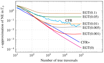
Figure 2: Regret as a function of the number of iterations for EGT with various ${\xi}$ perturbations (denoted in parentheses) and CFR+. Both axes are on a log scale.

The second experiment shows a measure of refinement convergence (Figure 3). The x-axis shows the number of tree traversals performed. The y-axis shows the maximum regret at any individual information set. Information set regret is calculated assuming that the information set is reached with probability one and applying Bayes’ rule to get a distribution over nodes at the information set; the regret is the increase in expected utility from best-responding throughout all information sets in the subtrees rooted at the information set. Both CFR+ and unperturbed EGT perform badly with respect to this measure of refinement. Both have maximum regret two orders of magnitude worse than the perturbed approach. The maximum regret one can possibly cause in an information set in Leduc 5 is 22, so CFR+ and unperturbed EGT also do poorly in that sense. In contrast to this, we find that our ${\xi}$-perturbed solution concepts converge to a strategy with low regret at every information set. The choice of ${\xi}$ is important: for ${\xi}=0.001$, the smallest perturbation, we see that it takes a long time to converge at low-probability information sets, whereas we converge reasonably quickly for ${\xi}=0.01$ or ${\xi}=0.005$; for ${\xi}=0.1$ and ${\xi}=0.05$ the perturbations are too large, and we end up converging with relatively high regret (due to being forced to play every action with probability ${\xi}$). Thus, within this set of experiments, ${\xi}\in\left[0.005,0.01\right]$ seems to be the ideal amount of perturbation.

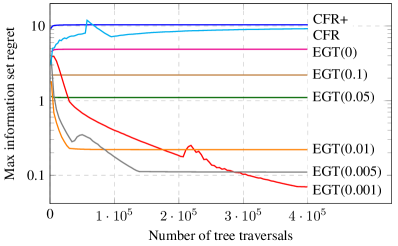
Figure 3: Maximum regret at any individual information set, as a function of the number of iterations.

5 Conclusion and future research

We studied the extension of FOMs to the computation of Nash-equilibrium refinements. We developed a smoothing scheme based on perturbations of smoothing schemes for standard EFG solving, and proved that the convergence rate is comparable to that of solving the original game for Nash equilibrium. We performed numerical simulations where we showed that our approach has an overall convergence rate that is comparable to that of state-of-the-art Nash equilibrium methods. At the same time, we showed that our approach leads to solutions that have substantially better performance in subsets of the game tree that are reached with low probability. This has benefits both in approximate Nash equilibrium finding (such approximation is necessary in practice in large games) where some probabilities are low while possibly heading toward zero in the limit, and exact Nash equilibrium computation where the low probabilities are actually zero.

Our work suggests several research directions. It would be interesting to find a way to systematically decrease the ${\xi}$-perturbations over time, so that we eventually converge to an exact Nash equilibrium in the full game. This requires at least two extensions. First, FOMs usually assume static domains, whereas this would involve a slowly expanding domain. Second, the ${\xi}$ would need to be decreased at a rate that is simultaneously fast enough that it converges at a reasonable rate, and slow enough that we actually converge to a refinement.

We showed how to compute approximate EFPE refinements using methods that scale to large games. It would be interesting to find a way to instantiate scalable methods such as FOMs or CFR+ for other equilibrium refinement concepts as well. The perturbed polytope due to Miltersen and Sørensen could be used to construct a notion of approximate QPE that would lead to an optimization setup similar to ours. However, this will require constructing a DGF for the perturbed-QPE polytope, which has ${\xi}$-perturbations on the realization plans. Our approach relied on ${\xi}$-perturbations to the behavioral strategies, and so it is likely that a different DGF class is needed to handle approximate QPE.

[ACPC] http://www.computerpokercompetition.org

References

- Bowling et al. [2015] Michael Bowling, Neil Burch, Michael Johanson, and Oskari Tammelin. Heads-up limit hold’em poker is solved. Science, 347(6218), January 2015.
- Brown and Sandholm [2015] Noam Brown and Tuomas Sandholm. Regret-based pruning in extensive-form games. In Proceedings of the Annual Conference on Neural Information Processing Systems (NIPS), 2015.
- Brown and Sandholm [2017a] N. Brown and T. Sandholm. Safe and Nested Subgame Solving for Imperfect-Information Games. ArXiv preprint arXiv:1705.02955, May 2017.
- Brown and Sandholm [2017b] Noam Brown and Tuomas Sandholm. Reduced space and faster convergence in imperfect-information games via pruning. In International Conference on Machine Learning (ICML), 2017.
- Brown et al. [2015] Noam Brown, Sam Ganzfried, and Tuomas Sandholm. Hierarchical abstraction, distributed equilibrium computation, and post-processing, with application to a champion no-limit Texas Hold’em agent. In International Conference on Autonomous Agents and Multi-Agent Systems (AAMAS), 2015.
- Chambolle and Pock [2011] Antonin Chambolle and Thomas Pock. A first-order primal-dual algorithm for convex problems with applications to imaging. Journal of Mathematical Imaging and Vision, 2011.
- Farina and Gatti [2017] Gabriele Farina and Nicola Gatti. Extensive-form perfect equilibrium computation in two-player games. In AAAI Conference on Artificial Intelligence (AAAI), 2017.
- Farina et al. [2017] Gabriele Farina, Christian Kroer, and Tuomas Sandholm. Regret minimization in behaviorally-constrained zero-sum games. In International Conference on Machine Learning (ICML), 2017.
- Gilpin and Sandholm [2007] Andrew Gilpin and Tuomas Sandholm. Lossless abstraction of imperfect information games. Journal of the ACM, 54(5), 2007.
- Hillas and Kohlberg [2002] John Hillas and Elon Kohlberg. Foundations of strategic equilibrium. Handbook of Game Theory with Economic Applications, 2002.
- Hoda et al. [2010] Samid Hoda, Andrew Gilpin, Javier Peña, and Tuomas Sandholm. Smoothing techniques for computing Nash equilibria of sequential games. Mathematics of Operations Research, 35(2), 2010.
- Koller et al. [1996] Daphne Koller, Nimrod Megiddo, and Bernhard von Stengel. Efficient computation of equilibria for extensive two-person games. Games and Economic Behavior, 14(2), 1996.
- Kroer et al. [2015] Christian Kroer, Kevin Waugh, Fatma Kılınç-Karzan, and Tuomas Sandholm. Faster first-order methods for extensive-form game solving. In Proceedings of the ACM Conference on Economics and Computation (EC), 2015.
- Kroer et al. [2017] Christian Kroer, Kevin Waugh, Fatma Kilinc-Karzan, and Tuomas Sandholm. Theoretical and practical advances on smoothing for extensive-form games. In Proceedings of the ACM Conference on Economics and Computation (EC), 2017.
- Lanctot et al. [2009] Marc Lanctot, Kevin Waugh, Martin Zinkevich, and Michael Bowling. Monte Carlo sampling for regret minimization in extensive games. In Proceedings of the Annual Conference on Neural Information Processing Systems (NIPS), 2009.
- Miltersen and Sørensen [2008] Peter Bro Miltersen and Troels Bjerre Sørensen. Fast algorithms for finding proper strategies in game trees. In Annual ACM-SIAM Symposium on Discrete Algorithms (SODA), 2008.
- Miltersen and Sørensen [2010] Peter Bro Miltersen and Troels Bjerre Sørensen. Computing a quasi-perfect equilibrium of a two-player game. Economic Theory, 42(1), 2010.
- Moravčík et al. [2017] Matej Moravčík, Martin Schmid, Neil Burch, Viliam Lisý, Dustin Morrill, Nolan Bard, Trevor Davis, Kevin Waugh, Michael Johanson, and Michael Bowling. Deepstack: Expert-level artificial intelligence in heads-up no-limit poker. Science, 356(6337), 2017.
- Nemirovski [2004] Arkadi Nemirovski. Prox-method with rate of convergence o(1/t) for variational inequalities with lipschitz continuous monotone operators and smooth convex-concave saddle point problems. SIAM Journal on Optimization, 15(1), 2004.
- Nesterov [2005a] Yurii Nesterov. Excessive gap technique in nonsmooth convex minimization. SIAM Journal of Optimization, 16(1), 2005.
- Nesterov [2005b] Yurii Nesterov. Smooth minimization of non-smooth functions. Mathematical Programming, 103, 2005.
- Romanovskii [1962] I. Romanovskii. Reduction of a game with complete memory to a matrix game. Soviet Mathematics, 3, 1962.
- Sandholm [2010] Tuomas Sandholm. The state of solving large incomplete-information games, and application to poker. AI Magazine, 2010. Special issue on Algorithmic Game Theory.
- Selten [1975] Reinhard Selten. Reexamination of the perfectness concept for equilibrium points in extensive games. International journal of game theory, 1975.
- Shoham and Leyton-Brown [2008] Yoav Shoham and Kevin Leyton-Brown. Multiagent systems: Algorithmic, game-theoretic, and logical foundations. Cambridge University Press, 2008.
- Southey et al. [2005] Finnegan Southey, Michael Bowling, Bryce Larson, Carmelo Piccione, Neil Burch, Darse Billings, and Chris Rayner. Bayes’ bluff: Opponent modelling in poker. In Proceedings of the 21st Annual Conference on Uncertainty in Artificial Intelligence (UAI), July 2005.
- Tammelin et al. [2015] Oskari Tammelin, Neil Burch, Michael Johanson, and Michael Bowling. Solving heads-up limit Texas hold’em. In Proceedings of the 24th International Joint Conference on Artificial Intelligence (IJCAI), 2015.
- van Damme [1984] Eric van Damme. A relation between perfect equilibria in extensive form games and proper equilibria in normal form games. International Journal of Game Theory, 1984.
- von Stengel et al. [2002] Bernhard von Stengel, Antoon Van Den Elzen, and Dolf Talman. Computing normal form perfect equilibria for extensive two-person games. Econometrica, 70(2), 2002.
- von Stengel [1996] Bernhard von Stengel. Efficient computation of behavior strategies. Games and Economic Behavior, 14(2), 1996.
- Zinkevich et al. [2007] Martin Zinkevich, Michael Bowling, Michael Johanson, and Carmelo Piccione. Regret minimization in games with incomplete information. In Proceedings of the Annual Conference on Neural Information Processing Systems (NIPS), 2007.