Convergent Tree Backup and Retrace with Function Approximation

Abstract

Off-policy learning is key to scaling up reinforcement learning as it allows to learn about a target policy from the experience generated by a different behavior policy. Unfortunately, it has been challenging to combine off-policy learning with function approximation and multi-step bootstrapping in a way that leads to both stable and efficient algorithms. In this work, we show that the Tree Backup and Retrace algorithms are unstable with linear function approximation, both in theory and in practice with specific examples. Based on our analysis, we then derive stable and efficient gradient-based algorithms using a quadratic convex-concave saddle-point formulation. By exploiting the problem structure proper to these algorithms, we are able to provide convergence guarantees and finite-sample bounds. The applicability of our new analysis also goes beyond Tree Backup and Retrace and allows us to provide new convergence rates for the GTD and GTD2 algorithms without having recourse to projections or Polyak averaging.

1 Introduction

Rather than being confined to their own stream of experience, off-policy learning algorithms are capable of leveraging data from a different behavior than the one being followed, which can provide many benefits: efficient parallel exploration as in Mnih et al. (2016) and Wang et al. (2016), reuse of past experience with experience replay (Lin, 1992) and, in many practical contexts, learning form data produced by policies that are currently deployed, but which we want to improve (as in many scenarios of working with an industrial or health care partner). Moreover, a single stream of experience can be used to learn about a variety of different targets which may take the form of value functions corresponding to different policies and time scales (Sutton et al., 1999) or to predicting different reward functions as in Sutton & Tanner (2004) and Sutton et al. (2011). Therefore, the design and analysis of off-policy algorithms using all the features of reinforcement learning, e.g. bootstrapping, multi-step updates (eligibility traces), and function approximation has been explored extensively over three decades. While off-policy learning and function approximation have been understood in isolation, their combination with multi-steps bootstrapping produces a so-called deadly triad (Sutton, 2015; Sutton & Barto, 2018), i.e., many algorithms in this category are unstable.

A convergent approach to this triad is provided by importance sampling, which bends the behavior policy distribution onto the target one (Precup, 2000; Precup et al., 2001). However, as the length of the trajectories increases, the variance of importance sampling corrections tends to become very large. The Tree Backup algorithm (Precup, 2000) is an alternative approach which remarkably does not rely on importance sampling ratios directly. More recently, Munos et al. (2016) introduced the Retrace algorithm which also builds on Tree Backup to perform off-policy learning without importance sampling.

Until now, Tree Backup and Retrace($\lambda$) had only been shown to converge in the tabular case, and their behavior with linear function approximation was not known. In this paper, we show that this combination with linear function approximation is in fact divergent. We obtain this result by analyzing the mean behavior of Tree Backup and Retrace using the ordinary differential equation (ODE) (Borkar & Meyn, 2000) associated with them. We also demonstrate this instability with a concrete counterexample.

Insights gained from this analysis allow us to derive a new gradient-based algorithm with provable convergence guarantees. Instead of adapting the derivation of Gradient Temporal Difference (GTD) learning from  (Sutton et al., 2009c), we use a primal-dual saddle point formulation (Liu et al., 2015; Macua et al., 2015) which facilitates the derivation of sample complexity bounds. The underlying saddle-point problem combines the primal variables, function approximation parameters, and dual variables through a bilinear term.

In general, stochastic primal-dual gradient algorithms like the ones derived in this paper can be shown to achieve $O(1/k)$ convergence rate (where $k$ is the number of iterations). For example, this has been established for the class of forward-backward algorithms with added noise  (Rosasco et al., 2016). Furthermore, this work assumes that the objective function is composed of a convex-concave term and a strongly convex-concave regularization term that admits a tractable proximal mapping. In this paper, we are able to achieve the same $O(1/k)$ convergence rate without having to assume strong convexity with respect to the primal variables and in the absence of proximal mappings. As corollary, our convergence rate result extends to the well-known gradient-based temporal difference algorithms GTD (Sutton et al., 2009c) and GTD2 (Sutton et al., 2009b) and hence improves the previously published results.

The algorithms resulting from our analysis are simple to implement, and perform well in practice compared to other existing multi-steps off-policy learning algorithms such as GQ($\lambda$) (Maei & Sutton, 2010) and AB-Trace($\lambda$) (Mahmood et al., 2017).

2 Background and notation

In reinforcement learning, an agent interacts with its environment which we model as discounted Markov Decision Process $(\mathcal{S},\mathcal{A},\gamma,P,r)$ with state space $\mathcal{S}$, action space $\mathcal{A}$, discount factor $\gamma\in[0,1)$, transition probabilities $P:\mathcal{S}\times\mathcal{A}\rightarrow(\mathcal{S}\rightarrow[0,1])$ mapping state-action pairs to distributions over next states, and reward function $r:(\mathcal{S}\times\mathcal{A})\rightarrow\mathbb{R}$. For simplicity, we assume the state and action space are finite, but our analysis can be extended to the countable or continuous case. We denote by $\pi(a\,|\,s)$ the probability of choosing action $a$ in state $s$ under the policy $\pi:\mathcal{S}\rightarrow(\mathcal{A}\rightarrow[0,1])$. The action-value function for policy $\pi$, denoted $Q^{\pi}:\mathcal{S}\times\mathcal{A}\rightarrow\mathbb{R}$, represents the expected sum of discounted rewards along the trajectories induced by the policy in the MDP: $Q^{\pi}(s,a)=\mathbb{E}\left[\sum_{t=0}^{\infty}\gamma^{t}r_{t}\,|\,(s_{0},a_{0})=(s,a),\pi\right]$. $Q^{\pi}$ can be obtained as the fixed point of the Bellman operator over the action-value function $\mathcal{T}^{\pi}Q=r+\gamma P^{\pi}Q$ where $r$ is the expected immediate reward and $P^{\pi}$ is defined as:

$$(P^{\pi}Q)(s,a)\triangleq\sum_{s^{\prime}\in\mathcal{S}}\sum_{a^{\prime}\in\mathcal{A}}P(s^{\prime}\,|\,s,a)\pi(a^{\prime}\,|\,s^{\prime})Q(s^{\prime},a^{\prime})\enspace.$$

In this paper, we are concerned with the policy evaluation problem (Sutton & Barto, 1998) under model-free off-policy learning. That is, we will evaluate a target policy $\pi$ using trajectories (i.e. sequences of states, actions and rewards) obtained from a different behavior policy $\mu$. In order to obtain generalization between different state-action pairs, $Q^{\pi}$ should be represented in a functional form. In this paper, we focus on linear function approximation of the form:

$$Q(s,a)\triangleq\theta^{\top}\phi(s,a)\enspace,$$

where $\theta\in\Theta\subset\mathbb{R}^{d}$ is a weight vector and $\phi:\mathcal{S}\times\mathcal{A}\rightarrow\mathbb{R}^{d}$ is a feature map from a state-action pairs to a given $d$-dimensional feature space.

Off-policy learning

(Munos et al., 2016) provided a unified perspective on several off-policy learning algorithms, namely: those using explicit importance sampling corrections  (Precup, 2000) as well as Tree Backup (TB($\lambda$)) (Precup, 2000) and $Q(\lambda)^{\pi}$ (Harutyunyan et al., 2016) which do not involve importance ratios. As a matter of fact, all these methods share a general form based on the $\lambda$-return (Sutton & Barto, 2018) but involve different coefficients $\kappa_{i}$ in :

$$G_{k}^{\lambda} \triangleq Q(s_{k},a_{k})+\sum_{t=k}^{\infty}(\lambda\gamma)^{t-k}\left(\prod_{i=k+1}^{t}\kappa_{i}\right)$$

$$\quad\times(r_{t}+\gamma\mathbb{E}_{\pi}Q(s_{t+1},\cdot)-Q(s_{t},a_{t}))$$

$$=Q(s_{k},a_{k})+\sum_{t=k}^{\infty}(\lambda\gamma)^{t-k}\left(\prod_{i=k+1}^{t}\kappa_{i}\right)\delta_{t}\enspace,$$

where $\mathbb{E}_{\pi}Q(s_{t+1},.)\triangleq\sum_{a\in\mathcal{A}}\pi(a\,|\,s_{t+1})Q(s_{t+1},a)$ and $\delta_{t}\triangleq r_{t}+\gamma\mathbb{E}_{\pi}Q(s_{t+1},.)-Q(s_{t},a_{t})$ is the temporal-difference (TD) error. The coefficients $\kappa_{i}$ determine how the TD errors would be scaled in order to correct for the discrepancy between target and behavior policies. From this unified representation, Munos et al. (2016) derived the Retrace($\lambda$) algorithm. Both TB($\lambda$) and Retrace($\lambda$) consider this form of return, but set $\kappa_{i}$ differently. The TB($\lambda$) updates correspond to the choice $\kappa_{i}=\pi(a_{i}\,|\,s_{i})$ while Retrace($\lambda$) sets $\kappa_{i}=\min\left(1,\frac{\pi(a_{i}\,|\,s_{i})}{\mu(a_{i}\,|\,s_{i})}\right)$, which is intended to allow learning from full returns when the target and behavior policies are very close. The importance sampling approach (Precup, 2000) converges in the tabular case by correcting the behavior data distribution to the distribution that would be induced by the target policy $\pi$. However, these correction terms lead to high variance in practice. Since $Q(\lambda)$ does not involve importance ratios, this variance problem is avoided but at the cost of restricted convergence guarantees satisfied only when the behavior and target policies are sufficiently close.

The analysis provided in this paper concerns TB($\lambda$) and Retrace($\lambda$), which are convergent in the tabular case, but have not been analyzed in the function approximation case. We start by noting that the Bellman operator $\mathcal{R}$ underlying these these algorithms can be written in the following form:

$$(\mathcal{R}Q)(s,a) \triangleq Q(s,a)+\mathbb{E}_{\mu}\Big{[}\sum_{t=0}^{\infty}(\lambda\gamma)^{t}\left(\prod_{i=1}^{t}\kappa_{i}\right)$$

$$\quad\times(r_{t}+\gamma\mathbb{E}_{\pi}Q(s_{t+1},\cdot)-Q(s_{t},a_{t}))\Big{]}$$

$$=Q(s,a)+(I-\lambda\gamma P^{\kappa\mu})^{-1}(\mathcal{T}^{\pi}Q-Q)(s,a)\enspace,$$

where $\mathbb{E}_{\mu}$ is the expectation over the behavior policy and MDP transition probabilities and $P^{\kappa\mu}$ is the operator defined by:

$$(P^{\kappa\mu}Q)(s,a)\triangleq\sum_{\begin{subarray}{c}s^{\prime}\in\mathcal{S}\\ a^{\prime}\in\mathcal{A}\end{subarray}}P(s^{\prime}\,|\,s,a)\mu(a^{\prime}\,|\,s^{\prime})\kappa(s^{\prime},a^{\prime})Q(s^{\prime},a^{\prime})\enspace.$$

In the tabular case, these operators were shown to be contraction mappings with respect to the max norm  (Precup, 2000; Munos et al., 2016). In this paper, we focus on what happens to these operators when combined with linear function approximation.

3 Off-policy instability with function approximation

When combined with function approximation, the temporal difference updates corresponding to the $\lambda$-return $G_{k}^{\lambda}$ are given by

$$\theta_{k+1} =\theta_{k}+\alpha_{k}\left(G_{k}^{\lambda}-Q(s_{k},a_{k})\right)\nabla_{\theta}Q(s_{k},a_{k})$$

$$=\theta_{k}+\alpha_{k}\left(\sum_{t=k}^{\infty}(\lambda\gamma)^{t-k}\left(\prod_{i=k+1}^{t}\kappa_{i}\right)\delta_{t}^{k}\right)\phi(s_{k},a_{k})$$ (1)

where $\delta_{t}^{k}=r_{t}+\gamma\theta_{k}^{\top}\mathbb{E}_{\pi}\phi(s_{t+1},\cdot)-\theta_{k}^{\top}\phi(s_{t},a_{t})$ and $\alpha_{k}$ are positive non-increasing step sizes. The updates (1) implies off-line updating as $G_{k}^{\lambda}$ is a quantity which depends on future rewards. This will be addressed later using eligibility traces: a mechanism to transform the off-line updates into efficient on-line ones. Since (1) describes stochastic updates, the following standard assumption is necessary:

Assumption 1.

The Markov chain induced by the behavior policy $\mu$ is ergodic and admits a unique stationary distribution, denoted by $\xi$, over state-action pairs. We write $\Xi$ for the diagonal matrix whose diagonal entries are $(\xi(s,a))_{s\in\mathcal{S},a\in\mathcal{A}}$.

Our first proposition establishes the expected behavior of the parameters in the limit.

Proposition 1.

If the behavior policy satisfies Assumption 1 and $(\theta_{k})_{k\leq 0}$ is the Markov process defined by (1) then:

$$\mathbb{E}[\theta_{k+1}\,|\,\theta_{0}]=\left(I+\alpha_{k}A\right)\mathbb{E}[\theta_{k}\,|\,\theta_{0}]+\alpha_{k}b\enspace,$$

where matrix $A$ and vector $b$ are defined as follows:

$$A \triangleq\Phi^{\top}\Xi(I-\lambda\gamma\mathit{P}^{\kappa\mu})^{-1}(\gamma\mathit{P}^{\pi}-I)\Phi\enspace,$$

$$b \triangleq\Phi^{\top}\Xi(I-\lambda\gamma P^{\kappa\mu})^{-1}r\enspace.$$

Sketch of Proof (The full proof is in the appendix).

$$\theta_{k+1} =\theta_{k}+\alpha_{k}\Big{(}\sum_{t=k}^{\infty}(\lambda\gamma)^{t-k}\left(\prod_{i=k+1}^{t}\kappa_{i}\right)\phi(s_{k},a_{k})$$

$$\quad\times\left([\gamma\mathbb{E}_{\pi}\phi(x_{t+1},\cdot)-\phi(x_{t},a_{t})]^{\top}\theta_{k}+r_{t}\right)\Big{)}$$

$$=\theta_{k}+\alpha_{k}\left(A_{k}\theta_{k}+b_{k}\right)\enspace.$$

So, $\mathbb{E}[\theta_{k+1}\,|\,\theta_{k}]=(I+\alpha_{k}A)\theta_{k}+\alpha_{k}b$ where $A=\mathbb{E}[A_{k}]$ and $b=\mathbb{E}[b_{k}]$ ∎

The ODE (Ordinary Differential Equations) approach (Borkar & Meyn, 2000) is the main tool to establish convergence in the function approximation case (Bertsekas & Tsitsiklis, 1995; Tsitsiklis et al., 1997). In particular, we use Proposition 4.8 in  Bertsekas & Tsitsiklis (1995), which states that under some conditions, $\theta_{k}$ converges to the unique solution $\theta^{*}$ of the system $A\theta^{*}+b=0$. This crucially relies on the matrix $A$ being negative definite i.e $y^{\top}Ay<0,\forall y\neq 0$. In the on-policy case, when $\mu=\pi$, we rely on the fact that the stationary distribution is invariant under the transition matrix $P^{\pi}$ i.e $d^{\top}P^{\pi}=d^{\top}$ (Tsitsiklis et al., 1997; Sutton et al., 2015). However, this is no longer true for off-policy learning with arbitrary target/behavior policies and the matrix $A$ may not be negative definite: the series $\theta_{k}$ may then diverge. We will now see that the same phenomenon may occur with TB($\lambda$) and Retrace($\lambda$).

Counterexample:

We extend the two-states MDP of Tsitsiklis et al. (1997), originally proposed to show the divergence of off-policy TD(0), to the case of function approximation over state-action pairs. This environment has only two states, as shown in Figure 1, and two actions: left or right.

Figure 1: Two-state counterexample. We assign the features $\{(1,0)^{\top},(2,0)^{\top},(0,1)^{\top},(0,2)^{\top}\}$ to the state-action pairs $\{(1,\text{right}),(2,\text{right}),(1,\text{left}),(2,\text{left})\}$. The target policy is given by $\pi(\text{right}\,|\,\cdot)=1$ and the behavior policy is $\mu(\text{right}\,|\,\cdot)=0.5$

In this particular case, both TB($\lambda$) and Retrace($\lambda$) share the same matrix $P^{\kappa\mu}$ and $P^{\kappa\mu}=0.5P^{\pi}$:

$$P^{\pi}=\left(\begin{matrix}0&1&0&0\\ 0&1&0&0\\ 1&0&0&0\\ 1&0&0&0\end{matrix}\right),(P^{\pi})^{n}=\left(\begin{matrix}0&1&0&0\\ 0&1&0&0\\ 0&1&0&0\\ 0&1&0&0\end{matrix}\right)\forall n\geq 2$$

If we set $\beta:=0.5\gamma\lambda$, we then have:

$$(I-\lambda\gamma P^{\kappa\mu})^{-1} =\left(\begin{matrix}1&\frac{\beta}{1-\beta}&0&0\\ 0&\frac{1}{1-\beta}&0&0\\ \beta&\frac{\beta^{2}}{1-\beta}&1&0\\ \beta&\frac{\beta^{2}}{1-\beta}&0&1\end{matrix}\right),$$

$$A =\left(\begin{matrix}\frac{6\gamma-\beta-5}{1-\beta}&0\\ \frac{3(\gamma\beta-\beta^{2}-\beta-\gamma)}{1-\beta}&-5\\ \end{matrix}\right)\enspace.$$

Therefore, $\forall\,\gamma\in(\frac{5}{6},1)$ and $\forall\,\lambda\in[0,\min(1,\frac{12\gamma-10}{\gamma}))$, the first eigenvalue $e_{1}=\frac{6\gamma-\beta-5}{1-\beta}$ of $A$ is positive. The basis vectors $(1,0)^{\top}$ and $(0,1)^{\top}$ are eigenvectors of A associated with $e_{1}$ and -5, then if $\theta_{0}=(\eta_{1},\eta_{2})^{\top}$, we obtain $\mathbb{E}[\theta_{k}\,|\,\theta_{0}]=(\eta_{1}\prod_{i=0}^{k-1}(1+\alpha_{i}e_{1}),\eta_{2}\prod_{i=0}^{k-1}(1-5\alpha_{i}))^{\top}$ implying that $||\mathbb{E}[\theta_{k}\,|\,\theta_{0}]||\geq|\eta_{1}|\prod_{i=0}^{k-1}(1+\alpha_{i}e_{1})$. Hence, as $\sum_{k}\alpha_{k}\rightarrow\infty$, $||\mathbb{E}[\theta_{k}\,|\,\theta_{0}]||\rightarrow\infty$ if $\eta_{1}\neq 0$.

4 Convergent gradient off-policy algorithms

If $A$ were to be negative definite, Retrace($\lambda$) or TB($\lambda$) with function approximation would converge to $\theta^{*}=-A^{-1}b$. It is known (Bertsekas, 2011) that $\Phi\theta^{*}$ is the fixed point of the projected Bellman operator :

$$\Phi\theta^{*}=\Pi^{\mu}\mathcal{R}(\Phi\theta^{*})\enspace,$$

where $\Pi^{\mu}=\Phi(\Phi^{\top}\Xi\Phi)^{-1}\Phi^{\top}\Xi$ is the orthogonal projection onto the space $S=\{\Phi\theta|\theta\in\mathbb{R}^{d}\}$ with respect to the weighted Euclidean norm $||.||_{\Xi}$. Rather than computing the sequence of iterates given by the projected Bellman operator, another approach for finding $\theta^{*}$ is to directly minimize (Sutton et al., 2009a; Liu et al., 2015) the Mean Squared Projected Bellman Error (MSPBE):

$$\mathbf{MSPBE}(\theta)=\frac{1}{2}||\Pi^{\mu}\mathcal{R}(\Phi\theta)-\Phi\theta||^{2}_{\Xi}\enspace.$$

This is the route that we take in this paper to derive convergent forms of TB($\lambda$) and Retrace($\lambda$). To do so, we first define our objective function in terms of $A$ and $b$ which we introduced in Proposition 1.

Proposition 2.

Let $M\triangleq\Phi^{\top}\Xi\Phi=\mathbb{E}[\Phi\Phi^{\top}]$ be the covariance matrix of features. We have:

$$\mathbf{MSPBE}(\theta)=\frac{1}{2}||A\theta+b||^{2}_{M^{-1}}$$

(The proof is provided in the appendix.)

In order to derive parameter updates, we could compute gradients of the above expression explicitly as in Sutton et al. (2009c), but we would then obtain a gradient that is a product of expectations. The implied double sampling makes it difficult to obtain an unbiased estimator of the gradient. Sutton et al. (2009c) addressed this problem with a two-timescale stochastic approximations. However, the algorithm obtained in this way is no longer a true stochastic gradient method with respect to the original objective.  Liu et al. (2015) suggested an alternative which converts the original minimization problem into a primal-dual saddle-point problem. This is the approach that we chose in this paper.

The convex conjugate of a real-valued function $f$ is defined as:

$$f^{*}(y)=\sup_{x\in\mathit{X}}(\langle y,x\rangle-f(x))\enspace,$$ (2)

and $f$ is convex, we have $f^{**}=f$. Also, if $f(x)=\frac{1}{2}||x||_{M^{-1}}$, then $f^{*}(x)=\frac{1}{2}||x||_{M}$. Note that by going to the convex conjugate, we do not need to invert matrix $M$. We now go back to the original minimization problem:

$$\min_{\theta}\mathbf{MSPBE}(\theta) \Leftrightarrow\min_{\theta}\frac{1}{2}||A\theta+b||_{M^{-1}}^{2}$$

$$\Leftrightarrow\min_{\theta}\max_{\omega}\left(\langle A\theta+b,\omega\rangle-\frac{1}{2}||\omega||_{M}^{2}\right)$$

The gradient updates resulting from the saddle-point problem (ascent in $\omega$ and descent in $\theta$) are then:

$$\omega_{k+1} =\omega_{k}+\eta_{k}(A\theta_{k}+b-M\omega_{k})\enspace,$$ (3)

$$\theta_{k+1} =\theta_{k}-\alpha_{k}A^{\top}\omega_{k}\enspace.$$

where $\{\eta_{k}\}$ and $\{\alpha_{k}\}$ are non-negative step-size sequences. As the $A$, $b$ and $M$ are all expectations, we can derive stochastic updates by drawing samples, which would yield unbiased estimates of the gradient.

On-line updates:

We now derive on-line updates by exploiting equivalences in expectation between forward views and backward views outlined in Maei (2011).

Proposition 3.

Let $e_{k}$ be the eligibility traces vector, defined as $e_{-1}=0$ and :

$$e_{k}=\lambda\gamma\kappa(s_{k},a_{k})e_{k-1}+\phi(s_{k},a_{k})\quad\forall k\geq 0\enspace.$$

Furthermore, let $\hat{A}_{k}=e_{k}(\gamma\mathbb{E}_{\pi}[\phi(s_{k+1},.)]-\phi(s_{k},a_{k})])^{\top},\quad\hat{b}_{k}=r(s_{k},a_{k})e_{k},\quad\hat{M}_{k}=\phi(s_{k},a_{k})\phi(s_{k},a_{k})^{\top}$. Then, we have $\mathbb{E}[\hat{A}_{k}]=A$, $\mathbb{E}[\hat{b}_{k}]=b$ and $\mathbb{E}[\hat{M}_{k}]=M$.

(The proof is provided in the appendix.)

This proposition allows us to replace the expectations in Eq. (3) by corresponding unbiased estimates. The resulting detailed procedure is provided in Algorithm 1.

Algorithm 1 Gradient Off-policy with eligibility traces

0:   target policy $\pi$, behavior policy $\mu$

  Initialize $\theta_{0}$ and $\omega_{0}$

  for n = 0 … do

     set $e_{0}=0$

     for k = 0 …end of episode do

        Observe $s_{k},a_{k},r_{k},s_{k+1}$ according to $\mu$

        Update traces

        $e_{k}=\lambda\gamma\kappa(s_{k},a_{k})e_{k-1}+\phi(s_{k},a_{k})$

        Update parameters

        $\delta_{k}=r_{k}+\gamma\theta_{k}^{\top}\mathbb{E}_{\pi}\phi(s_{k+1},.)-\theta_{k}^{\top}\phi(s_{k},a_{k})$

        $\omega_{k+1}=\omega_{k}+\eta_{k}\left(\delta_{k}e_{k}-\omega_{k}^{\top}\phi(s_{k},a_{k})\phi(s_{k},a_{k})\right)$

        $\theta_{k+1}=\theta_{k}-\alpha_{k}\omega_{k}^{\top}e_{k}\left(\gamma\mathbb{E}_{\pi}\phi(s_{k+1},.)-\phi(s_{k},a_{k})\right)$

     end for

  end for

5 Convergence Rate Analysis

In order to characterize the convergence rate of the algorithm 1, we need to introduce some new notations and state new assumptions.

We denote by $\|A\|\triangleq\sup_{\|x\|=1}\|Ax\|$ the spectral norm of the matrix A and by $c(A)=\|A\|\|A^{-1}\|$ its condition number. If the eigenvalues of a matrix $A$ are real, we use $\lambda_{\max}(A)$ and $\lambda_{\min}(A)$ to denote respectively the largest and the smallest eigenvalue.

If we set $\eta_{k}=\beta\alpha_{k}$ for a positive constant $\beta$, it is possible to combine the two iterations present in our algorithm as a single iteration using a parameter vector $z_{k}\triangleq\left(\begin{matrix}\theta_{k}\\ \frac{1}{\sqrt{\beta}}\omega_{k}\end{matrix}\right)$ where :

$$z_{k+1}=z_{k}-\alpha_{k}(\hat{G}_{k}z_{k}-\hat{g}_{k})$$

where:

$$\hat{G}_{k}\triangleq\left(\begin{matrix}0&\sqrt{\beta}\hat{A}_{k}^{\top}\\ -\sqrt{\beta}\hat{A}_{k}&\beta\hat{M}_{k}\end{matrix}\right)\quad\hat{g}_{k}\triangleq\left(\begin{matrix}0\\ \sqrt{\beta}\hat{b}_{k}\end{matrix}\right)$$

Let $G\triangleq\mathbb{E}\left[\hat{G}_{k}\right]$ and $g=\mathbb{E}\left[\hat{g}_{k}\right]$. It follows from the proposition 3 that $G$ and $g$ are well defined and more specifically:

$$G=\left(\begin{matrix}0&\sqrt{\beta}A^{\top}\\ -\sqrt{\beta}A&\beta M\end{matrix}\right)\quad g=\left(\begin{matrix}0\\ \sqrt{\beta}b\end{matrix}\right)$$

Furthermore, let $\mathcal{F}_{k}=\sigma(z_{0},\hat{G}_{0},\hat{g}_{0}\ldots,z_{k},\hat{G}_{k},\hat{g}_{k},z_{k+1})$ be the sigma-algebra generated by the variables up to time $k$. With these definitions, we can now state our assumptions.

Assumption 2.

The matrices $A$ and $M$ are nonsingular. This implies that the saddle-point problem admits a unique solution $(\theta^{\star},\omega^{\star})=(-A^{-1}b,0)$ and we define $z^{\star}\triangleq(\theta^{\star},\frac{1}{\sqrt{\beta}}\omega^{\star})$.

Assumption 3.

The features and reward functions are uniformly bounded. This implies that the features and rewards have uniformly bounded second moments. It follows that there exists a constant $\sigma$ such that:

$$\mathbb{E}[\|\hat{G}_{k}z_{k}-\hat{g}_{k}\|^{2}|\mathcal{F}_{k-1}]\leq\sigma^{2}(1+\|z_{k}\|^{2})$$

Before stating our main result, the following key quantities needs to be defined:

$$\rho\triangleq\lambda_{\max}(A^{\top}M^{-1}A),\quad\delta\triangleq\lambda_{\min}(A^{\top}M^{-1}A),$$

$$L_{G}\triangleq\Big{\|}\mathbb{E}\left[\hat{G}_{k}^{\top}\hat{G}_{k}\,|\,\mathcal{F}_{k-1}\right]\Big{\|}$$

The following proposition characterize the convergence in expectation of $\|z_{k}-z^{\star}\|^{2}=\|\theta_{k}-\theta^{\star}\|^{2}+\frac{1}{\beta}\|w_{k}\|^{2}$

Proposition 4.

Suppose assumptions 2 and 3 holds and if we choose $\beta=\frac{8\rho}{\lambda_{\min}(M)}$ and $\alpha_{k}=\frac{9^{2}\times 2\delta}{8\delta^{2}(k+2)+9^{2}\zeta}$ where $\zeta=2\times 9^{2}c(M)^{2}\rho^{2}+32c(M)L_{G}$. Then the mean square error $\mathbb{E}\left[\|z_{k}-z^{\star}\|^{2}\right]$ is upper bounded by:

$$9^{2}\times 8c(M)\Big{\{}\frac{(8\delta+9\zeta)^{2}\mathbb{E}\left[\|z_{0}-z^{\star}\|^{2}\right]}{(8^{2}\delta^{2}k+9^{2}\zeta)^{2}}+\frac{8\sigma^{2}(1+\|z^{\star}\|^{2})}{(8^{2}\delta^{2}k+9^{2}\zeta)}\Big{\}}$$

Sketch of Proof (The full proof is in the appendix).

The beginning of our proof relies on  Du et al. (2017) which shows the linear convergence rate of deterministic primal-dual gradient method for policy evaluation. More precisely, we make use of the spectral properties of matrix $G$ shown in the appendix of this paper. The rest of the proof follows a different route exploiting the structure of our problem. ∎

The above proposition 4 shows that the mean square error $\mathbb{E}\left[\|z_{k}-z^{\star}\|^{2}\right]$ at iteration $k$ is upper bounded by tow terms. The first bias term tells that the initial error $\mathbb{E}\left[\|z_{0}-z^{\star}\|^{2}\right]$ is forgotten at a rate $O(1/k^{2})$ and the constant depends on the condition number of the covariance matrix $c(M)$. The second variance term shows that noise is rejected at a rate $O(1/k)$ and the constant depends on the variance of estimates $\sigma^{2}$ and $c(M)$. The overall convergence rate is $O(1/k)$.

Existing stochastic saddle-point problem results:

Chen et al. (2014) provides a comprehensive review of stochastic saddle-point problem. When the objective function is convex-concave, the overall convergence rate is $O(1/\sqrt{k})$. Although several accelerated techniques could improve the dependencies on the smoothness constants of the problem in their convergence rate, the dominant term that depends on the gradient variance still decays only as $O(1/\sqrt{k})$.

When the objective function is strongly convex-concave,  Rosasco et al. (2016) and Palaniappan & Bach (2016) showed that stochastic forward-backward algorithms can achieve $O(1/k)$ convergence rate. Algorithms in this class are feasible in practice only if their proximal mappings can be computed efficiently. In our case, our objective function is strongly concave because of the positive-definiteness of $M$ but is otherwise not strongly convex. Because our algorithms are vanilla stochastic gradient methods, they do not rely on proximal mappings.

Singularity:

If assumption 2 does not hold, the matrix $G$ is singular and either $Gz+g=0$ has infinitely many solutions or it has no solution. In the case of many solutions, we could still get asymptotic convergence. In Wang & Bertsekas (2013), it was shown that under some assumptions on the null space of matrix $G$ and using a simple stabilization scheme, the iterates converge to the Drazin (Drazin, 1958) inverse solution of $Gz+g=0$. However, it is not clear how extend our finite-sample analysis because the spectral analysis of the matrix $G$ (Benzi & Simoncini, 2006) in our proof assumes that the matrices $A$ and $M$ are nonsingular.

6 Related Work and Discussion

Paper step-sizes Projection Polyak averaging Convergence rate  Sutton et al. (2009c),  Sutton et al. (2009b) $\eta_{k}=\beta\alpha_{k},\beta>0,$
$\sum_{k}\alpha_{k}=\infty,\sum_{k}\alpha_{k}^{2}<\infty$ No No $\theta_{k}\rightarrow\theta^{\star}$ with probability one  Liu et al. (2015) constant step-size, $\alpha_{k}=\eta_{k}$ Yes Yes $\mathbf{MSPBE}(\bar{\theta}_{k})\in O(1/\sqrt{k})$ with high probability  Wang et al. (2017) $\alpha_{k}=\eta_{k},\sum_{k}\alpha_{k}=\infty,$
$\frac{\sum_{k}\alpha_{k}^{2}}{\sum_{k}\alpha_{k}}<\infty$ Yes Yes $\mathbf{MSPBE}(\bar{\theta}_{k})\in O(\frac{\sum_{k}\alpha_{k}^{2}}{\sum_{k}\alpha_{k}})$ with high probability  Lakshminarayanan & Szepesvári (2017) constant step-size, $\alpha_{k}=\eta_{k}$ No Yes $\mathbb{E}[\|\bar{\theta}_{k}-\theta^{\star}\|^{2}]\in O(1/k)$  Dalal et al. (2017) $\alpha_{k}=\frac{1}{k^{1-c}},\eta_{k}=\frac{1}{k^{(2/3)(1-c)}}$
where $c\in(0,1)$ Yes No $\|\theta_{k}-\theta^{\star}\|\in O(k^{-\frac{1}{3}+\frac{c}{3}})$ with high probability Our work $\eta_{k}=\beta\alpha_{k},\beta>0,\alpha_{k}\in O(1/k)$ No No $\mathbb{E}[\|\theta_{k}-\theta^{\star}\|^{2}]\in O(1/k)$

Table 1: Convergence results for gradient-based TD algorithms shown in previous work (Sutton et al., 2009b, c; Liu et al., 2015; Wang et al., 2017; Lakshminarayanan & Szepesvári, 2017; Dalal et al., 2017). $\bar{\theta}_{k}$ stand for the Polyak-average of iterates: $\bar{\theta}_{k}\triangleq\frac{\sum_{k}\alpha_{k}\theta_{k}}{\sum_{k}\alpha_{k}}$. Our algorithms achieve $O(1/k)$ without the need for projections or Polyak averaging.

Convergent Retrace:

Mahmood et al. (2017) have recently introduced the ABQ($\zeta$) algorithm which uses an action-dependent bootstrapping parameter that leads to off-policy multi-step learning without importance sampling ratios. They also derived a gradient-based algorithm called AB-Trace($\lambda$) which is related to Retrace($\lambda$). However, the resulting updates are different from ours, as they use the two-timescale approach of Sutton et al. (2009a) as basis for their derivation. In contrast, our approach uses the saddle-point formulation, avoiding the need for double sampling. Another benefit of this formulation is that it allows us to provide a bound of the convergence rate (proposition 4) whereas  Mahmood et al. (2017) is restricted to a more general two-timescale asymptotic result from Borkar & Meyn (2000). The saddle-point formulation also provides a rich literature on acceleration methods which could be incorporated in our algorithms. Particularly in the batch setting,  Du et al. (2017) recently introduced Stochastic Variance Reduction methods for state-value estimation combining GTD with SVRG Johnson & Zhang (2013) or SAGA Defazio et al. (2014). This work could be extended easily to ours algorithms in the batch setting.

Existing Convergence Rates:

Our convergence rate result 4 can apply to GTD/GTD2 algorithms. Recall that GTD/GTD2 are off-policy algorithms designed to estimate the state-value function using temporal difference TD(0) return while our algorithms compute the action-value function using Retrace and Tree Backup returns. In both GTD and GTD2, the quantities $\hat{A}_{k}$ and $\hat{b}_{k}$ involved in their updates are the same and equal to $\hat{A}_{k}=\phi(s_{k})(\gamma\phi(s_{k+1})-\phi(s_{k}))^{\top}$, $\hat{b}_{k}=r(s_{k},a_{k})\phi(s_{k})$ while the matrix $\hat{M}_{k}$ is equal to $\phi(s_{k})\phi(s_{k})^{\top}$ for GTD2 and to identity matrix for GTD.
The table 1 show in chronological order the convergence rates established in the literature of Reinforcement learning. GTD was first introduced in  Sutton et al. (2009c) and its variant GTD2 was introduced later in  Sutton et al. (2009b). Both papers established the asymptotic convergence with Robbins-Monro step-sizes. Later, Liu et al. (2015) provided the first sample complexity by reformulating GTD/GTD2 as an instance of mirror stochastic approximation  (Nemirovski et al., 2009). Liu et al. (2015) showed that with high probability, $\mathbf{MSPBE}(\bar{\theta}_{k})\in O(1/\sqrt{k})$ where $\bar{\theta}_{k}\triangleq\frac{\sum_{k}\alpha_{k}\theta_{k}}{\sum_{k}\alpha_{k}}$. However, they studied an alternated version of GTD/GTD2 as they added a projection step into bounded convex set and Polyak-averaging of iterates. Wang et al. (2017) studied also the same version as  Liu et al. (2015) but for the case of Markov noise case instead of the i.i.d assumptions. They prove that with high probability $\mathbf{MSPBE}(\bar{\theta}_{k})\in O(\frac{\sum_{k}\alpha_{k}^{2}}{\sum_{k}\alpha_{k}})$ when the step-size sequence satisfies $\sum_{k}\alpha_{k}=\infty,\frac{\sum_{k}\alpha_{k}^{2}}{\sum_{k}\alpha_{k}}<\infty$. The optimal rate achieved in this setup is then $O(1/\sqrt{k})$. Recently, Lakshminarayanan & Szepesvári (2017) improved on the existing results by showing for the first time that $\mathbb{E}[\|\bar{\theta}_{k}-\theta^{\star}\|^{2}]\in O(1/k)$ without projection step. However, the result still consider the Polyak-average of iterates. Moreover, the constants in their bound depend on the data distribution that are difficult to relate to the problem-specific constants, such as those present in our bound 4. Finally, Dalal et al. (2017) studied sparsily projected version of GTD/GTD2 and they showed that for step-sizes $\alpha_{k}=\frac{1}{k^{1-c}},\eta_{k}=\frac{1}{k^{(2/3)(1-c)}}$ where $c\in(0,1)$, $\|\theta_{k}-\theta^{\star}\|\in O(k^{-\frac{1}{3}+\frac{c}{3}})$ with high probability. The projection is called sparse as they project only on iterations which are powers of 2.
Our work is the first to provide a finite-sample complexity analysis of GTD/GTD2 in its original setting, i.e without assumption a projection step or Polyak-averaging and with diminishing step-sizes.

7 Experimental Results

Evidence of instability in practice:

To validate our theoretical results about instability, we implemented TB($\lambda$), Retrace($\lambda$) and compared them against their gradient-based counterparts GTB($\lambda$) and GRetrace($\lambda$) derived in this paper. The first one is the $2$-states counterexample that we detailed in the third section and the second is the $7$-states versions of Baird’s counterexample (Baird et al., 1995). Figures 2 and 3 show the MSBPE (averaged over $20$ runs) as a function of the number of iterations. We can see that our gradient algorithms converge in these two counterexamples whereas TB($\lambda$) and Retrace($\lambda$) diverge.

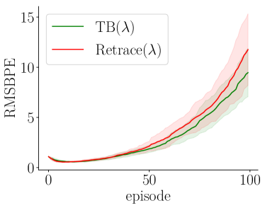
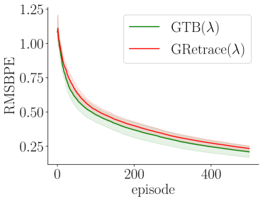
Figure 2: Baird’s counterexample. The combination of linear function approximation with TB and Retrace leads to divergence (left panel) while the proposed gradient extensions GTB and GRetrace converge (right panel).

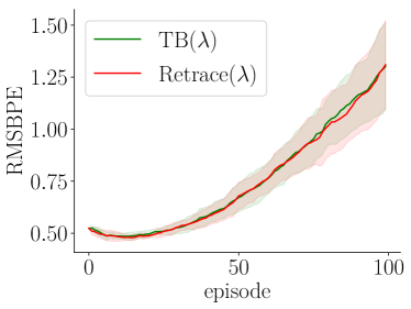
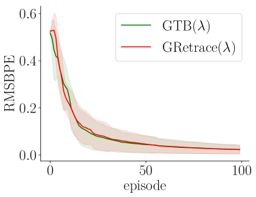
Figure 3: In the $2$-states counterexample of section 3 showing that the gradient-based TB and Retrace converge while TB and Retrace diverge.

Comparison with existing methods:

We also compared GTB($\lambda$) and GRetrace($\lambda$) with two recent state-of-the-art convergent off-policy algorithms for action-value estimation and function approximation: GQ($\lambda$) (Maei, 2011) and AB-Trace($\lambda$) (Mahmood et al., 2017). As in  Mahmood et al. (2017), we also consider a policy evaluation task in the Mountain Car domain. In order to better understand the variance inherent to each method, we designed the target policy and behavior policy in such a way that the importance sampling ratios can be as large as $30$. We chose to describe state-action pairs by a $96$-dimensional vector of features derived by tile coding (Sutton & Barto, 1998). We ran each algorithm over all possible combinations of step-size values $(\alpha_{k},\eta_{k})\in[0.001,0.005,0.01,0.05,0.1]^{2}$ for $2000$ episodes and reported their normalized mean squared errors (NMSE):

$$\mathbf{NMSE}(\theta)=\frac{\|\Phi\theta-Q^{\pi}\|^{2}_{\Xi}}{\|Q^{\pi}\|^{2}_{\Xi}}$$

where $Q^{\pi}$ is estimated by simulating the target policy and averaging the discounted cumulative rewards overs trajectories. As AB-Trace($\lambda$) and GRetrace($\lambda$) share both the same operator, we can evaluate them using the empirical $\mathbf{MSPBE}=\frac{1}{2}||\hat{A}\theta+\hat{b}||^{2}_{\hat{M}^{-1}}$ where $\hat{A}$, $\hat{b}$ and $\hat{M}$ are Monte-Carlo estimates obtained by averaging $\hat{A}_{k}$, $\hat{b}_{k}$ and $\hat{M}_{k}$ defined in proposition 3 over $10000$ episodes.
Figure 6 shows that the best empirical $\mathbf{MSPBE}$ achieved by AB-Trace($\lambda$) and GRetrace($\lambda$) are almost identical across value of $\lambda$. This result is consistent with the fact that they both minimize the $\mathbf{MSPBE}$ objective function. However, significant differences can be observed when computing the 5th percentiles of NMSE (over all possible combination of step-size values) for different values of $\lambda$ in Figure 5. When $\lambda$ increases, the NMSE of GQ($\lambda$) increases sharply due to increased influence of importance sampling ratios. This clearly demonstrate the variance issues of GQ($\lambda$) in contrast with the other methods based on the Tree Backup and Retrace returns (that are not using importance ratios). For intermediate values of $\lambda$, AB-Trace($\lambda$) performs better but its performance is matched by GRetrace($\lambda$) and TB($\lambda$) for small and very large values of $\lambda$. In fact, AB-Trace($\lambda$) updates the function parameters $\theta$ as follows:

$$\theta_{k+1}=\theta_{k}-\alpha_{k}\left(\delta_{k}e_{k}-\Delta_{k}\right)$$

where $\Delta_{k}\triangleq\gamma w_{k}^{\top}e_{k}(\mathbb{E}_{\pi}\phi(s_{k+1},.)-\lambda\sum_{a}\kappa(s_{k},a)\mu(a\,|\,s_{k})\phi(s_{k},a))$ is a gradient correction term. When the instability is not an issue, the correction term could be very small and the update of $\theta$ would be essentially $\theta_{k+1}\sim\theta_{k}-\alpha_{k}\delta_{k}e_{k}$ so that $\theta_{k+1}$ follows the semi-gradient of the mean squared error $\|\Phi\theta-G^{\lambda}_{k}\|^{2}_{\Xi}$.
To better understand the errors of each algorithm and their robustness to step-size values, we propose the box plots shown in Figure 4. Each box plot shows the distribution of NMSE obtained by each algorithm for different values of $\lambda$. NMSE distributions are computed over all possible combinations of step-size values. GTB($\lambda$) has the smallest variance as it scaled its return by the target probabilities which makes it conservative in its update even with large step-size values. GRetrace($\lambda$) tends to more more efficient than GTB($\lambda$) since it could benefit from full returns. The latter observation agrees with the tabular case of Tree Backup and Retrace (Munos et al., 2016). Finally, we observe that AB-Trace($\lambda$) has lower error, but at the cost of increased variance with respect to step-size values.

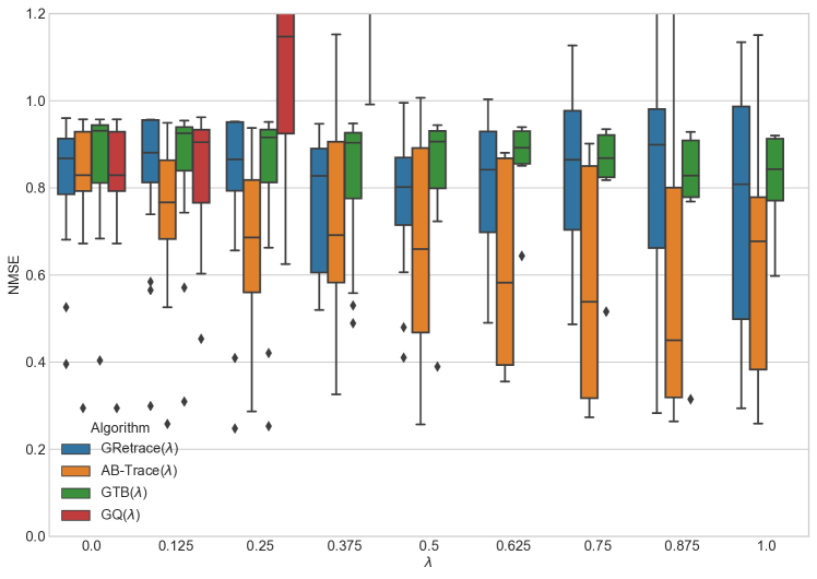
Figure 4: Comparison of empirical performance of GQ($\lambda$), AB-Trace($\lambda$), GRetrace($\lambda$) and GTB($\lambda$) on an off-policy evaluation task in Mountain Car domain. Each box plot shows the distribution of the NMSE achieved by each algorithm after 2000 episodes for different values of $\lambda$. NMSE distributions are computed over all the possible combinations of step-size values $(\alpha_{k},\eta_{k})\in[0.001,0.005,0.01,0.05,0.1]^{2}$.

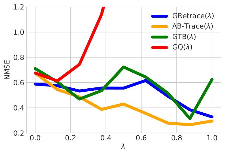
Figure 5: Each curves shows the 5th percentile of NMSE (over all possible combination of step-size values) achieved by each algorithm for different values of $\lambda$.

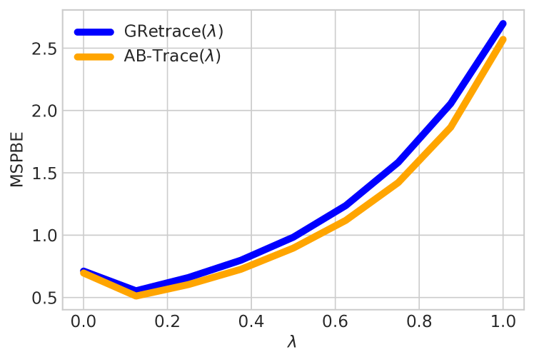
Figure 6: Comparison between the best empirical MSPBE obtained by each algorithm for different values of $\lambda$. Only GRetrace($\lambda$) and AB-Trace($\lambda$) are showed here because the other algorithms do not have the same operators and hence not the same $\mathbf{MSPBE}$. Note that $\mathbf{MSPBE}$s depend on $\lambda$. Thus, $\mathbf{MSPBE}$s are not directly comparable across different values of $\lambda$. Both GRetrace($\lambda$) and AB-Trace($\lambda$) have very similar performances. AB-Trace($\lambda$) performs slightly better.

8 Conclusion

Our analysis highlighted for the first time the difficulties of combining the Tree Backup and Retrace algorithms with function approximation. We addressed these issues by formulating gradient-based algorithm versions of these algorithms which minimize the mean-square projected Bellman error. Using a saddle-point formulation, we were also able to provide convergence guarantees and characterize the convergence rate of our algorithms GTB and GRetrace. We also developed a novel analysis method which allowed us to establish a $O(1/k)$ convergence rate without having to use Polyak averaging or projections (which might also make implementation more difficult). Furthermore, our proof technique is general enough that we were able to apply it to the existing GTD and GTD2 algorithms. Our experiments finally suggest that the proposed GTB($\lambda$) and GRetrace ($\lambda$) are robust to step-size selection and have less variance than both GQ($\lambda$) (Maei, 2011) and AB-Trace($\lambda$) (Mahmood et al., 2017).

Appendix A Proof of Proposition 1

We compute $\mathbb{E}[A_{k}]$ and $\mathbb{E}[b_{k}]$ where expectation are over trajectories drawn by executing the behavior policy: $s_{k},a_{k},r_{k},s_{k+1},\ldots s_{t},a_{t},r_{t},s_{t+1}\ldots$ where $s_{k},a_{k}\sim d,\quad r_{t}=r(s_{t},a_{t}),\quad s_{t+1}\sim p(\cdot\,|\,s_{t},a_{t})$. We note that under stationarity of $d$, $\mathbb{E}[A_{k}]=E[A_{0}]$ and $\mathbb{E}[b_{k}]=\mathbb{E}[b_{0}]$. Let $\theta,\theta^{\prime}\in\mathcal{R}^{d}$ and let $Q=\Phi\theta$ and $Q^{\prime}=\Phi\theta^{\prime}$ their respective Q-functions.

$$\theta^{\prime\top}\mathbb{E}[A_{k}]\theta =\mathbb{E}\left[\sum_{t=0}^{\infty}(\lambda\gamma)^{t}\left(\prod_{i=1}^{t}\kappa_{i}\right)Q^{\prime}(s_{0},a_{0})[\gamma\mathbb{E}_{\pi}Q(s_{t+1},.)-Q(s_{t},a_{t})]^{\top}\right]$$

$$=\sum_{t=0}^{\infty}(\lambda\gamma)^{t}\mathbb{E}_{\begin{subarray}{c}s_{0:t+1}\\ a_{0:t}\end{subarray}}\left[Q^{\prime}(s_{0},a_{0})\left(\prod_{i=1}^{t}\kappa_{i}\right)[\gamma\mathbb{E}_{\pi}Q(s_{t+1},.)-Q(s_{t},a_{t})]^{\top}\right]$$

$$=\sum_{t=0}^{\infty}(\lambda\gamma)^{t}\mathbb{E}_{\begin{subarray}{c}s_{0:t}\\ a_{0:t}\end{subarray}}\left[Q^{\prime}(s_{0},a_{0})\left(\prod_{i=1}^{t}\kappa_{i}\right)(\gamma\mathbb{E}_{s_{t+1}}[\mathbb{E}_{\pi}Q(s_{t+1},.)|s_{t},a_{t}]-Q(s_{t},a_{t}))\right]$$

$$=\sum_{t=0}^{\infty}(\lambda\gamma)^{t}\mathbb{E}_{\begin{subarray}{c}s_{0:t}\\ a_{0:t}\end{subarray}}\left[Q^{\prime}(s_{0},a_{0})\left(\prod_{i=1}^{t}\kappa_{i}\right)(\gamma\sum_{s^{\prime}\in\mathcal{S}}\sum_{a^{\prime}\in\mathcal{A}}p(s^{\prime}|s_{t},a_{t})\pi(a^{\prime}|s^{\prime})Q(s^{\prime},a^{\prime})-Q(s_{t},a_{t}))\right]$$

$$=\sum_{t=0}^{\infty}(\lambda\gamma)^{t}\mathbb{E}_{\begin{subarray}{c}s_{0:t}\\ a_{0:t}\end{subarray}}\left[Q^{\prime}(s_{0},a_{0})\left(\prod_{i=1}^{t}\kappa_{i}\right)(\gamma P^{\pi}Q(s_{t},a_{t})-Q(s_{t},a_{t}))\right]$$

$$=\sum_{t=0}^{\infty}(\lambda\gamma)^{t}\mathbb{E}_{\begin{subarray}{c}s_{0:t-1}\\ a_{0:t-1}\end{subarray}}\left[Q^{\prime}(s_{0},a_{0})\left(\prod_{i=1}^{t-1}\kappa_{i}\right)\sum_{s^{\prime}\in\mathcal{S}}\sum_{a^{\prime}\in\mathcal{A}}p(s^{\prime}|s_{t-1},a_{t-1})\kappa(a^{\prime},s^{\prime})\mu(a^{\prime}|s^{\prime})(\gamma P^{\pi}Q(s^{\prime},a^{\prime})-Q(s^{\prime},a^{\prime}))\right]$$

$$=\sum_{t=0}^{\infty}(\lambda\gamma)^{t}\mathbb{E}_{\begin{subarray}{c}s_{0:t-1}\\ a_{0:t-1}\end{subarray}}\left[Q^{\prime}(s_{0},a_{0})\left(\prod_{i=1}^{t-1}\kappa_{i}\right)P^{\kappa\mu}(\gamma P^{\pi}-I)Q(s_{t-1},a_{t-1})\right]$$

$$=\mathbb{E}_{s_{0},a_{0}}\left[Q^{\prime}(s_{0},a_{0})\sum_{t=0}^{\infty}(\lambda\gamma)^{t}(P^{\kappa\mu})^{t}(\gamma P^{\pi}-I)Q(x_{0},a_{0})\right]$$

$$=\mathbb{E}_{s_{0},a_{0}}\left[Q^{\prime}(s_{0},a_{0})(I-\lambda\gamma P^{\kappa\mu})^{-1}(\gamma P^{\pi}-I)Q(s_{0},a_{0})\right]$$

$$=\sum_{s\in\mathcal{S}}\sum_{a\in\mathcal{A}}\xi(s,a)Q^{\prime}(s,a)(I-\lambda\gamma P^{\kappa\mu})^{-1}(\gamma P^{\pi}-I)Q(s,a)$$

$$=Q^{\prime\top}\Xi(I-\lambda\gamma P^{\kappa\mu})^{-1}(\gamma P^{\pi}-I)Q$$

So, $\theta^{\prime\top}\mathbb{E}[A_{k}]\theta=\theta^{\prime\top}\Phi^{\top}\Xi(I-\lambda\gamma P^{\kappa\mu})^{-1}(\gamma P^{\pi}-I)\Phi\theta\quad\forall\theta,\theta^{\prime}\in\mathcal{R}^{d}$, which implies that:

$$\mathbb{E}[A_{k}]=\Phi^{\top}\Xi(I-\lambda\gamma P^{\kappa\mu})^{-1}(P^{\pi}-I)\Phi$$

$$\theta^{\top}\mathbb{E}[b_{k}] =\mathbb{E}[\sum_{t=0}^{\infty}(\lambda\gamma)^{t}\left(\prod_{i=1}^{t}\kappa_{i}\right)r_{t}Q(s_{0},a_{0})]=\sum_{t=0}^{\infty}(\lambda\gamma)^{t}\mathbb{E}_{\begin{subarray}{c}s_{0:t}\\ a_{0:t}\end{subarray}}\left[Q(s_{0},a_{0})\left(\prod_{i=1}^{t}\kappa_{i}\right)r(s_{t},a_{t})\right]$$

$$=\sum_{t=0}^{\infty}(\lambda\gamma)^{t}\mathbb{E}_{\begin{subarray}{c}s_{0:t-1}\\ a_{0:t-1}\end{subarray}}\left[Q(s_{0},a_{0})\left(\prod_{i=1}^{t-1}\kappa_{i}\right)\sum_{s^{\prime}\in\mathcal{S}}\sum_{a^{\prime}\in\mathcal{A}}p(s^{\prime}|s_{t-1},a_{t-1})\kappa(a^{\prime},s^{\prime})\mu(a^{\prime}|s^{\prime})r(s^{\prime},a^{\prime})\right]$$

$$=\sum_{t=0}^{\infty}(\lambda\gamma)^{t}\mathbb{E}_{\begin{subarray}{c}s_{0:t-1}\\ a_{0:t-1}\end{subarray}}\left[Q(s_{0},a_{0})\left(\prod_{i=1}^{t-1}\kappa_{i}\right)P^{\kappa\mu}r(s^{\prime},a^{\prime})\right]=\mathbb{E}_{s_{0},a_{0}}\left[Q(s_{0},a_{0})(I-\lambda\gamma P^{\kappa\mu})^{-1}r(s_{0},s_{0})\right]$$

$$=\sum_{s\in\mathcal{S}}\sum_{a\in\mathcal{A}}\xi(s,a)Q(s,a)(I-\lambda\gamma P^{\kappa\mu})^{-1}r(s,a)=Q^{\top}\Xi(I-\lambda\gamma P^{\kappa\mu})^{-1}r$$

So, $\theta^{\top}\mathbb{E}[b_{k}]=\theta^{\top}\Phi^{\top}\Xi(I-\lambda\gamma P^{\kappa\mu})^{-1}r\quad\forall\theta\in\mathcal{R}^{d}$, which implies that:

$$\mathbb{E}[b_{k}]=\Phi^{\top}\Xi(I-\lambda\gamma P^{\kappa\mu})^{-1}r$$

Appendix B Proof of Proposition 2

$$\mathbf{MSPBE}(\theta) =\frac{1}{2}||\Pi^{\mu}\mathcal{R}(\Phi\theta)-\Phi\theta||^{2}_{\Xi}=\frac{1}{2}||\Pi^{\mu}\left(\mathcal{R}(\Phi\theta)-\Phi\theta\right)||^{2}_{\Xi}$$

$$=\frac{1}{2}\left(\Pi^{\mu}\left(\mathcal{R}(\Phi\theta)-\Phi\theta\right)\right)^{\top}\Xi\left(\Pi^{\mu}\left(\mathcal{R}(\Phi\theta)-\Phi\theta\right)\right)$$

$$=\frac{1}{2}\left(\Phi^{\top}\Xi\left(\mathcal{R}(\Phi\theta)-\Phi\theta\right)\right)^{\top}(\Phi^{\top}\Xi\Phi)^{-1}\Phi^{\top}\Xi\left(\Phi(\Phi^{\top}\Xi\Phi)^{-1}\Phi^{\top}\Xi(\mathcal{R}(\Phi\theta)-\Phi\theta)\right)$$

$$=\frac{1}{2}||\Phi^{\top}\Xi\left(\mathcal{R}(\Phi\theta)-\Phi\theta\right)||^{2}_{M^{-1}}$$

$$=\frac{1}{2}||\Phi^{\top}\Xi\left((I-\lambda\gamma P^{\mu\pi})^{-1}(\mathcal{T}^{\pi}-\lambda\gamma P^{\mu\pi})\Phi\theta-\Phi\theta\right)||^{2}_{M^{-1}}$$

$$=\frac{1}{2}||\Phi^{\top}\Xi(I-\lambda\gamma P^{\mu\pi})^{-1}(\gamma\mathit{P}^{\pi}-I)\Phi\theta+\Phi^{\top}\Xi(I-\lambda\gamma P^{\mu\pi})^{-1}r||^{2}_{M^{-1}}$$

$$=\frac{1}{2}||A\theta+b||^{2}_{M^{-1}}$$

Appendix C Proof of Proposition 3

Let’s show that $\mathbb{E}[\hat{A}_{k}]=A$. Let’s $\Delta_{t}$ denotes $[\gamma\mathbb{E}_{\pi}\phi(s_{t+1},.)^{\top}-\phi(s_{t},a_{t})^{\top}]$

$$A =\mathbb{E}\left[\sum_{t=k}^{\infty}(\lambda\gamma)^{t-k}\left(\prod_{i=k+1}^{t}\kappa_{i}\right)\phi(s_{k},a_{k})\Delta_{t}\right]$$

$$=\mathbb{E}\left[\phi(s_{k},a_{k})\Delta_{k}+\sum_{t=k+1}^{\infty}(\lambda\gamma)^{t-k}\left(\prod_{i=k+1}^{t}\kappa_{i}\right)\phi(s_{k},a_{k})\Delta_{t}\right]$$

$$=\mathbb{E}\left[\phi(s_{k},a_{k})\Delta_{k}+\sum_{t=k}^{\infty}(\lambda\gamma)^{t-k+1}\left(\prod_{i=k+1}^{t+1}\kappa_{i}\right)\phi(s_{k},a_{k})\Delta_{t+1}\right]$$

$$=\mathbb{E}\left[\phi(s_{k},a_{k})\Delta_{k}+\lambda\gamma\kappa(s_{k+1},a_{k+1})\phi(s_{k},a_{k})\Delta_{k+1}+\sum_{t=k+1}^{\infty}(\lambda\gamma)^{t-k+1}\left(\prod_{i=k+1}^{t+1}\kappa_{i}\right)\phi(s_{k},a_{k})\Delta_{t+1}\right]$$

$$\stackrel{{\scriptstyle(\star)}}{{=}}\mathbb{E}\left[\phi(s_{k},a_{k})\Delta_{k}+\lambda\gamma\kappa(s_{k},a_{k})\phi(s_{k-1},a_{k-1})\Delta_{k}+\sum_{t=k+1}^{\infty}(\lambda\gamma)^{t-k+1}\left(\prod_{i=k+1}^{t+1}\kappa_{i}\right)\phi(s_{k},a_{k})\Delta_{t+1}\right]$$

$$=\mathbb{E}\left[\Delta_{k}(\phi(s_{k},a_{k})+\lambda\gamma\kappa(s_{k},a_{k})\phi(s_{k-1},a_{k-1})+(\lambda\gamma)^{2}\kappa(s_{k},a_{k})\kappa(s_{k-1},a_{k-1})\phi(s_{k-2},a_{k-2})+...)\right]$$

$$=\mathbb{E}\left[\Delta_{k}\left(\sum_{i=0}^{k}(\lambda\gamma)^{k-i}\left(\prod_{j=i+1}^{k}\kappa_{j}\right)\phi(x_{i},a_{i})\right)\right]$$

$$=\mathbb{E}[\Delta_{k}e_{k}]=\mathbb{E}[\hat{A}_{k}]$$

we have used in the line ($\star$) the fact that $\mathbb{E}[\kappa(s_{k+1},a_{k+1})\phi(s_{k}a_{k})\Delta_{k+1}]=\mathbb{E}[\kappa(s_{k},a_{k})\phi(s_{k-1}a_{k-1})\Delta_{k}]$ thanks to the stationarity of the distribution $d$.
we have also denote by $e_{k}$ the following vector:

$$e_{k} =\sum_{i=0}^{k}(\lambda\gamma)^{k-i}\left(\prod_{j=i+1}^{k}\kappa_{j}\right)\phi(s_{i},a_{i})$$

$$=\lambda\gamma\kappa_{k}\left(\sum_{i=0}^{k-1}(\lambda\gamma)^{k-1-i}\left(\prod_{j=i+1}^{k-1}\kappa_{j}\right)\phi(s_{i},a_{i})\right)+\phi(s_{k},a_{k})$$

$$=\lambda\gamma\kappa_{k}e_{k-1}+\phi(s_{k},a_{k})$$

Vector $e_{k}$ corresponds to the eligibility traces defined in the proposition. Similarly, we could show that $\mathbb{E}_{\mu}[\hat{b}_{k}]=b$.

Appendix D True on-line equivalence

In (van Hasselt et al., 2014), the authors derived a true on-line update for GTD($\lambda$) that empirically performed better than GTD($\lambda$) with eligibility traces. Based on this work, we derive true on-line updates for our algorithm. The gradient off-policy algorithm was derived by turning the expected forward view into an expected backward view which can be sampled. In order to derive a true on-line update, we sample instead the forward view and then we turn the sampled forward view to an exact backward view using Theorem 1 in (van Hasselt et al., 2014). If $k$ denotes the time horizon, we consider the sampled truncated interim forward return:

$$\forall t<k,\quad Y_{t}^{k}=\sum_{i=t}^{k-1}(\lambda\gamma)^{i-t}\left(\prod_{j=t+1}^{i}\kappa_{j}\right)\delta_{i}$$

where $\delta_{i}=r_{i}+\theta_{t}^{\top}\mathbb{E}_{\pi}\phi(s_{t+1},\cdot)-\theta_{t}^{\top}\phi(s_{t},a_{t})$, which gives us the sampled forward update of $\omega$:

$$\forall k<t,\quad\omega_{t+1}^{k}=\omega_{t}^{k}+\alpha_{t}(Y_{t}^{k}-\phi(x_{t},a_{t})^{\top}\omega_{t}^{k})\phi(x_{t},a_{t})$$ (4)

Proposition 5.

For any k, the parameter $\omega_{k}^{k}$ defined by the forward view (4) is equal to $\omega_{k}$ defined by the following backward view:

$$e^{\omega}_{-1} =0,\quad\forall k\geq 0$$

$$e^{\omega}_{k} =\lambda\gamma\kappa_{k}e^{\omega}_{k-1}+\alpha_{k}(1-\lambda\gamma\kappa_{k}\phi(s_{k},a_{k})^{\top}e^{\omega}_{k-1})\phi(s_{k},a_{k})$$

$$\omega_{k+1} =\omega_{k}+\delta_{k}e^{\omega}_{k}-\alpha_{t}\phi(s_{k},a_{k})^{\top}\omega_{k}\phi(s_{k},a_{k})$$

Proof.

The return’s temporal difference $Y_{t}^{k+1}-Y_{t}^{k}$ are related through:

$$\forall t<k,\quad Y_{t}^{k+1}-Y_{t}^{k} =\sum_{i=t}^{k}(\lambda\gamma)^{i-t}(\prod_{j=t+1}^{i}\kappa_{j})\delta_{i}-\sum_{i=t}^{k-1}(\lambda\gamma)^{i-t}(\prod_{j=t+1}^{i}\kappa_{j})\delta_{i}$$

$$=(\lambda\gamma)^{k-t}\left(\prod_{j=t+1}^{k}\kappa_{j}\right)\delta_{k}$$

$$=\lambda\gamma\kappa_{k+1}\left((\lambda\gamma)^{k-(t+1)}\left(\prod_{j=t+2}^{k}\kappa_{j}\right)\delta_{k}\right)$$

$$=\lambda\gamma\kappa_{k+1}\left(Y_{t+1}^{k+1}-Y_{t+1}^{k}\right)$$

We could then apply Theorem 1 of (van Hasselt et al., 2014) that give us the following backward view:

$$e_{0} =\alpha_{0}\phi(x_{0},a_{0})$$

$$e_{t} =\lambda\gamma\kappa_{t}e_{t-1}+\alpha_{t}(1-\lambda\gamma\kappa_{k}\phi(s_{t},a_{t})^{\top}e_{t-1})\phi(s_{t},a_{t})\quad\forall t>0$$

$$\omega_{t+1} =\omega_{t}+(Y_{t}^{t+1}-Y_{t}^{t})e_{t}+\alpha_{t}(Y_{t}^{t}-\phi(s_{t},a_{t})^{\top}\omega_{t})\phi(s_{t},a_{t})$$

$$\stackrel{{\scriptstyle(\star)}}{{=}}\omega_{t}+\delta_{t}e_{t}-\alpha_{t}\phi(s_{t},a_{t})^{\top}\omega_{t}\phi(s_{t},a_{t})$$

We used in the line ($\star$) that $Y_{t}^{t+1}=\delta_{t}$ and $Y_{t}^{t}=0$ ∎

The resulting detailed procedure is provided in Algorithm 2.

Note that when $\lambda$ is equal to zero, the Algorithm 1 and 2 both reduce to the same update:

$$\omega_{k+1} =\omega_{k}+\alpha_{k}(\delta_{k}-\phi(s_{k},a_{k})^{\top}\omega_{k})\phi(s_{k},a_{k})$$

$$\theta_{k+1} =\theta_{k}-\alpha_{k}\phi(s_{k},a_{k})^{\top}w_{k}(\gamma\mathbb{E}_{\pi}[\phi(s_{k+1},.)]-\phi(s_{k},a_{k})])$$

Algorithm 2 Gradient Off-policy with eligibility/Dutch traces

0:   target policy $\pi$, behavior policy $\mu$

  Initialize $\theta_{0}$ and $\omega_{0}$

  for n = 0 … do

     set $e^{\theta}_{-1}=e^{\omega}_{-1}=0$

     for k = 0 …end of episode do

        Observe $s_{k},a_{k},r_{k},s_{k+1}$ according to $\mu$

        Update traces

        $e_{k}=\lambda\gamma\kappa(s_{k},a_{k})e_{k-1}+\phi(s_{k},a_{k})$

        Update Dutch traces

        $e^{\omega}_{k}=\lambda\gamma\kappa_{k}e^{\omega}_{k-1}+\alpha_{k}\left(1-\lambda\gamma\kappa_{k}\phi(s_{k},a_{k})^{\top}e^{\omega}_{k-1}\right)\phi(s_{k},a_{k})$

        Update parameters

        $\delta_{k}=r_{k}+\gamma\theta_{k}^{\top}\mathbb{E}_{\pi}\phi(s_{k+1},.)-\theta_{k}^{\top}\phi(s_{k},a_{k})$

        $\omega_{k+1}=\omega_{k}+\delta_{k}e^{\omega}_{k}-\alpha_{k}\phi(s_{k},a_{k})^{\top}\omega_{k}\phi(s_{k},a_{k})$

        $\theta_{k+1}=\theta_{k}-\alpha_{k}\omega_{k}^{\top}e_{k}\left(\gamma\mathbb{E}_{\pi}[\phi(s_{k+1},.)]-\phi(s_{k},a_{k})\right)$

     end for

  end for

Appendix E Convergence Rate Analysis

Let’s recall the key quantities defined in the main article:

$$\rho\triangleq\lambda_{\max}(A^{\top}M^{-1}A),\quad\delta\triangleq\lambda_{\min}(A^{\top}M^{-1}A),\quad L_{G}\triangleq\|\mathbb{E}\left[\hat{G}_{k}^{\top}\hat{G}_{k}\,|\,\mathcal{F}_{k}\right]\|$$

We will make use of spectral properties of the matrix $G$ provided in the appendix A of (Du et al., 2017). it was shown that if we set $\beta=\frac{8\rho}{\lambda_{\min}(M)}$, the matrix $G$ is diagonalizable with all its eigenvalues real and positive. It is a straightforward application of result from (Benzi & Simoncini, 2006)
Moreover, it was proved that $G$ can be written as: $G=Q\Lambda Q^{-1}$ where $\Lambda$ is a diagonal matrix whose diagonal entries are the eigenvalues of $G$ and $Q$ consists of it eigenvectors as columns such that the condition number of Q is upper bounded by the one of $M$ as follows:

$$c(Q)^{2}\leq 8c(M)$$

Finally, the paper showed upper and lower bounds for the eigenvalues of G:

$$\lambda_{\max}(G) \leq 9c(M)\rho$$

$$\lambda_{\min}(G) \geq\frac{8}{9}\delta$$

Let’s recall our updates:

$$z_{k+1}=z_{k}-\alpha_{k}(\hat{G}_{k}z_{k}-\hat{g}_{k})$$

By subtracting $z^{\star}$ from both sides on the later equation and using the optimality condition $Gz^{\star}+g=0$:

$$\Delta_{k+1}=\Delta_{k}-\alpha_{k}G\Delta_{k}+\alpha_{k}\left[Gz_{k}-g-(\hat{G}_{k}z_{k}-\hat{g}_{k})\right]\quad\text{where}\quad\Delta_{k}\triangleq z_{k}-z^{\star}$$ (5)

By multiplying both sides by $Q^{-1}$ and using the fact that $Q^{-1}G=\Lambda Q^{-1}$:

$$Q^{-1}\Delta_{k+1} =Q^{-1}\Delta_{k}-\alpha_{k}Q^{-1}G\Delta_{k}+\alpha_{k}Q^{-1}\left[Gz_{k}-g-(\hat{G}_{k}z_{k}-\hat{g}_{k})\right]$$

$$=(I-\alpha_{k}\Lambda)Q^{-1}\Delta_{k}+\alpha_{k}Q^{-1}\left[Gz_{k}-g-(\hat{G}_{k}z_{k}-\hat{g}_{k})\right]$$

$$\mathbb{E}\left[\Big{\|}Q^{-1}\Delta_{k+1}\Big{\|}^{2}\,|\,\mathcal{F}_{k-1}\right] =\mathbb{E}\left[\Big{\|}(I-\alpha_{k})Q^{-1}\Delta_{k}+\alpha_{k}Q^{-1}\left[Gz_{k}-g-(\hat{G}_{k}z_{k}-\hat{g}_{k})\right]\Big{\|}^{2}\,|\,\mathcal{F}_{k-1}\right]$$

$$=\mathbb{E}\left[\Big{\|}(I-\alpha_{k}\Lambda)Q^{-1}\Delta_{k}\Big{\|}^{2}\,|\,\mathcal{F}_{k-1}\right]$$

$$\phantom{{}=1}+2\mathbb{E}\left[\Big{\langle}(I-\alpha_{k})Q^{-1}\Delta_{k},\alpha_{k}Q^{-1}\left[Gz_{k}-g-(\hat{G}_{k}z_{k}-\hat{g}_{k})\right]\Big{\rangle}\,|\,\mathcal{F}_{k-1}\right]$$

$$\phantom{{}=1}+\alpha_{k}^{2}\mathbb{E}\left[\Big{\|}Q^{-1}\left[Gz_{k}-g-(\hat{G}_{k}z_{k}-\hat{g}_{k})\right]\Big{\|}^{2}\,|\,\mathcal{F}_{k-1}\right]$$

$$=\Big{\|}(I-\alpha_{k}\Lambda)Q^{-1}\Delta_{k}\Big{\|}^{2}+\alpha_{k}^{2}\mathbb{E}\left[\Big{\|}Q^{-1}\left[Gz_{k}-g-(\hat{G}_{k}z_{k}-\hat{g}_{k})\right]\Big{\|}^{2}\,|\,\mathcal{F}_{k-1}\right]$$

$$\leq\Big{\|}I-\alpha_{k}\Lambda\Big{\|}^{2}\Big{\|}Q^{-1}\Delta_{k}\Big{\|}^{2}+\alpha_{k}^{2}\mathbb{E}\left[\|Q^{-1}(\hat{G}_{k}z_{k}-\hat{g}_{k})\|^{2}\,|\,\mathcal{F}_{k-1}\right]$$

$$=\Big{\|}I-\alpha_{k}\Lambda\Big{\|}^{2}\Big{\|}Q^{-1}\Delta_{k}\Big{\|}^{2}+\alpha_{k}^{2}\mathbb{E}\left[\Big{\|}Q^{-1}(\hat{G}_{k}\Delta_{k}+\hat{G}_{k}z^{\star}-\hat{g}_{k})\|^{2}\,|\,\mathcal{F}_{k-1}\right]$$

$$\leq\Big{\|}I-\alpha_{k}\Lambda\Big{\|}^{2}\Big{\|}Q^{-1}\Delta_{k}\Big{\|}^{2}+2\alpha_{k}^{2}\mathbb{E}\left[\Big{\|}Q^{-1}\hat{G}_{k}\Delta_{k}\Big{\|}^{2}\,|\,\mathcal{F}_{k-1}\right]+2\alpha_{k}^{2}\mathbb{E}\left[\Big{\|}Q^{-1}(\hat{G}_{k}z^{\star}+\hat{g}_{k})\Big{\|}^{2}\,|\,\mathcal{F}_{k-1}\right]$$

we use in the third line the fact that $\mathbb{E}\left[\hat{G}_{k}\,|\,\mathcal{F}_{k-1}\right]=G$ and $\mathbb{E}\left[\hat{g}_{k-1}\,|\,\mathcal{F}_{k-1}\right]=g$.

$$\|I-\alpha_{k}\Lambda\|^{2} =\max\{|1-\alpha_{k}\lambda_{\min}(G)|^{2},|1-\alpha_{k}\lambda_{\max}(G)|^{2}\}$$

$$\leq 1-2\alpha_{k}\lambda_{\min}+\alpha_{k}^{2}\lambda_{\max}^{2}$$

$$\leq 1-2\alpha_{k}\frac{8}{9}\delta+\alpha_{k}^{2}9^{2}c(M)^{2}\rho^{2}$$

$$\leq 1-2\alpha_{k}\delta^{\prime}+\alpha_{k}^{2}9^{2}c(M)^{2}\rho^{2}\quad\text{where}\quad\delta^{\prime}\triangleq\frac{8}{9}\delta$$

$$\mathbb{E}\left[\Big{\|}Q^{-1}\hat{G}_{k}\Delta_{k}\Big{\|}^{2}\,|\,\mathcal{F}_{k-1}\right] \leq\|Q^{-1}\|^{2}\mathbb{E}\left[\Big{\|}\hat{G}_{k}\Delta_{k}\Big{\|}^{2}\,|\,\mathcal{F}_{k-1}\right]$$

$$=\|Q^{-1}\|^{2}\mathbb{E}\left[\Delta_{k}^{\top}\hat{G}_{k}^{\top}\hat{G}_{k}\Delta_{k}\,|\,\mathcal{F}_{k-1}\right]$$

$$=\|Q^{-1}\|^{2}\Delta_{k}^{\top}\mathbb{E}\left[\hat{G}_{k}^{\top}\hat{G}_{k}\,|\,\mathcal{F}_{k-1}\right]\Delta_{k}$$

$$\leq\|Q^{-1}\|^{2}\Big{\|}\mathbb{E}\left[\hat{G}_{k}^{\top}\hat{G}_{k}\,|\,\mathcal{F}_{k}\right]\Big{\|}^{2}\Delta_{k}^{\top}\Delta_{k}$$

$$\leq\|Q^{-1}\|^{2}L_{G}\|\Delta_{k}\|^{2}$$

$$=\|Q^{-1}\|^{2}L_{G}\|QQ^{-1}\Delta_{k}\|^{2}$$

$$\leq\|Q^{-1}\|^{2}\|Q\|^{2}L_{G}\|Q^{-1}\Delta_{k}\|^{2}$$

$$\leq c(Q)^{2}L_{G}\|Q^{-1}\Delta_{k}\|^{2}$$

So, we have:

$$\mathbb{E}\left[\|Q^{-1}\Delta_{k+1}\|^{2}\right]\leq(1-2\alpha_{k}\delta^{\prime}+\alpha_{k}^{2}9^{2}c(M)^{2}\rho^{2}+16\alpha_{k}^{2}c(M)L_{G})\mathbb{E}\left[\|Q^{-1}\Delta_{k}\|^{2}\right]+2\alpha_{k}^{2}\|Q^{-1}\|^{2}\mathbb{E}\left[\|\hat{G}_{k}z^{\star}-\hat{g}_{k})\|^{2}\right]$$

By selecting $\alpha_{k}=\frac{2\delta^{\prime}}{\delta^{\prime 2}(k+2)+2\times 9^{2}c(M)^{2}\rho^{2}+32c(M)L_{G}}=\frac{2\delta^{\prime}}{\delta^{\prime 2}(k+2)+\zeta}$ with $\zeta=2\times 9^{2}c(M)^{2}\rho^{2}+32c(M)L_{G}$, we get:

$$\mathbb{E}\left[\|Q^{-1}\Delta_{k+1}\|^{2}\right] \leq(1-\delta^{\prime}\alpha_{k})\mathbb{E}\left[\|Q^{-1}\Delta_{k}\|^{2}\right]+2\alpha_{k}^{2}\|Q^{-1}\|^{2}\mathbb{E}\left[\|\hat{G}_{k}z^{\star}-\hat{g}_{k}\|^{2}\right]$$

$$=\frac{\delta^{\prime 2}k+\zeta}{\delta^{\prime 2}(k+2)+\zeta}\mathbb{E}\left[\|Q^{-1}\Delta_{k}\|^{2}\right]+\frac{8\delta^{\prime 2}}{(\delta^{\prime 2}(k+2)+\zeta)^{2}}\|Q^{-1}\|^{2}\mathbb{E}\left[\|\hat{G}_{k}z^{\star}+\hat{g}_{k})\|^{2}\right]$$

$$\leq\left(\prod_{i=0}^{k}\frac{\delta^{\prime 2}i+\zeta}{\delta^{\prime 2}(i+2)+\zeta}\right)\mathbb{E}\left[\|Q^{-1}\Delta_{0}\|^{2}\right]$$

$$\phantom{{}=1}+8\delta^{\prime 2}\sum_{i=0}^{k}\left(\prod_{j=i}^{k}\frac{\delta^{\prime 2}j+\zeta}{\delta^{\prime 2}(j+2)+\zeta}\right)\frac{1}{(\delta^{\prime 2}(i+2)+\zeta)^{2}}\|Q^{-1}\|^{2}\mathbb{E}\left[\|\hat{G}_{i}z^{\star}+\hat{g}_{i})\|^{2}\right]$$

$$=\frac{\zeta(\delta^{\prime 2}+\zeta)}{(\delta^{\prime 2}(k+1)+\zeta)((\delta^{\prime 2}(k+2)+\zeta)}\mathbb{E}\left[\|Q^{-1}\Delta_{0}\|^{2}\right]$$

$$\phantom{{}=1}+8\delta^{\prime 2}\sum_{i=0}^{k}\frac{(\delta^{\prime 2}(i+1)+\zeta)(\delta^{\prime 2}i+\zeta)}{(\delta^{\prime 2}(k+1)+\zeta)((\delta^{\prime 2}(k+2)+\zeta)}\frac{1}{(\delta^{\prime 2}(i+2)+\zeta)^{2}}\|Q^{-1}\|^{2}\mathbb{E}\left[\|\hat{G}_{i}z^{\star}-\hat{g}_{i}\|^{2}\right]$$

$$\leq\frac{\zeta(\delta^{\prime 2}+\zeta)}{(\delta^{\prime 2}(k+1)+\zeta)(\delta^{\prime 2}(k+2)+\zeta)}\mathbb{E}\left[\|Q^{-1}\Delta_{0}\|^{2}\right]$$

$$\phantom{{}=1}+8\delta^{\prime 2}\sum_{i=0}^{k}\frac{1}{(\delta^{\prime 2}(k+1)+\zeta)(\delta^{\prime 2}(k+2)+\zeta)}\|Q^{-1}\|^{2}\mathbb{E}\left[\|\hat{G}_{i}z^{\star}-\hat{g}_{i}\|^{2}\right]$$

$$\leq\frac{(\delta^{\prime}+\zeta)^{2}}{(\delta^{\prime 2}(k+1)+\zeta)^{2}}\mathbb{E}\left[\|Q^{-1}\Delta_{0}\|^{2}\right]$$

$$\phantom{{}=1}+8\frac{\delta^{\prime 2}(k+1)}{(\delta^{\prime 2}(k+1)+\zeta)(\delta^{\prime 2}(k+2)+\zeta)}\|Q^{-1}\|^{2}\sup_{i=0\ldots k}\mathbb{E}\left[\|\hat{G}_{i}z^{\star}+\hat{g}_{i})\|^{2}\right]$$

$$\leq\frac{(\delta^{\prime}+\zeta)^{2}}{(\delta^{\prime 2}(k+1)+\zeta)^{2}}\mathbb{E}\left[\|Q^{-1}\Delta_{0}\|^{2}\right]+\frac{8}{(\delta^{\prime 2}(k+1)+\zeta)}\|Q^{-1}\|^{2}\sup_{i=0\ldots k}\mathbb{E}\left[\|\hat{G}_{i}z^{\star}-\hat{g}_{i}\|^{2}\right]$$

$$\leq\frac{(\delta^{\prime}+\zeta)^{2}\|Q^{-1}\|^{2}}{(\delta^{\prime 2}(k+1)+\zeta)^{2}}\mathbb{E}\left[\|\Delta_{0}\|^{2}\right]+\frac{8\sigma^{2}\|Q^{-1}\|^{2}}{(\delta^{\prime 2}(k+1)+\zeta)}(1+\|z^{\star}\|^{2})$$

Moreover, we have $\mathbb{E}\left[\|\Delta_{k+1}\|^{2}\right]=\mathbb{E}\left[\|QQ^{-1}\Delta_{k+1}\|^{2}\right]\leq\|Q\|^{2}\mathbb{E}\left[\|Q^{-1}\Delta_{k+1}\|^{2}\right]$. Then, we get:

$$\mathbb{E}\left[\|\Delta_{k+1}\|^{2}\right] \leq\frac{(\delta^{\prime}+\zeta)^{2}c(Q)^{2}}{(\delta^{\prime 2}(k+1)+\zeta)^{2}}\mathbb{E}\left[\|\Delta_{0}\|^{2}\right]+\frac{8\sigma^{2}c(Q)^{2}}{(\delta^{\prime 2}(k+1)+\zeta)}(1+\|z^{\star}\|^{2})$$

$$\leq\frac{8(\delta^{\prime}+\zeta)^{2}c(M)}{(\delta^{\prime 2}(k+1)+\zeta)^{2}}\mathbb{E}\left[\|\Delta_{0}\|^{2}\right]+\frac{8^{2}\sigma^{2}c(M)}{(\delta^{\prime 2}(k+1)+\zeta)}(1+\|z^{\star}\|^{2})$$

$$=\frac{89^{2}(8\delta+9\zeta)^{2}c(M)}{(8^{2}\delta^{2}(k+1)+9^{2}\zeta)^{2}}\mathbb{E}\left[\|\Delta_{0}\|^{2}\right]+\frac{9^{2}\times 8^{2}\sigma^{2}c(M)}{(8^{2}\delta^{2}(k+1)+9^{2}\zeta)}(1+\|z^{\star}\|^{2})$$

$$=9^{2}\times 8c(M)\Big{\{}\frac{(8\delta+9\zeta)^{2}\mathbb{E}\left[\|\Delta_{0}\|^{2}\right]}{(8^{2}\delta^{2}(k+1)+9^{2}\zeta)^{2}}+\frac{8\sigma^{2}(1+\|z^{\star}\|^{2})}{(8^{2}\delta^{2}(k+1)+9^{2}\zeta)}\Big{\}}$$

The overall convergence rate is then equal to $O(1/k)$.

References

- Baird et al. (1995) Baird, L. et al. Residual algorithms: Reinforcement learning with function approximation. In Proceedings of the twelfth international conference on machine learning, 1995.
- Benzi & Simoncini (2006) Benzi, M. and Simoncini, V. On the eigenvalues of a class of saddle point matrices. Numerische Mathematik, 2006.
- Bertsekas (2011) Bertsekas, D. P. Temporal difference methods for general projected equations. IEEE Transactions on Automatic Control, 2011.
- Bertsekas & Tsitsiklis (1995) Bertsekas, D. P. and Tsitsiklis, J. N. Neuro-dynamic programming: an overview. In Decision and Control, 1995., Proceedings of the 34th IEEE Conference on. IEEE, 1995.
- Borkar & Meyn (2000) Borkar, V. S. and Meyn, S. P. The o.d.e. method for convergence of stochastic approximation and reinforcement learning. SIAM Journal on Control and Optimization, jan 2000.
- Chen et al. (2014) Chen, Y., Lan, G., and Ouyang, Y. Optimal primal-dual methods for a class of saddle point problems. SIAM Journal on Optimization, 2014.
- Dalal et al. (2017) Dalal, G., Szorenyi, B., Thoppe, G., and Mannor, S. Finite sample analysis of two-timescale stochastic approximation with applications to reinforcement learning. arXiv preprint arXiv:1703.05376, 2017.
- Defazio et al. (2014) Defazio, A., Bach, F., and Lacoste-Julien, S. Saga: A fast incremental gradient method with support for non-strongly convex composite objectives. In Advances in neural information processing systems, 2014.
- Drazin (1958) Drazin, M. P. Pseudo-inverses in associative rings and semigroups. The American Mathematical Monthly, aug 1958.
- Du et al. (2017) Du, S. S., Chen, J., Li, L., Xiao, L., and Zhou, D. Stochastic variance reduction methods for policy evaluation. In International Conference on Machine Learning, 2017.
- Harutyunyan et al. (2016) Harutyunyan, A., Bellemare, M. G., Stepleton, T., and Munos, R. Q () with off-policy corrections. In International Conference on Algorithmic Learning Theory. Springer, 2016.
- Johnson & Zhang (2013) Johnson, R. and Zhang, T. Accelerating stochastic gradient descent using predictive variance reduction. In Advances in neural information processing systems, 2013.
- Lakshminarayanan & Szepesvári (2017) Lakshminarayanan, C. and Szepesvári, C. Linear stochastic approximation: Constant step-size and iterate averaging. arXiv preprint arXiv:1709.04073, 2017.
- Lin (1992) Lin, L.-J. Self-improving reactive agents based on reinforcement learning, planning and teaching. Machine Learning, may 1992.
- Liu et al. (2015) Liu, B., Liu, J., Ghavamzadeh, M., Mahadevan, S., and Petrik, M. Finite-sample analysis of proximal gradient td algorithms. In UAI. Citeseer, 2015.
- Macua et al. (2015) Macua, S. V., Chen, J., Zazo, S., and Sayed, A. H. Distributed policy evaluation under multiple behavior strategies. IEEE Transactions on Automatic Control, 2015.
- Maei (2011) Maei, H. R. Gradient temporal-difference learning algorithms. 2011.
- Maei & Sutton (2010) Maei, H. R. and Sutton, R. S. Gq (): A general gradient algorithm for temporal-difference prediction learning with eligibility traces. In Proceedings of the Third Conference on Artificial General Intelligence, 2010.
- Mahmood et al. (2017) Mahmood, A. R., Yu, H., and Sutton, R. S. Multi-step off-policy learning without importance sampling ratios. arXiv preprint arXiv:1702.03006, 2017.
- Mnih et al. (2016) Mnih, V., Badia, A. P., Mirza, M., Graves, A., Lillicrap, T., Harley, T., Silver, D., and Kavukcuoglu, K. Asynchronous methods for deep reinforcement learning. In International Conference on Machine Learning, 2016.
- Munos et al. (2016) Munos, R., Stepleton, T., Harutyunyan, A., and Bellemare, M. Safe and efficient off-policy reinforcement learning. In Advances in Neural Information Processing Systems, 2016.
- Nemirovski et al. (2009) Nemirovski, A., Juditsky, A., Lan, G., and Shapiro, A. Robust stochastic approximation approach to stochastic programming. SIAM Journal on optimization, 2009.
- Palaniappan & Bach (2016) Palaniappan, B. and Bach, F. Stochastic variance reduction methods for saddle-point problems. In Advances in Neural Information Processing Systems, 2016.
- Precup (2000) Precup, D. Eligibility traces for off-policy policy evaluation. Computer Science Department Faculty Publication Series, 2000.
- Precup et al. (2001) Precup, D., Sutton, R. S., and Dasgupta, S. Off-policy temporal difference learning with function approximation. In Proceedings of the Eighteenth International Conference on Machine Learning, ICML ’01, 2001.
- Rosasco et al. (2016) Rosasco, L., Villa, S., and Vũ, B. C. Stochastic forward–backward splitting for monotone inclusions. Journal of Optimization Theory and Applications, 2016.
- Sutton (2015) Sutton, R. S. Introduction to reinforcement learning with function approximation. Tutorial Session of the Neural Information Processing Systems Conference, 2015.
- Sutton & Barto (1998) Sutton, R. S. and Barto, A. G. Introduction to Reinforcement Learning. MIT Press, Cambridge, MA, USA, 1st edition, 1998. ISBN 0262193981.
- Sutton & Barto (2018) Sutton, R. S. and Barto, A. G. Reinforcement Learning: An Introduction. MIT Press, Cambridge, MA, USA, 2nd edition, Near-final draft – May 27, 2018.
- Sutton & Tanner (2004) Sutton, R. S. and Tanner, B. Temporal-difference networks. In Advances in Neural Information Processing Systems 17, 2004.
- Sutton et al. (1999) Sutton, R. S., Precup, D., and Singh, S. Between MDPs and semi-MDPs: A framework for temporal abstraction in reinforcement learning. Artificial Intelligence, aug 1999.
- Sutton et al. (2009a) Sutton, R. S., Maei, H. R., Precup, D., Bhatnagar, S., Silver, D., Szepesvári, C., and Wiewiora, E. Fast gradient-descent methods for temporal-difference learning with linear function approximation. In Proceedings of the 26th Annual International Conference on Machine Learning - ICML. ACM Press, 2009a.
- Sutton et al. (2009b) Sutton, R. S., Maei, H. R., Precup, D., Bhatnagar, S., Silver, D., Szepesvári, C., and Wiewiora, E. Fast gradient-descent methods for temporal-difference learning with linear function approximation. In Proceedings of the 26th Annual International Conference on Machine Learning. ACM, 2009b.
- Sutton et al. (2009c) Sutton, R. S., Maei, H. R., and Szepesvári, C. A convergent temporal-difference algorithm for off-policy learning with linear function approximation. In Advances in neural information processing systems, 2009c.
- Sutton et al. (2011) Sutton, R. S., Modayil, J., Delp, M., Degris, T., Pilarski, P. M., White, A., and Precup, D. Horde: A scalable real-time architecture for learning knowledge from unsupervised sensorimotor interaction. In The 10th International Conference on Autonomous Agents and Multiagent Systems - Volume 2, AAMAS ’11, Richland, SC, 2011. International Foundation for Autonomous Agents and Multiagent Systems.
- Sutton et al. (2015) Sutton, R. S., Mahmood, A. R., and White, M. An emphatic approach to the problem of off-policy temporal-difference learning. The Journal of Machine Learning Research, 2015.
- Tsitsiklis et al. (1997) Tsitsiklis, J. N., Van Roy, B., et al. An analysis of temporal-difference learning with function approximation. IEEE transactions on automatic control, 1997.
- van Hasselt et al. (2014) van Hasselt, H., Mahmood, A. R., and Sutton, R. S. Off-policy td () with a true online equivalence. In Proceedings of the 30th Conference on Uncertainty in Artificial Intelligence, Quebec City, Canada, 2014.
- Wang & Bertsekas (2013) Wang, M. and Bertsekas, D. P. Stabilization of stochastic iterative methods for singular and nearly singular linear systems. Mathematics of Operations Research, 2013.
- Wang et al. (2017) Wang, Y., Chen, W., Liu, Y., Ma, Z.-M., and Liu, T.-Y. Finite sample analysis of the gtd policy evaluation algorithms in markov setting. In Advances in Neural Information Processing Systems, pp. 5510–5519, 2017.
- Wang et al. (2016) Wang, Z., Bapst, V., Heess, N., Mnih, V., Munos, R., Kavukcuoglu, K., and de Freitas, N. Sample efficient actor-critic with experience replay. arXiv preprint arXiv:1611.01224, 2016.