Abstract

The critical temperature of Bose-Einstein condensation essentially depends on internal properties of the system as well as on the geometry of a trapping potential. The peculiarities of defining the phase transition temperature of Bose-Einstein condensation for different systems are reviewed, including homogenous Bose gas, trapped Bose atoms, and bosons in optical lattices. The method of self-similar approximants, convenient for calculating critical temperature, is briefly delineated.

Keywords: Bose-Einstein condensation, critical temperature, homogeneous gas, trapped atoms, optical lattices, self-similar approximants

Contents

1. Introduction

2. Homogeneous Bose gas

3. Trapped Bose gas

4. Power-law traps

5. Finite-size corrections

6. Quantum corrections

7. Interaction corrections

8. Box-shaped trap

9. Optical lattices

10. Conclusion

Appendix. Self-similar factor approximants

References

1 Introduction

Critical temperature is one of the main characteristics of systems experiencing Bose-Einstein condensation (BEC) phase transition. This temperature essentially depends on the system parameters and on the geometry of traps confining atomic clouds. In the present article, we give a survey of the BEC critical temperatures for weakly interacting Bose gases in typical systems, such as homogeneous Bose gas, harmonically trapped Bose gas, bosonic atoms confined by different power-law potentials, and Bose gas in an optical lattice.

We concentrate our attention on the systems for which it is possible to get analytical expressions for critical temperature. This is because having in hands an analytical, even maybe approximate, expression for $T_{c}$ reveals the explicit role of the system parameters and makes it clear what are the optimal conditions for realizing Bose-Einstein condensation.

In the process of calculations, it is sometimes necessary to resort to nontrivial theoretical methods. One such an approach, allowing for relatively simple and accurate calculations, called self-similar approximation theory, is sketched in the Appendix.

Throughout the paper, we use the system of units, where the Planck and Boltzmann constants are set to unity, $k_{B}=1$ and $\hbar=1$.

2 Homogeneous Bose gas

The ideal homogeneous Bose gas in three dimensions, as is well known, exhibits Bose-Einstein condensation at the critical temperature

$$T_{0}=\frac{2\pi}{m}\left[\frac{\rho}{\zeta(3/2)}\right]^{2/3}\;,$$ (1)

where $m$ is atomic mass, $\rho$ is average particle density, and $\zeta(n)$ is the Riemann zeta function. The question, attracting for long time attention, is how this expression varies under switching on atomic interactions. This problem turned out to be highly nontrivial because the ideal Bose gas and the interacting Bose gas, even with asymptotically weak interactions, pertain to different classes of universality. The ideal Bose gas enjoys the Gaussian universality class, while the interacting three-dimensional Bose gas pertains to the ${\mathcal{O}}(2)$, or $XY$, universality class. Although the phase transition in both these cases is of continuous second order, but the physics in the vicinity of the phase transition is of different nature. Close to the phase transition, the physics in an interacting gas is governed by strong fluctuations. As a result, perturbation theory in powers of interaction strength becomes inapplicable, yielding infrared divergences.

One usually considers dilute Bose gas, characterized by the local interaction potential

$$\Phi({\bf r})=4\pi\;\frac{a_{s}}{m}\;\delta({\bf r})\;,$$

in which $a_{s}$ is the $s$-wave scattering length. One keeps in mind repulsive interactions, with positive scattering length $a_{s}>0$, since a homogeneous system with a negative scattering length is unstable [1]. The interaction strength of dilute gas is conveniently described by the dimensionless gas parameter

$$\gamma\equiv\rho^{1/3}a_{s}\;.$$ (2)

One studies how the critical temperature $T_{c}$ of an interacting Bose gas shifts from the temperature $T_{0}$ of the ideal gas, when switching on atomic interactions. The relative temperature shift is defined as

$$\frac{\Delta T_{c}}{T_{0}}\equiv\frac{T_{c}-T_{0}}{T_{0}}\;.$$ (3)

For an asymptotically small gas parameter $\gamma\rightarrow 0$, the critical temperature shift behaves as [2, 3]

$$\frac{\Delta T_{c}}{T_{0}}\simeq c_{1}\gamma+(c_{2}+c_{2}^{\prime}\ln\gamma)\gamma^{2}\;.$$ (4)

The coefficient $c_{2}^{\prime}$ can be found exactly using perturbation theory [3] that gives

$$c_{2}^{\prime}=-\;\frac{64\pi\zeta(1/2)}{3[\zeta(3/2)]^{5/3}}=19.7518\;.$$ (5)

While for $c_{1}$ and $c_{2}$ perturbation theory fails, and one needs more elaborate calculational methods.

There have been numerous attempts of calculating the nonperturbative coefficients $c_{1}$ and $c_{2}$, employing different techniques, such as Ursell operators and Green functions, renormalization group, the $1/N$-expansion in the $N$-component field theory, and so on, as summarized in the review articles [4, 5]. The results ranged in wide intervals. Thus for $c_{1}$ one obtained the values between $-0.95$ and $4.7$ and for $c_{2}$ the values ranging from $4.9$ to $101.4$, as discussed in Refs. [4, 5]. Numerical calculations, using Monte Carlo simulations for three-dimensional lattice ${\mathcal{O}}(2)$ field theory, give $c_{1}=1.29\pm 0.05$ [6, 7] and $c_{1}=1.32\pm 0.02$ [8, 9], while $c_{2}=75.7\pm 0.4$ [3].

Optimized perturbation theory, advanced in Refs. [10, 11], has also been used for calculating the coefficients $c_{1}$ and $c_{2}$. The main idea of optimized perturbation theory is to define control functions making asymptotic perturbative sequences convergent. Control functions can be introduced in three ways: either by including them into an initial approximation, e.g., into the initial Lagrangian or Hamiltonian, or incorporating them into a sequence transformation, or including them into a change of variables [12]. Optimized perturbation theory has been used for calculating the coefficients $c_{1}$ and $c_{2}$ by two methods: including control functions into an initial approximation of Lagrangian [13, 14, 15, 16, 17, 18, 19, 20, 21, 22] and by introducing them through the Kleinert [23] change of variables [24, 25, 26] . Both ways give results close to those of Monte Carlo simulations.

Determining the condensation temperature of a Bose gas can be reformulated as the problem of defining the critical temperature for a three-dimensional $N$-component field theory [3, 25, 26]. Different $N$ correspond to different physical systems. Thus $N=0$ corresponds to dilute polymer solutions, $N=1$, to the Ising model, $N=2$, to magnetic $XY$ models and to superfluids, and $N=3$ characterizes the Heisenberg model.

When perturbation theory is straightforwardly applied to the calculation of the coefficients $c_{1}$ and $c_{2}$, the following problem arises. Loop expansion yields asymptotic series in powers of the variable

$$x=\frac{\lambda_{eff}}{\sqrt{\mu_{eff}}}\;(N+2)\;,$$

in which $N$ is the number of components, $\lambda_{eff}$ is an effective coupling parameter, and $\mu_{eff}$ is an effective chemical potential [26]. Then the coefficient, say $c_{1}$, is represented as an asymptotic series in powers of this variable,

$$c_{1}(x)\simeq\sum_{n}a_{n}x^{n}\qquad(x\rightarrow 0)\;.$$ (6)

In the case of the seven-loop expansion [26], the coefficients $a_{n}$ for different numbers of the field components $N$ are listed in Table 1.

However at $T_{c}$, the effective chemical potential tends to zero, $\mu_{eff}\rightarrow 0$, because of which the variable $x$ tends to infinity, $x\rightarrow\infty$. Hence formally we need to find the limit

$$c_{1}=\lim_{x\rightarrow\infty}c_{1}(x)\;.$$ (7)

Of course, this limit has no sense being applied directly to series (6). Before taking the limit, it is necessary to extrapolate the series for the asymptotically small variable to its arbitrary values, including asymptotically large values. Such an extrapolation is provided by optimized perturbation theory, as has been done in Refs. [13, 14, 15, 16, 17, 18, 19, 20, 21, 22, 24, 25, 26].

Another method of extrapolation is based on self-similar approximation theory [27, 28, 29, 30, 31, 32, 33]. Employing the extrapolation by self-similar factor approximants [34, 35, 36], as described in the Appendix, we find [37] the values of $c_{1}$ summarized in Table 2. As is seen, these values are very close to the available Monte Carlo simulations for $N=2$ [6, 7, 8, 9] and for $N=1$ and $N=4$ [38].

Note that for the formal limit $N\rightarrow\infty$, the coefficient $c_{1}$ is known exactly [39], being

$$\lim_{N\rightarrow\infty}c_{1}=\frac{8\pi}{3[\zeta(3/2)]^{4/3}}=2.328473\;.$$

For the coefficient $c_{2}$, one finds the expression that we write here in a slightly different notation, as compared to that of Kastening [26],

$$c_{2}=\frac{32\pi\zeta(1/2)}{3[\zeta(3/2)]^{5/3}}\;\left\{\ln\;\frac{[\zeta(3/2)]^{2/3}}{128\pi^{3}}+\frac{\ln 2}{\sqrt{\pi}}\;\zeta\left(\frac{1}{2}\right)+\frac{\sqrt{\pi}+0.270166}{\zeta(1/2)}\;-\;1\right\}+$$

$$+\frac{7}{4}\;c_{1}^{2}+\frac{8\zeta(1/2)}{[\zeta(3/2)]^{1/3}}\;\left(3d_{2}-2c_{1}\right)\;.$$ (8)

In the seven-loop expansion, one has [26]

$$d_{N}(x)=\frac{1}{x^{2}}\left(\sum_{n=0}^{7}b_{n}x^{n}+b_{2}^{\prime}x^{2}\ln x\right)\;.$$ (9)

Several first coefficients $b_{n}$ can be written explicitly as

$$b_{0}=(N+2)A_{0}\;,\qquad b_{1}=\frac{N+2}{24\pi}\;A_{0}\;,$$

$$b_{2}=\frac{1-4\ln 6}{576\pi^{2}}\;A_{0}=-2.393297\;,\qquad b_{2}^{\prime}=\frac{A_{0}}{288\pi^{2}}=0.776158\;,$$

where

$$A_{0}=\frac{256\pi^{3}}{[\zeta(3/2)]^{4/3}}=2206.18611757\;.$$

These and the higher-order coefficients $b_{n}$ are given in Table 3.

Again, one needs to extrapolate the asymptotic series (9) to finite values of the variable $x$ and to find an effective limit

$$d_{N}=\lim_{x\rightarrow\infty}d_{N}(x)\;.$$ (10)

In Table 4, the results for $d_{N}$, obtained by Kastening [26], are presented, compared with the available Monte Carlo simulations for $N=2$ [9] and for $N=1,4$ [38]. Thus for Bose-Einstein condensation with $N=2$, the Monte Carlo simulations give $c_{2}=75.7\pm 0.4$ [9].

We may note that the large $N$ limit for $d_{N}$ is known exactly [26], being

$$\lim_{N\rightarrow\infty}d_{N}=\frac{1+2\ln 2}{288\pi^{2}}\;A_{0}=1.8521396\;.$$

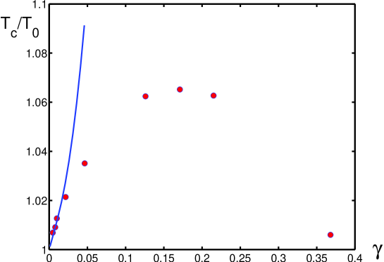
Figure 1: Relative critical temperature as a function of the gas parameter for a homogeneous system with $N=2$. Solid line corresponds to the asymptotic expression (4); dots are the Monte Carlo results from Table 5.

By Monte Carlo simulations, one can find the critical temperature not only for weak interactions, when the gas parameter is small, $\gamma\rightarrow 0$, but also for finite $\gamma$, as has been done by Pilati et al. [40] for $N=2$, whose results are presented in Table 5. In Fig. 1, we show the relative critical temperature of Bose-Einstein condensation $T_{c}/T_{0}$ as a function of the gas parameter $\gamma$, following from Eq. (4), as compared with the Monte Carlo results from Table 5. As is clear, Eq. (4) is valid only for $\gamma\rightarrow 0$, as one could expect. In the simulations of Pilati et al. [40], a Bose gas of hard spheres is considered, where $a_{s}$ corresponds to the hard-sphere diameter. The hard-sphere system is often used as a reference system for realistic fluids, such as liquid helium [41, 42]. When $a_{s}$ is much shorter than the mean interatomic distance $a$, the results for the local pseudopotential coincide with those for the hard-sphere system [43]. Moreover, the results for the local potential can be extended [44] to finite values of the ratio $a_{s}/a$ up to $a_{s}/a=0.65$, where the fluid freezes [45]. Generally, it is possible to show that pseudopotentials can be employed for a rather accurate modeling of physical systems, including those with nonintegrable interaction potentials [46]. In the case of superfluid ⁴He at saturated vapor pressure, the effective hard-sphere diameter is $a_{s}=2.203\AA$, which corresponds to the gas parameter $\gamma=0.5944$ and to the relative critical temperature $T_{c}/T_{0}=0.7$.

Notice that the critical temperature, at asymptotically weak interactions increases with $\gamma$. This is because an ideal homogeneous Bose-condensed gas is unstable, while interactions stabilize it [47, 48]. At the same time, strong interactions destroy the condensate, because of which at higher values of $\gamma$ the critical temperature diminishes.

3 Trapped Bose gas

Many finite quantum systems are well represented as being confined by effective potentials [49]. Most often, one considers a three-dimensional harmonic trapping potential

$$U({\bf r})=\frac{m}{2}\left(\omega_{x}^{2}x^{2}+\omega_{y}^{2}y^{2}+\omega_{z}^{2}z^{2}\right)\;.$$ (11)

Strictly speaking, genuine Bose-Einstein condensation happens only in an infinite system. For a gas confined by the harmonic potential, this implies [50] the limits

$$N\rightarrow\infty\;,\qquad\omega_{0}\rightarrow 0\;,\qquad N\omega_{0}^{3}\rightarrow const\;.$$ (12)

Here $N$ is the number of atoms in the trap and

$$\omega_{0}\equiv(\omega_{x}\omega_{y}\omega_{z})^{1/3}\;.$$ (13)

For finite $N$ there occurs pseudocondensation or quasicondensation [51], which in what follows, for short, will also be called condensation.

The ideal Bose gas in a harmonic trap condenses at the critical temperature

$$T_{0}=\left[\frac{N}{\zeta(3)}\right]^{1/3}\omega_{0}\;.$$ (14)

At this temperature, the thermal wavelength is

$$\lambda_{0}\equiv\sqrt{\frac{2\pi}{mT_{0}}}=\sqrt{\frac{2\pi}{m\omega_{0}}}\left[\frac{\zeta(3)}{N}\right]^{1/6}\;.$$ (15)

The ratio

$$\alpha\equiv\frac{a_{s}}{\lambda_{0}}$$ (16)

plays the role of a dimensionless coupling parameter. The critical temperature shift in terms of the asymptotically small parameter reads as [52]

$$\frac{\Delta T_{c}}{T_{0}}\simeq\overline{c}_{1}\alpha+\left(\overline{c}_{2}+\overline{c}_{2}^{\prime}\ln\alpha\right)\alpha^{2}\;.$$ (17)

The first coefficient is known [50, 51] from perturbative calculations, and the coefficient $\bar{c}_{2}^{\prime}$ can also be calculated perturbatively [52],

$$\overline{c}_{1}=-3.426032\;,\qquad\overline{c}_{2}^{\prime}=-\;\frac{32\pi\zeta(2)}{3\zeta(3)}=-45.856623\;.$$ (18)

The coefficient $\bar{c}_{2}$ can be related to lattice simulations in three-dimensional ${\mathcal{O}}(2)$ field theory [52],

$$\overline{c}_{2}=21.4-\;\frac{16\pi\zeta(2)}{3\zeta(3)}\;\left[\ln(32\pi^{3})+3.522272\right]+12\zeta(2)\left[\zeta\left(\frac{3}{2}\right)\right]^{4/3}d_{2}\;,$$ (19)

with the same $d_{2}$ as in Eq. (9). Using the Monte Carlo result [9] for $d_{2}$, one has

$$\overline{c}_{2}=-155.0\;.$$

We may notice the difference with the case of a homogeneous gas, where the linear term is positive, while for the trapped gas, according to Eq. (18), it is negative. This is because the ideal Bose-condensed gas in a three-dimensional harmonic trap is stable, so that switching on interactions immediately starts destroying the condensate. While, on the contrary, the ideal homogeneous Bose-condensed gas is unstable. Therefore interactions play the dual role, first stabilizing the system and then, when the interactions become sufficiently strong, they start depleting the condensate [5, 48].

The critical temperature shift due to repulsive interactions was studied experimentally for harmonically trapped ⁸⁷Rb atoms [53] and ³⁹K atoms [54, 55], varying the interaction strength by means of Feshbach resonance. The measurements were found to be in good agreement with the first coefficient $\bar{c}_{1}\approx-3.426$. However the next term was different, as compared with Eq. (17). Exploring the range $0.001<\alpha<0.06$, all experimental data points were fitted [54, 55] by the second-order polynomial

$$\frac{\Delta T_{c}}{T_{0}}=b_{1}\alpha+b_{2}\alpha^{2}\;,$$ (20)

with the coefficients

$$b_{1}=\overline{c}_{1}=-3.426\;,\qquad b_{2}=46\pm 5\;.$$

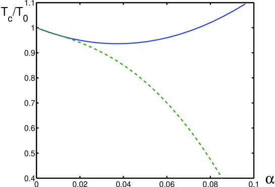
Figure 2: Relative critical temperature of Bose-Einstein condensation of trapped atoms, corresponding to Eq. (17) (dashed line) and to Eq. (20) (solid line), as a function of the coupling parameter $\alpha$.

The second-order positive term is due to atomic correlations beyond mean-field picture [56, 57, 58, 59, 60]. In order to show how expressions Eq. (17) and Eq. (20) are different, they are presented in Fig. 2.

4 Power-law traps

Traps, confining atoms, can be not only harmonic, but more generally, of power law, having in $d$-dimensional space the form

$$U({\bf r})=\sum_{\alpha=1}^{d}\frac{\omega_{\alpha}}{2}\left|\frac{r_{\alpha}}{l_{\alpha}}\right|^{n_{\alpha}}\qquad\left(l_{\alpha}\equiv\frac{1}{\sqrt{m\omega_{\alpha}}}\right)\;.$$ (21)

The characteristic trap frequency and length are defined as

$$\omega_{0}\equiv\left(\prod_{\alpha=1}^{d}\omega_{\alpha}\right)^{1/d}=\frac{1}{ml_{0}^{2}}\;,\qquad l_{0}\equiv\left(\prod_{\alpha=1}^{d}l_{\alpha}\right)^{1/d}=\frac{1}{\sqrt{m\omega_{0}}}\;,$$ (22)

respectively. For what follows, it is convenient to introduce the confining dimension [48, 61]

$$s\equiv\frac{d}{2}+\sum_{\alpha=1}^{d}\frac{1}{n_{\alpha}}\;.$$ (23)

Let us consider the ideal Bose gas trapped inside potential (21). In the semiclassical description, we have the density of states

$$\rho(\varepsilon)=\frac{\varepsilon^{s-1}}{\gamma_{d}\Gamma(s)}\qquad\left(s\geq\frac{1}{2}\right)\;,$$ (24)

in which

$$\gamma_{d}\equiv\frac{\pi^{d/2}}{2^{s}}\prod_{\alpha=1}^{d}\frac{\omega_{\alpha}^{1/2+1/n_{\alpha}}}{\Gamma(1+1/n_{\alpha})}\qquad(d\geq 1)\;.$$ (25)

In the standard semiclassical approximation, the energy variable $\varepsilon$ varies between zero and infinity, as a result of which Bose condensation becomes impossible in some low-dimensional traps [62, 63, 64]. However, in quantum systems the energy varies not from zero, but from a finite value $\varepsilon_{0}$ corresponding to the lowest energy level of the quantum system. By the order of magnitude, it is possible to approximate the minimal energy as

$$\varepsilon_{0}\approx\frac{k_{min}^{2}}{2m}\approx\frac{1}{2ml_{0}^{2}}=\frac{\omega_{0}}{2}\;.$$

Therefore the range of variation of $\varepsilon$ has to be

$$\varepsilon_{0}\approx\frac{\omega_{0}}{2}\leq\varepsilon<\infty\;.$$ (26)

Taking this into account defines the modified semiclassical approximation [61]. Then the Bose-Einstein function is modified to the form

$$g_{n}(z)=\frac{1}{\Gamma(n)}\int_{u_{min}}^{\infty}\frac{zu^{n-1}}{e^{u}-z}\;du\;,$$ (27)

where $z=e^{\beta\mu}$ is fugacity and the integration is not from zero, but from the finite lower limit

$$u_{min}\equiv\frac{\omega_{0}}{2T}\;.$$

The value $\omega_{0}/T_{0}$, where $T_{0}$ is the critical temperature of trapped ideal gas, is assumed to be small.

Bose-Einstein condensation of ideal gas in a power-law trap occurs (see details in Refs. [48, 61]) at the temperature

$$T_{0}=\left[\frac{\gamma_{d}N}{g_{s}(1)}\right]^{1/s}\;.$$ (28)

In particular, the condensation temperature formally exists in one-dimensional space, where for an anharmonic trap one has

$$T_{0}=\frac{\sqrt{\pi}(1-s)\Gamma(s)}{2\Gamma(1+1/n)}\;N\omega_{0}\qquad(d=1,\;s<1,\;n>2)\;.$$ (29)

For harmonic confinement, we come to the expression that coincides with that obtained in purely quantum consideration [65],

$$T_{0}=\frac{N\omega_{0}}{\ln(2N)}\qquad(s=d=1,\;n=2)\;.$$ (30)

And for two- and three-dimensional harmonic traps, we have

$$T_{0}=\omega_{0}\left[\frac{N}{\zeta(d)}\right]^{1/d}\qquad(s=d\geq 2,\;n_{\alpha}=2)\;.$$ (31)

Recall that Bose-Einstein condensation, strictly speaking, assumes thermodynamic limit, which requires to study the system properties under a large number of atoms. Usually, in traps this number is really large. In the presence of confining potentials, thermodynamic limit is defined differently as compared to homogeneous systems.

The most general definition of thermodynamic limit, valid for any system, is as follows [47, 48]: Extensive observable quantities $A_{N}$ must increase together with the number of particles $N$, so that

$$N\rightarrow\infty\;,\qquad A_{N}\rightarrow\infty\;,\qquad\frac{A_{N}}{N}\rightarrow const\;.$$ (32)

As an observable, it is possible to take the system energy $E_{N}$, so that

$$N\rightarrow\infty\;,\qquad E_{N}\rightarrow\infty\;,\qquad\frac{E_{N}}{N}\rightarrow const\;.$$ (33)

For the considered case, the latter reduces to the limit

$$N\rightarrow\infty\;,\qquad\gamma_{d}\rightarrow 0\;,\qquad N\gamma_{d}\rightarrow const\;.$$

In particular, for unipower potentials, when $n_{\alpha}=n$, we have

$$N\rightarrow\infty\;,\qquad\omega_{0}\rightarrow 0\;,\qquad N\omega_{0}^{s}\rightarrow const\;.$$ (34)

In this limit, the critical temperature (28), depending on the confining dimension $s$, behaves as

$$T_{0}\;\propto\;\frac{1}{N^{1/s-1}}\rightarrow 0\qquad(s<1)\;,$$

$$T_{0}\;\propto\;\frac{1}{\ln N}\rightarrow 0\qquad(s=1)\;,$$

$$T_{0}\;\propto\;const\qquad(s>1)\;.$$ (35)

This tells us that a well defined condensation temperature exists only for $s>1$.

Moreover, a critical temperature may formally exist, but the system below this temperature looses its stability, which implies that, actually, such a system cannot exist. To check the stability of a Bose-condensed system, we need to study its compressibility

$$\kappa_{T}=\frac{{\rm var}(\hat{N})}{\rho TN}=\frac{1}{\rho^{2}}\left(\frac{\partial\rho}{\partial\mu}\right)=\frac{1}{\rho N}\left(\frac{\partial N}{\partial\mu}\right)\;,$$ (36)

in which $\hat{N}$ is the number-of-particle operator and

$${\rm var}(\hat{N})\equiv\langle\hat{N}^{2}\rangle-\langle\hat{N}\rangle^{2}\;.$$

An equilibrium system is stable provided that its particle fluctuations are thermodynamically normal [47, 66, 67], such that

$$0\leq\kappa_{T}<\infty\;.$$ (37)

In other words, the stability condition is

$$0\leq\frac{{\rm var}(\hat{N})}{N}<\infty\;.$$ (38)

Calculating the compressibility, we find that, above the condensation phase transition, systems with the confining dimension $s<1$ are unstable, since

$$\kappa_{T}\;\propto\;-N^{1/s-1}\rightarrow-\infty\qquad(s<1,\;T>T_{0})\;.$$ (39)

While for larger confining dimensions, systems are stable,

$$\kappa_{T}\;\propto\;const\qquad(s\geq 1,\;T>T_{0})\;.$$ (40)

The situation is even more delicate below the transition temperature $T_{0}$, where the systems up to $s=2$ are unstable, with

$$\kappa_{T}\;\propto\;-N^{2/s-1}\rightarrow-\infty\qquad(s<1)\;,$$

$$\kappa_{T}\;\propto\;N\rightarrow\infty\qquad(s=1)\;,$$

$$\kappa_{T}\;\propto\;N^{2/s-1}\rightarrow\infty\qquad(1<s<2)\;,$$

$$\kappa_{T}\;\propto\;\ln N\rightarrow\infty\qquad(s=2)\;.$$ (41)

And only for larger $s>2$, they are stable, because

$$\kappa_{T}\;\propto\;const\qquad(s>2)\;.$$ (42)

Remembering the definition of the confining dimension (23), we find the stability condition

$$\frac{d}{2}+\sum_{\alpha=1}^{d}\frac{1}{n_{\alpha}}>2\;.$$ (43)

For harmonic confinement, when $n_{\alpha}=2$, we have

$$s=d\qquad(n_{\alpha}=2)\;.$$

Then we see that Bose-condensed systems in one- and two-dimensional harmonic traps are unstable, displaying thermodynamically anomalous particle fluctuations,

$$\kappa_{T}\;\propto\;N\rightarrow\infty\qquad(s=d=1)\;,$$

$$\kappa_{T}\;\propto\;\ln N\rightarrow\infty\qquad(s=d=2)\;.$$ (44)

And only a three-dimensional harmonic trap can confine a stable Bose-condensed system, with a finite compressibility,

$$\kappa_{T}\;\propto\;const\qquad(s=d=3)\;.$$ (45)

Although Bose-condensed gas is unstable in one- and two-dimensional harmonic traps, it can be stable for other powers of the confining potential. As an example, let us consider the unipower potentials, when $n_{\alpha}=n$. Then the confining dimension is

$$s=\left(\frac{1}{2}+\frac{1}{n}\right)d\;.$$

According to condition (43), the ideal Bose-condensed gas is stable if the confining dimension $s>2$. Therefore, the gas is stable in different real-space dimensions $d$, provided that the potential powers $n$ are limited from above:

$$n<\frac{2d}{4-d}\;.$$

That is,

$$n<\frac{2}{3}\qquad(d=1)\;,$$

$$n<2\qquad(d=2)\;,$$

$$n<6\qquad(d=3)\;.$$

The existence of the upper potential power $n$ for stability can be understood, if one remembers that the passage from a trapped gas to the uniform gas confined in a box of length $L$ corresponds to the limits

$$n\rightarrow\infty\;,\qquad l_{0}\rightarrow\frac{L}{2}\;,\qquad s\rightarrow\frac{d}{2}\;.$$

Hence increasing $n$ approaches the system to the uniform case that is known to be unstable [47, 48].

Generally, for stability of a system, it is also necessary that thermal fluctuations be thermodynamically normal [47]. Calculating specific heat, we find [48, 61] that it is positive and finite for all $s\geq 1/2$. From the definition of the confining dimension $s$ it follows that it is always not smaller than $1/2$. Hence thermal fluctuations are thermodynamically normal for the considered trapped systems. And stability is defined by the behavior of the isothermal compressibility.

5 Finite-size corrections

Describing Bose gas in power-law traps, we have used the modified semiclassical approximation, accepting the modified function

$$g_{s}(z)=\frac{1}{\Gamma(s)}\int_{\beta\varepsilon_{0}}^{\infty}\;\frac{zu^{s-1}}{e^{u}-z}\;du\;,$$ (46)

with a finite lower integration limit, instead of the usual Bose-Einstein function

$$g_{s}^{(0)}(z)=\frac{1}{\Gamma(s)}\int_{0}^{\infty}\frac{zu^{s-1}}{e^{u}-z}\;du\;,$$ (47)

with the zero lower limit. In the modified variant, the transition temperature is given by Eq. (28), while in the standard case, taking into account that $g^{(0)}_{s}(1)=\zeta(s)$, it is

$$T_{0}^{(0)}=\left[\frac{\gamma_{d}N}{\zeta(s)}\right]^{1/s}\qquad(s>1)\;.$$ (48)

A finite positive value for the latter temperature exists only for $s>1$, since the Rieman zeta function $\zeta(s)$ is finite and positive for $s>1$, finite but negative for $0\leq s<1$, and infinite at $s=1$, where $\zeta(s)\rightarrow+\infty$, as $s\rightarrow 1+0$.

In order to study how the use of the modified function (46) influences the value of the transition temperature, let us consider the critical temperature shift under a large number of atoms,

$$\frac{\Delta T_{0}}{T_{0}^{(0)}}\equiv\frac{T_{0}-T_{0}^{(0)}}{T_{0}^{(0)}}\;,$$

where $s>1$, since finite temperature (48) exists only for this confining dimension. We find [48]

$$\frac{\Delta T_{0}}{T_{0}^{(0)}}=\frac{1}{s(s-1)\Gamma(s)\zeta(s)}\left(\frac{\varepsilon_{0}}{T_{0}}\right)^{s-1}\;,$$ (49)

which shows that at large $N$ one has

$$\frac{\Delta T_{0}}{T_{0}^{(0)}}\;\propto\;\frac{1}{N^{1-1/s}}\qquad(s>1)\;.$$

For harmonic traps, it follows

$$\frac{\Delta T_{0}}{T_{0}^{(0)}}=\frac{1}{4\sqrt{\zeta(2)}\;N^{1/2}}\qquad(s=d=2)\;,$$

$$\frac{\Delta T_{0}}{T_{0}^{(0)}}=\frac{1}{48[\zeta(3)]^{1/3}\;N^{2/3}}\qquad(s=d=3)\;.$$ (50)

The found critical temperature shifts represent finite-size corrections related to the quantum nature of trapped atomic systems. A finite quantum system possesses an energy spectrum with a nonzero energy $\varepsilon_{0}$ of the lowest level. This has been taken into account in modifying function (47) to (46). However, the quantum nature of trapped systems also plays the role in a different, and even more important, way, as is shown in the following section.

6 Quantum corrections

As far as a finite quantum system possesses a spectrum with a nonzero lowest energy level $\varepsilon_{0}$, then at the Bose-Einstein condensation temperature $T_{c}$, the chemical potential tends to $\varepsilon_{0}$, but not to zero. Therefore the fugacity $z=\exp(\beta\mu)$ tends to $\exp(\varepsilon_{0}/T_{c})$, but not to one.

In the previous section, we considered how the critical temperature varies when $g_{s}^{(0)}(1)$ is replaced by $g_{s}(1)$. Now, our aim is to study the variation of the critical temperature under the replacement of $g_{s}^{(0)}(1)$ by $g_{s}^{(0)}(e^{\beta\varepsilon_{0}})$. Similarly to the previous section, we consider the confining dimensions $s>1$.

Let us denote by $T_{c}$ the critical temperature calculated with the use of $g_{s}^{(0)}(e^{\beta\varepsilon_{0}})$ and by $T_{0}$ the condensation temperature corresponding to $g_{s}^{(0)}(1)$. For the relative critical temperature shift, we find [48]

$$\frac{\Delta T_{c}}{T_{0}}=-\;\frac{(s-1)\varepsilon_{0}}{s(2-s)\Gamma(s)\zeta(s)T_{0}}\left(\frac{T_{0}}{\varepsilon_{0}}\right)^{2-s}\qquad(1<s<2)\;,$$

$$\frac{\Delta T_{c}}{T_{0}}=-\;\frac{\varepsilon_{0}}{2\zeta(2)T_{0}}\;\ln\left(\frac{T_{0}}{\varepsilon_{0}}\right)\qquad(s=2)\;,$$

$$\frac{\Delta T_{c}}{T_{0}}=-\;\frac{\zeta(s-1)\varepsilon_{0}}{s\zeta(s)T_{0}}\qquad(s>2)\;.$$ (51)

Taking into account that $\varepsilon_{0}$ varies with increasing $N$ in the same way as $\omega_{0}$, that is $\varepsilon_{0}\propto N^{-1/s}$, one finds

$$\frac{\Delta T_{c}}{T_{0}}\;\propto\;-\;\frac{1}{N^{1-1/s}}\qquad(1<s<2)\;,$$

$$\frac{\Delta T_{c}}{T_{0}}\;\propto\;-\;\frac{\ln N}{\sqrt{N}}\qquad(s=2)\;,$$

$$\frac{\Delta T_{c}}{T_{0}}\;\propto\;-\;\frac{1}{N^{1/s}}\qquad(s>2)\;.$$ (52)

As is seen, the corrections here are of different sign as compared to the previous section. They are of the same order of magnitude for $1<s<2$, but

$$\left|\frac{\Delta T_{c}}{T_{0}}\right|\gg\frac{\Delta T_{0}}{T_{0}^{(0)}}\qquad(s\geq 2,\;N\rightarrow\infty)$$ (53)

for large $N$. Remembering that the ideal Bose-condensed gas is stable only for $s>2$, we come to the conclusion that, for stable systems, the quantum corrections to the critical temperature, found in the present section, are more important than those of the previous section.

For a three-dimensional harmonic trapping potential, one finds [68, 69].

$$\frac{\Delta T_{c}}{T_{0}}=-\;\frac{\zeta(2)\overline{\omega}}{2[\zeta(3)]^{2/3}\omega_{0}N^{1/3}}\qquad(s=d=3)\;,$$ (54)

with the notation for the average trap frequency

$$\overline{\omega}\equiv\frac{1}{d}\sum_{\alpha=1}^{d}\omega_{\alpha}\;.$$

This can be rewritten as

$$\frac{\Delta T_{c}}{T_{0}}=-0.727504\left(\frac{\overline{\omega}}{\omega_{0}}\right)\frac{1}{N^{1/3}}\;.$$ (55)

For anisotropic traps, $\bar{\omega}>\omega_{0}$. And in the case of a spherical harmonic trap, $\bar{\omega}=\omega_{0}$.

7 Interaction corrections

The semiclassical approximation can also be used for calculating the critical temperature shift under switching on weak interactions of atoms trapped in a harmonic potential. Above the critical temperature, the spectrum of atoms interacting through the local potential

$$\Phi({\bf r})=\Phi_{0}\delta({\bf r})\qquad\left(\Phi_{0}\equiv 4\pi\;\frac{a_{s}}{m}\right)\;,$$

in the semiclassical approximation, is

$$\varepsilon_{k}({\bf r})=\frac{k^{2}}{2m}+U({\bf r})+2\Phi_{0}\rho({\bf r})\qquad(T>T_{c})\;,$$ (56)

where $\rho({\bf r})$ is the local density of atoms. At the critical point, the chemical potential behaves as

$$\mu\rightarrow 2\Phi_{0}\rho(0)\qquad(T\rightarrow T_{c}+0)\;.$$ (57)

It is possible to show [48] that the interaction corrections can be small only for $s>2$ and $d>2$. Therefore in what follows, we take $d=3$ and assume that $s>2$, which yields

$$\frac{\Delta T_{c}}{T_{0}}=-c_{3}(s)\;\frac{a_{s}}{\lambda_{0}}\qquad(s>2)\;,$$ (58)

with the thermal length

$$\lambda_{0}\equiv\sqrt{\frac{2\pi}{mT_{0}}}=\sqrt{2\pi}\;[\zeta(3)]^{1/6}\frac{l_{0}}{N^{1/6}}\;,$$ (59)

and with the notation

$$c_{3}(s)\equiv\frac{4}{s\zeta(s)}\left[\zeta\left(\frac{3}{2}\right)\zeta(s-1)-S_{3}(s)\right]\;,\qquad S_{3}(s)\equiv\sum_{m,n=1}^{\infty}\frac{n}{(mn)^{3/2}(m+n)^{s-3/2}}\;.$$

For a harmonic trap, when $s=d=3$, one gets [50].

$$\frac{\Delta T_{c}}{T_{0}}=-3.426032\;\frac{a_{s}}{\lambda_{0}}\;.$$ (60)

This reproduces the linear term in expansion (17).

In the similar way, it is possible to find the critical temperature shift for other types of interaction potentials, for instance for dipolar interactions [70, 71, 72], for which the shift

$$\frac{\Delta T_{c}}{T_{0}}\;\propto\;\frac{a_{D}}{\lambda_{0}}$$

is proportional to the dipolar length $a_{D}\equiv md_{0}^{2}$, with $d_{0}$ being dipolar moment.

Note that in the effective thermodynamic limit (34) we have $\gamma_{d}\propto\omega_{0}^{s}$ and $\omega_{0}\propto N^{-1/s}$. For a three-dimensional trap $s=d=3$, hence $\omega_{0}\propto N^{-1/3}$. Then $l_{0}\propto N^{1/6}$, while $\lambda_{0}\propto const$.

8 Box-shaped trap

Quasi-uniform traps of box shape have recently become available [73]. If the trap has the shape of a box of linear length $L$ and volume $V=L^{3}$, then the atomic wave function has to satisfy the boundary conditions

$$\psi(r_{x},r_{y},r_{z})=0\qquad(r_{\alpha}=0,L)\;.$$ (61)

The finite size of the box makes the condensation temperature $T_{c}$ different from the transition temperature $T_{0}$ of an infinite homogeneous system. In the case of ideal gas,

$$T_{0}=\frac{2\pi}{m}\left[\frac{\rho}{\zeta(3/2)}\right]^{2/3}\qquad(V\rightarrow\infty)\;.$$ (62)

For the ideal gas, the shift of the critical temperature, caused by the finite size of the box, reads as [74]

$$\frac{\Delta T_{c}}{T_{0}}=0.351467\;\frac{\ln N}{N^{1/3}}\;.$$ (63)

However, if the box is strictly rectangular, and the Bose gas is ideal, then its condensation makes the system unstable, because of thermodynamically anomalous fluctuations, similarly to the homogeneous ideal Bose gas. This follows [48] from the number-of-particle variance

$${\rm var}(\hat{N})=\frac{0.423}{2\pi^{3}}\;(mT)^{2}V^{4/3}$$ (64)

yielding the anomalous isothermal compressibility

$$\kappa_{T}=0.00682\;\frac{m^{2}T}{\rho^{7/3}}\;N^{1/3}\;.$$ (65)

The ideal Bose-condensed gas is unstable either in an infinite homogeneous system or in a finite box-shaped trap. Fortunately, real atomic systems always enjoy interactions that can stabilize the Bose-condensed gas.

9 Optical lattices

Cold atoms can be loaded in different optical lattices created by laser beams [75, 76, 77, 78]. The standard periodic potential, formed by the beams, reads as

$$V_{L}({\bf r})=\sum_{\alpha=1}^{d}V_{\alpha}\sin^{2}\left(k_{0}^{\alpha}r_{\alpha}\right)\;,$$ (66)

where ${\bf k_{0}}$ is the laser wave vector,

$$k_{0}^{\alpha}\equiv\frac{2\pi}{\lambda_{\alpha}}=\frac{\pi}{a_{\alpha}},$$

$\lambda_{\alpha}$ is a laser wavelength, and $a_{\alpha}$ is a lattice spacing in the $\alpha$-direction. The lattice depth, or barrier, is characterized by the quantity

$$V_{0}\equiv\frac{1}{d}\sum_{\alpha=1}^{d}V_{\alpha}\;.$$ (67)

Atoms, subject to the action of the laser beams, have the recoil energy

$$E_{R}\equiv\frac{k_{0}^{2}}{2m}\qquad\left(k_{0}^{2}=\sum_{\alpha=1}^{d}(k_{0}^{\alpha})^{2}\right)\;.$$ (68)

The atomic field operator can be expanded over Wannier functions that can be chosen to be well localized [79],

$$\hat{\psi}({\bf r})=\sum_{jn}\hat{c}_{jn}w_{n}({\bf r}-{\bf a}_{j})\;,$$ (69)

here $j=1,2,\ldots N_{L}$ enumerates the lattice sites and $n$ is a band index. Substituting this expansion into the Hamiltonian, one usually considers only the lowest energy band. Then, keeping in mind local interactions, characterized by the scattering length $a_{s}$, yields the Hubbard Hamiltonian

$$\hat{H}=-J\sum_{\langle ij\rangle}\hat{c}_{i}^{\dagger}\hat{c}_{j}\;+\;\frac{U}{2}\sum_{j}\hat{c}_{j}^{\dagger}\hat{c}_{j}^{\dagger}\hat{c}_{j}\hat{c}_{j}\;+\;h_{0}\sum_{j}\hat{c}_{j}^{\dagger}\hat{c}_{j}\;.$$ (70)

The Hamiltonian parameters in three dimensions, resorting to the tight-binding approximation, can be presented [78] as follows. The tunneling parameter reads as

$$J=\frac{3}{4}\left(\pi^{2}-4\right)V_{0}\exp\left(-\;\frac{3\pi^{2}}{4}\;\sqrt{\frac{V_{0}}{E_{R}}}\right)\;.$$ (71)

The on-site interaction is described by

$$U=\sqrt{\frac{8}{\pi}}\;k_{0}a_{s}E_{R}\left(\frac{V_{0}}{E_{R}}\right)^{3/4}\;.$$ (72)

And the last term contains

$$h_{0}=3E_{R}\;\sqrt{\frac{V_{0}}{E_{R}}}\;.$$ (73)

In the presence of Bose-Einstein condensate, global gauge symmetry is broken, which is the necessary and sufficient condition for the condensation [80, 81, 82]. The most convenient way for breaking the symmetry is through the Bogolubov shift that here is equivalent to the canonical transformation

$$\hat{c}_{j}=\sqrt{\nu n_{0}}\;+\;c_{j}\;,$$ (74)

in which $\nu$ is the lattice filling factor

$$\nu\equiv\frac{N}{N_{L}}=\rho a^{d}\;,$$ (75)

where $\rho$ is average atomic density, $a$ is a mean interatomic distance, and $n_{0}=N_{0}/N$ is the condensate fraction.

The operator of uncondensed atoms satisfies [78] the properties

$$\langle c_{j}\rangle=0\;,\qquad\sum_{j}c_{j}=0\;.$$ (76)

In the Hartree-Fock-Bogolubov approximation, the critical temperature of Bose-Einstein condensation, in $d$ dimensions, becomes [78, 83]

$$T_{c}=4\pi\;\frac{d-2}{d}\left[\Gamma\left(1+\frac{d}{2}\right)\right]^{2/d}J\nu\;.$$ (77)

In three dimensions, this reduces to

$$T_{c}=5.064222J\nu\;.$$ (78)

In view of the tunneling parameter (71), we have

$$\frac{T_{c}}{\nu E_{R}}=22.294\;\frac{V_{0}}{E_{R}}\;\exp\left(-\;\frac{3\pi^{2}}{4}\;\sqrt{\frac{V_{0}}{E_{R}}}\right)\;.$$ (79)

Recall that this expression is valid in the tight-binding approximation, when $E_{R}\ll V_{0}$.

The dependence of the critical temperature on the lattice and interaction parameters was studied by Monte Carlo simulations [84]. The linear variation of $T_{c}$ with the filling factor, agreeing with Eq. (78), is confirmed for $\nu<6$.

Particle fluctuations in the lattice are thermodynamically normal, with the atomic variance

$${\rm var}(\hat{N})=\frac{NT}{\nu U(n_{0}+\sigma)}\;,$$

where

$$\sigma=\frac{1}{N}\sum_{j}\langle c_{j}c_{j}\rangle$$

is the anomalous average. This gives the isothermal compressibility

$$\kappa_{T}=\frac{{\rm var}(\hat{N})}{\rho TN}=\frac{1}{\rho\nu(n_{0}+\sigma)U}\;.$$ (80)

As is seen, if the interaction parameter $U$ tends to zero, then the compressibility diverges, which means that the ideal Bose-condensed gas in a lattice is unstable, while repulsive interactions stabilize it.

Taking into account intersite atomic interactions results in the extended Hubbard model

$$\hat{H}=-J\sum_{\langle ij\rangle}\hat{c}_{i}^{\dagger}\hat{c}_{j}\;+\;\frac{U}{2}\sum_{j}\hat{c}_{j}^{\dagger}\hat{c}_{j}^{\dagger}\hat{c}_{j}\hat{c}_{j}\;+\;\frac{1}{2}\sum_{i\neq j}U_{ij}\hat{c}_{i}^{\dagger}\hat{c}_{j}^{\dagger}\hat{c}_{i}\hat{c}_{j}\;+\;h_{0}\sum_{j}\hat{c}_{j}^{\dagger}\hat{c}_{j}\;.$$

This model is usually studied by means of numerical calculations, such as density-matrix renormalization group [85, 86] and quantum Monte Carlo simulations [87, 88, 89]. In the presence of intersite interactions collective phonon excitations arise, which can make an optical lattice unstable although long living [90].

10 Conclusion

The critical temperature of Bose-Einstein condensation is one of the main characteristics of Bose systems. In the present brief review, we give a survey of critical temperatures for typical systems experiencing Bose-Einstein condensation. These are weakly interacting uniform Bose gases, trapped Bose gases confined in power-law potentials, and bosons in optical lattices. The emphasis is on the cases allowing for the derivation of explicit expressions for the critical temperature. Such explicit expressions, even being approximate, make it possible to better understand the dependence of the temperature on system parameters and to estimate optimal conditions for realizing Bose-Einstein condensation.

In the process of calculating a critical temperature, it is often necessary to employ elaborate mathematical methods. One such a very powerful method is based on self-similar approximation theory. Since this approach can be useful for calculating the critical temperature of different systems, it is sketched in the Appendix.

Appendix. Self-similar factor approximants

In many cases, the considered system is rather complicated allowing only for the use of some kind of perturbation theory in powers of an asymptotically small parameter, while in real physical systems this parameter can be finite or even very large.

Suppose we are interested in a function $f(x)$ of a real variable $x$, for which one can get an expansion in powers of this variable, obtaining

$$f(x)\simeq f_{k}(x)\qquad(x\rightarrow 0)\;,$$

with

$$f_{k}(x)=f_{0}(x)\left(1+\sum_{n=1}^{k}a_{n}x^{n}\right)\;,$$

where $f_{0}(x)$ is given. And assume that we need to know the value of the function for finite, or even large, variable $x$. That is, we need a method of extrapolating the function from asymptotically small $x$ to the region of finite $x$. A very powerful and rather simple method is based on self-similar approximation theory [27, 28, 29, 30, 31, 32, 33]. Here we briefly mention the main ideas of the theory and its particular approach of extrapolation by self-similar factor approximants [34, 35, 36].

A finite series can be treated as a polynomial. By the fundamental theorem of algebra, a polynomial

$$P_{k}(z)=\sum_{n=0}^{k}a_{n}z^{n}$$

over the field of complex numbers (generally, with $a_{n}$ and $z$ complex-valued) can be uniquely presented as the product

$$P_{k}(z)=\prod_{j=1}^{k}(a_{j}+b_{j}z)\;.$$

Therefore, we can write

$$\left(1+\sum_{n=1}^{k}a_{n}x^{n}\right)=\prod_{j=1}^{k}(1+b_{j}x)\;.$$

The self-similar transformation of the linear function gives [34, 35, 36].

$$(1+b_{j}x)\rightarrow(1+A_{j}x)^{n_{j}}\;.$$

Then the series $f_{k}(x)$ transforms to the self-similar factor approximant

$$f_{k}^{*}(x)=f_{0}(x)\prod_{j=1}^{N_{k}}(1+A_{j}x)^{n_{j}}\;,$$

where $N_{k}$ will be given below and the parameters $A_{j}$ and $n_{j}$ are defined by the accuracy-through-order procedure, that is, by equating the like-order terms in the small-variable expansion, so that

$$f_{k}^{*}(x)\simeq f_{k}(x)\qquad(x\rightarrow 0)\;.$$

If the order $k$ is even, then $N_{k}=k/2$. And the accuracy-through-order procedure yields $k$ equations

$$\sum_{j=1}^{k/2}n_{j}A_{j}^{n}=D_{n}\qquad(n=1,2,\ldots,k)\;,$$

in which

$$D_{n}\equiv\frac{(-1)^{n-1}}{(n-1)!}\;\lim_{x\rightarrow 0}\;\frac{d^{n}}{dx^{n}}\;\ln\left(1+\sum_{m=1}^{n}a_{m}x^{m}\right)\;.$$

For instance,

$$D_{1}=a_{1}\;,\qquad D_{2}=a_{1}^{2}-2a_{2}\;,\qquad D_{3}=a_{1}^{3}-3a_{1}a_{2}+3a_{3}\;.$$

In these equations, there are $k/2$ unknown $A_{j}$ and $k/2$ unknown $n_{j}$, so that the total number of unknowns equals the number of equations.

If $k$ is odd, then we may set $N_{k}=(k+1)/2$. However, then we again get $k$ equations

$$\sum_{j=1}^{(k+1)/2}n_{j}A_{j}^{n}=D_{n}\qquad(n=1,2,\ldots,k)\;,$$

but now with $(k+1)/2$ unknown $A_{j}$ and $(k+1)/2$ unknown $n_{j}$, which makes $k+1$ unknowns. One of the parameters remains undefined, requiring to impose an additional condition. It is possible to resort to the scaling condition [36], agreeing to measure the parameters $A_{j}$ in units of one of them, say $A_{1}$. This is equivalent to setting $A_{1}=1$. Thus

$$N_{k}=\left\{\begin{array}[]{ll}k/2\;,{}{}&~{}~{}k=2,4,\ldots\\ (k+1)/2\;,{}{}&~{}~{}k=3,5,\ldots\end{array}\right.\;,$$ (83)

with the scaling condition $A_{1}=1$ for odd $k$.

The accuracy-through-order equations with respect to $A_{j}$ are polynomial, the first equation being of first order, the second, of second order, and so on, with the last equation being of order $k$. Each polynomial equation of order $n$ possesses $n$ solutions. So that the total number of solutions is $1\times 2\times 3\cdots\times k=k!$. At the same time, from the form of the factor approximants it is evident that each of them is invariant with respect to the $k!$ permutations

$$A_{i}\rightarrow A_{j}\;,\qquad n_{i}\rightarrow n_{j}\;.$$

Therefore, the multiplicity of solutions for $A_{j}$ is trivial, being related to the enumeration of the parameters. Up to this enumeration, the solutions are unique.

If the parameters $A_{j}$ are given, then we get the linear algebraic equations with respect to $n_{j}$. The solutions for the latter have the form

$$n_{j}=\frac{U_{j}(N_{k})}{V(N_{k})}\qquad(j=1,2,\ldots,N_{k})\;.$$

Here the nominator is the determinant

$$U_{j}(N_{k})=\left|\begin{array}[]{cccccc}A_{1}&A_{2}&\ldots&D_{1}&\ldots&A_{N_{k}}\\ A_{1}^{2}&A_{2}^{2}&\ldots&D_{2}&\ldots&A_{N_{k}}^{2}\\ \ldots&\ldots&\ldots&\ldots&\ldots&\ldots\\ A_{1}^{N_{k}}&A_{2}^{N_{k}}&\ldots&D_{N_{k}}&\ldots&A_{N_{k}}^{N_{k}}\end{array}\right|\;,$$ (88)

with $D_{i}$ in the $j$-th column, and the denominator is the Vandermonde-Knuth determinant

$$V(N_{k})=\left|\begin{array}[]{cccccc}A_{1}&A_{2}&\ldots&A_{j}&\ldots&A_{N_{k}}\\ A_{1}^{2}&A_{2}^{2}&\ldots&A_{j}^{2}&\ldots&A_{N_{k}}^{2}\\ \ldots&\ldots&\ldots&\ldots&\ldots&\ldots\\ A_{1}^{N_{k}}&A_{2}^{N_{k}}&\ldots&A_{j}^{N_{k}}&\ldots&A_{N_{k}}^{N_{k}}\end{array}\right|\;.$$ (93)

When $k$ is odd, hence $A_{1}=1$, then $V(N_{k})$ is the standard Vandermonde determinant, while when $k$ is even, this determinant by the relation

$$V(N_{k})=\left(\prod_{j=1}^{N_{k}}A_{j}\right)\overline{V}(N_{k})$$

is connected with the Vandermonde determinant

$$\overline{V}(N_{k})=\left|\begin{array}[]{cccccc}1&1&\ldots&1&\ldots&1\\ A_{1}&A_{2}&\ldots&A_{j}&\ldots&A_{N_{k}}\\ A_{1}^{2}&A_{2}^{2}&\ldots&A_{j}^{2}&\ldots&A_{N_{k}}^{2}\\ \ldots&\ldots&\ldots&\ldots&\ldots&\ldots\\ A_{1}^{N_{k}-1}&A_{2}^{N_{k}-1}&\ldots&A_{j}^{N_{k}-1}&\ldots&A_{N_{k}}^{N_{k}-1}\end{array}\right|=\prod_{1\leq i<j\leq N_{k}}(A_{j}-A_{i})\;.$$ (99)

The beauty of the factor approximants is that they, in a finite order, can exactly reconstruct a large class of functions from their asymptotic expansions. This class includes rational, irrational, as well as transcendental functions [34, 35, 36]. For example, exactly reproducible are all functions of the type

$$R(x)=\prod_{j=1}^{M}P_{m_{j}}^{\alpha_{j}}(x)\;,$$

where $P_{m}(x)$ are polynomials and $\alpha_{j}$ are complex-valued numbers. To exactly reconstruct this function, one needs a factor approximant of the order

$$k=\sum_{j=1}^{M}m_{j}\;.$$

Exactly reproducible are transcendental functions that can be defined as limits of polynomials [36]. For instance, as is easy to check, since

$$\lim_{a\rightarrow 0}P_{1}^{1/a}(x)=e^{x}\qquad(P_{1}(x)=1+ax)\;,$$

the exponential function is exactly reproduced in any order $k\geq 2$. Keeping in mind such limits, the class of exactly reproducible functions can be denoted as

$${\cal R}=\{R(x),\;\lim R(x)\}\;.$$

Self-similar factor approximants extrapolate asymptotic series to finite values of the variables, and even to the variables tending to infinity. Thus, assuming that

$$f_{0}(x)\simeq Ax^{\alpha}\qquad(x\rightarrow\infty)\;,$$

we get the large-variable behavior of the factor approximant as

$$f_{k}^{*}(x)\simeq B_{k}x^{\beta}_{k}\qquad(x\rightarrow\infty)\;,$$

with the amplitude

$$B_{k}=A\prod_{j=1}^{N_{k}}A_{j}^{n_{j}}$$

and the power

$$\beta_{k}=\alpha+\sum_{j=1}^{N_{k}}n_{j}\;.$$

When the large-variable behavior of the sought function is known, say

$$f(x)\simeq Bx^{\beta}\qquad(x\rightarrow\infty)\;,$$

then it is possible to require that $\beta_{k}$ be equal to $\beta$,

$$\alpha+\sum_{j=1}^{N_{k}}n_{j}=\beta\;.$$

If it is known that the limit of the sought function is finite, hence $\beta=0$, then one has the condition

$$\alpha+\sum_{j=1}^{N_{k}}n_{j}=0\qquad(\beta=0)\;.$$

Thus, for a finite series $f_{k}(x)$, one gets a sequence $\{f_{n}^{*}(x)\}$ of self-similar factor approximants, with $n=1,2,\ldots k$. If the sequence converges numerically, then as the final answer one can accept the expression $[f_{k}^{*}(x)+f_{k-1}^{*}(x)]/2$, with the error bar $\pm|f_{k}^{*}(x)-f_{k-1}^{*}(x)|/2$.

The convergence of the sequence $\{f_{n}^{*}(x)\}$ can be accelerated in the following way. Being based on the last three factor approximants, one constructs a quadratic spline

$$q(x,t)=a(x)+b(x)t+c(x)t^{2}\;,$$

whose coefficients are determined from the conditions

$$q(x,0)=f_{k-2}^{*}(x)\;,\qquad q(x,1)=f_{k-1}^{*}(x)\;,\qquad q(x,2)=f_{k}^{*}(x)\;.$$

The factor approximant for the spline is

$$q^{*}(x,t)=a(x)[1+A(x)t]^{n(x)}\;.$$

As the final answer, one can accept

$$q^{*}(x)=\frac{1}{2}\left[q^{*}(x,2)+q^{*}(x,3)\right]\;,$$

with the error bar $\pm|q^{*}(x,2)-q^{*}(x,3)|/2$.

The found $q^{*}(x)$ extrapolates the initial asymptotic series to finite values of the variable $x$, including the limit $x\rightarrow\infty$.

This method was used [37] for calculating the limit (7) characterizing the critical-temperature shift for the uniform Bose gas in Sec. 2. The results for $c_{1}$ are listed in Table 2.

$N$	0	1	2	3	4
$a_{1}$	0.111643	0.111643	0.111643	0.111643	0.111643
$a_{2}$	$-$0.0264412	$-$0.0198309	$-$0.0165258	$-$0.0145427	$-$0.0132206
$a_{3}$	0.0086215	0.00480687	0.00330574	0.00253504	0.0020754
$a_{4}$	$-$0.0034786	$-$0.00143209	$-$0.000807353	$-$0.000536123	$-$0.000392939
$a_{5}$	0.00164029	0.00049561	0.000227835	0.000130398	0.0000852025

Table 1: Coefficients $a_{n}$ of the asymptotic expansion for $c_{1}(x)$, calculated in seven-loop perturbation theory [26] for different number of components $N$.

$N$	$c_{1}$	Monte Carlo
0	0.77$\pm$ 0.03
1	1.06$\pm$ 0.05	1.09$\pm$ 0.09 [38]
2	1.29$\pm$ 0.07	1.29$\pm$ 0.05 [6]
		1.32$\pm$ 0.02 [8]
3	1.46$\pm$ 0.08
4	1.60$\pm$ 0.09	1.60$\pm$ 0.10 [38]

Table 2: Coefficient $c_{1}$ of the critical temperature, for different number of components $N$, found by using self-similar factor approximants compared with the available Monte Carlo simulations.

$N$	0	1	2	3	4
$b_{0}$	4412.37	6618.56	8824.74	11030.9	13237.1
$b_{1}$	58.5209	87.7814	117.042	146.302	175.563
$b_{2}$	$-$2.393297	$-$2.393297	$-$2.393297	$-$2.393297	$-$2.393297
$b_{3}$	$-1.96607\cdot 10^{-2}$	$-1.43753\cdot 10^{-2}$	$-1.17327\cdot 10^{-2}$	$-1.01470\cdot 10^{-2}$	$-9.08997\cdot 10^{-3}$
$b_{4}$	$3.30862\cdot 10^{-4}$	$1.78649\cdot 10^{-4}$	$1.19596\cdot 10^{-4}$	$8.96215\cdot 10^{-5}$	$7.19120\cdot 10^{-5}$
$b_{5}$	$-8.82744\cdot 10^{-6}$	$-3.51348\cdot 10^{-6}$	$-1.92434\cdot 10^{-6}$	$-1.24601\cdot 10^{-6}$	$-8.93033\cdot 10^{-7}$
$b_{6}$	$2.99799\cdot 10^{-7}$	$8.75642\cdot 10^{-8}$	$3.90859\cdot 10^{-8}$	$2.17953\cdot 10^{-8}$	$1.39127\cdot 10^{-8}$
$b_{7}$	$-1.19671\cdot 10^{-8}$	$-2.55154\cdot 10^{-9}$	$-9.24418\cdot 10^{-10}$	$-4.42457\cdot 10^{-10}$	$-2.5085\cdot 10^{-10}$

Table 3: Coefficients $b_{n}$ of the asymptotic expansion for $d_{N}(x)$, calculated in seven-loop perturbation theory [26] for different number of components $N$.

$N$	$d_{N}$ (Monte Carlo)	$d_{N}$ (OPT) [26]
0		0.636 $\pm$ 0.01
1	0.898 $\pm$ 0.004 [38]	0.893 $\pm$ 0.01
2	1.059 $\pm$ 0.001 [9]	1.060 $\pm$ 0.01
3		1.178 $\pm$ 0.01
4	1.255 $\pm$ 0.006 [38]	1.265 $\pm$ 0.01

Table 4: Parameters $d_{N}$ entering the coefficients $c_{2}$, found by Monte Carlo simulations and optimized perturbation theory, for different number of components $N$.

$\gamma$	0.00464	0.00794	0.01	0.0215	0.0464	0.126	0.171	0.215	0.368
$T_{c}/T_{0}$	1.0069	1.0091	1.0127	1.0214	1.0351	1.0624	1.0652	1.0627	1.0060

Table 5: Relative critical temperature $T_{c}/T_{0}$ as a function of the gas parameter $\gamma$, obtained by Monte Carlo simulations [40] for three-dimensional homogeneous Bose system.

References

- [1] ter Haar D 1977 Lectures on Selected Topics in Statistical Mechanics (Oxford: Pergamon)
- [2] Holzmann M, Baym G, Blaizot J P and Laloë F 2001 Phys. Rev. Lett. 87 120403
- [3] Arnold P, Moore G and Tomašik B 2001 Phys. Rev. A 65 013606
- [4] Andersen J O 2004 Rev. Mod. Phys. 76 599
- [5] Yukalov V I 2004 Laser Phys. Lett. 1 435
- [6] Kashurnikov V A, Prokofev N and Svistunov B 2001 Phys. Rev. Lett. 87 120402
- [7] Prokofev N and Svistunov B 2001 Phys. Rev. Lett. 87 160601
- [8] Arnold P and Moore G 2001 Phys. Rev. Lett. 87 120401
- [9] Arnold P and Moore G 2001 Phys. Rev. E 64 066113
- [10] Yukalov V I 1976 Moscow Univ. Phys. Bull. 31 10
- [11] Yukalov V I 1976 Theor. Math. Phys. 28 652
- [12] Yukalov V I and Yukalova E P 2002 Chaos Solit. Fract. 14 839
- [13] Pinto M B and Ramos R O 2000 Phys. Rev. D 61 125016
- [14] de Souza Cruz F F, Pinto M B and Ramos R O 2001 Phys. Rev. B 64 014515
- [15] de Souza Cruz F F, Pinto M B and Ramos R O 2002 Laser Phys. 12 203
- [16] de Souza Cruz F F, Pinto M B, Ramos R O and Sena P 2002 Phys. Rev. A 65 053613
- [17] Braaten E and Radescu E 2002 Phys. Rev. Lett. 89 271602
- [18] Braaten E and Radescu E 2002 Phys. Rev. A 66 063601
- [19] Kneur J L, Pinto M B and Ramos R O 2002 Phys. Rev. Lett. 89 210403
- [20] Kneur J L, Pinto M B and Ramos R O 2003 Phys. Rev. A 68 043615
- [21] Kneur J L, Neveu A and Pinto M B 2004 Phys. Rev. A 69 053624
- [22] Farias R L S, Krein G and Ramos R O 2008 Phys. Rev. D 78 065046
- [23] Kleinert H 2004 Path Integrals (Singapore: World Scientific)
- [24] Kastening B 2004 Laser Phys. 14 586
- [25] Kastening B 2004 Phys. Rev. A 69 043613
- [26] Kastening B 2004 Phys. Rev. A 70 043621
- [27] Yukalov V I 1989 Int. J. Mod. Phys. B 3 1691
- [28] Yukalov V I 1989 Int. J. Theor. Phys. 28 1237
- [29] Yukalov V I 1990 Physica A 167 833
- [30] Yukalov V I 1990 Phys. Rev. A 42 3324
- [31] Yukalov V I 1991 Proc. Lebedev Phys. Inst. 188 297
- [32] Yukalov V I 1991 J. Math. Phys. 32 1235
- [33] Yukalov V I 1992 J. Math. Phys. 33 3994
- [34] Yukalov V I, Gluzman S and Sornette D 2003 Physica A 328 409
- [35] Gluzman S, Yukalov V I and Sornette D 2003 Phys. Rev. E 67 026109
- [36] Yukalov V I and Yukalova E P 2007 Phys. Lett. A 368 341
- [37] Yukalov V I and Yukalova E P 2017 Eur. Phys. J. Web Conf. 138 03011
- [38] Sun X 2003 Phys. Rev. E 67 066702
- [39] Baym G, Blaizot J P and Zin-Justin J 2000 Eur. Phys. Lett. 49 150
- [40] Pilati S, Giorgini S and Prokofev N 2008 Phys. Rev. Lett. 100 140405
- [41] Kalos M H, Levesque D and Verlet L 1974 Phys. Rev. A 9 2178
- [42] Solis M A, de Llano M and Guardiola R 1996 Phys. Rev. B 49 13201
- [43] Giorgini S, Boronat J and Casulleras J 1999 Phys. Rev. A 60 5129
- [44] Yukalov V I and Yukalova E P 2014 Phys. Rev. A 90 013627
- [45] Rossi M and Salasnich L 2013 Phys. Rev. A 88 053617
- [46] Yukalov V I 2016 Phys. Rev. E 94 012106
- [47] Yukalov V I 2013 Laser Phys. 23 062001
- [48] Yukalov V I 2016 Laser Phys. 26 062001
- [49] Birman J L, Nazmitdinov R G and Yukalov V I 2013 Phys. Rep. 526 1
- [50] Pitaevskii L and Stringari S 2003 Bose-Einstein condensation (Offord: Clarendon)
- [51] Mullin W J 1997 J. Low Temp. Phys. 106 615
- [52] Arnold P and Tomašik B 2001 Phys. Rev. A 64 053609
- [53] Gerbier F, Thywisson J H, Richard S, Hugbart M, Bouer P and Aspect A 2004 Phys. Rev. Lett. 92 030405
- [54] Smith R P, Campbell R L D, Tammuz N and Hadzibabic Z 2011 Phys. Rev. Lett. 106 250403
- [55] Smith R P, Tammuz N, Campbell R L D, Holzmann M and Hadzibabic Z 2011 Phys. Rev. Lett. 107 190403
- [56] Houbiers M, Stoof H T C and Cornell E A 1997 Phys. Rev. A 56 2041
- [57] Holzmann M, Krauth W and Naraschewski M 1999 Phys. Rev. A 59 2956
- [58] Zobay O 2009 Laser Phys. 19 700
- [59] Briscese F 2913 Eur. Phys. J. B 86 343
- [60] Castellanos E, Briscese F, Grether M and de Llano M 2015 JETP Lett. 101 572
- [61] Yukalov V I 2005 Phys. Rev. A 72 033608
- [62] Bagnato V, Pritchard D E and Kleppner D 1987 Phys. Rev. A 35 4354
- [63] Bagnato V and Kleppner D 1991 Phys. Rev. A 44 7439
- [64] Courteille P W, Bagnato V S and Yukalov V I 2001 Laser Phys. 11 659
- [65] Ketterle W and van Druten N J 1996 Phys. Rev. A 54 656
- [66] Yukalov V I 2005 Phys. Lett. A 340 369
- [67] Yukalov V I 2005 Phys. Rev. E 72 066119
- [68] Grossmann S and Holthaus M 1995 Phys. Lett. A 208 188
- [69] Grossmann S and Holthaus M 1995 Z. Nat. Forsch. A 50 921
- [70] Glaum K, Pelster A, Kleinert H and Pfau T 2007 Phys. Rev. Lett. 98 080407
- [71] Kao Y M and Jiang T F 2007 Phys. Rev. A 75 033607
- [72] Glaum K and Pelster A 2007 Phys. Rev. A 76 023604
- [73] Gaunt A L, Schmidutz T F, Gotlibovych I, Smith R P and Hadzibabic Z 2013 Phys. Rev. Lett. 110 201406
- [74] Grossmann S and Holthaus M 1995 Z. Phys. B 97 319
- [75] Morsch O ans Oberthaler M 2006 Rev. Mod. Phys. 78 179
- [76] Moseley C, Fialko O and Ziegler K 2008 Ann. Phys. (Berlin) 17 561.
- [77] Bloch I, Dalibard J and Zwerger W 2008 Rev. Mod. Phys. 80 885
- [78] Yukalov V I 2009 Laser Phys. 19 1
- [79] Marzari N, Mostofi A A, Yates J R, Souza I and Vanderbilt D 2012 Rev. Mod. Phys. 84 1419
- [80] Lieb E H, Seiringer R, Solovej J P and Yngvason J 2005 The Mathematics of the Base Gas and Its Condensation (Basel: Birkhauser)
- [81] Yukalov V I 2007 Laser Phys. Lett. 4 632
- [82] Yukalov V I 2011 Phys. Part. Nucl. 42 460
- [83] Yukalov V I 2013 Cond. Matter Phys. 16 23002
- [84] Nguyen T T, Herrmann A J, Troyer M and Pilati S 2014 Phys. Rev. Lett. 112 170402
- [85] Kuhner T D and H. Monien H 1998 Phys. Rev. B 58 14741
- [86] Kuhner T D, White S R and Monien H 2000 Phys. Rev. B 61 12474
- [87] Niyaz P, Scalettar R T, Fong C Y and Batrouni G G 1994 Phys. Rev. B 50 362
- [88] Batrouni G G, Scalettar R T, Zimanyi G T and Kampf A P 1995 Phys. Rev. Lett. 74 2527
- [89] Wessel S and Troyer M 2005 Phys. Rev. Lett. 95 127205
- [90] Yukalov V I and Ziegler K 2015 Phys. Rev. A 91 023628