Role of Tensor operators in $R_{K}$ and $R_{K^{*}}$

Abstract

The recent LHCb measurement of $R_{K^{*}}$ in two $q^{2}$ bins, when combined with the earlier measurement of $R_{K}$, strongly suggests lepton flavour non-universal new physics in semi-leptonic $B$ meson decays. Motivated by these intriguing hints of new physics, several authors have considered vector, axial vector, scalar and pseudo scalar operators as possible explanations of these measurements. However, tensor operators have widely been neglected in this context. In this paper, we consider the effect of tensor operators in $R_{K}$ and $R_{K^{*}}$. We find that, unlike other local operators, tensor operators can comfortably produce both of $R_{K^{*}}^{\rm low}$ and $R_{K^{*}}^{\rm central}$ close to their experimental central values. However, a simultaneous explanation of $R_{K}$ is not possible with only Tensor operators, and other vector or axial vector operators are needed. In fact, we find that combination of vector and tensor operators can provide simultaneous explanations of all the anomalies comfortably at the $1\sigma$ level, a scenario which is hard to achieve with only vector or axial vector operators. We also comment on the compatibility of the various new physics solutions with the measurements of the inclusive decay $B_{d}\to X_{s}\ell^{+}\ell^{-}$.

1 Introduction

The LHCb collaboration has recently announced measurements of $R_{K^{*}}\equiv{\cal B}({\bar{B}}_{d}\to\bar{K}^{*}\mu^{+}\mu^{-})/{\cal B}({\bar{B}}_{d}\to\bar{K}^{*}e^{+}e^{-})$ in two $q^{2}(\equiv(p_{\ell^{+}}+p_{\ell^{-}})^{2})$ bins, $[0.045,\,1.1]$ and $[1.1,\,6]$ GeV² (referred to as low and central bins respectively) Aaij:2017vbb . In both the bins, they observe deviation from the Standard Model (SM), at the $2.1-2.3\sigma$ level in the low bin and at the $2.4-2.5\sigma$ level in the central bin Aaij:2017vbb . Interestingly, in the summer of 2014, a similar LHCb measurement of the ratio $R_{K}\equiv{\cal B}(B^{+}\to K^{+}\mu^{+}\mu^{-})/{\cal B}(B^{+}\to K^{+}e^{+}e^{-})$ for $q^{2}\in[1,6]$ GeV² also showed a $2.6\sigma$ deviation from the SM Aaij:2014ora . The experimental measurements as well as the latest SM predictions for these ratios are summarised in the first 3 rows of Table-1.

As the theoretical predictions of $R_{K}$ and $R_{K^{*}}$ in the SM are rather reliable Hiller:2003js ; Bordone:2016gaq , these measurements highly suggest for lepton non-universal new physics (NP). This has spurred a lot of activities in the recent past, both in the language of model independent higher dimensional operators and specific models beyond the SM Hiller:2003js ; Altmannshofer:2008dz ; Alok:2009tz ; Alok:2010zd ; Alok:2011gv ; DescotesGenon:2011yn ; Altmannshofer:2011gn ; Matias:2012xw ; DescotesGenon:2012zf ; Lyon:2013gba ; Descotes-Genon:2013wba ; Altmannshofer:2013foa ; Buras:2013qja ; Datta:2013kja ; Altmannshofer:2014cfa ; Alonso:2014csa ; Ghosh:2014awa ; Queiroz:2014pra ; Mandal:2014kma ; Gripaios:2014tna ; Greljo:2015mma ; Gripaios:2015gra ; Alonso:2015sja ; Barbieri:2015yvd ; Falkowski:2015zwa ; Crivellin:2015lwa ; Crivellin:2015era ; Belanger:2015nma ; Carmona:2015ena ; Mandal:2015bsa ; Sahoo:2015wya ; Sahoo:2016pet ; Crivellin:2016ejn ; Feruglio:2016gvd ; Barbieri:2016las ; GarciaGarcia:2016nvr ; Megias:2016bde ; Bhattacharya:2016mcc ; Bhatia:2017tgo ; Megias:2017ove ; Datta:2017pfz ; Bordone:2017anc ; DiChiara:2017cjq ; Capdevila:2017bsm ; Altmannshofer:2017yso ; DAmico:2017mtc ; Hiller:2017bzc ; Geng:2017svp ; Ciuchini:2017mik ; Celis:2017doq ; Becirevic:2017jtw ; Ghosh:2017ber ; Alok:2017jaf ; Alok:2017sui ; Wang:2017mrd ; Feruglio:2017rjo ; Ellis:2017nrp ; Alonso:2017bff ; Bishara:2017pje ; Alonso:2017uky ; Tang:2017gkz ; Datta:2017ezo ; Das:2017kfo . In the context of dimension-6 NP operators, it has been pointed out that short distance NP operators of certain types can provide an overall good fit to the data. However, a discussion of the tensor operators was missing. In this paper, we fill this gap with a detailed analysis of the role of tensor operators in $R_{K}$ and $R_{K^{*}}$.

Note that, it is not possible to generate tensor operators at the dimension-6 level if the Standard Model gauge symmetry is imposed Alonso:2014csa . However, tensor operators can be generated at the dimension-8 level, see the end of section 4 for more details.

Observable	SM prediction		Measurement
$R_{K}^{\rm cen}$	$1.00\pm 0.01$	Descotes-Genon:2015uva ; Bordone:2016gaq	$[0.66,\,0.84]$	Aaij:2014ora
$R_{K^{*}}^{\rm low}$	$0.92\pm 0.02$	Capdevila:2017bsm	$[0.58,\,0.77]$	Aaij:2017vbb
$R_{K^{*}}^{\rm cen}$	$1.00\pm 0.01$	Descotes-Genon:2015uva ; Bordone:2016gaq	$[0.60,\,0.81]$	Aaij:2017vbb
$\mathcal{B}_{\mu\mu}\times 10^{9}$	$3.57\pm 0.16$	Bobeth:2013uxa ; Fleischer:2017ltw	$[2.5,\,3.5]$	Chatrchyan:2013bka ; Aaij:2017vad ; Fleischer:2017ltw
$\mathcal{B}_{ee}\times 10^{14}$	$8.35\pm 0.39$	Bobeth:2013uxa ; Fleischer:2017ltw	$<2.8\times 10^{7}$	Aaltonen:2009vr
$\mathcal{B}^{\text{low}}_{X_{s}\mu\mu}\times 10^{6}$	$1.59\pm 0.11$	Huber:2007vv	$[0,\,1.53]$	Lees:2013nxa
$\mathcal{B}^{\text{high}}_{X_{s}\mu\mu}\times 10^{6}$	$0.24\pm 0.07$	Huber:2007vv	$[0.31,\,0.91]$	Lees:2013nxa
$\mathcal{B}^{\text{low}}_{X_{s}ee}\times 10^{6}$	$1.64\pm 0.11$	Huber:2007vv	$[1.42,\,2.47]$	Lees:2013nxa
$\mathcal{B}^{\text{high}}_{X_{s}ee}\times 10^{6}$	$0.21\pm 0.07$	Huber:2007vv	$[0.38,\,0.75]$	Lees:2013nxa

Table 1: Observables, their SM predictions and experimental $1\sigma$ ranges. For $R_{K^{*}}^{\rm low}$, a more conservative SM prediction, $0.906\pm 0.028$, has been recently reported in Bordone:2016gaq .

Besides $R_{K}$ and $R_{K^{*}}$, we also consider the branching ratios of $B_{s}\to\ell^{+}\ell^{-}(\ell=\mu,e)$ as they are reliably predicted in the SM. Furthermore, we also show the compatibility with measurements of the branching ratios of the inclusive decay $B_{d}\to X_{s}\ell^{+}\ell^{-}$. The experimental measurements of these observables are summarised in Table-1. In the table and the subsequent text, we use the following short-hand notations ($q^{2}$ is given in GeV²)

$${\cal B}_{K\ell\ell}^{\rm cen}\equiv{\cal B}(B^{+}\to K^{+}\ell^{+}\ell^{-}),\,q^{2}\in[1,\,6]$$

$${\cal B}_{K^{*}\ell\ell}^{\rm low(cen)}\equiv{\cal B}({\bar{B}}_{d}\to{\bar{K}}^{*}\ell^{+}\ell^{-}),\,q^{2}\in[0.045,\,1.1]\,([1.1,\,6])$$

$$\mathcal{B}_{\ell\ell}\equiv{\cal B}(\bar{B}_{s}\to\ell^{+}\ell^{-})$$

$${\cal B}_{X_{s}\ell\ell}^{\rm low(high)}\equiv{\cal B}({\bar{B}}_{d}\to X_{s}\ell^{+}\ell^{-}),\,q^{2}\in[1,\,6]\,([14.2,\,25])$$

We will not consider any angular observables ($P_{5}^{\prime}$, for example) in this analysis because their SM predictions are debatable Ball:2006eu ; Khodjamirian:2010vf ; Dimou:2012un ; Jager:2012uw ; Lyon:2013gba ; Lyon:2014hpa ; Ciuchini:2015qxb ; Jager:2014rwa ; Capdevila:2017ert . In our calculations of ${\cal B}({\bar{B}}_{d}\to{\bar{K}}^{(*)}\ell^{+}\ell^{-})$ we only include the factorizable part described by the form-factors, and no non-factorizable corrections are included. However, this is good enough for the theoretically clean observables $R_{K}$ and $R_{K^{*}}$. As for the form-factors, we use Bouchard:2013pna for $B\to K$ matrix elements and Straub:2015ica for the $B\to K^{*}$ matrix elements.

2 Effective operators

The $\rm SU(3)\times U(1)$ invariant effective Lagrangian at the dimension-6 level for $b\to s$ transition is given by

$${\cal L}_{\mathrm{eff}}=-\frac{4G_{F}}{\sqrt{2}}\,\frac{\alpha_{\rm em}}{4\pi}\,V_{tb}V_{ts}^{*}\,{\cal{H}}_{\mathrm{eff}}^{(t)}+\rm h.c.$$ (1)

$$\text{where, }{\cal{H}}_{\mathrm{eff}}^{(t)}=C_{1}{\cal{O}}_{1}^{c}+C_{2}{\cal{O}}_{2}^{c}+\sum_{i=3}^{6}C_{i}{\cal{O}}_{i}+\sum_{i=7}^{10}C_{i}{\cal{O}}_{i}$$

In models beyond the SM, new operators can be generated. The complete basis of dimension-6 operators includes new operators given by

$${\cal{H}}_{\mathrm{eff}}^{(t),\,\rm New} =\sum_{i=7,9,10}C_{i^{\prime}}{\cal{O}}_{i^{\prime}}+\sum_{i=S,P,S^{\prime},P^{\prime},T,T5}C_{i}{\cal{O}}_{i}$$ (2)

where, the various operators above are defined by

$$\mathcal{O}_{7(7^{\prime})} =\frac{1}{e}\,m_{b}[\overline{s}\sigma_{\mu\nu}P_{R(L)}b]F^{\mu\nu}$$

$$\mathcal{O}_{9(9^{\prime})} =[\overline{s}\gamma_{\mu}P_{L(R)}b][\overline{l}\gamma^{\mu}l],\,\mathcal{O}_{10(10^{\prime})}=[\overline{s}\gamma_{\mu}P_{L(R)}b][\overline{l}\gamma^{\mu}\gamma_{5}l]$$

$$\mathcal{O}_{S(S^{\prime})} =[\overline{s}P_{R(L)}b]\,[\overline{l}l],\,\hskip 19.34787pt\mathcal{O}_{P(P^{\prime})}=[\overline{s}P_{R(L)}b][\overline{l}\gamma_{5}l]$$

$$\mathcal{O}_{T} =[\overline{s}\sigma_{\mu\nu}b][\overline{l}\sigma^{\mu\nu}l],\,\hskip 29.59084pt\mathcal{O}_{T5}=[\overline{s}\sigma_{\mu\nu}b][\overline{l}\sigma^{\mu\nu}\gamma_{5}l]$$

Note that, the Wilson coefficients for the photonic dipole operators $\mathcal{O}_{7}$ and $\mathcal{O}_{7^{\prime}}$ are lepton universal by definition, and lead to lepton flavour non-universality only through lepton mass effects, which is not enough to provide explanation of the $R_{K^{*}}$ anomalies once bound from $B_{d}\to X_{s}\gamma$ is taken into account DescotesGenon:2011yn . So we neglect NP effect in these operators. For all the other operators, we write their Wilson coefficients as $C_{i}=C_{i}^{\rm SM}+\Delta C_{i}$ where $\Delta C_{i}$ corresponds to the shift in the Wilson coefficient from its SM value due to short distance NP.

3 Tensor operators

In this section, we study the effect of the two tensor operators, ${\cal O}_{T}$, ${\cal O}_{T5}$, on $R_{K}$ and $R_{K^{*}}$. In Eq. 3 - 5 below we show numerical formulae for the various branching ratios (normalised to their SM predictions) as functions of $\Delta C_{T5}^{\mu}$ and $\Delta C_{T5}^{e}$:

$$\frac{{\cal B}_{K\ell\ell}^{\rm cen}}{{\cal B}_{K\ell\ell}^{\rm cen}|_{\rm SM}}\approx 1+0.02\,[\Delta C_{T5}^{\ell}]^{2}$$ (3)

$$\frac{{\cal B}_{K^{*}ee(\mu\mu)}^{\rm low}}{{\cal B}_{K^{*}ee(\mu\mu)}^{\rm low}|_{\rm SM}}\approx 1-0.00(0.24)\,[\Delta C_{T5}^{e(\mu)}]+0.30\,[\Delta C_{T5}^{e(\mu)}]^{2}$$ (4)

$$\frac{{\cal B}_{K^{*}ee(\mu\mu)}^{\rm cen}}{{\cal B}_{K^{*}ee(\mu\mu)}^{\rm cen}|_{\rm SM}}\approx 1+0.00(0.06)\,[\Delta C_{T5}^{e(\mu)}]+0.53\,[\Delta C_{T5}^{e(\mu)}]^{2}$$ (5)

The full set of numerical formulae valid in the presence of all the operators are presented in Appendix A. These formulae can be used to perform very quick analysis of models as the only required inputs in these formulae are the short distance Wilson coefficients.

In Fig. 1 we show how $R_{K}^{\rm cen}$, $R_{K^{*}}^{\rm low}$ and $R_{K^{*}}^{\rm cen}$ vary with $\Delta C_{T5}^{e}$.

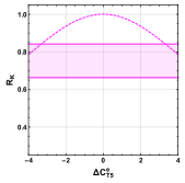
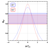
Figure 1: Variation of $R_{K}^{\rm cen}$, $R_{K^{*}}^{\rm low}$ and $R_{K^{*}}^{\rm cen}$ with $\Delta C_{T5}^{e}$. The horizontal bands correspond to the experimental $1\sigma$ upper and lower limits shown in Table-1.

It can be seen from the left panel of Fig. 1 that $\Delta C_{T5}^{e}\sim\pm 1$ not only explains $R_{K^{*}}^{\rm cen}$ and $R_{K^{*}}^{\rm low}$ simultaneously but also brings them close to the experimental central values. As pointed out by one of the authors in Ghosh:2017ber , this is not possible naturally by any other local operator at the dimension-6 level, and in this sense, the tensor operators are unique. However, as can be seen from the right panel of Fig. 1, $\Delta C_{T5}^{e}\sim\pm 1$ can not reduce $R_{K}^{\rm cen}$ much from its SM value of unity, and hence a simultaneous explanation of $R_{K}^{\rm cen}$, $R_{K^{*}}^{\rm cen}$ and $R_{K^{*}}^{\rm low}$ is not possible. All statements made here for $\Delta C_{T5}^{e}$ applies equally for the other tensor Wilson coefficient $\Delta C_{T}^{e}$.

Note that, any non-zero value for $\Delta C_{T}^{\mu}$ and $\Delta C_{T5}^{\mu}$ leads to values for $R_{K}$ and $R_{K^{*}}$ greater than their SM values and thus, tensor operators in the muon sector are ruled out as possible explanation of these anomalies.

In the following section, we will investigate whether a simultaneous solution is possible when other additional operators are also considered. While we consider only unprimed operators in the main text, the effect of the primed operators in conjunction with the tensor operators can be found in Appendix B.

4 Combination of Vector and Tensor operators

In Fig. 2, we show the regions in $\Delta C_{9}^{e}$ - $\Delta C_{T5}^{e}$ plane allowed by the experimental measurements of the various observables listed in Table-1. In the left panel, the blue, red and yellow shaded regions correspond to the $1\sigma$ experimental ranges of $R_{K^{*}}^{\rm low}$, $R_{K^{*}}^{\rm cen}$ and $R_{K}^{\rm cen}$ respectively. The black shaded regions are the overlap of the three. It should be noticed that the black shaded region is outside the $\Delta C_{T5}^{e}=0$ line, and hence no simultaneous solutions are possible with only $\Delta C_{9}^{e}$. In the right panel, we also show the regions allowed by $\mathcal{B}^{\text{low}}_{X_{s}ee}$(in blue) and $\mathcal{B}^{\text{high}}_{X_{s}ee}$ (in red). The black shaded region from the left panel is also superimposed there. It can be seen that there is a small overlap of the black, blue and red regions in the right panel where all the constraints including those from the inclusive decay are satisfied.

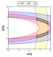
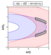
Figure 2: Allowed regions in $\Delta C_{9}^{e}$ - $\Delta C_{T5}^{e}$ plane. See text for more details.

In Fig. 3, we show the allowed regions in the $\Delta C_{9}^{\mu}$ - $\Delta C_{T5}^{e}$ plane. The various shaded regions in the left panel have the same meaning as in Fig. 2. The grey vertical (horizontal) band corresponds to the experimental $1\sigma$ allowed region of $\mathcal{B}^{\text{low}}_{X_{s}\mu\mu}$ ($\mathcal{B}^{\text{low}}_{X_{s}ee}$). Similar to the previous case, here also a simultaneous solution is not possible with only $\Delta C_{9}^{\mu}$, and non-zero tensor contribution is required. However, as can be seen from the right panel of Fig. 3, this scenario is in tension with the measurements of $\mathcal{B}^{\text{high}}_{X_{s}\ell\ell}$.

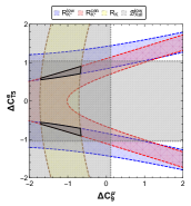
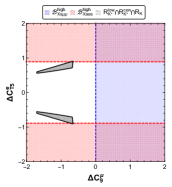
Figure 3: Allowed regions in $\Delta C_{9}^{\mu}$ - $\Delta C_{T5}^{e}$ plane. See text for more details.

We now consider the two cases $\Delta C_{9}^{e}=-\Delta C_{10}^{e}$ vs. $\Delta C_{T5}^{e}$ and $\Delta C_{9}^{\mu}=-\Delta C_{10}^{\mu}$ vs. $\Delta C_{T5}^{e}$. In Fig. 4 we show our results. It can be seen from the upper panel that $\Delta C_{9}^{\mu}=-\Delta C_{10}^{\mu}$ alone (i.e., with $\Delta C_{T5}^{e}=0$) can not explain $R_{K^{*}}^{\rm low}$, $R_{K^{*}}^{\rm cen}$ and $R_{K}^{\rm cen}$ simultaneously within their experimental $1\sigma$ regions. However, a simultaneous solutions is possible if a non-zero $\Delta C_{T5}^{e}\sim\pm 0.6$ is considered. Note that, the Wilson coefficient $C_{10}^{\mu}$ also modifies $\mathcal{B}_{\mu\mu}$ which gives a bound $0\lesssim\Delta C_{10}^{\mu}\lesssim 0.7$ at the $1\sigma$ level Ghosh:2017ber . Hence, the black overlap region in the upper left panel is allowed by $\mathcal{B}_{\mu\mu}$. However, as in Fig. 3, this scenario also is in tension with the measurements of $\mathcal{B}^{\text{high}}_{X_{s}\ell\ell}$.

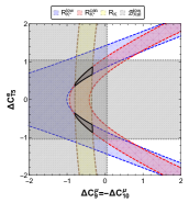
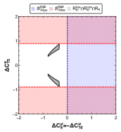
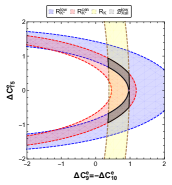
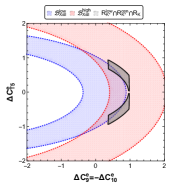
Figure 4: Allowed regions in $\Delta C_{9}^{\mu}(=-\Delta C_{10}^{\mu})$ - $\Delta C_{T5}^{e}$ plane (upper panel) and $\Delta C_{9}^{e}(=-\Delta C_{10}^{e})$ - $\Delta C_{T5}^{e}$ plane (lower panel). See text for more details.

The situation is better for $\Delta C_{9}^{e}=-\Delta C_{10}^{e}$ vs. $\Delta C_{T5}^{e}$ as shown in the bottom panel of Fig. 4. Here, a simultaneous solutions to not only $R_{K^{*}}^{\rm low}$, $R_{K^{*}}^{\rm cen}$ and $R_{K}^{\rm cen}$, but also the inclusive decay ${\bar{B}}_{d}\to X_{s}e^{+}e^{-}$ is possible. This corresponds to the small overlap of the black, red and blue shaded regions in the lower right panel of Fig. 4.

Before closing this section, we would like to mention that the tensor operators do not get generated at the dimension-6 level if $\rm SU(2)\times\rm U(1)_{Y}$ gauge invariance is imposed, which was also pointed out in Alonso:2014csa . However, it can be generated at the dimension-8 level. For example, one can write down the operator $(1/\Lambda^{4})(\overline{s_{R}}L_{1}\tilde{H})\,(\overline{\mu_{R}}Q_{3}\tilde{H})$ which, after electroweak symmetry breaking, generates the operator $(v^{2}/2\Lambda^{4})(\bar{s}P_{L}\mu)\,(\bar{\mu}P_{L}b)$. This operator can be Fierz transformed into $(v^{2}/2\Lambda^{4})(\bar{s}P_{L}b)\,(\bar{\mu}P_{L}\mu)$ and the tensor operator $(v^{2}/8\Lambda^{4})(\bar{s}\sigma_{\mu\nu}P_{L}b)\,(\bar{\mu}\sigma^{\mu\nu}P_{L}\mu)$. For more details, see Appendix C.

5 Summary

Motivated by the recent measurements of $R_{K^{*}}$ in two $q^{2}$ bins by the LHCb collaboration, we have performed a detailed analysis of the role of tensor operators in $R_{K}$ and $R_{K^{*}}$, for the first time in the literature. We show that, unlike the vector, axial vector, scalar or pseudo scalar operators, tensor operators can comfortably explain $R_{K^{*}}^{\rm cen}$ and $R_{K^{*}}^{\rm low}$ simultaneously. Hence, if the experimental measurement of $R_{K^{*}}$ in the low $q^{2}$ bin stays in the future, either a very light vector boson (as shown by one of the authors in Ghosh:2014awa ) or the existence of tensor operators would be unavoidable. However, we find that a simultaneous explanation of $R_{K}$ also would require the existence of other Wilson coefficients (of vector and/or axial vector operators, for example) in conjunction with the tensor operators. We study the interplay of the vector and axial vector operators with the tensor structures, and obtain the regions allowed by the $1\sigma$ experimental values of $R_{K}$ and $R_{K^{*}}$. We further show that the measured branching ratios for the inclusive $B_{d}\to X_{s}\ell^{+}\ell^{-}$ decay provide very important constraints on the various solutions. We also present completely general numerical formulae which can be used to effortlessly compute $R_{K}^{\rm cen}$, $R_{K^{*}}^{\rm cen}$, $R_{K^{*}}^{\rm low}$ and the inclusive branching fractions just knowing the short distance Wilson coefficients at the $m_{b}$ scale.

——————————————————————————–

Appendix A Complete expressions for the branching ratios

$$\dfrac{{\cal B}_{Kee}^{\rm cen}}{{\cal B}_{Kee}^{\rm cen}|_{\rm SM}}=1 +0.2429[\Delta C_{9}^{e}]+0.0274[\Delta C_{9}^{e}]^{2}+0.2429[\Delta C_{9^{\prime}}^{e}]+0.0549[\Delta C_{9}^{e}][\Delta C_{9^{\prime}}^{e}]+0.0274[\Delta C_{9^{\prime}}^{e}]^{2}-0.225[\Delta C_{10}^{e}]$$ (6)

$$+0.0274[\Delta C_{10}^{e}]^{2}-0.225[\Delta C_{10^{\prime}}^{e}]+0.0549[\Delta C_{10}^{e}][\Delta C_{10^{\prime}}^{e}]+0.0274[\Delta C_{10^{\prime}}^{e}]^{2}+0.0092[\Delta C_{S}^{e}]^{2}$$

$$+0.0184[\Delta C_{S}^{e}][\Delta C_{S^{\prime}}^{e}]+0.0092[\Delta C_{S^{\prime}}^{e}]^{2}+0.0092[\Delta C_{P}^{e}]^{2}+0.0184[\Delta C_{P}^{e}][\Delta C_{P^{\prime}}^{e}]+0.0092[\Delta C_{P^{\prime}}^{e}]^{2}$$

$$+0.0002[\Delta C_{T}^{e}]+0.0171[\Delta C_{T}^{e}]^{2}+0.0171[\Delta C_{T5}^{e}]^{2}$$

$$\dfrac{{\cal B}_{K\mu\mu}^{\rm cen}}{{\cal B}_{K\mu\mu}^{\rm cen}|_{\rm SM}}=1 +0.2427[\Delta C_{9}^{\mu}]+0.0274[\Delta C_{9}^{\mu}]^{2}+0.2427[\Delta C_{9^{\prime}}^{\mu}]+0.0548[\Delta C_{9}^{\mu}][\Delta C_{9^{\prime}}^{\mu}]+0.0274[\Delta C_{9^{\prime}}^{\mu}]^{2}-0.2253[\Delta C_{10}^{\mu}]$$ (7)

$$+0.0275[\Delta C_{10}^{\mu}]^{2}-0.225[\Delta C_{10^{\prime}}^{\mu}]+0.055[\Delta C_{10}^{\mu}][\Delta C_{10^{\prime}}^{\mu}]+0.0275[\Delta C_{10^{\prime}}^{\mu}]^{2}+0.009[\Delta C_{S}^{\mu}]^{2}$$

$$+0.018[\Delta C_{S}^{\mu}][\Delta C_{S^{\prime}}^{\mu}]+0.009[\Delta C_{S^{\prime}}^{\mu}]^{2}-0.0187[\Delta C_{P}^{\mu}]+0.0046\big{(}[\Delta C_{10}^{\mu}]+[\Delta C_{10^{\prime}}^{\mu}]\big{)}\big{(}[\Delta C_{P}^{\mu}]+[\Delta C_{P^{\prime}}^{\mu}]\big{)}$$

$$+0.0091[\Delta C_{P}^{\mu}]^{2}-0.0187[\Delta C_{P^{\prime}}^{\mu}]+0.0182[\Delta C_{P}^{\mu}][\Delta C_{P^{\prime}}^{\mu}]+0.0091[\Delta C_{P^{\prime}}^{\mu}]^{2}+0.0168[\Delta C_{T5}^{\mu}]^{2}$$

$$+0.0457[\Delta C_{T}^{\mu}]+0.0103\big{(}[\Delta C_{9}^{\mu}]+[\Delta C_{9^{\prime}}^{\mu}]\big{)}[\Delta C_{T}^{\mu}]+0.0174[\Delta C_{T}^{\mu}]^{2}$$

$$\dfrac{{\cal B}_{K^{*}ee}^{\rm low}}{{\cal B}_{K^{*}ee}^{\rm low}|_{\rm SM}}=1 +0.0764[\Delta C_{9}^{e}]+0.0136[\Delta C_{9}^{e}]^{2}-0.1048[\Delta C_{9^{\prime}}^{e}]-0.0257[\Delta C_{9}^{e}][\Delta C_{9^{\prime}}^{e}]+0.0136[\Delta C_{9^{\prime}}^{e}]^{2}-0.1118[\Delta C_{10}^{e}]$$ (8)

$$+0.0136[\Delta C_{10}^{e}]^{2}+0.1054[\Delta C_{10^{\prime}}^{e}]-0.0257[\Delta C_{10}^{e}][\Delta C_{10^{\prime}}^{e}]+0.0136[\Delta C_{10^{\prime}}^{e}]^{2}+0.0006\big{(}[\Delta C_{S}^{e}]-[\Delta C_{S^{\prime}}^{e}]\big{)}^{2}$$

$$+0.0006\big{(}[\Delta C_{P}^{e}]-[\Delta C_{P^{\prime}}^{e}]\big{)}^{2}-0.0015[\Delta C_{T}^{e}]+0.2901[\Delta C_{T}^{e}]^{2}-0.0013[\Delta C_{T5}^{e}]+0.2901[\Delta C_{T5}^{e}]^{2}$$

$$\dfrac{{\cal B}_{K^{*}\mu\mu}^{\rm low}}{{\cal B}_{K^{*}\mu\mu}^{\rm low}|_{\rm SM}}=1 +0.0806[\Delta C_{9}^{\mu}]+0.0144[\Delta C_{9}^{\mu}]^{2}-0.1103[\Delta C_{9^{\prime}}^{\mu}]-0.027[\Delta C_{9}^{\mu}][\Delta C_{9^{\prime}}^{\mu}]+0.0144[\Delta C_{9^{\prime}}^{\mu}]^{2}-0.1167[\Delta C_{10}^{\mu}]$$ (9)

$$+0.0142[\Delta C_{10}^{\mu}]^{2}+0.1106[\Delta C_{10^{\prime}}^{\mu}]-0.027[\Delta C_{10}^{\mu}][\Delta C_{10^{\prime}}^{\mu}]+0.0142[\Delta C_{10^{\prime}}^{\mu}]^{2}+0.0006[\Delta C_{S}^{\mu}]^{2}$$

$$-0.0012[\Delta C_{S}^{\mu}][\Delta C_{S^{\prime}}^{\mu}]+0.0006[\Delta C_{S^{\prime}}^{\mu}]^{2}-0.0078[\Delta C_{P}^{\mu}]+0.0019[\Delta C_{10}^{\mu}][\Delta C_{P}^{\mu}]-0.0019[\Delta C_{10^{\prime}}^{\mu}][\Delta C_{P}^{\mu}]$$

$$+0.0006[\Delta C_{P}^{\mu}]^{2}+0.0078[\Delta C_{P^{\prime}}^{\mu}]-0.0019[\Delta C_{10}^{\mu}][\Delta C_{P^{\prime}}^{\mu}]+0.0019[\Delta C_{10^{\prime}}^{\mu}][\Delta C_{P^{\prime}}^{\mu}]-0.0013[\Delta C_{P}^{\mu}][\Delta C_{P^{\prime}}^{\mu}]$$

$$+0.0006[\Delta C_{P^{\prime}}^{\mu}]^{2}-0.2362[\Delta C_{T5}^{\mu}]+0.0165[\Delta C_{9}^{\mu}][\Delta C_{T5}^{\mu}]-0.0165[\Delta C_{9^{\prime}}^{\mu}][\Delta C_{T5}^{\mu}]+0.3057[\Delta C_{T5}^{\mu}]^{2}$$

$$-0.2676[\Delta C_{T}^{\mu}]+0.0088[\Delta C_{9}^{\mu}][\Delta C_{T}^{\mu}]+0.0088[\Delta C_{9^{\prime}}^{\mu}][\Delta C_{T}^{\mu}]+0.305[\Delta C_{T}^{\mu}]^{2}$$

$$\dfrac{{\cal B}_{K^{*}ee}^{\rm cen}}{{\cal B}_{K^{*}ee}^{\rm cen}|_{\rm SM}}=1 +0.2187[\Delta C_{9}^{e}]+0.032[\Delta C_{9}^{e}]^{2}-0.1998[\Delta C_{9^{\prime}}^{e}]-0.0474[\Delta C_{9}^{e}][\Delta C_{9^{\prime}}^{e}]+0.032[\Delta C_{9^{\prime}}^{e}]^{2}-0.2629[\Delta C_{10}^{e}]$$ (10)

$$+0.032[\Delta C_{10}^{e}]^{2}+0.1945[\Delta C_{10^{\prime}}^{e}]-0.0474[\Delta C_{10}^{e}][\Delta C_{10^{\prime}}^{e}]+0.032[\Delta C_{10^{\prime}}^{e}]^{2}+0.0067[\Delta C_{S}^{e}]^{2}$$

$$-0.0134[\Delta C_{S}^{e}][\Delta C_{S^{\prime}}^{e}]+0.0067[\Delta C_{S^{\prime}}^{e}]^{2}+0.0067[\Delta C_{P}^{e}]^{2}-0.0134[\Delta C_{P}^{e}][\Delta C_{P^{\prime}}^{e}]+0.0067[\Delta C_{P^{\prime}}^{e}]^{2}$$

$$+0.5349[\Delta C_{T}^{e}]^{2}+0.0003[\Delta C_{T5}^{e}]+0.0001[\Delta C_{9}^{e}][\Delta C_{T5}^{e}]-0.0001[\Delta C_{9^{\prime}}^{e}][\Delta C_{T5}^{e}]+0.5349[\Delta C_{T5}^{e}]^{2}$$

$$\dfrac{{\cal B}_{K^{*}\mu\mu}^{\rm cen}}{{\cal B}_{K^{*}\mu\mu}^{\rm cen}|_{\rm SM}}=1 +0.2194[\Delta C_{9}^{\mu}]+0.0321[\Delta C_{9}^{\mu}]^{2}-0.2004[\Delta C_{9^{\prime}}^{\mu}]-0.0476[\Delta C_{9}^{\mu}][\Delta C_{9^{\prime}}^{\mu}]+0.0321[\Delta C_{9^{\prime}}^{\mu}]^{2}-0.2622[\Delta C_{10}^{\mu}]$$ (11)

$$+0.032[\Delta C_{10}^{\mu}]^{2}+0.1949[\Delta C_{10^{\prime}}^{\mu}]-0.0475[\Delta C_{10}^{\mu}][\Delta C_{10^{\prime}}^{\mu}]+0.032[\Delta C_{10^{\prime}}^{\mu}]^{2}+0.0066[\Delta C_{S}^{\mu}]^{2}$$

$$-0.0132[\Delta C_{S}^{\mu}][\Delta C_{S^{\prime}}^{\mu}]+0.0066[\Delta C_{S^{\prime}}^{\mu}]^{2}-0.0138[\Delta C_{P}^{\mu}]+0.0034[\Delta C_{10}^{\mu}][\Delta C_{P}^{\mu}]-0.0034[\Delta C_{10^{\prime}}^{\mu}][\Delta C_{P}^{\mu}]$$

$$+0.0067[\Delta C_{P}^{\mu}]^{2}+0.0138[\Delta C_{P^{\prime}}^{\mu}]-0.0034[\Delta C_{10}^{\mu}][\Delta C_{P^{\prime}}^{\mu}]+0.0034[\Delta C_{10^{\prime}}^{\mu}][\Delta C_{P^{\prime}}^{\mu}]-0.0134[\Delta C_{P}^{\mu}][\Delta C_{P^{\prime}}^{\mu}]$$

$$+0.0067[\Delta C_{P^{\prime}}^{\mu}]^{2}+0.0638[\Delta C_{T5}^{\mu}]+0.0295[\Delta C_{9}^{\mu}][\Delta C_{T5}^{\mu}]-0.0295[\Delta C_{9^{\prime}}^{\mu}][\Delta C_{T5}^{\mu}]+0.5373[\Delta C_{T5}^{\mu}]^{2}$$

$$+0.0039[\Delta C_{T}^{\mu}]+0.0154[\Delta C_{9}^{\mu}][\Delta C_{T}^{\mu}]+0.0154[\Delta C_{9^{\prime}}^{\mu}][\Delta C_{T}^{\mu}]+0.5359[\Delta C_{T}^{\mu}]^{2}$$

$$10^{6}{\cal B}_{X_{s}\ell\ell}^{\rm low}= 10^{6}{\cal B}_{X_{s}\ell\ell}^{\rm low}|_{\rm SM}+0.4156[\Delta C_{9}^{\ell}]+0.0647\big{(}[\Delta C_{9}^{\ell}]^{2}+[\Delta C_{9^{\prime}}^{\ell}]^{2}+[\Delta C_{10}^{\ell}]^{2}+[\Delta C_{10^{\prime}}^{\ell}]^{2}\big{)}-0.5308[\Delta C_{10}^{\ell}]$$ (12)

$$+0.0108\big{(}[\Delta C_{S}^{\ell}]^{2}+[\Delta C_{S^{\prime}}^{\ell}]^{2}+[\Delta C_{P}^{\ell}]^{2}+[\Delta C_{P^{\prime}}^{\ell}]^{2}\big{)}+0.8615\big{(}[\Delta C_{T5}^{\ell}]^{2}+[\Delta C_{T}^{\ell}]^{2}\big{)}$$

$$10^{6}{\cal B}_{X_{s}\ell\ell}^{\rm high}= 10^{6}{\cal B}_{X_{s}\ell\ell}^{\rm high}|_{\rm SM}+0.1187[\Delta C_{9}^{\ell}]+0.0143\big{(}[\Delta C_{9}^{\ell}]^{2}+[\Delta C_{9^{\prime}}^{\ell}]^{2}+[\Delta C_{10}^{\ell}]^{2}\big{)}-0.1171[\Delta C_{10}^{\ell}]+0.0143[\Delta C_{10^{\prime}}^{\ell}]^{2}$$ (13)

$$+0.0063\big{(}[\Delta C_{S}^{\ell}]^{2}+[\Delta C_{S^{\prime}}^{\ell}]^{2}+[\Delta C_{P}^{\ell}]^{2}+[\Delta C_{P^{\prime}}^{\ell}]^{2}\big{)}+0.1272\big{(}[\Delta C_{T5}^{\ell}]^{2}+[\Delta C_{T}^{\ell}]^{2}\big{)}$$

Appendix B Primed operators

Earlier we considered only the unprimed vector and axial vector operators namely, $C_{9}^{\mu,e}$ and $C_{10}^{\mu,e}$, and neglected their primed counterparts $C_{9^{\prime}}^{\mu,e}$ and $C_{10^{\prime}}^{\mu,e}$. It has been shown (see for example, Ghosh:2014awa ) that the primed operators alone are unable to produce the experimental measurements of $R_{K}$ and $R_{K^{*}}$ simultaneously. In this section, we will investigate whether the situation can improve in the presence of tensor operators.

Fig. 5 shows the allowed regions in $\Delta C_{9^{\prime}}^{\mu}$ - $\Delta C_{T5}^{e}$ plane.

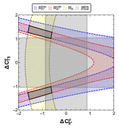
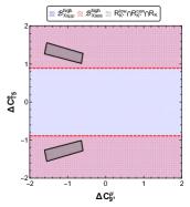
Figure 5: Allowed regions in $\Delta C_{9^{\prime}}^{\mu}$ - $\Delta C_{T5}^{e}$ plane. See text for more details.

It can be seen that in order to satisfy $R_{K}^{\rm cen}$, $R_{K^{\ast}}^{\rm low}$ and $R_{K^{\ast}}^{\rm cen}$ simultaneously in the presence of $\Delta C_{9^{\prime}}^{\mu}$, large value of $\Delta C_{T5}^{e}\approx\pm 1.3$ is also needed.

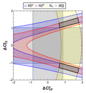
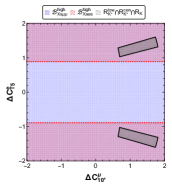
Figure 6: Allowed regions in $\Delta C_{10^{\prime}}^{\mu}$ - $\Delta C_{T5}^{e}$ plane. See text for more details.

However, this solution is in tension with $\mathcal{B}^{\text{low}}_{X_{s}ee}$ as can be seen from the grey region in the left panel of Fig. 5. Note that, in the right panel of Fig. 5 the blue region covers the whole plane, and hence this solution is consistent with $\mathcal{B}^{\text{high}}_{X_{s}\ell\ell}$. Similar statements can be made also for $\Delta C_{10^{\prime}}^{\mu}$, as can be seen from Fig. 6.

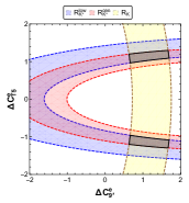
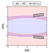
Figure 7: Allowed regions in $\Delta C_{9^{\prime}}^{e}$ - $\Delta C_{T5}^{e}$ plane. See text for more details.

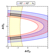
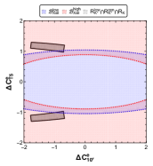
Figure 8: Allowed regions in $\Delta C_{10^{\prime}}^{e}$ - $\Delta C_{T5}^{e}$ plane. See text for more details.

Fig. 7 and Fig. 8 show the allowed regions in $\Delta C_{9^{\prime}}^{e}$ vs. $\Delta C_{T5}^{e}$ and $\Delta C_{10^{\prime}}^{e}$ vs. $\Delta C_{T5}^{e}$ planes respectively. In these cases also, the primed operators can be allowed if a large tensor contribution exists at the same time.

Appendix C SU(2) $\times$ U(1)_Y gauge invariance

As mentioned in the main text, the tensor operators do not get generated at the dimension-6 level if SU(2) $\times$ U(1)_Y gauge invariance is imposed. However, they can be generated at the dimension-8 level. Here we show a few examples,

$$1.~{}~{} \frac{C_{Y_{d}Y_{\ell}}}{\Lambda^{4}}[\overline{s_{R}}\sigma^{\mu\nu}Q_{3}\tilde{H}][\overline{e_{\ell R}}\sigma_{\mu\nu}L_{\ell}\tilde{H}]$$ (14)

$$\to\frac{1}{2}C_{Y_{d}Y_{\ell}}\frac{v^{2}}{\Lambda^{4}}[\overline{s_{R}}\sigma^{\mu\nu}b_{L}][\overline{e_{\ell R}}\sigma_{\mu\nu}e_{\ell L}]$$

$$=\frac{1}{4}C_{Y_{d}Y_{\ell}}\frac{v^{2}}{\Lambda^{4}}\left({\cal O}_{T}-{\cal O}_{T5}\right)$$

$$2.~{}~{} \frac{C_{sLeQ}}{\Lambda^{4}}[\overline{s_{R}}L_{\ell}\tilde{H}][\overline{e_{\ell R}}Q_{3}\tilde{H}]$$ (15)

$$\to\frac{C_{sLeQ}}{\Lambda^{4}}\bigg{(}\frac{1}{2}[\overline{s_{R}}Q_{3}\tilde{H}][\overline{e_{\ell R}}L_{\ell}\tilde{H}]$$

$$\hskip 56.9055pt+\frac{1}{8}[\overline{s_{R}}\sigma^{\mu\nu}Q_{3}\tilde{H}][\overline{e_{\ell R}}\sigma_{\mu\nu}L_{\ell}\tilde{H}]\bigg{)}$$

$$=\frac{1}{8}C_{sLeQ}\frac{v^{2}}{\Lambda^{4}}\left({\cal O}_{S^{\prime}}-{\cal O}_{P^{\prime}}+\frac{1}{4}{\cal O}_{T}-\frac{1}{4}{\cal O}_{T5}\right)$$

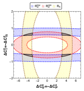
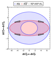
Figure 9: Allowed regions in $\Delta C_{S^{\prime}}^{e}(=-\Delta C_{P^{\prime}}^{e})$ vs. $\Delta C_{T5}^{e}(=-\Delta C_{T}^{e})$ plane. See text for more details.

It is hard to generate only the tensor operators in a complete field theory model. The second operator above is much easier to generate (it can be generated even at the tree level). In this case, however, both scalar and tensor operators are generated with the following relations among the Wilson coefficients,

$$\Delta C_{S^{\prime}}^{e}=-\Delta C_{P^{\prime}}^{e}=4\Delta C_{T5}^{e}=-4\Delta C_{T}^{e}\,.$$ (16)

Note that, gauge invariance at the dimension 6 level always leads to the relation $\Delta C_{S^{\prime}}^{e}=+\Delta C_{P^{\prime}}^{e}$ Alonso:2014csa , which is now broken by the dimension 8 operators. In Fig. 9, we show the various allowed regions in the $\Delta C_{S^{\prime}}^{e}(=-\Delta C_{P^{\prime}}^{e})$ vs. $\Delta C_{T5}^{e}(=-\Delta C_{T}^{e})$ plane. It is interesting that the black overlap regions in the left panel satisfy Eq. (16) approximately. In fact, there is tiny region in the right panel which satisfies the inclusive measurements too.

Note that, the value of $\Delta C_{S^{\prime}}^{e}=-\Delta C_{P^{\prime}}^{e}\approx 3$ corresponds to a NP scale $\Lambda\sim(C_{sLeQ})^{1/4}\,1.5~{}\rm TeV$. While the scale is rather low, it is still intriguing that one local operator in Eq. (15) can explain all the anomalies (including $R_{K^{*}}^{\rm low}$) simultaneously. Unfortunately, for such large value $\Delta C_{S^{\prime}}^{e}=-\Delta C_{P^{\prime}}^{e}\approx 3$, $\mathcal{B}_{ee}$ exceeds the experimental upper bound, and some cancellation, either from other dimension-8 operators or from dimension-6 operators would be necessary for this operator to be viable. More detailed exploration of such dynamics is left for future work.

——————————————————————————–

References

- (1) LHCb, R. Aaij et al., (2017), 1705.05802.
- (2) LHCb collaboration, R. Aaij et al., (2014), 1406.6482.
- (3) G. Hiller and F. Kruger, Phys. Rev. D69 (2004) 074020, hep-ph/0310219.
- (4) M. Bordone, G. Isidori and A. Pattori, Eur. Phys. J. C76 (2016) 440, 1605.07633.
- (5) W. Altmannshofer et al., JHEP 0901 (2009) 019, 0811.1214.
- (6) A.K. Alok et al., JHEP 1002 (2010) 053, 0912.1382.
- (7) A.K. Alok et al., JHEP 1111 (2011) 121, 1008.2367.
- (8) A.K. Alok et al., JHEP 1111 (2011) 122, 1103.5344.
- (9) S. Descotes-Genon et al., JHEP 1106 (2011) 099, 1104.3342.
- (10) W. Altmannshofer, P. Paradisi and D.M. Straub, JHEP 1204 (2012) 008, 1111.1257.
- (11) J. Matias et al., JHEP 1204 (2012) 104, 1202.4266.
- (12) S. Descotes-Genon et al., JHEP 1301 (2013) 048, 1207.2753.
- (13) J. Lyon and R. Zwicky, (2013), 1305.4797.
- (14) S. Descotes-Genon, J. Matias and J. Virto, Phys.Rev. D88 (2013) 074002, 1307.5683.
- (15) W. Altmannshofer and D.M. Straub, Eur.Phys.J. C73 (2013) 2646, 1308.1501.
- (16) A.J. Buras and J. Girrbach, JHEP 1312 (2013) 009, 1309.2466.
- (17) A. Datta, M. Duraisamy and D. Ghosh, Phys.Rev. D89 (2014) 071501, 1310.1937.
- (18) W. Altmannshofer et al., Phys.Rev. D89 (2014) 095033, 1403.1269.
- (19) R. Alonso, B. Grinstein and J. Martin Camalich, Phys. Rev. Lett. 113 (2014) 241802, 1407.7044.
- (20) D. Ghosh, M. Nardecchia and S.A. Renner, JHEP 12 (2014) 131, 1408.4097.
- (21) F.S. Queiroz, K. Sinha and A. Strumia, Phys. Rev. D91 (2015) 035006, 1409.6301.
- (22) R. Mandal, R. Sinha and D. Das, Phys. Rev. D90 (2014) 096006, 1409.3088.
- (23) B. Gripaios, M. Nardecchia and S.A. Renner, JHEP 05 (2015) 006, 1412.1791.
- (24) A. Greljo, G. Isidori and D. Marzocca, JHEP 07 (2015) 142, 1506.01705.
- (25) B. Gripaios, M. Nardecchia and S.A. Renner, JHEP 06 (2016) 083, 1509.05020.
- (26) R. Alonso, B. Grinstein and J. Martin Camalich, JHEP 10 (2015) 184, 1505.05164.
- (27) R. Barbieri et al., Eur. Phys. J. C76 (2016) 67, 1512.01560.
- (28) A. Falkowski, M. Nardecchia and R. Ziegler, JHEP 11 (2015) 173, 1509.01249.
- (29) A. Crivellin, G. D’Ambrosio and J. Heeck, Phys. Rev. D91 (2015) 075006, 1503.03477.
- (30) A. Crivellin et al., Phys. Rev. D92 (2015) 054013, 1504.07928.
- (31) G. Belanger, C. Delaunay and S. Westhoff, Phys. Rev. D92 (2015) 055021, 1507.06660.
- (32) A. Carmona and F. Goertz, Phys. Rev. Lett. 116 (2016) 251801, 1510.07658.
- (33) R. Mandal and R. Sinha, Phys. Rev. D95 (2017) 014026, 1506.04535.
- (34) S. Sahoo and R. Mohanta, Phys. Rev. D91 (2015) 094019, 1501.05193.
- (35) S. Sahoo, R. Mohanta and A.K. Giri, Phys. Rev. D95 (2017) 035027, 1609.04367.
- (36) A. Crivellin et al., Phys. Lett. B766 (2017) 77, 1611.02703.
- (37) F. Feruglio, P. Paradisi and A. Pattori, Phys. Rev. Lett. 118 (2017) 011801, 1606.00524.
- (38) R. Barbieri, C.W. Murphy and F. Senia, Eur. Phys. J. C77 (2017) 8, 1611.04930.
- (39) I. Garcia Garcia, JHEP 03 (2017) 040, 1611.03507.
- (40) E. Megias et al., JHEP 09 (2016) 118, 1608.02362.
- (41) B. Bhattacharya et al., JHEP 01 (2017) 015, 1609.09078.
- (42) D. Bhatia, S. Chakraborty and A. Dighe, JHEP 03 (2017) 117, 1701.05825.
- (43) E. Megias, M. Quiros and L. Salas, (2017), 1703.06019.
- (44) A. Datta, J. Liao and D. Marfatia, Phys. Lett. B768 (2017) 265, 1702.01099.
- (45) M. Bordone, G. Isidori and S. Trifinopoulos, (2017), 1702.07238.
- (46) S. Di Chiara et al., (2017), 1704.06200.
- (47) B. Capdevila et al., (2017), 1704.05340.
- (48) W. Altmannshofer, P. Stangl and D.M. Straub, (2017), 1704.05435.
- (49) G. D’Amico et al., (2017), 1704.05438.
- (50) G. Hiller and I. Nisandzic, (2017), 1704.05444.
- (51) L.S. Geng et al., (2017), 1704.05446.
- (52) M. Ciuchini et al., (2017), 1704.05447.
- (53) A. Celis et al., (2017), 1704.05672.
- (54) D. Becirevic and O. Sumensari, (2017), 1704.05835.
- (55) D. Ghosh, (2017), 1704.06240.
- (56) A.K. Alok et al., (2017), 1704.07347.
- (57) A.K. Alok et al., (2017), 1704.07397.
- (58) W. Wang and S. Zhao, (2017), 1704.08168.
- (59) F. Feruglio, P. Paradisi and A. Pattori, (2017), 1705.00929.
- (60) J. Ellis, M. Fairbairn and P. Tunney, (2017), 1705.03447.
- (61) R. Alonso et al., (2017), 1704.08158.
- (62) F. Bishara, U. Haisch and P.F. Monni, (2017), 1705.03465.
- (63) R. Alonso et al., (2017), 1705.03858.
- (64) Y. Tang and Y.L. Wu, (2017), 1705.05643.
- (65) A. Datta et al., (2017), 1705.08423.
- (66) D. Das et al., (2017), 1705.09188.
- (67) C. Bobeth, G. Hiller and D. van Dyk, Phys.Rev. D87 (2013) 034016, 1212.2321.
- (68) J. Gratrex, M. Hopfer and R. Zwicky, Phys. Rev. D93 (2016) 054008, 1506.03970.
- (69) S. Descotes-Genon et al., JHEP 06 (2016) 092, 1510.04239.
- (70) C. Bobeth et al., Phys.Rev.Lett. 112 (2014) 101801, 1311.0903.
- (71) R. Fleischer, R. Jaarsma and G. Tetlalmatzi-Xolocotzi, (2017), 1703.10160.
- (72) CMS, S. Chatrchyan et al., Phys. Rev. Lett. 111 (2013) 101804, 1307.5025.
- (73) LHCb, R. Aaij et al., (2017), 1703.05747.
- (74) CDF, T. Aaltonen et al., Phys. Rev. Lett. 102 (2009) 201801, 0901.3803.
- (75) T. Huber, T. Hurth and E. Lunghi, Nucl.Phys. B802 (2008) 40, 0712.3009.
- (76) BaBar, J.P. Lees et al., Phys. Rev. Lett. 112 (2014) 211802, 1312.5364.
- (77) P. Ball, G.W. Jones and R. Zwicky, Phys. Rev. D75 (2007) 054004, hep-ph/0612081.
- (78) A. Khodjamirian et al., JHEP 1009 (2010) 089, 1006.4945.
- (79) M. Dimou, J. Lyon and R. Zwicky, Phys. Rev. D87 (2013) 074008, 1212.2242.
- (80) S. Jager and J. Martin Camalich, JHEP 05 (2013) 043, 1212.2263.
- (81) J. Lyon and R. Zwicky, (2014), 1406.0566.
- (82) M. Ciuchini et al., JHEP 06 (2016) 116, 1512.07157.
- (83) S. Jager and J. Martin Camalich, Phys. Rev. D93 (2016) 014028, 1412.3183.
- (84) B. Capdevila et al., JHEP 04 (2017) 016, 1701.08672.
- (85) Belle, S. Wehle et al., Phys. Rev. Lett. 118 (2017) 111801, 1612.05014.
- (86) HPQCD, C. Bouchard et al., Phys. Rev. D88 (2013) 054509, 1306.2384, [Erratum: Phys. Rev.D88,no.7,079901(2013)].
- (87) A. Bharucha, D.M. Straub and R. Zwicky, JHEP 08 (2016) 098, 1503.05534.
- (88) G. Hiller and M. Schmaltz, Phys. Rev. D90 (2014) 054014, 1408.1627.
- (89) P. Biancofiore, P. Colangelo and F. De Fazio, Phys. Rev. D87 (2013) 074010, 1302.1042.
- (90) D. Bardhan, P. Byakti and D. Ghosh, JHEP 01 (2017) 125, 1610.03038.