Synthesizing Mapping Relationships Using Table Corpus

Abstract

Mapping relationships, such as (country, country-code) or (company, stock-ticker), are versatile data assets for an array of applications in data cleaning and data integration like auto-correction and auto-join. However, today there are no good repositories of mapping tables that can enable these intelligent applications.

Given a corpus of tables such as web tables or spreadsheet tables, we observe that values of these mappings often exist in pairs of columns in same tables. Motivated by their broad applicability, we study the problem of synthesizing mapping relationships using a large table corpus. Our synthesis process leverages compatibility of tables based on co-occurrence statistics, as well as constraints such as functional dependency. Experiment results using web tables and enterprise spreadsheets suggest that the proposed approach can produce high quality mappings.

1 Introduction

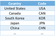
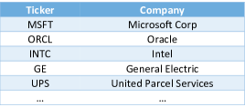
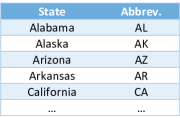
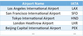
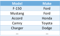
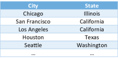
Mapping tables, sometimes also referred to as bridge tables [27], are two-column tables where each distinct value in the left column maps to a unique value in the right column (or functional dependencies hold). Table 1 gives a few example mapping tables with one-to-one mapping relationships. Table 2 shows additional examples with many-to-one mappings.

(a) ISO country codes

(b) Stock tickers

(c) State abbreviations

(d) Airport IATA codes

Table 1: Example one-to-one mapping tables: (a) Countries to ISO codes, (b) Company names to stock-tickers, (c) State names to abbreviations, (d) Airports to IATA-codes.

(a) Car make and model

(b) City and state

Table 2: Example many-to-one mapping tables: (a) Car makes and models, (b) Cities and states

Table 3: Auto-correction: correct inconsistent values (highlighted) using Table 1(c).

Table 4: Auto-fill: automatically populate values based on mappings from Table 2(b).

Table 5: Auto-join: joining related tuples based on mappings from Table 1(b)

Mapping tables like these are important data assets for a variety of applications such as data integration and data cleaning. We briefly discuss three scenarios here.

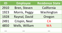
Auto-correction. Real-world tables are often dirty, where inconsistent values may be present in same columns. Table 4 shows such an example. The last column about state are mixed with both full state names and state abbreviations. An intelligent data quality agent, equipped with the mapping table in Table 1(c), can easily detect and alert users about such inconsistency, by discovering that values in the left and right column of Table 1(c) are mixed in one user data column. Furthermore, it can automatically suggest corrections based on the mapping relationship (e.g., correcting CA to California).

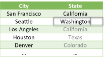
Auto-fill. In this example scenario in Table 4, a user has a list of city names. She wants to add a column of state names corresponding to the cities. By just entering a few example values (e.g., California for San Francisco), the system automatically discovers the intent by matching existing value pairs with those in Table 2(b), and can thus suggest to automatically fill remaining values in the right column (grayed out in Table 4).

Auto-join. In data integration and ad-hoc data analysis, users often need to “join” two tables together, whose key columns may have different representations. In Table 5 for example, an analyst needs to join the left table that has stocks by their market capitalization, with the right table that lists companies by their political contributions, to analyze potential correlations. However a direct join is not possible since the subject column of the left table is stock tickers, while the right table uses company names. A system equipped with mapping tables would make the join possible by using Table 1(b) as an intermediate bridge that performs a three-way join to connect these two user tables, without asking users to provide an explicit mappings.

Synthesize mapping tables with human curation. In this work, we develop methods to automatically synthesize mapping relationships from existing table corpora, where the goal is to generate as many high-quality mappings as possible. Because algorithms are bound to make mistakes, additional human verification and curation can be used to ensure very high precision (Section 4.3). The resulting mappings can then be utilized to enable the applications discussed above in a unified manner.

Why pre-compute mappings. While there are separate solutions for auto-join and auto-fill problems (e.g., [24, 38]), our approach has a few important advantages.

First, synthesized mappings are amenable to human inspection and curation, which is critical to ensure very high quality. In attempting to commercialize technologies similar to [24, 38] in enterprise spreadsheet software like Excel, the main feedback we received is the trustworthiness of results produced by black-box algorithms. Algorithms with even $99\%$ correctness is still unacceptable in the context of enterprise spreadsheets, because any error introduced by algorithms would be difficult for users to detect, but is highly embarrassing and damaging in enterprise settings.

An analogy we would like to draw is the knowledge-bases used in search engines such as Google and Microsoft Bing. Similar to our problem, the quality required for knowledge-bases is also very high, so commercial knowledge bases are created in offline processes that combine algorithmic automation with human curation. Mapping tables can be viewed as the counterpart of knowledge bases in the relational world, where a similar curation process may be needed because of the quality requirement. And like search engines that have millions of users, spreadsheet software can reach millions of data analysts, such that the cost of curating mappings can be amortized over a large user base to make the effort worthwhile.

Second, synthesized mapping relationships can be materialized as tables, which are easy to index and efficient to scale to large problems. For example, instead of performing expensive online reasoning over large table corpora for specific applications like auto-join [24] and auto-fill [38], one could index synthesized mapping tables using hash-based techniques (e.g., bloom filters) for efficiently lookup based on value containment. Such logic is both simple to implement and easy to scale.

Lastly, mapping tables are versatile data assets with many applications. By solving this common underlying problem and producing mapping tables as something that can be easily plugged into other applications, it brings benefits to a broad class of applications as opposed to requiring separate reasoning logic to be developed for different applications (e.g., [24] for auto-join and [38] for auto-fill).

Why synthesize tables. Given table corpora such as HTML tables from web or spreadsheets from enterprises, fragments of useful mapping relationships exist. For example, the country and country-ISO3-code columns in Table 1(a) are often adjacent columns in same tables on the web. As such, an alternative class of approaches is to “search” tables based on input values and then ask users to select relevant ones (e.g., Google Web Tables [1], Microsoft Power Query [2], and DataXFormer [4]). However, because desired values pairs often span across multiple tables, users frequently need to search, inspect and understand table results, before manually piecing them together from multiple tables. Our experience suggests that this process is often too cumbersome for end users.

Mappings synthesized from multiple tables, on the other hand, take away the complexity and make it easy for end users. More specifically, synthesized mappings have the following benefits.

$\bullet$ Completeness. In many cases one table only covers a small fraction of mappings in the same relationship. For example, while there exist thousands of airports, a web table like Table 1(d) often lists only a small fraction of popular airports. Stitching together tables in the same relationship provides better coverage and is clearly desirable.

$\bullet$ Synonymous mentions. Each individual table from a table corpus typically only has one mention for the same entity. For example, Table 1(a) has South Korea and KOR. In reality different tables use different but synonymous names. Table 6 shows real results synthesized from many web tables, which has different synonyms of South Korea. Similarly the right part has many synonyms for Congo. Note that a specific synonym of South Korea may not necessarily co-occur with another synonym of Congo in the same web table, and the probability of co-occurrence in conjunction with synonyms of additional countries is even lower. However, any combination of these synonyms may actually be used in user tables that may require auto-join or auto-fill. Using single tables as mappings would not provide sufficient coverage in these cases. On the other hand, if all these synonyms are synthesized together as one table like in Table 6, then any combination of these synonyms can still be covered without requiring users to perform manual synthesis from multiple tables.

$\bullet$ Spurious mappings. Certain mappings that appear to hold locally in single tables may not be meaningful. For example, a random table listing departure-airport and arrival-airport may happen to have values observe functional dependency at the instance level. However, at a conceptual level this is not a useful mapping. Such a spurious mapping, when indexed from single tables, can trigger false-positive results for applications like auto-correct and auto-join. A holistic analysis of global relationships are necessary to identify true mappings from spurious ones.

Existing approaches: Given that table synthesis is needed to assist human curation, we look at existing techniques that can be used here.

Table 6: Examples from a synthesized mapping relationship (country, country-ISO3-code) using real web tables. The left table shows examples of synonyms for the country South Korea, all of which map to the same code KOR. The right table shows similar examples for Congo.

Union tables. Ling and Halevy et al. studied the problem of stitching together web tables in the same web-domain (where tables are more homogeneous) based on meta data such as column names [30]. While the technique is not designed to synthesize relationships from a large heterogeneous corpus, it is the only work we are aware of that performs table synthesis from corpora. We will show that adapting this to a large corpus of heterogeneous tables will fail, because column names are often undescriptive [15] that leads to over-grouping and low-quality mappings. For example, in Table 1(a), the column name for countries are often just name, and the column name for country-codes may be code. As a result, grouping by column names tends to lump this table with other name-to-code mappings. Our approach reasons about compatibility of tables based on values, which are more reliable in telling the true relationships.

Schema matching. There is a long and fruitful line of research on schema matching that suggests possible mappings between table columns [31]. However, schema matching is typically used in database contexts for a small number of schemas, and produces pair-wise matches for human users to evaluate. In our problem we are given hundreds of millions of schemas as input, for which pairwise human verification is infeasible, and aggregation of pairwise decisions to a group level is necessary for human curation. Furthermore, since we are only interested in mapping relationships, which are a specific type of tables that always observe functional dependencies, we can derive additional negative incompatibility induced by FDs that is not explored by schema matching. For example, there are multiple country-to-code relationships such as (country $\rightarrow$ ISO3-country-code), (country $\rightarrow$ FIFA-country-code), (country $\rightarrow$ IOC-country-code), etc, all of which share substantial value overlap as well as similar column names. Schema matching techniques would identify them as matches and merge them incorrectly, whereas we would prevent the synthesis because of the FD-based incompatibility. Considering both positive and negative signals is critical for high-quality synthesis at a large scale.

Knowledge base. Knowledge bases (KB) such as Freebase [7] and YAGO [34] have important entity-relationships that can be viewed as synthesized (semi-automatically) from different sources. However, many mappings are missing from KB. For instance, YAGO has none of the example mappings listed in Table 1 (all of which are common mappings), while Freebase misses two (stocks and airports). Furthermore, for mappings that do exist in KB, they typically do not have synonyms like the ones in Table 6. Lastly, KB have limited coverage beyond the public web domain, such as mapping (cost-center-name $\rightarrow$ cost-center-code) that is specific to enterprises domains.

Contribution. Observing that mapping relationships are well-represented in tables, we propose to automatically synthesize mapping relationships using table corpora. We formalize this as an optimization problem that maximizes positive compatibility between tables while respecting constrains of negative compatibility imposed by functional dependencies. We show a trichotomy of complexity for the resulting optimization problem, and develop an efficient algorithm that can scale to large table corpus (e.g., 100M tables). Our evaluation using real table corpora suggests that the proposed approach can synthesize high quality mapping tables.

2 Solution Overview

In this section, we first introduce notions like mapping relationships and table corpora necessary for discussions. We then give a high-level overview of our synthesis solution.

Figure 2: Solution overview with three main steps: (1) Extract candidate two-column-tables; (2) Synthesize related tables; (3) Resolve conflicts in the same relationship.

2.1 Preliminaries

Mapping relationships. The goal of this work is to discover mapping relationships. Specifically, we focus on binary mappings involving two attributes.

Definition 1

Let $R$ be a conceptual relation with two attributes $X,Y$. The relationship is a mapping relationship, denoted by $M(X,Y)$ or $X\rightarrow Y$, if for all $x\in X$, x functionally determines one and precisely one value $y\in Y$.

Examples of mapping relationships include (country $\rightarrow$ country-code) and (company $\rightarrow$ stock-ticker) as shown in Table 1 and Table 2. There is a mapping relationship between attributes country and country-code, for instance, since value in one attribute is uniquely associated with precisely one value in the other attribute.

Note that this is closely related to functional dependency (FD), traditionally defined over one physical table. We make the distinction to define mappings as conceptual relationships that can be represented in multiple tables, but may never be fully embodied in one physical table (e.g., the synthesized mapping shown in Table 6 with both South Korea and Korea (South) would not occur in one table).

Existing FD discovery work mainly focuses on efficiency (e.g., [3]), because it is intended for interactive data exploration on ad-hoc data sets. However, in our problem the key challenge is to produce high-quality synthesis of tables to assist human curation, where efficiency is not as important because the corpus is given a priori and synthesis can be run as offline jobs.

For cases where both $X\rightarrow Y$ and $Y\rightarrow X$ are mapping relationships, we call such bi-directional relationships 1:1 mappings (examples are in Table 1). If the mapping relationship only holds in one direction, then it is an N:1 mapping (Table 2).

It is worth noting that in practice, because of name ambiguity, functional relationship in some mappings may appear to only hold approximately. For example, city $\rightarrow$ state is conceptually a mapping relationship. However, when entities are represented as strings, the functional relationship may not completely hold. For example, in the same table there may be a city called Portland in the state of Oregon, and another city Portland in the state of Maine, thus giving the appearance of violating FD. To take such name ambiguity into account, we consider relationships whose surface forms are approximate mapping relationships.

Definition 2

Let $R$ be a conceptual relation with two attributes $X,Y$. The relationship is a $\theta$-approximate mapping relationship, denoted by $M_{\theta}(X,Y)$ or $X\rightarrow_{\theta}Y$, if there exists a subset $\overline{R}\subset R$ with $|\overline{R}|\geq\theta|R|$, in which all $x\in X$ functionally determines one and precisely one value $y\in Y$.

We consider approximate mappings with $\theta$ over 95%. Hereafter we will simply use mapping relationship to refer to its $\theta$-approximate version when the context is clear.

Table corpora. The only input to our problem is a corpus of tables.

Definition 3

A table corpus $\mathcal{T}=\{T\}$ is a set of relational tables $T$, each of which consists of a set of columns, or written as $T=\{C_{1},C_{2},...\}$.

Today relational tables are abundant and are very rich in nature. In this study, we use a corpus of 100M tables extracted from the Web, and a corpus of 500K tables extracted from spreadsheet files crawled from the intranet of a large enterprise.

2.2 Solution Overview

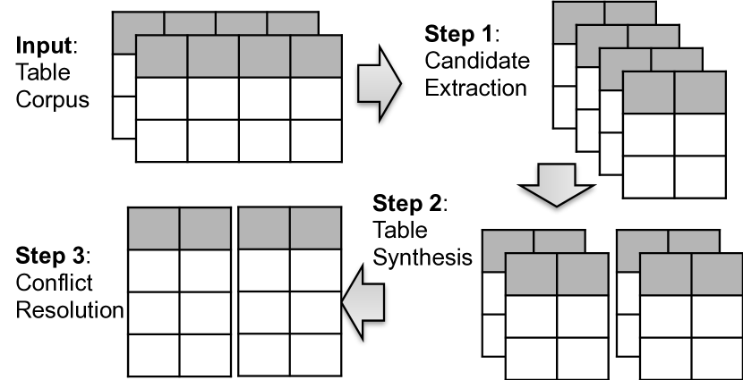
Our approach has three main steps, as shown in Figure 2.

Step 1: Candidate Extraction

This step starts by exhaustively extracting pairs of columns from all tables in the corpus as candidates for synthesis. For each table $T=\{C_{1},C_{2},...,C_{n}\}$ with $n$ columns, we can extract $2{{n}\choose{2}}$ such ordered pairs. However, many column pairs are not good candidate for mapping relationships because (1) for some column pair if the local relationship is already not functional, then it is unlikely to participate in true mappings; and (2) some table columns are of low quality and are not coherent enough (e.g., with mixed concepts). To address these issues, we use FD constraints as well as value-based co-occurrence statistics to prune away low-quality candidate tables.

Step 2: Table Synthesis

In this step, we judiciously synthesize two-column tables that describe the same relationship and are compatible with each other. The reason this is necessary is because many web tables and spreadsheets are for human consumption [30], and as a result contain only a subset of instances for the ease of browsing. Furthermore, one table in most cases mentions an entity by one name; synthesis helps to improve coverage of synonyms that are important for many applications.

Step 3: Conflict Resolution

Because results from table synthesis piece together many tables, some of which are bound to have erroneous values inconsistent with others, namely two pairs of values in the same mapping with the same left-hand-side value but different right-hand-side (thus violating the definition of mappings). These can often happen due to quality issues or extraction errors. We apply a post-processing step to resolve conflicts in synthesized mapping relationships to produce our final results.

3 Candidate Table Extraction

In this section we briefly describe the preprocessing of tables. Recall that in this work we focus on synthesizing binary mapping relationships. We start with two-column tables extracted from an existing table corpus. Given a table $T=\{C_{1},C_{2},...C_{n}\}$ with $n$ columns, we can extract binary tables with pairs of columns $\{(C_{i},C_{j})|i,j\in[n],i\neq j\}$, for a total of $2{{n}\choose{2}}$ such column pairs. For example, in Figure 7, we can conceptually extract all pairs of columns such as (Home Team, Away Team), (Home Team, Date), (Home Team, Stadium), (Home Team, Location), etc.

Because not all these pairs are meaningful mappings, we filter out candidates with a coherence-based filtering and a local FD based filtering.

Table 7: An example input table. Candidate two-column tables can be extracted using both PMI and FD filtering.

3.1 Column Filtering by PMI

When given a large table corpus (especially web tables), some tables are inevitably of low quality. Quality issues can arise because (1) columns may be mis-aligned due to extraction errors (especially for complicated tables like pivot table and composite columns); or (2) some table columns just have incoherent values.

In both of these cases, the resulting table column will appear to be “incoherent” when looking at all values in this column. For example, the last column Location in Table 7 have mixed and incoherent values. We would like to exclude such columns from consideration for mapping synthesis.

Therefore we measure the coherence of a table column based on semantic coherence between pairs of values. We apply a data-driven approach to define coherence based on co-occurrence statistics in a corpus. Let $s(u,v)$ be the coherence between two values $u$ and $v$. Define $\mathcal{C}(u)=\{C|u\in C,C\in T,T\in\mathcal{T}\}$ as the columns in the table corpus $\mathcal{T}$ containing value $u$, and define $\mathcal{C}(v)$ similarly. Clearly, if $\mathcal{C}(u)\cap\mathcal{C}(v)$ is a large set, it means $u$ and $v$ are co-occurring frequently (e.g., $u=$ USA and $v=$ Canada). Then they intuitively are highly related and thus should have a high semantic coherence score.

We use Point-wise Mutual Information (PMI) [14] to quantify the strength of co-occurrence as a proxy for coherence.

$$\text{PMI}(u,v)=\log\frac{p(u,v)}{p(u)p(v)}$$ (1)

Where $p(u)$ and $p(v)$ are the probabilities of seeing $u$ and $v$ from a total of $N$ columns in a table corpus $\mathcal{T}$, defined as $p(u)=\frac{|\mathcal{C}(u)|}{N}$, $p(v)=\frac{|\mathcal{C}(v)|}{N}$ and $p(u,v)=\frac{|\mathcal{C}(u)\cap\mathcal{C}(v)|}{N}$.

Example 4

Let $u=$USA and $v=$ Canada. Suppose $N=100M$ (there are a total of 100M columns), $|\mathcal{C}(u)|=1000$, $|\mathcal{C}(v)|=500$, and $|\mathcal{C}(u)\cap\mathcal{C}(v)|=300$ (individually, the two strings occur 1000 and 500 times respectively; together they co-occur 300 times). It can be calculated that PMI$(u,v)=4.78>0$, suggesting that they have high co-occurrence and strong semantic coherence.

We define coherence of two values, denoted by $s(u,v)$, as a normalized version of PMI called Normalized PMI (NPMI), which has a range of $[-1,1]$:

$$s(u,v)=\text{NPMI}(u,v)=\frac{\text{PMI}(u,v)}{-\log p(u,v)}$$

Using $s(u,v)$, the coherence score of a column $C=\{v_{1},v_{2},...\}$, denoted as $S(C)$, is simply the average of all pair-wise scores.

$$S(C)=\frac{\sum_{v_{i},v_{j}\in C,i<j}s(v_{i},v_{j})}{{{|C|}\choose{2}}}$$ (2)

We can then filter out a column $C$ if its coherence $S(C)$ is lower than a threshold.

Example 5

Table 7 is an example table with five columns. Column coherence computed using NPMI in Equation (2) would reveal that the first four columns all have high coherence scores, because values in these columns co-occur often in the table corpus.

The last column Location, however, has low coherence, because values in this column are mixed and do not co-occur often enough in other columns. We will remove this column when generating column pairs.

3.2 Column-Pair Filtering by FD

After removing individual columns with low coherence scores, we use the resulting table $T=\{C_{1},C_{2},...,C_{n}\}$ to generate binary tables with ordered column pairs $B(T)=\{(C_{i},C_{j})|$ $i,j\in[n],i\neq j\}$ as candidate tables. However, most of these two-column tables do not express meaningful mapping relationships, such as (Home Team, Away Team), and (Home Team, Date) in Table 7.

Since our goal is to produce mapping relationships, we apply local FD checking to prune away column pairs unlikely to be mappings. As discussed in Definition 3 we account for name ambiguity (like (Portland $\rightarrow$ Oregon) and (Portland $\rightarrow$ Maine)) by allowing approximate FD that holds for 95% of values.

Example 6

Continue with Example 5, we have pruned away the last column Location from Table 7 based on coherence scores. Four columns remain, for a total of $2{{4}\choose{2}}=12$ ordered column pairs. Only $2$ out of the $12$ column pairs satisfy FD, namely, (Home Team, Stadium) and (Stadium, Home Team).

We note that around $78\%$ candidates can be filtered out with these methods. The procedure used in this step can be found in Appendix A.

4 Table Synthesis

Using candidate two-column tables produced from the previous step, we are now ready to synthesize relationships. Recall that synthesis provides better coverage for instances (e.g., synonyms) as discussed in the introduction.

4.1 Compatibility of Candidate Tables

In order to decide what candidate tables should be stitched together and what should not, we need to reason about compatibility between tables.

Figure 3: Mappings from Wikipedia for country names and three types of country codes: IOC, FIFA, and ISO. The three have identical codes for many countries, but also different ones for many others (in red circles).

(a) $B_{1}$: IOC-(1)

(b) $B_{2}$: IOC-(2)

(c) $B_{3}$: ISO

Table 8: Example two-column binary tables for synthesis: (a) Countries and IOC codes, (b) Countries and IOC codes, where some countries use alternative synonyms compared to the first table, (c) Countries and ISO codes, where the code for some country can be different from the first two tables.

Positive Evidence for Compatibility

Let $B=\{(l_{i},r_{i})\}$ and $B^{\prime}=\{(l^{\prime}_{i},r^{\prime}_{i})\}$ be two binary relationships produced by the previous step, each with sets of (left, right) value pairs. If these two relations share many common value pairs, or $|B\cap B^{\prime}|$ is large, they are likely in the same relationship and compatible for synthesis.

Let $w^{+}(B,B^{\prime})$ be the positive compatibility between $B$ and $B^{\prime}$. We would like to use set-based similarity to quantify compatibility based on the overlap $|B\cap B^{\prime}|$. However, common metrics like Jaccard Similarity, defined as $\frac{|B\cap B^{\prime}|}{|B\cup B^{\prime}|}$, would not work because if one small relation is fully contained by another ($B\supset B^{\prime}$, $|B|\gg|B^{\prime}|$), the compatibility should intuitively be high, but the Jaccard Similarity score would actually be low.

Containment metrics would mitigate this issue, but Jaccard Containment is asymmetric – we want it to be symmetric because both the compatibility of $B$, $B^{\prime}$ and the compatibility of $B^{\prime}$, $B$ are essentially the same thing ($w^{+}(B,B^{\prime})$ = $w^{+}(B^{\prime},B)$). Given these we use a symmetric variant of Jaccard Containment called Maximum-of-Containment [8] for $w^{+}(B,B^{\prime})$:

$$w^{+}(B,B^{\prime})=\max\{\frac{|B\cap B^{\prime}|}{|B|},\frac{|B\cap B^{\prime}|}{|B^{\prime}|}\}$$ (3)

Example 7

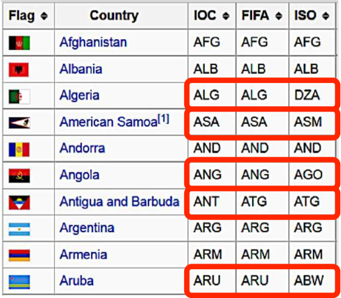
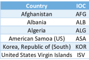
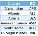
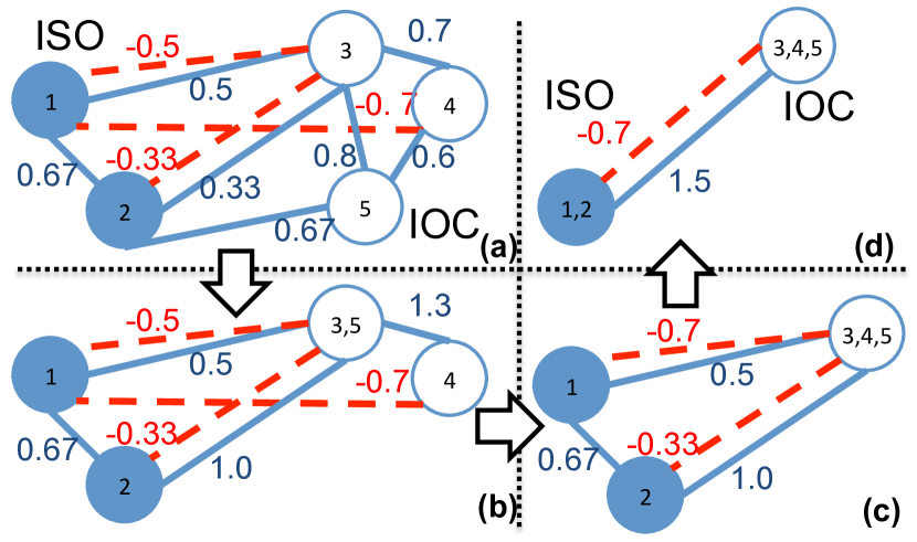
Table 8 shows three two-column candidate tables, $B_{1}$, $B_{2}$ and $B_{3}$, respectively. The first two are for the IOC code, while the last is for a different ISO code. All of these three are valid mappings but are for two different country-code standards, as explained in Figure 2.

Using Equation (3), we can compute the positive compatibility between each pair of tables. For example, we have $w^{+}(B_{1},B_{2})=\max\{\frac{3}{6},\frac{3}{6}\}=0.5$, because $|B_{1}\cap B_{2}|=3$ (the first three rows), suggesting that the two tables share a significant fraction of mappings and are likely to be compatible for synthesis.

Efficiency. Although conceptually compatibility scores can be computed for all pairs of candidates, in reality most tables share no common values, and will have a score of 0. A practical issue here is that given $N$ total candidate tables, we need to perform $O(N^{2})$ expensive containment computations. With millions of tables, this quadratic step is too expensive even for large Map-Reduce clusters.

In reality we observe that the scores for most pairs of tables are zero since they share no overlapping values at all. For example, Table 1(a) is about countries and Table 1(b) is about stock tickers. They have no overlaps in value-pairs, so both positive and negative weights are 0. Computing scores for these non-overlapping sets is clearly wasteful.

To address this problem, we use inverted-index-like regrouping in a Map-Reduce round to map all tables sharing at least some common value-pairs to the same partition, so that compatibility is computed only for pairs of tables within each partition. Specifically, we evaluate $w^{+}(B,B^{\prime})$ only if $B$ and $B^{\prime}$ share more than $\theta_{overlap}$ value pairs (both left and right values), and similarly we evaluate $w^{-}(B,B^{\prime})$ only if $B$ and $B^{\prime}$ share more than $\theta_{overlap}$ left-hand-side values. In practice, the number of non-zero weighted edges is much smaller than $N^{2}$. This optimization makes it possible to scale the pair-wise computation step to hundreds of millions of tables.

Approximate String Matching. In real tables, values from different tables often have slight variations, such as “Korea, Republic of” & “Korea Republic”, or “American Samoa” & “American Samoa (US)”. In practice, there are other extraneous information in table cells, such as the footnote mark “[1]” in the fourth row in Figure 2. These artificially reduce positive compatibility and in some cases increase negative compatibility between tables, which is undesirable.

To account for such minor syntactic variations, we use approximate string matching between cell values. Specifically, we measure the Edit Distance, denoted as $d_{ed}(v_{1},v_{2})$, between a pair of values $v_{1}$ and $v_{2}$. We treat $v_{1}$ and $v_{2}$ as a match if $d_{ed}(v_{1},v_{2})$ is smaller than a threshold $\theta_{ed}$. Here we use a fractional threshold defined as $\theta_{ed}=\min\{\lfloor|v_{1}|\cdot f_{ed}\rfloor,\lfloor|v_{2}|\cdot f_{ed}\rfloor\}$, which is dynamically determined based on the length of string $|v_{1}|$, $|v_{2}|$, and a fixed fractional value $f_{ed}$ (e.g., 0.2). We choose to use a fractional distance instead of an absolute distance, because the desired edit distance should change based on the length of values. For example, for short values such as “USA” or “RSA” (for South Africa), any absolute distance threshold $\geq 1$ would incorrectly match the two. Fractional threshold on the other hand would require an exact match for short strings like these. We further restrict the threshold to be within some fixed threshold $k_{ed}=10$ to safeguard false positives. Combining, we use $\theta_{ed}(v_{1},v_{2})=\min\{\lfloor|v_{1}|\cdot f_{ed}\rfloor,\lfloor|v_{2}|\cdot f_{ed}\rfloor,k_{ed}\}$.

Example 8

We continue with Example 7 in Table 8. When using approximate matching for positive compatibility, $w^{+}(B_{1},B_{2})$ will now be updated to $\max\{\frac{4}{6},\frac{4}{6}\}=0.67$. This is because in addition to the first three matching rows between $B_{1}$ and $B_{2}$, now the fourth row “American Samoa” and “American Samoa (US)” will also be considered as a match, as the Edit Distance between the two values is 2 (ignoring punctuations), which is no greater than $\theta_{ed}=\min\{\lfloor 13\cdot 0.2\rfloor,\lfloor 15\cdot 0.2\rfloor,10\}=2$.

Efficiency. There are hundreds of millions of table pairs for which we need to compute compatibility. Let $m$ and $n$ be the numbers of values in a pair of tables. For each pair we need to make $O(nm)$ approximate string comparisons, each of which is in turn $O(|v_{1}||v_{2}|)$ when using conventional dynamic programming on the full matrix. This is too expensive even for production Map-Reduce clusters.

Our observation is that the required edit distance threshold $\theta_{ed}$ is small in most cases. So using ideas similar to the Ukkonen’s algorithm [35], we only compute DP on the narrow band in the diagonal direction of the matrix, which makes it $O(\theta_{ed}\cdot\min\{|v_{1}|,|v_{2}|\})$. Since $\theta_{ed}$ is small it makes this step feasible. Pseudo-code of this step can be found in Appendix B.

Synonyms. In some cases, synonyms of entity names may be available, e.g., using existing synonym feeds such as [10]. If we know, for instance, “US Virgin Islands” and “United States Virgin Islands” are synonyms from external sources, we can boost positive compatibility between $B_{1}$ and $B_{2}$ in Table 8 accordingly. We omit discussions on possible lookup-based matching in the interest of space.

Negative Evidence for Incompatibility

Positive evidence alone is often not sufficient to fully capture compatibility between tables, as tables of different relationships may sometimes have substantial overlap. For example, it can be computed that the positive compatibility between $B_{1}$ in Table 4(a) and $B_{3}$ Table 4(c) is $\max\{\frac{3}{6},\frac{3}{6}\}=0.5$ (the first, second and fifth rows match). Given the high score, the two will likely merge incorrectly (note that one is for IOC code while the other is for ISO). This issue exists in general when one of the columns is short and ambiguous (e.g. codes), or when one of the tables has mixed values from different mappings (e.g., both city to state and city to country).

We observe that in these cases the two tables actually also contain conflicting value pairs, such as the third and fourth row in the example above where the two tables have the same left-hand-side value, but different right-hand-side values. This violates the definition of mapping relationship, and is a clear indication that the two tables are not compatible, despite their positive scores.

We thus introduce a negative incompatibility between tables. Given two tables $B$ and $B^{\prime}$, define their conflict set as $F(B,B^{\prime})=\{l|(l,r)\in B,(l,r^{\prime})\in B^{\prime},r\neq r^{\prime}\}$, or the set of values that share the same left-hand-side but not the right-hand-side. For example, between $B_{1}$ in Table 4(a) and $B_{3}$ Table 4(c), (Algeria, ALG) and (Algeria, DZA) is a conflict.

To model the (symmetric) incompatibility between two tables $B$ and $B^{\prime}$, we define a negative incompatibility score $w^{-}(B,B^{\prime})$ similar to positive compatibility in Equation (3):

$$w^{-}(B,B^{\prime})=-\max\{\frac{|\textit{F}(B,B^{\prime})|}{|B|},\frac{|\textit{F}(B,B^{\prime})|}{|B^{\prime}|}\}$$ (4)

Example 9

We continue with Example 8 in Table 8. As discussed earlier, the positive compatibility between $B_{1}$ in Table 4(a) and $B_{3}$ in Table 4(c) is $\max\{\frac{3}{6},\frac{3}{6}\}=0.5$, which is substantial and will lead to incorrect merges between two different relationships (IOC and ISO).

Using negative incompatibility, we can compute $w^{-}(B_{1},B_{3})$ as $-\max\{\frac{3}{6},\frac{3}{6}\}=-0.5$, since the third, forth and sixth rows conflict between the two tables, and both tables have 6 rows. This suggests that $B_{1}$ and $B_{3}$ have substantial conflicts, indicating that a merge will be inappropriate.

In comparison, for $B_{1}$ in Table 4(a) and $B_{2}$ in Table 4(b), which talk about the same relationship of IOC, their conflict set is empty and $w^{-}(B_{1},B_{2})=0$, indicating that we do not have negative evidence to suggest that they are incompatible.

4.2 Problem Formulation for Synthesis

We use a graph $G=(\mathcal{B},E)$ to model candidate tables and their relationships, where $\mathcal{B}$ is the union of all binary tables produced in the preprocessing step in Section 3. In $G$ each vertex represents a table $B\in\mathcal{B}$. Furthermore, for each pairs of vertices $B,B^{\prime}\in\mathcal{B}$, we use compatibility scores $w^{+}(B,B^{\prime})$ and incompatibility scores $w^{-}(B,B^{\prime})$ as the positive and negative edge weights of the graph.

Example 10

Given the tables $B_{1}$, $B_{2}$ and $B_{3}$ in Table 8, we can represent them and their compatibility relationships as a graph as in Figure 4(a).

As discussed in Example 8, the positive compatibility between $w^{+}(B_{1},B_{2})=0.67$, which is shown as solid edge with positive weight in this graph. Similarly we have negative edge weights like $w^{-}(B_{1},B_{3})=-0.5$ as discussed in Example 9. This graph omits edges with a weight of 0, such as $w^{-}(B_{1},B_{2})$.

Since we need to synthesize compatible tables into larger mapping relationships, in the context of graph $G$ we need to group compatible vertices/tables together. This naturally corresponds to a partitioning $\mathcal{P}=\{P_{1},P_{2},...\}$ of $\mathcal{B}$, where each $P_{i}\subseteq\mathcal{B}$ represents a subset of tables that can be synthesized into one relationship. Since different partitions correspond to distinct relationships, the partitioning should be disjoint ($P_{i}\cap P_{j}=\emptyset,i\neq j$), and they should collectively cover $\mathcal{B}$, or $\bigcup_{P\in\mathcal{P}}{P}=\mathcal{B}$.

Intuitively, there are many ways to partition $\mathcal{B}$ disjointly, but we want to find a good partitioning that has the following desirable properties: (1) compatible tables are grouped together as much as possible to improve coverage of individual mapping relationships; and (2) incompatible tables should not be placed in the same partition.

We translate these intuitive requirements into an optimization problem. First, we want each partition $P$ to have as many compatible tables as possible. Let $w^{+}(P)$ be the sum of positive compatibility in a partition $P$:

$$w^{+}(P)=\sum_{B_{i},B_{j}\in P,i<j}w^{+}(B_{i},B_{j})$$

We want to maximize the sum of this score across all partitions, or $\sum_{P\in\mathcal{P}}{w^{+}(P)}$. This is our optimization objective.

On the other hand, we do not want to put incompatible tables with non-trivial $w^{-}$ scores, such as $B_{1}$ and $B_{3}$ in Example 10, in the same partition. Since we disallow this to happen, we treat edges with negative scores $w^{-}$ below a threshold $\tau$ as hard-constraints. Note that a negative threshold $\tau$ (e.g., $-0.2$) is used in place of 0 because we do not over-penalize tables with slight inconsistency due to minor quality and extraction issues. We ignore the rest with insignificant negative scores by essentially forcing them to 0. Let $w^{-}(P)$ be the sum of substantial negative weights in $P$ defined below.

$$w^{-}(P)=\sum_{B_{i},B_{j}\in P,w^{-}(B_{i},B_{j})<\tau}w^{-}(B_{i},B_{j})$$

We use this as a constraint of our formulation – we want no edges in the same partition to have substantial conflicts, or, $w^{-}(P)=0,\forall P\in\mathcal{P}$.

Putting these together, we formulate table synthesis as follows.

Problem 11 (Table Synthesis)

max $$\sum_{P\in\mathcal{P}}{w^{+}(P)}$$ (5)

s.t. $$\sum_{P\in\mathcal{P}}{w^{-}(P)}=0$$ (6)

$$P_{i}\bigcap P_{j}=\emptyset,\quad~{}\quad\forall P_{i}\neq P_{j}$$ (7)

$$\bigcup_{P\in\mathcal{P}}P=\mathcal{B}$$ (8)

By placing compatible tables in the same partition, we score more in the objective function in Equation (5), but at the same time Equation (6) guarantees that no conflicting negative edge can be in the same partition. Equation (7) and (8) are used to ensure that $\mathcal{P}$ is a proper disjoint partitioning.

Figure 4: Graph representation of candidate tables. Solid vertices on the left represent tables for ISO codes; hollow vertices on the right represent tables for IOC codes. Furthermore, solid edges indicate positive compatibility, while dashed edges indicate negative incompatibility. Edges with weight of 0 are omitted on the graph.

Example 12

We revisit the example in Figure 4(a). Using the formulation above, it can be verified that the best partitioning is $\{\{B_{1},B_{2}\},$ $\{B_{3},B_{4},B_{5}\}\}$, which groups two ISO tables and three IOC tables into separate partitions. This partitioning has a total score of $2.77$ based on Equation (5), without violating constraints in Equation (6) by not placing negative edges in the same partition.

It is worth noting that existing techniques like schema matching [31] only consider positive similarity (because FD do not generally hold in tables), and as a result merge all 5 tables in this example, producing results of low quality.

Theorem 13

The problem Table-Synthesis is NP-hard.

We prove this using a reduction from graph multi-cut. There also exists a trichotomy of complexity depending on the number of negative edges in the graph. A proof of the hardness can be found in Appendix C.

What is interesting is that there exists a trichotomy result in terms of complexity [17]. Specifically, if the graph has exactly 1 negative edge, the problem is equivalent to min-cut, max-flow because we can make the pair of vertices incident to the negative edge as source and sink, respectively. When there exist 2 negative edges, the problem can be solved in polynomial time using results from [39]. In the more general case when there are no fewer than $3$ negative edges, the problem becomes NP-hard.

Despite the hardness, there is a $O(\log N)$-approximation algorithm for the loss-minimization version of Problem 11. Specifically, the loss-minimization version of the problem can be written as follows, which minimizes the positive edge weights that are lost as a result of the partitioning that disconnects all the negative edges.

Problem 14 (Loss Minimization)

min $$\sum_{B\in P_{i},B^{\prime}\in P_{j},i\neq j}{w^{+}(B,B^{\prime})}$$ (9)

s.t. $$\sum_{P\in\mathcal{P}}{w^{-}(P)}=0$$ (10)

$$P_{i}\bigcap P_{j}=\emptyset,\quad~{}\quad\forall P_{i}\neq P_{j}$$ (11)

$$\bigcup_{P\in\mathcal{P}}P=\mathcal{B}$$ (12)

Using standard embedding techniques, we can encode partition decisions using distance variables $d_{ij}$. $d_{ij}=0$ if vertices $B_{i}$ and $B_{j}$ are in the same partition, and $d_{ij}=1$ if they are in different partitions. This produces the following formulation.

Problem 15 (Embedding)

min $$\quad\sum{w^{+}(B_{i},B_{j})\cdot d_{ij}}$$

s.t. $$\quad{}d_{ij}+d_{jk}\geq d_{ik},\quad{}\forall i,j,k$$ (13)

$$\quad{}d_{ij}=d_{ji}$$ (14)

$$\quad{}d_{ij}\in\{0,1\}$$ (15)

$$\quad{}d_{ij}=1,\qquad{}\quad~{}\quad\forall w^{-}(B_{i},B_{j})<\tau$$ (16)

This problem is known to be APX-hard [16]. Using classical techniques including LP-relaxation and region-growing for randomized rounding [5, 19, 36], it is possible to produce $O(\log N)$ approximation. More discussions of this can be found in Appendix D in the interest of space.

Such an approximation scheme requires to model each pair of vertices as a decision variable $d_{ij}$, and then solve the associated LP before applying randomized rounding. While it may be practical for problems of moderate sizes, we are dealing with graphs with millions of vertices, where solving an LP with a quadratic number of variables is clearly infeasible.

As a result, we use an efficient heuristic to perform greedy synthesis. Specifically, we initially treat each vertex as a partition. We then iteratively merge a pair of partitions $(P_{1},P_{2})$ that are the most compatible to get a new partition $P^{\prime}$, and update the remaining positive/negative edges.The algorithm terminates when no partitions can be merged. Pseudo-code of this procedure can be found in Appendix E.

Efficiency. While the procedure above appears straightforward for graphs that fit in a single machine, scaling to large graphs on Map-Reduce is not straightforward. We use a divide-and-conquer approach to first produce components that are connected non-trivially by positive edges on the full graph, and then look at each subgraph individually. More discussions on this step can be found in Appendix F.

Example 16

Figure 4 shows how Algorithm 3 works on a small graph. The algorithm first merges $\{B_{3}\}$ and $\{B_{5}\}$ to get Figure 4b because Edge $(\{B_{3}\},\{B_{5}\})$ has the greatest weight. The weight of Edge $(\{B_{2}\},\allowbreak\{B_{3},B_{5}\})$ changes as $w^{+}(\{B_{2}\},\allowbreak\{B_{3},B_{5}\})\Leftarrow w^{+}(\{B_{2}\},\{B_{3}\})+w^{+}(\{B_{2}\},\{B_{5}\})$. The weight of Edge $(\{B_{4}\},\allowbreak\{B_{3},B_{5}\})$ also changes similarly.

The algorithm then merges $\{B_{3},B_{5}\}$ and $\{B_{4}\}$ to get Figure 4c and finally combines $\{B_{1}\}$ and $\{B_{2}\}$ to get Figure 4d. The algorithm stops because of the negative weight between $\{B_{1},\allowbreak B_{2}\}$ and $\{B_{3},B_{4},B_{5}\}$.

Conflict Resolution

Figure 5: A real table with errors that can cause conflicts.

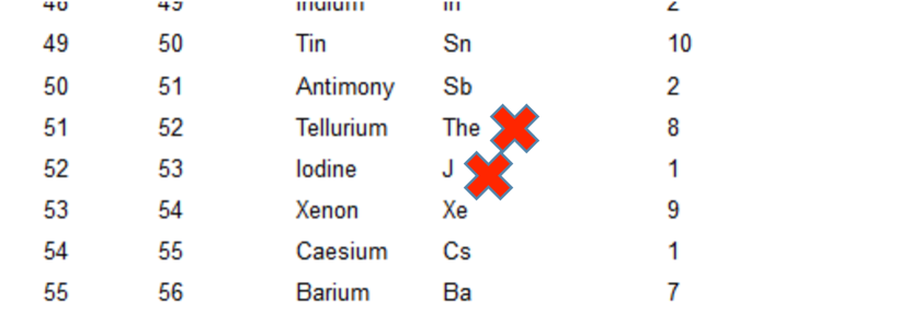
We observe that synthesized relations often have conflicts that require post-processing. Specifically, when we union all tables in the same partition together, there will be a small fraction of rows that share the same left-hand-side value, but have different right-hand-side values. This could be due to quality issues in the original input tables, such as the example in Figure 5 that has incorrect chemical symbols for two of the rows (the symbol of Tellurium should be Te and Tellurium should be I). Quality issues like this are actually common in large corpus, and manifest themselves as inconsistent mappings in synthesized results. Since the majority of tables in the partition should agree with the ground-truth mapping, we resolve conflicts by removing the least number of low-quality tables, such that the resulting partition has no conflicts.

Let $P$ be a partition with candidate tables $\{B_{1},B_{2},...\}$, each of which is a set of value pairs $B_{i}=\{(l,r)\}$. Recall that in Section 4.1 we define a conflict set $F(B,B^{\prime})$ to be $\{l|(l,r)\in B,(l,r^{\prime})\in B^{\prime},r\neq r^{\prime}\}$. We can again leverage synonyms and do not treat $(l,r),(l,r^{\prime})$ as conflicts if $(r,r^{\prime})$ are known to be synonyms.

Now we want to find out the largest subset $P_{T}\subseteq\mathcal{P}$ such that no two tables in $P_{T}$ conflict with each other, which can be formulated as follows.

Problem 17 (Conflict Resolution)

max $$\left|\bigcup_{B_{i}\in P_{T}}B_{i}\right|$$

s.t. $$F(B_{i},B_{j})=\emptyset,\quad\forall B_{i},B_{j}\in P_{T}$$ (17)

The objective is to include as many value pairs as possible, under the constraint that no pairs of tables in the selected subset $P_{T}$ can have conflict.

This problem is NP-hard (reduction from Independent Set). So we iteratively find and remove a value pair that conflicts with the most other value pairs. Pseudo-code of this procedure can be found in Appendix H.

Table Expansion

Another potential issue is that for large mapping relationships such as (airport-name, airport-code) that has more than 10K instances, synthesized tables may still miss values that are unpopular with little or no presence in web tables. We expand synthesized results that are robust “cores”, using trustworthy sources such as data.gov or spreadsheet files (.xlsx). Appendix I gives more details for this optional step.

We note that there are many existing methods for conflict resolution [28] that can conceptually be applied to the post-processing step, and it is interesting to explore their applicability. Because we do not consider this post-processing step to be our key contribution, and we include this step here for completeness, we do not perform an exhaustive comparison.

4.3 Synthesized Mappings for Curation

While the synthesized mappings produced by our algorithm are generally of high quality, for many applications a very high precision is required. For example, for commercial spreadsheet software like Excel, any error introduced by black-box algorithms can be hard to detect by users, but has damaging consequences and thus unacceptable. In such settings, our approach of pre-computing all candidate mappings from table corpora allows humans to inspect and curate these mappings to ensure very high accuracy. High-quality mappings produced by automatic algorithms can greatly reduce the effort required by human curators.

It is interesting to note that synthesized results we produce have a natural notion of importance/popularity. Specifically, for each synthesized mapping, we have statistics such as the number of web domains whose tables contributed to this mapping, and how many raw tables are synthesized in the same cluster, etc. Such statistics are very well correlated to the importance of the mapping, because the more it occurs in the table corpus, the more likely it is frequently used and important. This property makes results produced by our approach amenable to human curation – instead of looking at a full corpus with millions of tables, one just needs to look at synthesized results popular enough.

In our experiments using a web corpus, we only use about 60K synthesized mappings from at least 8 independent web domains, which is orders of magnitude less than the the number of input tables. Additional filtering can be performed to further prune out numeric and temporal relationships.

While most mappings are static that rarely change, some are temporal in nature and may be changing over time. But like knowledge-bases used by search engines that also face the same “data freshness” problem (e.g., when a famous actor gets newly married, the knowledge-card used by search engines should reflect that new fact within a short period of time), algorithms and human curation can for the most part mitigate this problem (e.g., regularly refreshing the data by rerunning the pipeline and alert human curator for changes). Additional mechanisms include crowd-sourcing that allows users to report/flag stale values for them to be corrected. We would like to note that because a large fraction of the mappings harvested are static in nature, a one-shot curation of just these mappings can already produce significant values to a variety of applications.

5 Experiments

5.1 Experimental Setup

Table Corpus

We use two table corpora for our evaluation.

The first table corpus, henceforth denoted as Web, has over 100 million tables crawled and extracted from the public web. These tables cover diverse domains of interests.

The second table corpus, denoted as Enterprise, has about 500K tables extracted from spreadsheets files crawled from the intranet of a large IT company.

Computing Environment

We implemented algorithms described in this paper as Map-Reduce programs. We ran our jobs in a large Map-Reduce cluster, alongside with other production jobs. Our input for Web has about 223M two-column tables with a size of over 200GB.

Benchmarks

We have built a benchmark dataset to evaluate our framework on Web table corpus . This benchmark dataset contains 80 desirable mapping relationships that we manually curated. These relationships are collected from two sources.

list of countries and capitals	list of pokemons and categories
list of car models and makes	list of amino acids and symbols

Figure 6: Example queries with “list of A and B”

• Geocoding: We observe that geography is a common domain with rich mapping relationships that are often used in auto-join and auto-correction scenarios. Examples here include geographical and administrative coding such as country code, state code, etc. So we take 14 cases from a Wikipedia list of geocoding systems. We omit codes that are impossible to enumerate such as military grid reference system, and ones not completely listed on Wikipedia such as HASC code. Figure 7 lists all cases we take.

• Query Log: We sample queries of the pattern “list of A and B” in Bing query logs that search for mapping relationships. Figure 6 shows a few examples with true mappings.

FIPS 5-2	ISO 3166-1 Alpha-3
FIPS 10-4	ISO 3166-1 Numeric
IANA Country Code	ITU-R Country Code
IATA Airport Code	ITU-T Country Calling Code
ICAO Airport Code	MARC Country Code
IOC Country Code	NUTS (EU)
ISO 3166-1 Alpha-2	SGC Codes (Canada)

Figure 7: Geocoding Systems

For Web, after selecting mapping relationships, we curate instances for each relationship, by combining data collected from web tables as well as knowledge bases. Specifically, we find a group of tables for each relationship, and then manually select high-quality ones to merge into the ground truth. Finally we combine these high-quality web tables with instances in Freebase and YAGO if they have coverage. Note that the resulting mapping relationships have rich synonyms for the same entity (e.g., as shown in Table 6), as well as more comprehensive coverage for instances. Constructing such a benchmark set, and ensuring its correctness/completeness is a time-consuming process. We intend to publish this benchmark set online to facilitate future research in this area.

Enterprise is more difficult to benchmark because of the difficulty in ensuring completeness of instances in certain mappings – the ground truth may be in master databases for which we have no access (e.g., employee and login-alias). Nevertheless, we built 30 best effort benchmark cases. Recall results on these tests should be interpreted as relative-recall given the difficulty to ensure completeness.

Metrics

We use the standard precision, recall and f-score to measure the performance. Let $B^{*}=\{(l^{*},r^{*})\}$ be a ground truth mapping, and $B=\{(l,r)\}$ be a synthesized relationship for which we want to evaluate its quality. The precision of $B$ is defined as $\frac{|B\cap B^{*}|}{|B|}$, the recall is $\frac{|B\cap B^{*}|}{|B^{*}|}$, and the f-score is $\frac{2\text{precision}\cdot\text{recall}}{\text{precision}+\text{recall}}$.

Methods compared

We compare the following methods.

• UnionDomain. Ling and Halevy et al. [30] propose to union together tables within the same website domain, if their column names are identical but row values are disjoint. We apply this technique by essentially grouping tables based on column names and domain names. We evaluate the resulting union tables against each benchmark case by picking the union table with the highest F-score.

• UnionWeb. Noticing that only union-ing tables in the same domain may be restrictive and missing instances for large relationships, we extend the previous approach to also merge tables with the same column names across the web, and evaluate all benchmark cases like above. This is a variant of UnionDomain.

• Synthesis. This is our approach that synthesizes mapping relationships as described in Section 4.

• SynthesisPos. This is the same as Synthesis except that it does not use the negative signals induced by FDs. This helps us to understand the usefulness of negative signals.

• WiseIntegrator [22, 23]. This is a representative method in a notable branch in schema matching that collectively matches schemas extracted from Web forms. It measures the similarity between candidates using linguistic analysis of attribute names and value types, etc., and performs a greedy clustering to group similar attributes.

• SchemaCC. In this method, we mimic pair-wise schema matchers that use the same positive/negative similarity as our approach. Because match decisions are pair-wise, we aggregate these to a group-level based on transitivity (e.g., if table A matches B and B matches C, then A also matches C). This is implemented as connected components on very large graphs, where edges are threshold based on a weighted combination of positive/negative scores. We tested different thresholds in the range of $[0,1]$ and report the best result.

• SchemaPosCC. This is the same as SchemaCC but without negative signals induced by FDs, since they are not explored in the schema matching literature. We again test thresholds in $[0,1]$ and report the best number.

• Correlation [12]. In this method, we again mimic pair-wise schema matchers with the same positive/negative scores as Synthesis. Instead of using connected components for aggregation as in SchemaCC above, here we instead use the correlation clustering that handles graphs with both positive or negative weights. We implement the state-of-the-art correlation clusterin on map-reduce [12], which requires $O(\log|V|\cdot\Delta^{+})$ iterations and takes a long time to converge ($|V|$ is the number of vertices of the graph and $\Delta^{+}$ is the maximum degree of all vertices). We timeout after $20$ hours and evaluate the results at that point.

• WikiTable. Wikipedia has many high-quality tables covering various domains, many of which have mapping relationships. To understand the quality of using raw tables instead of performing synthesis, we also evaluate each benchmark case by finding best pair of columns in a Wikipedia table that has the highest in F-score.

• WebTable. This method is very similar to the previous WikiTable, but use all tables in the Web corpus instead of just Wikipedia ones.

• Freebase. Freebase [7] is a well-known knowledge base that has been widely used. We obtained its RDF dump and extract relationships by grouping RDF triples by their predicates. We treat the subject $\rightarrow$ object as one candidate relationship, and the object $\rightarrow$ subject as another candidate.

• YAGO. YAGO [34] is another public knowledge base that is extensively used. We process a YAGO data dump similar to Freebase, by grouping YAGO RDF triples using their predicates to form subject-object and object-subject relationships.

Note that in all these cases, we score each benchmark case by picking the relationship in each data set that has the best f-score. This is favorable to all the methods – a human who wishes to pick the best relationship to be used as mappings, and who could afford to inspect all these tables, would effectively pick the same tables.

Figure 8: Average f-score, precision and recall comparison.

5.2 Quality Comparison

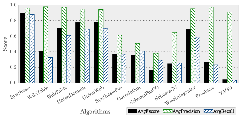
Figure 8 shows the average f-score, precision and recall across all 80 benchmark cases in the Web benchmark for all methods compared. Synthesis scores the best in average recall (0.88) and f-score (0.90), while WikiTable has the best average precision (0.98) .

In comparison, using only raw tables from WikiTable with no synthesis has high precision but low recall, because not only are certain instances and synonyms missing (these tables tend to be short for human consumption), many relationships are also missing altogether from WikiTable. So the approach of manually going over high-quality WikiTable to curate mapping relationships is unlikely to be sufficient.

The WebTable approach uses raw tables similar to WikiTable, but considers tables not limited to the Wikipedia domain and thus has substantially better recall. While the precision of WebTable and Synthesis are comparable, the recall of Synthesis is substantially higher (0.88 vs. 0.32). Despite this, we want to note that the setup of this comparison of is very favorable for WebTable – we select the best table among the hundreds of millions of raw tables in WebTable, whereas in Synthesis we only use relations synthesized from over 8 website domains that is three orders of magnitude less (Section 4.3). Because it is not possible for human to go over millions of tables to pick useful mappings in practice, WebTable only provides an upper-bound of what can be achieved and not really a realistic solution.

UnionDomain and UnionWeb synthesize tables based on table column names and domain names. The recall of these two approaches is considerably better than WikiTable and WebTable, showing the benefit of performing table synthesis. However, this group of approaches merge tables only based on column names, which are known to be uninformative and undescriptive in many cases. We observe that when applied to the whole web, this often leads to over-grouping and under-grouping. The overall f-scores of these approaches are the best among all existing methods, but still lag behind Synthesis, which uses values that are more indicative of table compatibility.

SynthesisPos uses the same algorithm as Synthesis but does not consider the negative incompatibility induced by FDs. It is interesting to observe that result quality suffers substantially, which underlines the importance of the negative signals.

SchemaCC performs substantially worse than Synthesis. Recall that it uses the same positive/negative signals, but aggregate pair-wise match decisions using connected components. This simple aggregation tends to over-group and under-group different tables, producing undesirable table clusters.

SchemaPosCC ignores the negative signals used in SchemaCC, since FD-induced negative signals are not explored in schema matching. Unsurprisingly, result quality drops even further.

Correlation is similar to SchemaCC that also mimics schema matchers with same signals, but aggregate using correlation clustering. Overall, its f-score is better than SchemaCC, but is still worse than Synthesis. We think there are two main reasons why it does not work well. First, at the conceptual level, the objective of correlation clustering is the sum of positive and negative edges. Because the number of table pairs that would be in different clusters far exceeds the ones that should be in the same clusters, making negative edges dominate the objective function. However, in our problem, we should actually only care about whether tables in the same clusters correspond to the identical mapping, which are the intra-cluster positive edges that are more precisely modeled in our objective function. Second, a shortcoming of the parallel-pivot algorithm [12] is that it only looks at a small neighborhood for clusters (i.e. one-hop neighbors of cluster centers) for efficiency. When small tables in the same mapping form a chain of connected components, looking at the immediate neighborhood of a pivot (cluster center) will misses most other tables, producing results with low recall.

We implemented the collective schema-matching method WiseIntegrator. It performs reasonably well but still lags behind Synthesis, mainly because of the difference in how scores are aggregated to produce holistic matches.

Please see Appendix J and K for more analysis on the experimental results.

5.3 Run-time Comparison

We analyze the the complexity of our approach in this section. The basic input of our problem is a graph $G=(V,E)$ where $V$ represents candidate tables and $E$ represents their similarity. The most expensive part of our algorithm is in table synthesis (Step 2) that computes edge similarity and performs iterative grouping.

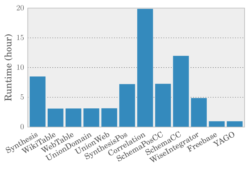
Figure 10 compares the runtime of all approaches. Knowledge bases are the most efficient because it amounts to a lookup of the relation with the highest f-score among all relations. WikiTable, WebTable, UnionDomain, UnionWeb, and WiseIntegrator are all relatively efficient but requires scans of large table corpus. Our approach Synthesis usually finishes within 10 hours (e.g., using parameters suggested here). Correlation is clearly the slowest, as correlation clustering converges very slowly even using the state-of-the-art parallel implementation on map-reduce [12].

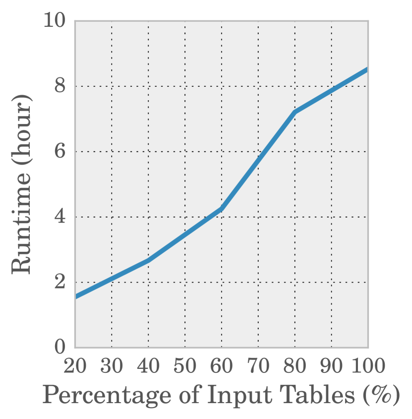
To test scalability of the proposed method, we sample $\{20\%,40\%,60\%,80\%\}$ of the input data and measures execution time, as shown in Figure 10. The complexity of the algorithm depends on the number of edges $|E|$. In the worst case $|E|$ can be quadratic to the number of tables $|V|$, but in practice $|E|$ is usually almost linear to $|V|$ due to edge sparsity. Figure 10 suggests that the algorithm scales close to linearly to the input data, which is encouraging as it should also scale to even larger data sets with billions of tables.

Figure 9: Runtime.

Figure 10: Scalability.

5.4 Sensitivity Analysis

We analyze the effect of parameters used in Synthesis.

• $\theta$. We use $\theta$ as a parameter when defining approximate mapping relationship, which is empirically set as $95\%$. When we vary $\theta$ between $93\%$ and $97\%$, the number of resulting mappings change very little (by up to $1\%$). We have also reverse-engineered by calculating the degree of approximation in desirable ground truth mappings (e.g. Springfield $\rightarrow$ Illinois and Springfield $\rightarrow$ Texas will create a violation). $95\%$ is sufficient to ensure that desired mappings will not be pruned incorrectly in almost all cases.

• $\tau$. This parameter controls when we determine two candidates conflict. Our results suggest that the quality is generally insensitive to small $\tau$. The performance peaks at around $-0.05$. In our other experiments we actually used $\tau=-0.2$ that also produces good quality.

• $\theta_{overlap}$ is a parameter for efficiency that determines the number of pruned edges $|E|$ in our graph. As $\theta_{overlap}$ increases, $|E|$ drops quickly. The quality of resulting clusters are insensitive to $\theta_{overlap}$.

• $\theta_{edge}$. We make $\theta_{edge}$ the threshold to filter out edges with insignificant positive weight. Our experiment suggests that $\theta_{edge}=0.85$ has the best performance.

5.5 Experiments on Enterprise

As we discussed earlier, unlike the Web domain where a large fraction of ground truth mappings can be constructed using common sense knowledge and online data sources, the ground truth mappings in the Enterprise domain is difficult to build. We are not familiar with many enterprise-specific data values and encodings in this corpus, which makes ensuring completeness and correctness of these mappings difficult.

We build $30$ benchmark cases with best effort to ensure completeness (for some mappings the ground truth may be in master databases we have no access to). To put the quality numbers in perspective, we compare Synthesis with single-table based EntTable, which is similar to WebTable in Web. As Figure 11 suggests that Synthesis achieve significantly higher recall by merging small tables. Its precision is also high by avoiding merging conflicting content.

	Synthesis	EntTable
Avg. (F-score, Prc., Rcl.)	(0.96, 0.96, 0.97)	(0.84, 0.99, 0.79)

Figure 11: Comparison with the alternative on Enterprise

Figure 12 shows some examples of mapping relationships produced. A large fraction of relationships are indeed important mappings, such as (product-family $\rightarrow$ code), (profit-center $\rightarrow$ code), (data-center $\rightarrow$ region), etc. Most of these results are well-structured and look consistent (shown in the right column of Figure 12), which is a good indication that results produced are of high quality.

Just like in the Web domain, applications equipped with these mapping relationships and some human curation can perform intelligent operations such as auto-join as discussed earlier. We note that these mappings are specific to this enterprise in question. Using tables to build such relationships would be the only reasonable choice, since alternatives like knowledge bases would not exist in enterprise domains.

Inspecting the results produced in Enterprise does reveal interesting issues. For example, we observe that for certain mapping relationships, the results are of low quality with mixed data values and meta-data values (e.g., column headers). It turns out that in spreadsheets, tables with complex structures such as pivot tables are popular. These complex tables are usually not flat relational tables that create difficulty for correct extraction.

Overall, given that rich mappings are produced for a completely different  Enterprise corpus, we believe that this exercise shows the promise of the Synthesis approach to generalize and produce mappings by just using a corpus of tables as input.

5.6 Effect of Conflict Resolution

Conflict resolution improves the f-score for 48 out of the 80 cases tested. On average, the precision increases from $0.903$ to $0.965$, while the average recall only dips slightly from $0.885$ to $0.878$. Such improvements shows that this post-processing step is useful in removing inconsistent value pairs without affecting coverage.

Cases such as (state $\rightarrow$ capital) see the biggest improvement. These relationships tend be confused with other relationships that disagree only on a small number of values. For example, the relationship (state $\rightarrow$ capital) tends to be confused with (state $\rightarrow$ largest-city) with only minor disagreements such as Washington and Olympia vs. Washington and Seattle. These conflicting value pairs will get mixed into results because for some subset of values there may not be sufficient incompatibility to prevent merges from happening. The conflict resolution step helps to prune away such incorrect values.

We compare our conflict resolution with majority voting. The proposed approach has a slightly higher f-score than majority voting. Appendix K has detailed results comparing the f-scores.

Mapping Relationship	Example Instances
(product-family, code)	(Access, ACCES),
	(Consumer Productivity, CORPO), …
(profit-center, code)	(P10018, EQ-RU - Partner Support),
	(P10021, EQ-NA - PFE CPM), …
(industry, vertical)	(Accommodation, Hospitality),
	(Accounting, Professional Services), …
(ATU, country)	(Australia.01.EPG, Australia),
	(Australia.02.Commercial, Australia), …
(data-center, region)	(Singapore IDC, APAC),
	(Dublin IDC3, EMEA), …

Figure 12: Example mapping relationships and values, from the enterprise spreadsheets corpus

6 Related Work

Ling and Halevy et al. studied the problem of stitching together web tables from the same domain based on column names [30]. When adapting this technique to generate mapping relationships for the whole Web, however, it tends to lead over-grouping and low-quality mappings (as we show in the experiments), because column names are often undescriptive and too generic to be indicative of the true meanings [15] (e.g., column names like code and name are common).

Knowledge bases such as Freebase [7], and YAGO [34] curate important entity-relationships, some of which may be mapping relationships. However, the coverage of knowledge bases is low as they often miss important mappings. For instance, YAGO has none of the example mappings listed in Table 1, while Freebase misses two (stock and airport). For mappings that do exist in knowledge bases, there are typically no or very few synonyms such as ones listed in Table 6. Lastly, knowledge bases are expensive to build, yet their mappings only cover the public Web domain, and does not generalize to other domains such as enterprises.

There is a long and fruitful line of research on schema matching [31] that can suggest semantic correspondence between columns for human users. These matching relationships provide useful information about positive compatibility between tables. However, using only positive signals of compatibility are insufficient for an unsupervised algorithm to synthesize diverse tables on the web, since distinct relationships can share substantial value overlap. We introduce negative incompatibility specific to functional dependency observed by mapping relationships, which is shown in experiments to be critical for high-quality synthesis.

A notable branch in schema matching [9, 21, 23, 33, 40] deals with schemas extracted from Web forms collectively for matches. These techniques mainly use linguistic similarity of attribute names and distributions. However, the input schemas are required to be homogeneous and from the same conceptual domain (e.g., all forms are required to be about books, or automobiles, but not mixed). Methods in this class are the closest to our problem in the schema matching literature – we experimentally compare with a representative method from this class [23].

Compared to the traditional schema matching, there are two key aspects that differentiate our work from existing schema matching. (1) Traditional schema matching is studied in the context of a small number of database schemas. In our problem, while we also “match” semantically compatible table columns, we have to deal with millions of schemas (223M for the Web data set), which is many orders of magnitude larger than previously studied. (2) As a consequence of the scale, we can no longer afford to ask humans to verify results produced by the traditional pair-wise “match” operator ([6, 31]), which is designed to be recall-oriented with false-positives that human users are supposed manually filter out. Because in our problem pair-wise manual verification for millions of schemas is no longer feasible, we choose to group all compatible schemas and have them verified only at the group level, which would be easier and more efficient for human curation.

Although our problem would appear more difficult than schema matching, it is still tractable because we are interested in a very specific type of schemas, that are two-column tables satisfying functional-dependencies. This induces strong constraints for schema compatibility (the negative signal we exploit), which has not been explored in the classical schema matching for general tables (the existing literature mostly uses single-column type information to infer incompatibility). Furthermore, by looking at schemas holistically instead of one-pair-at-a-time, it allows us to reason globally and actually produce better matches (e.g., if table B is mostly contained by table A, and table C is also contained by A, then even if B and C share little overlap, we may still be able to group B and C using these information holistically, which may not be possible for pair-at-a-time matching).

Techniques such as the novel DataXFormer [4] represent an alternative class of approaches that “searches” tables based on user input and asks users to select relevant results to fill/join. While this is already a great improvement, our experience suggests that in many cases the need to search, retrieve, read, and manually piece together results from multiple tables is too cumbersome for this to be a viable feature in Google Doc or Microsoft Excel, where most users may not have the necessary experience to go through the full process. Like knowledge-bases used by search engines today, we hope curating knowledge of mappings can make them easily accessible to a large number of spreadsheet users.

Additional related work can be found in Appendix L.

7 Conclusions and Future Work

In this paper, we study the problem of synthesizing mapping relationships using tables. Our work is a first step in the direction to facilitate the curation of mapping relationships. Questions that we would like to address in the future include: (1) how to best present related result clusters with overlapping values to human users to solicit feedback, so that users will not be confused by clusters with repeating values; (2) how to complement the corpus-driven approach to better cover mappings with large numbers of instances, by using other sources such as authoritative third-party data sets. We hope our work will serve as a springboard for future research on the important problem of curating mapping relationships.

Appendix A Table Extraction

Input: Table corpus $\mathcal{T}$

Output: Candidate two-column table set $\mathcal{B}$

1

2$\mathcal{B}\Leftarrow\emptyset$

3 foreach $T\in\mathcal{T}$ do

4       $T^{\prime}\Leftarrow\emptyset$

5       foreach $C_{i}\in T$ do

6             if $C_{i}$ is not removed by PMI filter then

7                   $T^{\prime}\Leftarrow T^{\prime}\cup\{C_{i}\}$

8                  

9            

10      foreach $C_{i},C_{j}\in T^{\prime}~{}~{}(i\neq j)$ do

11             $B\Leftarrow(C_{i},C_{j})$

12             if $B$ is not removed by FD filter then

13                   $\mathcal{B}\Leftarrow\mathcal{B}\cup\{B\}$

14                  

15            

16      

Algorithm 1 Candiate Extraction

Algorithm 1 gives the pseudo-code for candidate table extraction. The two steps correspond to PMI-based filtering and FD-based filtering, respectively.

Appendix B Approximate String Matching

Input: Strings $v_{1}$ and $v_{2}$, distance bound $\theta_{ed}$

Output: Boolean $Matched$

1

2if $|v_{1}|>|v_{2}|$ then

3       swap($v_{1},v_{2}$)

4      

5$dist_{|v_{1}|,|v_{2}|}\Leftarrow\infty$

6$dist_{i,0}\Leftarrow i,~{}~{}~{}~{}\forall(i\in 0..|v_{1}|)$

7 $dist_{0,j}\Leftarrow j,~{}~{}~{}\forall(j\in 0..|v_{2}|)$

8 for $i\in 1..|v_{1}|$ do

9       $lower\Leftarrow\max\{1,i-\theta_{edit}\}$

10       $upper\Leftarrow\min\{|v_{2}|,i+\theta_{edit}\}$

11       for $j\in lower..upper$ do

12             $dist_{i,j}\Leftarrow\infty$

13             if $dist_{i-1,j}\neq$ NULL then

14                  $dist_{i,j}\Leftarrow\min\{dist_{i-1,j}+1,dist_{i,j}\}$

15            if $dist_{i,j-1}\neq$ NULL then

16                  $dist_{i,j}\Leftarrow\min\{dist_{i,j-1}+1,dist_{i,j}\}$

17            if $dist_{i-1,j-1}\neq$ NULL then

18                  $dist_{i,j}\Leftarrow\min\{dist_{i-1,j-1}+\mathds{1}\{v_{1}[i]\neq v_{2}[j]\},dist_{i,j}\}$

19            

20      

21$Matched\Leftarrow(dist_{|v_{1}|,|v_{2}|}\leq\theta_{ed})$

Algorithm 2 Approximate String Matching

The algorithm for efficient approximate string matching is shown in Algorithm 2. We leverage the fact that the desired distance $\theta_{ed}$ is often small to only perform dynamic programming on a narrow band in the diagonal direction of the matrix instead of performing a full DP, which is in spirit similar to Ukkonen’s algorithm [35].

Appendix C Proof of Theorem 13

Proof C.1.

We prove it by showing that Problem 11 is a more general case of a typical multi-cut problem in a weighted graph [26]. Given an undirected graph $G_{C}=(V_{C},E_{C})$, a weight function $w_{C}$ of the edges, and a set of $k_{C}$ pairs of distinct vertices $(s_{i},t_{i})$, the multi-cut problem is to find the minimum weight set of edges of $G_{C}$ that disconnect every $s_{i}$ from $t_{i}$. The multi-cut problem is NP-hard [16].

Now we transform $G_{C}=(V_{C},E_{C})$ to graph $G=(\mathcal{B},E)$ as follows: (i) We first divide the weights by a large number, $\max\{w_{C}(v_{i},v_{j})\}$, to change the range of weights to $(0,1]$. (ii) We define $\mathcal{B}=V_{C}$ and $E=E_{C}$. (iii) We make positive weights $w^{+}(v_{i},v_{j})=w^{+}(v_{j},v_{i})=w_{C}(v_{i},v_{j})$. (iv) For each pair of vertices $(s_{i},t_{i})$, we make negative weights $w^{-}(s_{i},t_{i})=w^{-}(t_{i},s_{i})=-1<\tau$.

As a result, each partitioning $\mathcal{P}$ in Problem 11 corresponds to exactly one cut $E_{cut}$ in the above multi-cut problem because: (i) Constraint (6) guarantees that $s_{i}$ and $t_{i}$ are never in the same partition. (ii) The edges across partitions are $E_{cut}$ (i.e. the set of edges to be removed) in the multi-cut problem. (iii) Let $w^{+}(\mathcal{P})$ be the objective function $\sum_{P\in\mathcal{P}}w^{+}(P)$ of Problem 11, the sum of weights of the graph be $w_{C}(G_{C})$, and the weight of cut be $w_{C}(E_{cut})$. Then $w^{+}(\mathcal{P})+w_{C}(E_{cut})=w_{C}(G_{C})$. So maximizing $w^{+}(\mathcal{P})$ is equivalent to minimizing $w_{C}(E_{cut})$. Therefore we reduce the multi-cut problem to Problem 11.

So Problem 11 is NP-hard.

Appendix D LP Relaxation & Approximation

Problem 15 is formulated as an integer linear program. We can relax it by replacing the integrality constraint with $d_{ij}\in[0,1]$ to make it an LP, which can then be solved using a standard solver in polynomial time.

Using the optimal fractional solution from the LP, one can round such a solution in a region-growing procedure [5, 19, 36] that finds an integral solution close to the fractional solution. This randomized rounding process guarantees $O(\log N)$ approximation for the loss minimization version of the problem.

As discussed earlier, the number of variables $d_{ij}$ required in this approach is quadratic to the number of candidate tables. Given millions of candidates and a quadratic number of variables, in practice solving the resulting LP is difficult. So despite the nice theoretical guarantees, we are not using this LP-based rounding approach due to the scale required in our problem.

Appendix E Table Synthesis by Partitioning

Input: Graph $G=(\mathcal{B},E)$, threshold $\tau$

Output: Set of Partitions $\mathcal{P}$

1

2$P(B_{i})\Leftarrow\{B_{i}\},~{}~{}\forall B_{i}\in\mathcal{B}$

3 $\mathcal{B}_{P}\Leftarrow\bigcup_{B_{i}\in\mathcal{B}}\{P(B_{i})\}$

4 $E_{P}\Leftarrow\bigcup_{(B_{i},B_{j})\in E}\{(P(B_{i}),P(B_{j}))\}$

5 $w^{+}_{P}(P(B_{i}),P(B_{j}))\Leftarrow w^{+}(B_{i},B_{j})$

6 $w^{-}_{P}(P(B_{i}),P(B_{j}))\Leftarrow w^{-}(B_{i},B_{j})$

7 $G_{P}\Leftarrow(\mathcal{B}_{P},E_{P})$

8

9while $true$ do

10       $e(P_{1},P_{2})\Leftarrow\underset{P_{1}\neq P_{2},w^{-}_{P}(P_{1},P_{2})\geq\tau}{arg\,max}(w^{+}_{P}(P_{1},P_{2}))$

11       if $e=$NULL then

12             break

13            

14      $P^{\prime}\Leftarrow P_{1}\cup P_{2}$

15       Add $P^{\prime}$ and related edges into $\mathcal{B}_{P}$ and $E_{P}$

16       foreach $P_{i}\notin\{P_{1},P_{2}\}$ do

17             $w^{+}_{P}(P_{i},P^{\prime})\Leftarrow w^{+}_{P}(P^{\prime},P_{i})\Leftarrow w^{+}_{P}(P_{i},P_{1})+w^{+}_{P}(P_{i},P_{2})$

18             $w^{-}_{P}(P_{i},P^{\prime})\Leftarrow w^{-}_{P}(P^{\prime},P_{i})\Leftarrow\min\{w^{-}_{P}(P_{i},P_{1}),w^{-}_{P}(P_{i},P_{2})\}$

19            

20      Remove $P_{1},P_{2}$ and related edges from $\mathcal{B}_{P}$ and $E_{P}$

21      

22$\mathcal{P}\Leftarrow\mathcal{B}_{P}$

Algorithm 3 Table-Synthesis by Partitioning

Algorithm 3 shows the pseudo-code for table synthesis.

Appendix F Scalability of Iterative Partition

We use the Hash-to-Min algorithm to compute connected components on Map-Reduce [13]. This algorithm treats every vertex and its neighbors as a cluster initially. Then for each cluster, it sends a message of the cluster ID to all its members. Next every vertex chooses the minimum cluster ID it receives and propagate this minimum ID as the new ID of all the other clusters who sends message to it. The algorithm iteratively apply the above steps until convergence. This algorithm solves our problem very efficiently.

Now given a subgraph, we apply Algorithm 3 to solve Problem 11. Set union and lookup are two frequent operations in Algorithm 3. So we use a disjoint-set data structure to speed up the process [25]. Its idea is to maintain a tree to represent each set so that union and lookup of the tree root are much faster than a naïve set operation.

Appendix G Proof of Hardness for Conflict Resolution

Proof G.1.

We prove the hardness of conflict resolution by reducing the maximum independent set (MIS) problem to it. Given a graph $G_{M}=(V_{M},E_{M})$ in MIS, we correspondingly build a partition $P=\{B_{1},B_{2},...\}$ in Problem 17 as follows: (1) For each $v_{m}\in V_{M}$, we create a $B_{m}$. (2) For each $e_{m}(v_{i},v_{j})\in E_{M}$, we create a pair of contradicting value pairs $((l,r),(l,r^{\prime}))$. We add $(l,r)$ to $B_{i}$ and $(l,r^{\prime})$ to $B_{j}$. (3) Let the maximum vertex degree of $G_{M}$ be $deg$. We add dummy value pairs to each $B_{i}$ to make $|B_{i}|=deg$. These dummy value pairs do not conflict with any existing value pairs. Obviously, the MIS problem has a solution with size $S_{MIS}$, if and only if Problem 17 has a solution with weight $S_{MIS}\cdot deg$.

Mapping Relationship	Example Instances
(US-city, state-abbr.)	(New York, NY),
	(Chicago, IL), …
(gun-powder-name,	(Varget, Hodgdon),
company)	(RL-15, Alliant), …
(UK-county,	(Suffolk, England),
country)	(Lothian, Scotland), …
(India-railway-station,	(Vadodara Junction, Gujarat),
state)	(Itarsi Junction, Madhya Pradesh), …
(wind,	(gentle breeze, 3),
Beaufort-scale)	(storm, 10), …
(state/province abbr.,	(QLD, AU),
country)	(ON, CA), …
(ISO3166-1-Alpha-3,	(USA, US),
ISO3166-1-Alpha-2)	(FRA, FR), …
(movie, year)	(Pulp Fiction, 1994),
	(Forrest Gump, 1994), …
(movie, distributor)	(The Dark Knight Rises, WB),
	(Life of Pi, Fox), …
(ODBC-configuration,	(odbc.check_persistent, on),
default-value)	(odbc.default_db, no value), …
(automobile, type)	(F-150, truck),
	(Escape, SUV), …
(family-member,	(Mother, F),
gender)	(Brother, M), …
(ASCII-abbr., code)	(NUL, 0),
	(ACK, 6), …
(ISO-4217-currency-	(USD, 840),
code, num)	(EUR, 978), …

Figure 13: Additional mappings synthesized from Web.

Appendix H Conflict Resolution

1

Input: Partition $P=\{B_{1},B_{2},...\}$

Output: $P_{T}$ without conflict

2

3$P_{T}\Leftarrow P$

4 while $\exists B_{i},B_{j}\in P_{T},|F(B_{i},B_{j})|>0$ do

5       $\textit{InstSet}\Leftarrow\bigcup_{B_{i}\in P_{T}}B_{i}$

6       foreach $(v_{1},v_{2})\in\textit{InstSet}$ do

7             $cnt_{V}(v_{1},v_{2})\Leftarrow\#~{}\text{conflicting value pairs in}~{}\textit{InstSet}$

8            

9       foreach $B_{i}\in P_{T}$  do

10             $cnt_{B}(B_{i})\Leftarrow\max_{(v_{1},v_{2})\in B_{i}}\{cnt_{V}(v_{1},v_{2})\}$

11            

12      $B_{i}\Leftarrow arg\,max_{B_{i}\in P_{T}}cnt_{B}(B_{i})$

13       $P_{T}\Leftarrow P_{T}\textbackslash\{B_{i}\}$

14      

Algorithm 4 Conflict Resolution

Algorithm 4 iteratively finds value pairs that conflict with the most other value pairs and removes its candidate table. Specifically, given a value pair $(v_{1},v_{2})$, Line 4 to Line 4 counts the number of conflicting value pairs. Line 4 to Line 4 finds the candidate that introduces the most conflicts and removes it. In practice, we maintain an index for each value pair and each candidate to keep track the number of conflicts. We use a heap that supports update to select the most conflicting candidate efficiently.

Appendix I Table Expansion

We see that synthesized relationships provide a robust “core”, which can be used to bring in additional instances. We perform an optional expansion step, by using external data resources such as data.gov or spreadsheet files (.xlsx) crawled from other trustable web sources, that are more likely to be comprehensive (web tables on the other hand are often for human consumption and tend to be short). We compute the similarity and dissimilarity between our synthesized “cores” and these external sources, and merge if certain requirements are met. Note that this step can also happen at curation time with human users in the loop.

We compare the f-score before and after table expansion. Overall the effect is limited. F-score is improved substantially for only two cases, namely (airport-name $\rightarrow$ IATA-code) and (airport-name $\rightarrow$ ICAO-code). These two have over 10k instances in ground truth. So synthesis alone is not sufficient to recover the full relationship, and expansion brings more pronounced effect.

Appendix J More Example Mappings

Here we discuss additional synthesized mappings that are not in the benchmark. Figure 13 lists additional popular mappings synthesized using Web. Many relationships involve geographic information such as (US-city $\rightarrow$ state-abbreviation),  (India-railway-station $\rightarrow$ state),  (UK-county $\rightarrow$ country), etc. There are a variety of other relationships such as (wind $\rightarrow$ Beaufort-scale),  (ASCII-abbre-viation $\rightarrow$ code), (automobile $\rightarrow$ type) etc. We find reasonable meanings of these binary relationships and consider them to be high quality.

However, certain synthesized binary relationships are less ideal as mappings. We show such cases in Figure 14. For example, certain relationships are temporal that only hold for a period of time. Examples like (F1-driver, team), (English-football-club, points), (college-football-team, ranking) are in this category. Because this leads to many mappings of the same type that are true in different point of time (e.g., points of soccer teams), additional reasoning of conflicts between synthesized clusters can potentially identify such temporal mappings. We leave improving results in this regard as future work.

Certain tables are used repeatedly for formatting purpose, whose values would get extracted as popular mappings. For example, the (month, month) in Figure 14 maps January to July, Feb to August and so on, simply because many pages list 12 month calendar as two column tables. Results in this category are not significant in numbers, and should be relatively easy for human to prune out.

Mapping Relationship	Example Instances
(MiLB-leagues, level)	(PCL, AAA),
	(IL, AAA), …
(baseball-team, league)	(NYY, AL),
	(LAD, NL), …
(English-football-club,	(Manchester City, 16),
points)	(Liverpool, 17), …
(US-soccer-club,	(Houston Dynamo, 48),
points)	(Chicago Fire, 49), …
(F1-driver, team)	(Sebastian Vettel, Ferrari),
	(Lewis Hamilton, Mercedes), …
(college-football-team,	(Alabama, 1),
ranking)	(Clemson, 3), …
(college-football-team,	(Stanford, 5-0),
score)	(Michigan, 5-0), …
(football-player,	(Marques Colston, NO),
team)	(Victor Cruz, NYG), …
(month, month)	(January, July),
	(February, August), …
(day, hour)	(Monday, 7:30AM - 5:30PM),
	(Tuesday, 7:30AM - 5:30PM), …

Figure 14: Synthesized relationships not ideal as mappings.

Usefulness of Mappings

We sample the top clusters produced based on popularity (the number of tables/domains contributing to the cluster). We classify the mapping corresponding to each cluster into three categories: Meaningful mapping (static), Meaningful mapping (temporal), and Meaningless mapping. For top 500 clusters we inspected, $49.6\%$ are static, $37.8\%$ are temporal, and only $12.6\%$ are meaningless, which is encouraging.

Appendix K More Experimental Results

Figure 15: Comparison with alternatives on individual cases (Sorted by f-score of our Synthesis approach).

Methods using knowledge bases Freebase and YAGO have reasonable precision, which is expected because they are extensively curated. The recall numbers of these methods, however, are substantially lower, because a significant fraction of useful mappings are missing from existing knowledge bases. This indicates that knowledge bases alone are unlikely to be insufficient for harvesting rich mappings.

Figure 15 gives detailed quality numbers for individual cases in the benchmark. The overall observation here is consistent with Figure 8. We can see that for a large fraction of test cases, Synthesis produces results of high quality, which are amenable to further human curation before they are applied in data-driven applications. It is interesting to note that even when high-precision methods WikiTable and Freebase already have a complete table covering instances in certain benchmark cases such as chemical element and country code, their f-scores are still low despite almost perfect precision. This is because the ideal ground truth mapping should contain many synonymous names for the same entity (e.g., shown in Figure 6 for country code). In fact, the results Synthesis produces have over 470 entries for country code (compared to around 200 distinct countries), and over 200 entries for chemical element (compared to about 100 distinct ones). Methods like WikiTable and Freebase tend to have only one name mention for the same entity in one table, thus producing inferior scores for recall. As we have discussed in the introduction, such synonymous entity names are important for applications like auto-join and auto-correct, since a user data table can always have one name but not the other.

Interestingly, for a number of cases where Synthesis does not produce satisfactory results (towards the right of the figure), Freebase performs surprisingly well. It appears that for domains like chemicals, mappings such as (Case 80: chemical-compound $\rightarrow$ formula) and (Case 74: substance $\rightarrow$ CAS number) have little web presence, which gives limited scope for synthesis using tables. On the other hand, Freebase has many structured data sets curated by human from specialized data sources covering different domains, thus providing better coverage where no techniques using web tables gives reasonable performance. We believe this shows that knowledge bases are valuable as a source for mapping tables, which in fact can be complementary to Synthesis for producing mapping relationships.

An issue we notice for Synthesis, is that while it already distills millions of raw tables into popular relations that requires considerable less human efforts to curate, in some cases it still produces many somewhat redundant clusters for the same relationship because inconsistency in value representations often lead to incompatible clusters that cannot be merged. Optimizing redundancy to further reduce human efforts is a useful area for future research.

Figure 16 compares the f-scores with and without conflict resolution. Conflict resolution improves the f-score in many cases.

Figure 16: Conflict resolution improves performance.

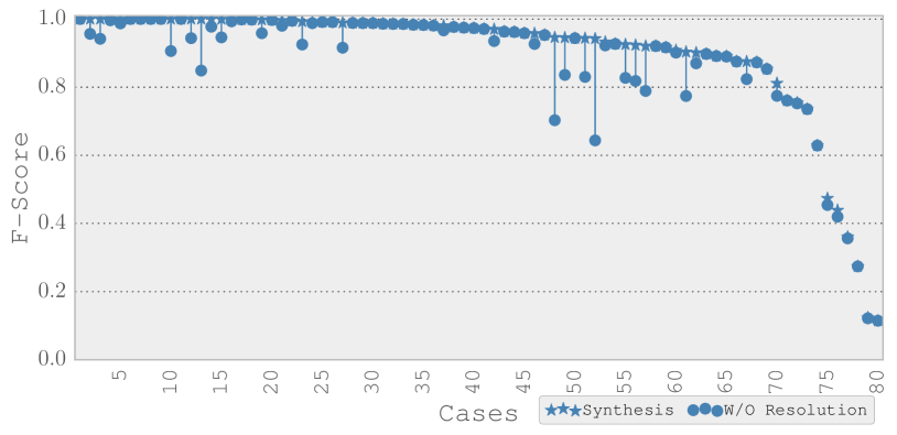
Appendix L Additional Related Work

A related problem is to discover and validate logic rules given knowledge bases [11, 18]. Our problem is not about efficiently discovering rules that are satisfied by a monolithic knowledge base, instead we start from a large set of isolated tables and we synthesize relationships that are functional. To some extent, the relationships discovered by our technique can be used to by humans to complement and enhance existing knowledge bases.

Gupta et al. [20] build Biperpedia, which is an ontology of attributes extracted from query stream and Web text. They focus on attribute name extraction for different entity classes, but not instance values in these relationships.

Mapping tables and FDs are powerful constructs that have been studied in other contexts. For example, authors in [29, 32] study the problem of automatically inferring functional relationships using results extracted by Information-Extraction systems from a text corpus. The difficulty there is that instances extracted for the same relation may be inconsistent. For example, from sentences like “Barack Obama was born in Hawaii” and “Barack Obama was born in USA” IE systems would extract “Barack Obama” on the left, “Hawaii” and “USA” on the right, thus leading to the incorrect conclusion that the relationship of birth-place is not functional. If the results extracted by a text-pattern can be thought of as a table, then the task here is to infer if FD exists for that table, and the challenge is that values in the table may not be consistent. In comparison, we use tables where values are in most cases consistent in the same column. Our task is to go across the boundary of single tables and produce larger relations.

While separate solutions have been proposed for certain applications of mapping tables such as auto-join [24] and auto-fill [4, 38], we argue that there are substantial benefits for using synthesized mapping tables. First, mapping tables are general data assets that can benefit applications beyond auto-join and auto-fill. Synthesizing mapping tables in essence provides a unified approach to these related problems, instead of requiring a different solution for each problem. Second, without mapping tables, techniques like [24] perform heavy duty reasoning at runtime where the complexity grows quickly for large problem instances, and thus have trouble scaling for latency-sensitive scenarios. In comparison, mapping table synthesis happens offline. Applying mapping tables to online applications often reduces to table-lookup that is easy to implement and efficient to scale. Lastly, in trying to productizing auto-join and auto-fill using techniques like [24, 38], we notice that while the quality are good in many cases, they can also be unsatisfactory in others, which prevents wider adoption in commercial systems. Synthesized mapping tables, on the other hand, provide intermediate results that are inspectable, understandable, and verifiable, which are amenable to human curation and continuous user feedback. Thus it is an important problem worth studying.

References

- [1] Google Web Tables. http://research.google.com/tables.
- [2] Microsoft Excel Power Query. http://office.microsoft.com/powerbi.
- [3] Tane: An efficient algorithm for discovering functional and approximate dependencies. In Computer Journal, 1999.
- [4] Z. Abedjan, J. Morcos, M. N. Gubanov, I. F. Ilyas, M. Stonebraker, P. Papotti, and M. Ouzzani. Dataxformer: Leveraging the web for semantic transformations. In CIDR, 2015.
- [5] Y. Bejerano, M. A. Smith, J. Naor, and N. Immorlica. Efficient location area planning for personal communication systems. In Transaction of Networking, 2006.
- [6] P. A. Bernstein, J. Madhavan, and E. Rahm. Generic schema matching, ten years later. In Proceedings of VLDB, 2011.
- [7] K. Bollacker, C. Evans, P. Paritosh, T. Sturge, and J. Taylor. Freebase: A collaboratively created graph database for structuring human knowledge. In SIGMOD, pages 1247–1250, 2008.
- [8] A. Broder. On the resemblance and containment of documents. In SEQUENCES, pages 21–. IEEE Computer Society, 1997.
- [9] M. Bronzi, V. Crescenzi, P. Merialdo, and P. Papotti. Extraction and integration of partially overlapping web sources. PVLDB, pages 805–816, 2013.
- [10] K. Chakrabarti, S. Chaudhuri, Z. Chen, K. Ganjam, and Y. He. Data services leveraging bing’s data assets. IEEE Data Eng. Bull., 2016.
- [11] Y. Chen, S. Goldberg, D. Z. Wang, and S. S. Johri. Ontological pathfinding: Mining first-order knowledge from large knowledge bases. In SIGMOD, 2016.
- [12] F. Chierichetti, N. Dalvi, and R. Kumar. Correlation clustering in mapreduce. In KDD, 2014.
- [13] L. Chitnis, A. Das Sarma, A. Machanavajjhala, and V. Rastogi. Finding connected components in map-reduce in logarithmic rounds. In ICDE, pages 50–61, 2013.
- [14] K. W. Church and P. Hanks. Word association norms, mutual information, and lexicography. Comput. Linguist., 16(1):22–29, 1990.
- [15] E. Cortez, P. A. Bernstein, Y. He, and L. Novik. Annotating database schemas to help enterprise search. Proceedings of VLDB, 2015.
- [16] E. Dahlhaus, D. S. Johnson, C. H. Papadimitriou, P. D. Seymour, and M. Yannakakis. The complexity of multiterminal cuts. SIAM J. Comput., 23(4):864–894, 1994.
- [17] E. D. Demaine, D. Emanuel, A. Fiat, and N. Immorlica. Correlation clustering in general weighted graphs. Theor. Comput. Sci., 361(2):172–187, 2006.
- [18] L. A. Galárraga, C. Teflioudi, K. Hose, and F. Suchanek. Amie: Association rule mining under incomplete evidence in ontological knowledge bases. In WWW, 2013.
- [19] N. Garg, V. V. Vazirani, and M. Yannakakis. Multiway cuts in directed and node weighted graphs. In ICALP, pages 487–498, 1994.
- [20] R. Gupta, A. Halevy, X. Wang, S. E. Whang, and F. Wu. Biperpedia: An ontology for search applications. PVLDB, pages 505–516, 2014.
- [21] B. He and K. C.-C. Chang. Statistical schema matching across web query interfaces. In Proceedings of SIGMOD, 2003.
- [22] H. He, W. Meng, C. Yu, and Z. Wu. Wise-integrator: An automatic integrator of web search interfaces for e-commerce. VLDB Journal, 2004.
- [23] H. He, W. Meng, C. T. Yu, and Z. Wu. Wise-integrator: An automatic integrator of web search interfaces for e-commerce. In PVLDB, 2003.
- [24] Y. He, K. Ganjam, and X. Chu. Sema-join: joining semantically-related tables using big table corpora. In Proceedings of VLDB, 2015.
- [25] J. E. Hopcroft and J. D. Ullman. Set merging algorithms. SIAM Journal on Computing, 2(4):294–303, 1973.
- [26] T. C. Hu. Multi-commodity network flows. Operations Research, 11(3):344–360, 1963.
- [27] R. Kimball and M. Ross. The Data Warehouse Toolkit: The Definitive Guide to Dimensional Modeling. 2002.
- [28] Y. Li, J. Gao, C. Meng, Q. Li, L. Su, B. Zhao, W. Fan, and J. Han. A survey on truth discovery. In SIGKDD Exploration, 2016.
- [29] T. Lin, Mausam, and O. Etzioni. Identifying functional relations in web text. In Proceedings of EMNLP, 2010.
- [30] X. Ling, A. Halevy, F. Wu, and C. Yu. Synthesizing union tables from the web. In IJCAI, pages 2677–2683, 2013.
- [31] E. Rahm and P. A. Bernstein. A survey of approaches to automatic schema matching. The VLDB Journal, 10(4):334–350, Dec. 2001.
- [32] A. Ritter, D. Downey, S. Soderland, and O. Etzioni. It’s a contradiction—no, it’s not: A case study using functional relations. In EMNLP, pages 11–20, 2008.
- [33] W. Su, J. Wang, and F. Lochovsky. Holistic schema matching for web query interfaces. In Proceedings of EDBT, 2006.
- [34] F. M. Suchanek, G. Kasneci, and G. Weikum. Yago: A core of semantic knowledge. In WWW, pages 697–706, 2007.
- [35] E. Ukkonen. Algorithms for approximate string matching. Inf. Control, 64(1-3):100–118, 1985.
- [36] V. Varizani. Approximation algorithms. Springer Verlag, 2001.
- [37] Y. Wang and Y. He. Synthesizing mapping relationships using table corpus. https://www.microsoft.com/en-us/research/wp-content/uploads/2017/03/mapping-synthesis-full.pdf. Technical report.
- [38] M. Yakout, K. Ganjam, K. Chakrabarti, and S. Chaudhuri. Infogather: Entity augmentation and attribute discovery by holistic matching with web tables. In SIGMOD, 2012.
- [39] M. Yannakakis, P. C. Kanellakis, S. S. Cosmadakis, and C. H. Papadimitriou. Cutting and partitioning a graph after a fixed pattern. In J. Diaz, editor, ICALP, pages 712–722, 1983.
- [40] M. Zhang, M. Hadjieleftheriou, B. C. Ooi, C. M. Procopiuc, and D. Srivastava. Automatic discovery of attributes in relational databases. In SIGMOD, pages 109–120, 2011.