Entanglement properties of quantum grid states

Abstract

Grid states form a discrete set of mixed quantum states that can be described by graphs. We characterize the entanglement properties of these states and provide methods to evaluate entanglement criteria for grid states in a graphical way. With these ideas we find bound entangled grid states for two-particle systems of any dimension and multiparticle grid states that provide examples for the different aspects of genuine multiparticle entanglement. Our findings suggest that entanglement theory for grid states, although being a discrete set, has already a complexity similar to the one for general states.

I Introduction

Entanglement is a fundamental phenomenon of quantum theory bell ; werner and is the key to the successes in the steadily maturing field of quantum technologies metrology ; msmtbased . A rich mathematical theory of entanglement has been developed in recent years horodecki , with one of its main aims to devise techniques to detect and quantify the entanglement present in a physical system. This direction has seen some success, with a number of results being applied in a laboratory setting detecting . In general however, testing if a density matrix describes a state that is entangled or separable is highly non-trivial: so far, no necessary and sufficient criterion for separability has been discovered that is efficiently computable. In a perhaps discouraging development, the problem of deciding if an arbitrary density matrix is separable turns out to be NP-hard gurvits ; sevag ; ioannou , suggesting that an efficient “silver bullet” entanglement criterion is permanently out of reach.

In this work we propose the study of a simple family of quantum states called grid states as a toy model for mixed state entanglement. Grid states are represented using a combinatorial object called a grid-labelled graph combent , and their entanglement properties can be determined by considering the structure of this graph. We show that despite their deceptively simple definition, grid states can exhibit a rich variety of entanglement properties. In particular, we demonstrate that there are bipartite bound entangled grid states in all dimensions. We also extend the grid state framework to multiparticle states, explicitly constructing a $3\times 3\times 3$ grid state that is positive under partial transpose (PPT) over all bipartitions, but is genuinely multipartite entangled. This provides an example of a state which cannot be characterized by the method of PPT mixtures pptmixer , which is the strongest criterion for multiparticle entanglement so far.

Note that the fact that many NP-complete problems are about graphs gj gives further motivation for the study of grid states: it may be possible to prove that determining separability of grid states is NP-hard by reduction from a graph problem, e.g., SubgraphIsomorphism. Such a result would imply the known NP-hardness result for the more general problem. A proof of NP-hardness for these states would strengthen the complexity lower bound for the separability problem in its full generality. The fact that we are able to demonstrate non-trivial entanglement structure in grid states gives weight to the idea that this problem is computationally intractable. In this way, our approach also initiates a new strategy in studying entanglement. So far, many works have been concerned with the study of certain families of quantum states (e.g., with symmetries), where the separability problem is simplified or can be solved werner ; sym1 ; sym2 ; sym3 . Contrary to that, our strategy is to identify a small and discrete family of states, for which the separability problem has a similar complexity as in the general case. We believe that this can be a way to shed new light on open problems in quantum information theory. We add that recently the separability problem for so-called Dicke-diagonal states has been shown to be NP-hard yu ; tura , but this is a continuous family of states. Moreover, due to the high symmetry, not all possible types of entanglement are present in this type of states, e.g, a multiparticle state that is separable for one bipartition is already fully separable eckert ; ichikawa .

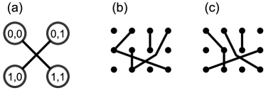
Figure 1: (a): A simple example of a grid-labelled graph. The depicted graph corresponds to the uniform mixture of two Bell states $\rho=\frac{1}{4}(|00\rangle-|11\rangle)(\langle 00|-\langle 11|)+\frac{1}{4}(|01\rangle-|10\rangle)(\langle 01|-\langle 10|)$. (b) and (c): Example of the action of a partial transposition. The graph in (b) represents a $3\times 4$ state, and the graph in (c) is used for determining the partial transposition. One sees that the degree of the vertex $(1,0)$ changes, hence the state in NPT and entangled. See the text for further details.

II Grid states

We say that a quantum state is an $m\times n$ grid state if it is the uniform mixture of pure states of the form $(|ij\rangle-|kl\rangle)/\sqrt{2}$, with $0\leq i,k<m$ and $0\leq j,l<n$. Such a mixed state can be represented on a graph with $mn$ vertices arranged in an $m\times n$ grid by associating each state $|ij\rangle-|kl\rangle/\sqrt{2}$ with an edge between vertices $(i,j)$ and $(k,l)$. We call such a graph a grid-labelled graph for the implicit Cartesian labelling of the vertices. For example, Fig. 1 shows a grid-labelled graph that corresponds to the uniform mixture over the Bell states $|\Psi^{-}\rangle$ and $|\Phi^{-}\rangle$. In general, if $G$ is a grid-labelled graph, we denote its corresponding grid state density matrix by $\rho(G)$. It is straightforward to see that two different grid-labelled graphs lead to two different quantum states. When context allows, we refer to grid-labelled graphs simply as graphs.

In Ref. combent it is shown that for any grid-labelled graph $G$, the density matrix $\rho(G)$ corresponds to the Laplacian matrix of $G$, normalised to have trace $1$. The Laplacian matrix of a graph with $k$ vertices is an $k\times k$ matrix $L(G)$ where each diagonal entry $[L(G)]_{ii}$ is equal to the degree of vertex $i$; each off diagonal entry $[L(G)]_{ij}$ is $-1$ if there is an edge between vertices $i$ and $j$, and $0$ otherwise.

Considering the Laplacian matrix of a graph as the density matrix of a quantum state is an approach initiated by Braunstein et al. braunstein1 , and further developed in Refs. braunstein2 ; hildebrand ; wu , where it is shown that entanglement properties of the state are manifested in the structure of the corresponding graph. A drawback of the original approach is that the entanglement properties of the state change when the vertices are labelled in a different way. The study of grid-labelled graphs by the authors in Ref. combent remedies this issue by imposing the Cartesian vertex labelling. We also add that mixtures of Bell-type states were used in Ref. piani to construct bound entangled states, but this employed a different strategy.

The fact that the density matrix of a grid state corresponds to the Laplacian of the corresponding graph means that a number of results from the already established literature on graph Laplacian states can be brought to bear on grid states. In particular, the entanglement criterion of the positivity of the partial transpose (PPT) peres ; horodeckisep can be formulated in terms of grid states. For a given graph $G$, positivity of $\rho(G)^{T_{B}}$ can be determined by considering another graph $G^{\Gamma}$. This is constructed from $G$ by flipping the edges in each rectangle: an edge $\{(i,j),(k,l)\}$ belongs to $G^{\Gamma}$ if and only if $\{(i,l),(k,j)\}$ belongs to $G$ (see Fig. 1 for an example).

By definition, separable states are of the form

$$\rho_{AB}=\sum_{k}p_{k}\rho^{(k)}_{A}\otimes\rho^{(k)}_{B},$$ (1)

where the $p_{k}$ form a probability distribution, and if a state is not separable then it is entangled. The PPT criterion states that for a separable state the partial transposition has no negative eigenvalues, $\rho(G)^{T_{B}}\geq 0$. For grid states, it can be shown that $\rho(G)$ is PPT iff the degree of $(i,j)$ in $G$ is equal to the degree of $(i,j)$ in $G^{\Gamma}$, for all vertices $(i,j)$ combent . Hence, if taking the partial transpose of $G$ does not preserve the degrees of the vertices then $\rho(G)$ is entangled. Naturally, this “degree criterion” is necessary and sufficient for separability in $2\times 2$ and $2\times 3$ grid states. Remarkably, it is also necessary and sufficient for graph Laplacian states in $\mathbb{C}^{2}\otimes\mathbb{C}^{q}$ wu , and so this is also the case for $2\times q$ grid states. It is easily verified that the grid states illustrated in Fig. 1 (a) and in Fig. 2 (a) satisfy the degree criterion and are therefore positive under partial transpose (PPT). However, it can be verified by the computable cross norm or realignment criterion rudolph ; mr that the state in Fig. 2 (a) is entangled. Such a state, constructed in Ref. hildebrand and referred to as a cross-hatch state in combent is therefore bound entangled. Bound entangled states are at the heart of many problems in quantum information theory be1 ; be2 , therefore it is highly desirable to identify such states in the bipartite or multipartite setting.

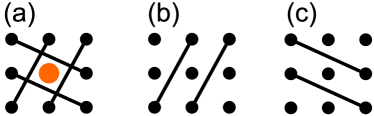
Figure 2: Graph (a) is the cross-hatch graph. Graph (b) is obtained by performing row surgery on the marked vertex of (a), and graph (c) in the same way but by column surgery. See the text for further details.

III The range criterion and graph surgery

Our main tool for showing that grid states have a rich entanglement structure is a graphical way to evaluate the range criterion range . This criterion is one of the main criteria to detect bound entanglement in the bipartite and multipartite setting. The criterion is stated like so: if a bipartite density operator $\rho_{AB}$ is separable then there exists a set of product vectors $P=\{|a_{1}\rangle|b_{1}\rangle,\dots,|a_{r}\rangle|b_{r}\rangle\}$ such that $P$ spans the range of $\rho_{AB}$ and, at the same time, $\{|a_{1}\rangle|b_{1}^{*}\rangle,\dots,|a_{r}\rangle|b_{r}^{*}\rangle\}$ spans the range of $\rho_{AB}^{T_{B}}$. Note, however, that it is in general very difficult to determine all sets of product vectors that span a given subspace. The range criterion can be immediately generalised to the multipartite case horodecki .

We use the following corollary: if a rank $r$ density operator has less than $r$ product vectors in its range then it is entangled. In order to utilize this, we demonstrate a technique we call graph surgery as a way of determining properties of the range of a grid state. The surgery procedure removes edges from a grid-labelled graph, and it can be shown that the graph that results has the same number of product vectors in its range as the original graph. Surgery can be applied repeatedly, often producing grid states whose ranges are easily determined.

In particular, let $G$ be a graph with an isolated vertex $(i,j)$, meaning that this vertex has no neighbours and so degree $0$. Then we obtain another graph $G_{(i,j)}^{R}$ by performing the procedure row surgery on the isolated vertex. This consists of two steps:

Row Surgery:
(1) CUT: Remove all edges attached to vertices in row $i$.
(2) STITCH: For every pair of vertices not on row $i$: if there was a path between them that has been destroyed by the CUT step, then add an edge between them.

Note that the STITCH step is not unique: any edge can be added, provided it reconnects the components that have been disconnected. As we shall see later, it does not matter which edge (or edges) are added. In the same way, we can define column surgery, which produces $G_{(i,j)}^{C}$ in an analogous manner but acting on column $j$. Examples of these operations are shown in Figs. 2 and 3. In Fig. 2 we demonstrate the result of performing row surgery (b) and column surgery (c) on vertex $(1,1)$ of graph (a). Since the CUT step does not disconnect any connected components of the graph in this case, the STITCH step is not required. In Fig. 3 we demonstrate a more complicated example of surgery. The row surgery on vertex $(1,4)$ removes the pre-existing path between vertices $(0,4)$ and $(3,1)$. This can be rectified by adding an edge between $(3,1)$ and $(0,4)$.

Our results follow from the following observation, which is formalised and proved in the Appendix.

Observation 1. Any product vector $|\alpha\rangle|\beta\rangle$ in the range of $\rho(G)$ must be in the range of $\rho(G_{(i,j)}^{R})$ or the range of $\rho(G_{(i,j)}^{C})$, for any isolated vertex $(i,j)$ of $G$.

This means that we can iterate row surgery and column surgery and simplify the graph, this can easily be done with the help of a computer mathematica . During this iteration, it is clear that not all isolated vertices yield new information about the range of a grid state when surgery is performed. Consider a row $i$ where every vertex is isolated [e.g., the second row in Fig. 2(b)]. Then, performing row surgery on any vertex $(i,j)$ [e.g., on vertex (1,0) in Fig. 2(b)] on that row has no effect and we obtain the trivial statement that a product vector in the range of $\rho(G)$ is in the range of $\rho(G)$ or $\rho(G^{C}_{(i,j)})$. This is also the case for isolated vertices on an isolated column.

So, one should focus on isolated vertices which give new information and we therefore call isolated vertices that are on a non-isolated row and column viable [e.g., vertex (0,0) in Fig. 2(b)]. Starting from a viable vertex, surgeries can be iterated until there are no longer any viable vertices in the graph, at which point the range of the graph can sometimes be easily determined.

IV Bipartite entanglement

Now we demonstrate how the surgery procedure can be applied in conjunction with Observation 1 to determine families of bipartite bound entangled states. We first demonstrate that the grid state corresponding to the cross-hatch graph in Fig. 2(a) is entangled. The isolated vertex in the middle is viable. Applying row surgery on this middle vertex yields graph (b), while column surgery gives graph (c). Due to the rotational symmetry, we consider only the former, which has two viable vertices, $(0,0)$ and $(2,2)$. Starting with $(0,0)$, row surgery eliminates both edges giving the empty graph, and column surgery eliminates one, leaving the graph with a single diagonal edge. Another surgery can eliminate this edge, giving the empty graph. It is clear that any sequence of surgeries starting at $(2,2)$ has a similar outcome. So, all sequences of surgeries will terminate in the empty graph. Observation 1 tells us that any product vector in the range of $\rho(G)$ must be in the range of one of these empty graphs, which is not possible because they have zero-dimensional ranges. So, there are no product vectors in the range and the state $\rho(G)$ is entangled. Since it is PPT, it is bound entangled.

The cross-hatch structure of the graph can be generalised to arbitrary grid sizes. It is easily checked that these graphs all are PPT. It is clear from similar reasoning to the $3\times 3$ case that for all grid sizes all sequences of surgeries terminate with empty graphs: every subgraph of a cross-hatch graph has at least one viable vertex. So all cross-hatch graphs correspond to bound entangled states.

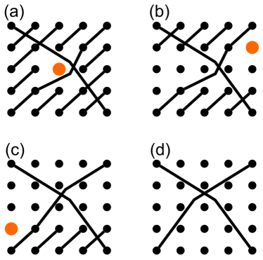
Figure 3: A sequence of row surgeries being performed on the square-loop graph. Target vertices are highlighted in orange: for example, (b) is obtained by performing row surgery on isolated vertex $(2,2)$ of graph (a), and so on. Note that graphs (c) and (d) require the STITCH step to be performed, with edges $\{(0,4),(3,1)\}$ and $\{(0,4),(4,0)\}$ added respectively.

The second bipartite example is the square-loop graph $G$, see Fig. 3(a). Performing row surgery on the viable isolated vertex $(2,2)$ gives us graph (b), which has two viable isolated vertices: $(1,4)$ and $(4,1)$. Row surgery on $(1,4)$ yields graph (c). We ask the reader to verify that the surgeries can be iterated in a similar way, and that any sequence of surgeries leads to one of two graphs: the $5\times 5$ empty graph, or the ‘X’-shaped graph (d). Since the graph $G$ has $25$ vertices and $11$ connected components, the grid state is of rank $25-11=14$, see Lemma 2 in the Appendix. If $\rho(G)$ were separable then its range must have a product basis. But the ‘X’-shaped grid state has rank $25-23=2$ and the empty graph is of rank zero. So, these graphs do not contain enough product vectors.

Finally, note that the cross-hatch states are edge states edgestates , as there are no product vectors in their range. Edge states are highly entangled bound entangled states, lying at the border between PPT and NPT states. Further, all grid states are Schmidt rank two: by definition they are equal to uniform mixtures of pure states of the form $(|ij\rangle-|kl\rangle)/\sqrt{2}$.

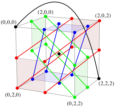
Figure 4: The three-partite cross-hatch graph on a $3\times 3\times 3$ grid. This corresponds to a permutationally invariant rank 13 state in a three-qutrit system. The state is PPT for any bipartition, nevertheless it is genuine multiparticle entangled. The coulours of the edges and the squares are introduced to guide the eye.

V Multiparticle entanglement

Interestingly, the constructions can be generalized to the multiparticle case, yielding further examples of quantum states with surprising entanglement properties. Let us consider graphs on an $l\times m\times n$ grid, which correspond to tripartite grid states $\rho_{ABC}\in\mathbb{C}^{l}\otimes\mathbb{C}^{m}\otimes\mathbb{C}^{n}$. The cross-hatch construction can be generalised to the $3\times 3\times 3$ grid, which is illustrated in Fig. 4. Analoguous the bipartite case, a link between two vertices $ijk$ and $rst$ corresponds to the state $(|ijk\rangle-|rst\rangle)/\sqrt{2}.$

First, one can see by direct inspection that the graph has a symmetry, leading to a permutationally invariant state. Then, one can directly check that the state is PPT for any of the possible bipartitions $A|BC$, $B|AC$, and $C|AB$. In addition, one can apply the iteration of surgeries for the bipartitions. After nine iterations, one arrives at an empty graph, proving that there are no product vectors of the type $|\phi\rangle_{A}\otimes|\psi\rangle_{BC}$ (or similar vectors for other bipartitions) in the range of $\rho(G)$ mathematica . This implies that the state is genuine multiparticle entangled detecting . So, this state is an example where the entanglement criterion of PPT mixtures fails pptmixer . This criterion is the strongest criterion for multiparticle entanglement, and so far only three examples of states are known which cannot be detected by it pianimora ; hubersengupta ; korea . This demonstrates that also weak and rare forms of multiparticle entanglement can be found among grid states.

It is clear how to generalise this cross-hatch structure to the $l\times l\times l$ case. Indeed, it seems likely that such states exist in the $N$-partite case, and can be constructed by connecting faces of the $N$-dimensional hypercube.

VI Conclusion

We have shown that grid states can be highly non-trivial entangled states. Based on graphical ways to evaluate the PPT criterion and the range criterion, we have demonstrated that for all bipartite dimensions there exists bound entangled grid states. We have generalized grid states to the multiparticle case, and again is turned out that these states can have complicated entanglement properties. This makes grid states a valuable test-bed for various entanglement criteria.

The diversity of the states we can generate with this formalism can be interpreted to mean that testing separability of even this restricted class of states may be NP-hard. Furthermore, perhaps a graph theoretic reduction could be used in a hardness proof, potentially simplifying the argument of Gurvits gurvits . On the other hand, the elegance of the graphical description makes the formalism an attractive tool for the study of quantum entanglement and the interplay between different entanglement criteria.

For further work, it would be highly desirable to derive algorithms to prove separability of grid states in a graphical language. This is needed to analyze the algorithmic complexity of the separability problem for grid states further. Second, it would be useful if one can identify graphical transformations that keep the entanglement properties invariant, as they induce only local unitary transformations of the state. Similar rules are known for the families of cluster states and graph states hein ; tsimakuridze . Finally, natural generalisations of the grid state concept would include hypergraphs and weighted graphs.

We thank Felix Huber and Danial Dervovic for helpful discussions. This work has been supported by the UK EPSRC (EP/L015242/1), the ERC (Consolidator Grant 683107/TempoQ), and the DFG. JL thanks the Theoretical Quantum Optics group at Universität Siegen for their hospitality.

VII Appendix

Our results follow by application of Observation 1, which we prove here. We first restate it in a more formal manner. In what follows, we denote the kernel and range of a density operator $\rho$ by $K(\rho)$ and $R(\rho)$ respectively.

Observation 1’. Let $G$ be a grid-labelled graph with isolated vertex $(i,j)\in V(G)$. For all product vectors $|\alpha\rangle|\beta\rangle\in\mathbb{C}^{m}\otimes\mathbb{C}^{n}$, if $|\alpha\rangle|\beta\rangle\in R[\rho(G)]$ then $|\alpha\rangle|\beta\rangle\in R[\rho(G_{(i,j)}^{R})]$ or $|\alpha\rangle|\beta\rangle\in R[\rho(G_{(i,j)}^{C})]$.

Before proving this result, we need two lemmata. The following lemma provides a characterization of the range of a grid state. For its formulation, we denote by $C(G)$ the set of connected components of a graph. Here, also disconnected vertices are considered to constitute a connected component. For example, the cross hatch graph in Fig. 2(a) in the main text has five connected components, $|C(G)|=5.$ We also associate with every grid-labelled graph $G$ the state $|G\rangle=\sum_{(i,j)\in V^{{}^{\prime}}(G)}|ij\rangle$, where $V^{{}^{\prime}}(G)=\{(i,j)\in V(G)~{}:~{}d[(i,j)]>0\}$ is the set of vertices of $G$ with non-zero degree. This construction can also be applied to a single connected component $S\in C(G).$

Lemma 2. Let $G$ be an $m\times n$ grid-labelled graph, and let $C(G)$ denote the set of its connected components. Then $|\psi\rangle\in R(\rho(G))$ if and only if $|\psi\rangle\perp|S\rangle$ for all $S\in C(G)$. This implies that for any $m\times n$ vertex grid-labelled graph $G$, the dimension of the kernel of $\rho(G)$ is equal to the number of connected components $|C(G)|$. Therefore, the rank of $\rho(G)$ is equal to $m\times n-|C(G)|$.

Proof of Lemma 2. For all graphs $G$, $\rho(G)$ is Hermitean so $|\psi\rangle\in R(\rho(G))$ if and only if $|\psi\rangle\perp K[\rho(G)]$.

For any connected component $S\in C(G)$ with $k$ vertices, $\rho(S)|S\rangle=0$, so $|S\rangle\in K[\rho(S)]$. Since $S$ is connected, it has a spanning tree $T$ with $k-1$ edges. The edges of $T$ correspond to a set of linearly independent vectors $(|ij\rangle-|kl\rangle)/\sqrt{2}$ in the range of $R[\rho(S)]$, so $\text{dim}(K[\rho(S)])\leq k-(k-1)=1$. Therefore, $K[\rho(S)]=\text{span}_{\mathbb{C}}(|S\rangle)$.

The density operator $\rho(G)$ can be decomposed in terms of $C(G)$,

$$\rho(G) =\frac{1}{2|E|}\sum_{\{(i,j),(k,l)\}\in E(G)}(|ij\rangle-|kl\rangle)(\langle ij|-\langle kl|)$$

$$=\frac{1}{2|E|}\sum_{S\in C(G)}2|E(S)|\rho(S)$$

$$=\sum_{S\in C(G)}\frac{|E(S)|}{|E(G)|}\rho(S).$$ (2)

By definition the components $S$ have no edges in common, so $|\psi\rangle\perp K[\rho(G)]$ if and only if $|\psi\rangle\perp K[\rho(S)]=\text{span}_{\mathbb{C}}(|S\rangle)$ for all $S\in C(G)$. $\hfill\Box$

To proceed we will need to define the vectors

$$|G_{i,*}\rangle=\sum_{\begin{subarray}{c}(k,l)\in V(G)\\ k\neq i\end{subarray}}|kl\rangle$$ (3)

and

$$|G_{*,j}\rangle=\sum_{\begin{subarray}{c}(k,l)\in V(G)\\ l\neq j\end{subarray}}|kl\rangle.$$ (4)

for any subgraph $G$ of a grid-labelled graph. Then we have:

Lemma 3. Let $G$ be a grid-labelled graph with $m\times n$ vertices. If a state $|\psi\rangle$ is orthogonal to all states in

• $\{|S_{i,*}\rangle~{}:~{}S\in C(G)\}$ and $\{|i,1\rangle,\dots,|i,n\rangle\}$ then $|\psi\rangle\in R[\rho(G_{(i,j)}^{R})]$;

• $\{|S_{*,j}\rangle~{}:~{}S\in C(G)\}$ and $\{|1,j\rangle,\dots,|m,j\rangle\}$ then $|\psi\rangle\in R[\rho(G_{(i,j)}^{C})]$.

Proof of Lemma 3. It is clear that $G_{(i,j)}^{R}$ can be obtained by considering the effect of surgery on each connected component of $G$ separately. For such a component $S\in C(G)$, we have that $K[\rho(S)]=\sum_{(k,l)\in V(S)}|kl\rangle$. Performing the CUT step of surgery on row $i$ of $S$ removes all edges to vertices in that row, which introduces new isolated vertices. The STITCH step then ensures that the remnants of the graph remain connected. Therefore, if a state $|\psi\rangle$ is orthogonal to $\sum_{(k,l)\in V(S)}|kl\rangle$ for $k\neq i$, and is orthogonal to $\{|i,q\rangle\}$ for all of the new isolated vertices $(i,q)$, then it is in the range of $\rho(S_{(i,j)}^{R})$ by Lemma 2. It is clear that if $|\psi\rangle$ is orthogonal to each of the states $|S_{i,*}\rangle$ for $S\in C(G)$, as well as all the isolated vertex states $|i,1\rangle,\dots,|i,m\rangle$ introduced by performing CUT on each component then it is in the range of $\rho(G_{(i,j)}^{R})$ by Lemma 2. By similar reasoning, the same is true for the graph obtained by column surgery. $\sqcap$$\sqcup$

We may now prove the Observation.

Proof of Observation 1’. Since $(i,j)$ is isolated then $|i,j\rangle\in K[\rho(G)]$. Therefore, if $|\alpha\rangle|\beta\rangle\in R(\rho(G))$ then either $|\alpha\rangle\perp|i\rangle$ or $|\beta\rangle\perp|j\rangle$. Suppose the former is the case. Then clearly $|\alpha\rangle|\beta\rangle$ is orthogonal to all $|i,1\rangle,\dots,|i,m\rangle$. Further, we know that for all $S\in C(G)$, $|\alpha\rangle|\beta\rangle$ is orthogonal to $|S\rangle$, and so must be orthogonal to $|S_{i,*}\rangle$. Therefore, by Lemma 3 it must be in the range of $\rho(G_{(i,j)}^{R})$. If we instead assume that $|\beta\rangle\perp|j\rangle$ then by similar reasoning, $|\alpha\rangle|\beta\rangle\in R[\rho(G_{(i,j)}^{C})]$. $\sqcap$$\sqcup$

References

- (1) J. S. Bell, Physics 1, 3, 195 (1964).
- (2) R. F. Werner, Phys. Rev. A 40, 4277 (1989).
- (3) V. Giovannetti, S. Lloyd, and L. Maccone, Nat. Photon. 5, 222 (2011).
- (4) H. J. Briegel, D. E. Browne, W. Dür, R. Raussendorf, and M. Van den Nest, Nat. Phys. 5, 19 (2009).
- (5) R. Horodecki, P. Horodecki, M. Horodecki, and K. Horodecki, Rev. Mod. Phys. 81, 865 (2009).
- (6) O. Gühne and G. Tóth, Phys. Rep. 474, 1 (2009).
- (7) L. Gurvits, Proc. of the 35th ACM Symp. on Theory of Comp. (STOC), pp. 10-19, (2003).
- (8) S. Gharibian, Quantum Inf. Comput. 10, 343 (2010).
- (9) L. M. Ioannou, Quantum Inf. Comput. 7, 4 (2007).
- (10) J. Lockhart and S. Severini, arXiv:1605.03564.
- (11) B. Jungnitsch, T. Moroder, and O. Gühne, Phys. Rev. Lett. 106, 190502 (2011).
- (12) M. R. Garey and D. S. Johnson, “Computers and Intractability: A Guide to the Theory of NP-Completeness”, W. H. Freeman & Co. New York, NY, USA (1979).
- (13) K. G. H. Vollbrecht and R. F. Werner, Phys. Rev. A 64, 062307 (2001).
- (14) C. Eltschka and J. Siewert, Phys. Rev. Lett. 108, 020502 (2012).
- (15) L.E. Buchholz, T. Moroder, and O. Gühne, Ann. Phys. (Berlin) 528, 278 (2016).
- (16) N. Yu, Phys. Rev. A 94, 060101(R) (2016).
- (17) J. Tura, A. Aloy, R. Quesada, M. Lewenstein, and A. Sanpera, Quantum 2, 45 (2018).
- (18) K. Eckert, J. Schliemann, D. Bruß, and M. Lewenstein, Ann. Phys. (New York) 299, 88 (2002).
- (19) T. Ichikawa, T. Sasaki, I. Tsutsui, and N. Yonezawa, Phys. Rev. A 78, 052105 (2008).
- (20) S. L. Braunstein, S. Ghosh, and S. Severini, Ann. Comb. 10, 291 (2006).
- (21) S. L. Braunstein, S. Ghosh, T. Mansour, S. Severini, and R. C. Wilson, Phys. Rev. A 73, 012320 (2006).
- (22) R. Hildebrand, S. Mancini, and S. Severini, Math. Struct. in Comp. Science 8, 205 (2008).
- (23) C. W. Wu, Phys. Lett. A 351, 18 (2006).
- (24) M. Piani, Phys. Rev. A 73, 012345 (2006).
- (25) A. Peres, Phys. Rev. Lett. 77, 1413 (1996).
- (26) M. Horodecki, P. Horodecki, and R. Horodecki, Phys. Lett. A 223, 1 (1996).
- (27) O. Rudolph, Quantum Inf. Process. 4, 219 (2005).
- (28) K. Chen, L. Wu, Quantum Inf. Comput. 3, 193 (2003).
- (29) K. Horodecki, M. Horodecki, P. Horodecki, and J. Oppenheim, Phys. Rev. Lett. 94, 160502 (2005).
- (30) A. Acín, J. I. Cirac, and Ll. Masanes, Phys. Rev. Lett. 92, 107903 (2004).
- (31) P. Horodecki, Phys. Lett. A 232, 333 (1997).
- (32) A Mathematica file for performing iterations of surgery operations is available upon request.
- (33) M. Lewenstein, B. Kraus, J. I. Cirac, and P. Horodecki, Phys. Rev. A 62, 052310 (2000).
- (34) M. Piani and C. Mora, Phys. Rev. A 75, 012305 (2007).
- (35) M. Huber and R. Sengupta, Phys. Rev. Lett. 113, 100501 (2014).
- (36) K.-C. Ha and S.-H. Kye, Phys. Rev. A 93, 032315 (2016).
- (37) M. Hein, J. Eisert, and H.J. Briegel, Phys. Rev. A 69, 062311 (2004).
- (38) N. Tsimakuridze and O. Gühne, J. Phys. A: Math. Theor. 50, 195302 (2017).