GSplit LBI: Taming the Procedural Bias in Neuroimaging for Disease Prediction

Abstract

In voxel-based neuroimage analysis, lesion features have been the main focus in disease prediction due to their interpretability with respect to the related diseases. However, we observe that there exist another type of features introduced during the preprocessing steps and we call them “Procedural Bias”. Besides, such bias can be leveraged to improve classification accuracy. Nevertheless, most existing models suffer from either under-fit without considering procedural bias or poor interpretability without differentiating such bias from lesion ones. In this paper, a novel dual-task algorithm namely GSplit LBI is proposed to resolve this problem. By introducing an augmented variable enforced to be structural sparsity with a variable splitting term, the estimators for prediction and selecting lesion features can be optimized separately and mutually monitored by each other following an iterative scheme. Empirical experiments have been evaluated on the Alzheimer’s Disease Neuroimaging Initiative (ADNI) database. The advantage of proposed model is verified by improved stability of selected lesion features and better classification results.

1 Introduction

Usually, the first step of voxel-based neuroimage analysis requires preprocessing the T₁-weighted image, such as segmentation and registration of grey matter (GM), white matter (WM) and cerebral spinal fluid (CSF). However, some systematic biases due to scanner difference and different population etc., can be introduced in this pipeline [2]. Part of them can be helpful to the discrimination of subjects from normal controls (NC), but may not be directly related to the disease. For example in structural Magnetic Resonance Imaging (sMRI) images of subjects with Alzheimer’s Disease (AD), after spatial normalization during simultaneous registration of GM, WM and CSF, the GM voxels surrounding lateral ventricle and subarachnoid space etc. may be mistakenly enlarged caused by the enlargement of CSF space in those locations [2] compared to normal template, as shown in Fig. 1. Although these voxels/features are highly correlated with disease, they can’t be regarded as lesion features in an interpretable model. In this paper we refer to them as “Procedural Bias”, which should be identified but is neglected in the literature. We observe that it can be harnessed in our voxel-based image analysis to improve the prediction of disease.

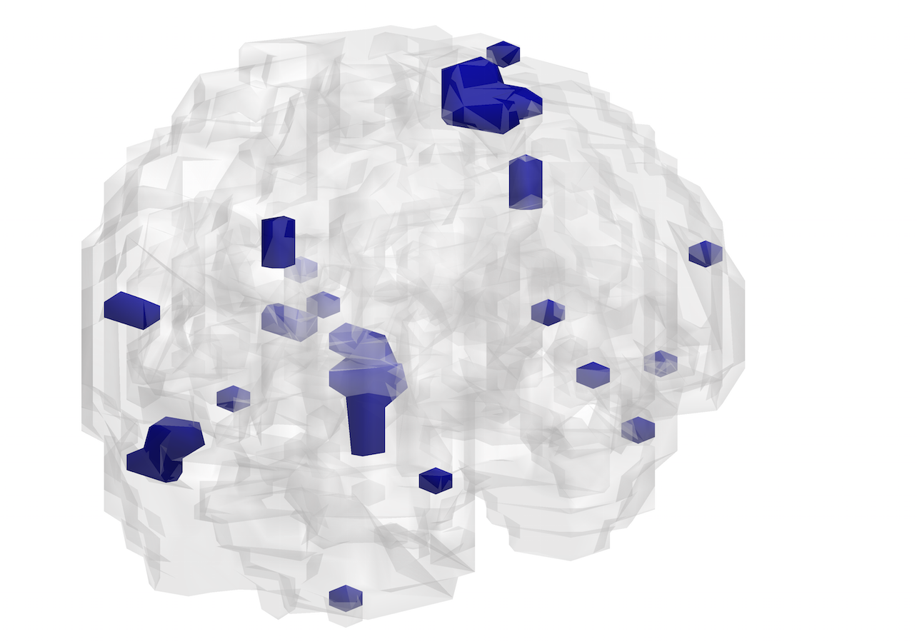
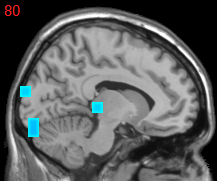
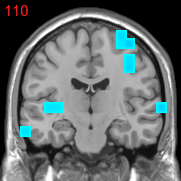
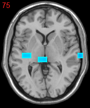
Figure 1: The overlapped voxels among top 150 negative value voxels in each fold of $\beta_{pre}$ at the time corresponding to the best average prediction result in the path of GSplit LBI using 10-fold cross-validation. For subjects with AD, they represent enlarged GM voxels surrounding lateral ventricle, subarachnoid space, edge of gyrus, etc.

Together with procedural bias, the lesion features are vital for prediction and lesion regions analysis tasks, which are commonly solved by two types of regularization models. Specifically, one kind of models such as general losses with $l_{2}$ penalty, elastic net [15] and graphnet [5] select strongly correlated features to minimize classification error. However, such models don’t differentiate features either introduced by disease or procedural bias and may also introduce redundant features. Hence, the interpretability of such models are poor and the models are prone to over-fit. The other kind of models with sparsity enforcement such as TV-$L_{1}$ (Combination of Total Variation [9] and $L_{1}$) and particularly $n^{2}$ GFL [13] enforce strong prior of disease on the parameters of the models introduced in order to capture the lesion features. Although such features are disease-relevant and the selection is stable, the models ignore the inevitable procedural bias, hence, they are losing some prediction power.

To incorporate both tasks of prediction and selection of lesion features, we propose an iterative dual-task algorithm namely Generalized Split LBI (GSplit LBI) which can have better model selection consistency than generalized lasso [11]. Specifically, by the introduction of variable splitting term inspired by Split LBI [6], two estimators are introduced and split apart. One estimator is for prediction and the other is for selecting lesion features, both of which can be pursued separately with a gap control. Following an iterative scheme, they will be mutually monitored by each other: the estimator for selecting lesion features is gradually monitored to pursue stable lesion features; on the other hand, the estimator for prediction is also monitored to exploit both the procedural bias and lesion features to improve prediction. To show the validity of the proposed method, we successfully apply our model to voxel-based sMRI analysis for AD, which is challenging and attracts increasing attention.

2 Method

2.1 GSplit LBI Algorithm

Our dataset consists of $N$ samples $\{x_{i},y_{i}\}_{1}^{N}$ where $x_{i}\in\mathbb{R}^{p}$ collects the $i^{th}$ neuroimaging data with $p$ voxels and $y_{i}=\{\pm 1\}$ indicates the disease status ($-1$ for Alzheimer’s disease in this paper). $X\in\mathbb{R}^{N\times p}$ and $y\in\mathbb{R}^{p}$ are concatenations of $\{x_{i}\}_{i}$ and $\{y_{i}\}_{i}$. Consider a general linear model to predict the disease status (with the intercept parameter $\beta_{0}\in\mathbb{R}$),

$$\log P(y_{i}=1|x_{i})-\log P(y_{i}=-1|x_{i})=x_{i}^{T}\beta_{pre}+\beta_{0}.$$ (2.1)

A desired estimator $\beta_{pre}\in\mathbb{R}^{p}$ should not only fit the data by maximizing the log-likelihood in logistic regression, but also satisfy the following types of structural sparsity: (1) the number of voxels involved in the disease prediction is small, so $\beta_{pre}$ is sparse; (2) the voxel activities should be geometrically clustered or 3D-smooth, suggesting a TV-type sparsity on $D_{G}\beta_{pre}$ where $D_{G}$ is a graph difference operator; (3) the degenerate GM voxels in AD are captured by nonnegative component in $\beta_{pre}$. However, the existing procedural bias may violate these a priori sparsity properties, esp. the third one, yet increase the prediction power.

To overcome this issue, we adopt a variable splitting idea in [6] by introducing an auxiliary variable $\gamma\in\mathbb{R}^{|V|+|E|}$ to achieve these sparsity requirements separately, while controlling the gap from $D\beta_{pre}$ with penalty $S_{\rho}(\beta_{pre},\gamma):=\|D\beta_{pre}-\gamma\|_{2}^{2}:=\|\beta_{pre}-\gamma_{V}\|_{2}^{2}+\|\rho D_{G}\beta_{pre}-\gamma_{G}\|_{2}^{2}$ with $\displaystyle\gamma=\left[\begin{array}[]{cc}\gamma_{V}^{T}&\gamma_{G}^{T}\end{array}\right]^{T}$ and $\displaystyle D=\left[\begin{array}[]{cc}I&\rho D_{G}^{T}\end{array}\right]^{T}$. Here $\rho$ controls the trade-off between different types of sparsity. Our purpose is thus of two-folds: (1) use $\beta_{pre}$ for prediction; (2) enforce sparsity on $\gamma$. Such a dual-task scheme can be illustrated by Fig. 6.

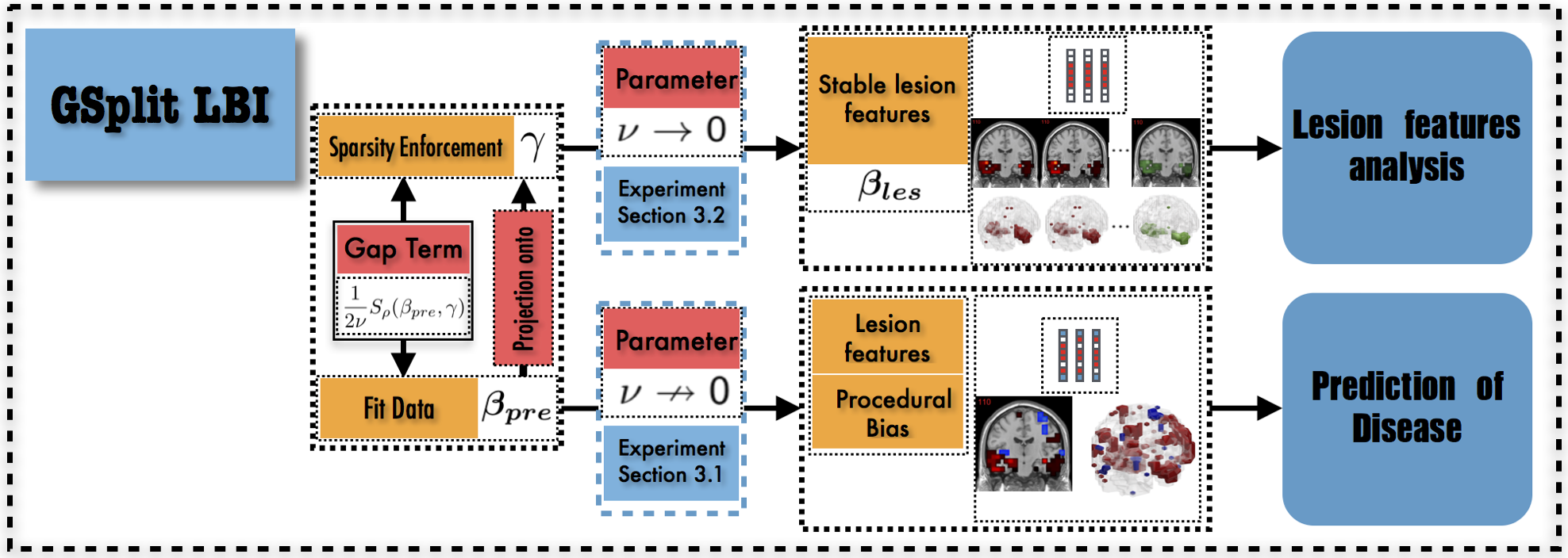
Figure 2: Illustration of GSplit LBI. The gap between $\beta_{pre}$ for fitting data and $\gamma$ for sparsity is controlled by $S_{\rho}(\beta_{pre},\gamma)$. The estimate $\beta_{les}$, as a projection of $\beta_{pre}$ on support set of $\gamma$, can be used for stable lesion features analysis when $\nu\to 0$ (Section 3.2). When $\nu\nrightarrow 0$ (Section 3.1) with appropriately large value, $\beta_{pre}$ can be used for prediction by capturing both lesion features and procedural bias.

To implement it, we generalize the Split Linearized Bregman Iteration (Split LBI) algorithm in [6] to our setting with generalized linear models (GLM) and the three types of structural sparsity above, hence called Generalized Split LBI (or GSplit LBI). Algorithm 1 describes the procedure with a new loss:

$$\ell(\beta_{0},\beta_{pre},\gamma;\{x_{i},y_{i}\}_{1}^{N},\nu):=\ell(\beta_{0},\beta_{pre};\{x_{i},y_{i}\}_{1}^{N})+\frac{1}{2\nu}S_{\rho}(\beta_{pre},\gamma),$$ (2.2)

where $\ell(\beta_{pre};\{x_{i},y_{i}\}_{1}^{N})$ is the negative log-likelihood function for GLM and $\nu>0$ tunes the strength of gap control. The algorithm returns a sequence of estimates as a regularization path, $\{\beta_{0}^{k},\beta_{pre}^{k},\gamma^{k},\beta_{les}^{k}\}_{k\geq 0}$. In particular, $\gamma^{k}$ shows a variety of sparsity levels and $\beta_{pre}^{k}$ is generically dense with different prediction powers. The projection of $\beta_{pre}^{k}$ onto the subspace with the same support of $\gamma^{k}$ gives estimate $\beta_{les}^{k}$, satisfying those a priori sparsity properties (sparse, 3D-smooth, nonnegative) and hence being regarded as the interpretable lesion features for AD. The remainder of this projection is heavily influenced by procedural bias; in this paper the non-zero elements in $\beta_{pre}^{k}$ which are negative (-1 denotes disease label) with comparably large magnitude are identified as procedural bias, while others with tiny values can be treated as nuisance or weak features. In summary, $\beta_{les}$ only selects lesion features; while $\beta_{pre}$ also captures additional procedural bias. Hence, such two kinds of features can be differentiated, as illustrated in Fig. 6.

Algorithm 1 GSplit LBI

1:  Input: Loss function $\ell(\beta_{0},\beta_{pre},\gamma;\{x_{i},y_{i}\}_{i=1}^{N},\nu)$, parameters $\nu$, $\rho$, $\kappa$, $\alpha>0$.

2:  Initialize: $k=0$, $t^{k}=0$, $\beta_{0}^{k}=0$, $\beta_{les}^{k}=0$, $\beta_{pre}^{k}=0$, $\gamma_{V}^{k}=0_{p}$, $\gamma_{G}^{k}=0_{m}$, $z_{V}^{k}=0_{p}$, $z_{G}^{k}=0_{m}$ and $S_{k}:=\mathrm{supp}(\gamma^{k})=\emptyset$.

3:  Iteration

4:   $\beta_{0}^{k+1}=\beta_{0}^{k}-\kappa\alpha\triangledown_{\beta_{0}}\thinspace\ell(\beta_{0}^{k},\beta_{pre}^{k},\gamma^{k};\{x_{i},y_{i}\}_{1}^{N},\nu)$

5:   $\beta_{pre}^{k+1}=\beta_{pre}^{k}-\kappa\alpha\triangledown_{\beta_{pre}}\thinspace\ell(\beta_{0}^{k},\beta_{pre}^{k},\gamma^{k};\{x_{i},y_{i}\}_{1}^{N},\nu)$

6:   $z^{k+1}=z^{k}-\alpha\triangledown_{\gamma}\thinspace\ell(\beta_{0}^{k},\beta_{pre}^{k},\gamma^{k};\{x_{i},y_{i}\}_{1}^{N},\nu)$

7:   $\gamma_{V}^{k+1}=\kappa\cdot\mathcal{S}^{+}(z_{V}^{k+1},1)$, where $\mathcal{S}^{+}(x,1)=\max(x-1,0)$

8:   $\gamma_{G}^{k+1}=\kappa\cdot\mathcal{S}(z_{G}^{k+1},1)$, where $\mathcal{S}(x,1)={\rm sign}(x)\cdot\max(|x|-1,0)$

9:   $\beta_{les}^{k+1}=P_{S_{k+1}}\beta_{pre}^{k+1}$, where $P_{S}=P_{ker(D_{S^{c}})}=I-D_{S^{c}}^{\dagger}D_{S^{c}}$

10:   $t^{k+1}=(k+1)\alpha$

11:  Output: $\{\beta_{0}^{k},\beta_{pre}^{k},\beta_{les}^{k},\gamma^{k}\}$, where $\gamma^{k+1}=\left[\begin{array}[]{cc}\gamma_{V}^{k+1}\\ \gamma_{G}^{k+1}\end{array}\right]$ and $z^{k+1}=\left[\begin{array}[]{cc}z_{V}^{k+1}\\ z_{G}^{k+1}\end{array}\right]$.

2.2 Setting the Parameters

A stopping time at $t^{k}$ (line 10) is the regularization parameter, which can be determined via cross-validation to minimize the prediction error [7]. Parameter $\rho$ is a tradeoff between geometric clustering and voxel sparsity. Parameter $\kappa$, $\alpha$ is damping factor and step size, which should satisfy $\kappa\alpha\leq\nu/\kappa(1+\nu\Lambda_{H}+\Lambda_{D}^{2})$ to ensure the stability of iterations. Here $\Lambda_{(\cdot)}$ denotes the largest singular value of a matrix and $H$ denotes the Hessian matrix of $\ell(\beta_{0},\beta_{pre};\{x_{i},y_{i}\}_{1}^{N})$.

Parameter $\nu$ balances the prediction task and sparsity enforcement in feature selection. In this paper, it is task-dependent, as shown in Fig. 6. For prediction of disease, $\beta_{pre}$ with appropriately larger value of $\nu$ may increase the prediction power by harnessing both lesion features and procedural bias. For lesion features analysis, $\beta_{les}$ with a small value of $\nu$ is helpful to enhance stability of feature selection. For details please refer to supplementary information.

3 Experimental Results

We apply our model to AD/NC classification (namely ADNC) and MCI (Mild Cognitive Impairment)/NC (namely MCINC) classification, which are two fundamental challenges in diagnosis of AD. The data are obtained from ADNI database, which is split into 1.5T and 3.0T (namely 15 and 30) MRI scan magnetic field strength datasets. The 15 dataset contains 64 AD, 208 MCI and 90 NC; while the 30 dataset contains 66 AD and 110 NC. DARTEL VBM pipeline [1] is then implemented to preprocess the data. Finally, the input features consist of 2,527 8$\times$8$\times$8 mm³ size voxels with average values in GM population template greater than 0.1. Experiments are designed on 15ADNC, 30ADNC and 15MCINC tasks.

3.1 Prediction and Path Analysis

10-fold cross-validation is adopted for classification evaluation. Under exactly the same experimental setup, comparison is made between GSplit LBI and other classifiers: SVM, MLDA (univariate model via t-test + LDA) [3], Graphnet [5], Lasso [10], Elastic Net, TV+L₁ and $n^{2}$GFL. For each model, optimal parameters are determined by grid-search. For GSplit LBI, $\rho$ is chosen from $\{1,2,...,10\}$, $\kappa$ is set to 10; $\alpha=\nu/\kappa(1+\nu\Lambda_{X}^{2}+\Lambda_{D}^{2})$; specifically, $\nu$ is set to 0.2 (corresponding to $\nu\nrightarrow 0$ in Fig. 6) . The regularization coefficient $\lambda$ is ranged in $\{0,0.05,0.1,...,0.95,1,10,10^{2}\}$ for lasso and $2^{\{-20,-19,...,0,...,20\}}$ for SVM. For other models, parameters are optimized from $\lambda:\thinspace\{0.05,0.1,...,0.95,1,10,10^{2}\}$ and $\rho:\thinspace\{0.5,1,..,10\}$(in addition, the mixture parameter $\alpha$: $\{0,0.05,...,0.95\}$ for Elastic Net).

Table 1: Comparison of GSplit LBI with other models

	MLDA	SVM	Lasso	Graphnet	Elastic Net	TV + $l_{1}$	$n^{2}$GFL	GSplit LBI ($\beta_{pre}$)
15ADNC	$85.06\%$	$83.12\%$	$87.01\%$	$86.36\%$	$88.31\%$	$83.77\%$	$86.36\%$	88.96%
30ADNC	$86.93\%$	$87.50\%$	$87.50\%$	$88.64\%$	$89.20\%$	$87.50\%$	$87.50\%$	90.91%
15MCINC	$61.41\%$	$70.13\%$	$69.80\%$	$72.15\%$	$70.13\%$	$73.83\%$	$69.80\%$	75.17%

The best accuracy in the path of GSplit LBI and counterpart are reported. Table 1 shows that $\beta_{pre}$ of our model outperforms that of others in all cases. Note that although our accuracies may not be superior to models with multi-modality data [8], they are the state-of-the-art results for only sMRI modality.

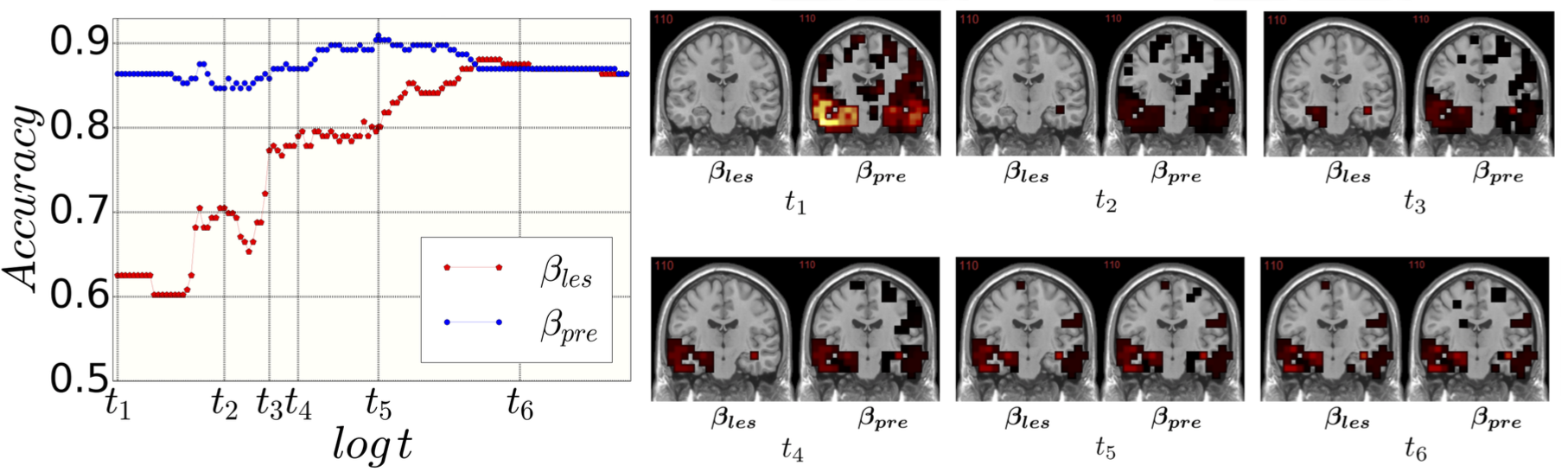
Figure 3: Left image: Accuracy of $(\beta_{pre},\beta_{les})$ vs $log\thinspace t$ ($t$: regularization parameter). Right image: Six 2-d brain slice images of selected degenerative voxels of $\beta_{les}$ and $\beta_{pre}$ are sorted orderly at $\{t_{1},...t_{6}\}$. As $t$ grows, $\beta_{pre}$ and $\beta_{les}$ identify similar lesion features.

The process of feature selection combined with prediction accuracy can be analyzed together along the path. The result of 30ADNC is used as an illustration in Fig. 3. We can see that $\beta_{pre}$ (blue curve) outperforms $\beta_{les}$ (red curve) in the whole path for additional procedural bias captured by $\beta_{pre}$. Specifically, at $\beta_{pre}$’s highest accuracy ($t_{5}$), there is a more than $8\%$ increase in prediction accuracy by $\beta_{pre}$. Early stopping regularization at $t_{5}$ is desired, as $\beta_{pre}$ converges to $\beta_{les}$ in prediction accuracy with overfitting when $t$ grows. Recall that positive (negative) features represent degenerate (enlarged) voxels. In each fold of $\beta_{pre}$ at $t_{5}$, the commonly selected voxels among top 150 negative (enlargement) voxels are identified as procedural bias shown in Fig. 1, where most of these GM voxels are enlarged and located near lateral ventricle or subarachnoid space etc., possibly due to enlargement of CSF space in those locations that are different from the lesion features.

3.2 Lesion Features Analysis

To quantitatively evaluate the stability of selected lesion features, multi-set Dice Coefficient (mDC) [4, 13] is applied as a measurement. The 30ADNC task is again applied as an example, the mDC is computed for $\beta_{les}$ which achieves highest accuracy by 10-fold cross-validation. As shown from Table 2, when $\nu=0.0002$ (corresponding to $\nu\to 0$ in Fig. 6), the $\beta_{les}$ of our model can obtain more stable lesion feature selection results than other models with comparable prediction power. Besides, the average number of selected features (line 3 in Table 2) are also recorded . Note that although elastic net is of slightly higher accuracy than $\beta_{les}$, it selects much more features than necessary.

Table 2: mDC comparison between GSplit LBI and other models

	Lasso	Elastic Net	Graphnet	TV + $l_{1}$	$n^{2}$ GFL	GSplit LBI ($\beta_{les}$)
Accuracy	$87.50\%$	$89.20\%$	$88.64\%$	$87.50\%$	$87.50\%$	$88.64\%$
mDC	0.1992	0.5631	0.6005	0.5824	0.5362	0.7805
$\sum_{k=1}^{10}\thinspace|S(k)|/10$	50.2	777.8	832.6	712.6	443.9	129.4

For the meaningfulness of selected lesion features, they are shown in Fig. 4 (a)-(c), located in hippocampus, parahippocampal gyrus and medial temporal lobe etc., which are believed to be early damaged regions for AD patients.

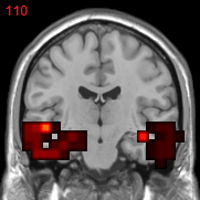
(a) fold 2

(b) fold 10

(c) overlap

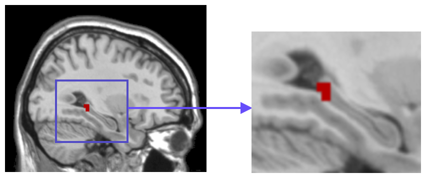
(d) coarse-to-fine

Figure 4: (a)-(c): Stability of selected lesion features of $\beta_{les}$ shown in 2-d 110 slice brain images when $\nu=0.0002$. (a)-(b): Results of fold 2 and fold 10. (c): The overlapped features in 10 folds. (d): The 2-d slice brain image of selected voxels with $2\times 2\times 2$ $mm^{3}$ using coarse-to-fine approach.

To further investigate the locus of lesion features, we conduct a coarse-to-fine experiment. Specifically, we project the selected overlapped voxels of $8\times 8\times 8$ $mm^{3}$ size (shown in Fig. 4 (c)) onto MRI image with more finer scale voxels, i.e. in size of $2\times 2\times 2$ $mm^{3}$. Totally 4,895 voxels are served as input features after projection. Again, the GSplit LBI is implemented using 10-fold cross-validation. The prediction accuracy of $\beta_{pre}$ is $90.34\%$ and on average 446.6 voxels are selected by $\beta_{les}$. As desired, these voxels belong to parts of lesion regions, such as those located in hippocampal tail, as shown in Fig. 4 (d).

4 Conclusions

In this paper, a novel iterative dual task algorithm is proposed to incorporate both disease prediction and lesion feature selection in neuroimage analysis. With variable splitting term, the estimators for prediction and selecting lesion features can be separately pursued and mutually monitored under a gap control. The gap here is dominated by procedural bias, some specific features crucial for prediction yet ignored in a priori disease knowledge. With experimental studies conducted on 15ADNC, 30ADNC and 15MCINC tasks, we have shown that the leverage of procedural bias can lead to significant improvements in both prediction and model interpretability. In future works, we shall extend our model to other neuroimaging applications including multi-modality data.

Acknowledgements. This work was supported in part by 973-2015CB351800, 2015CB85600, 2012CB825501, NSFC-61625201, 61370004, 11421110001 and Scientific Research Common Program of Beijing Municipal Commission of Education (No. KM201610025013).

Supplementary Information

Appendix A Notation

For matrix $A$, $A_{J}$ represents the submatrix of $A$ indexed by $J$. $A^{{\dagger}}$ denotes the Moore-Penrose pseudoinverse of $A$. Suppose $A\in R^{n\times n}$, $\|A\|_{\Sigma}:=\mathrm{trace}(A)=\sum_{i=1}^{n}A_{i,i}$. Besides, $\tilde{\beta}$ and $\beta$ are used to represent $\beta_{les}$ and $\beta_{pre}$ respectively in what follows.

Appendix B Model selection consistency

Consider recovery from generalized linear model(GLM) of $\beta^{\star}\in R^{p}$ which satisfies structural sparsity after linearly transformed by $D\in R^{m\times p}$:

$$P(y|x,\beta^{\star})\propto exp(\frac{x^{T}\beta^{\star}\cdot y-\psi(x^{T}\beta^{\star})}{d(\sigma)})$$

$$s.t.\quad \gamma^{\star}=D\beta^{\star}\thinspace(S:=supp(\gamma^{\star}),\thinspace s=|S|,\thinspace s<<m)$$ (B.1)

where $\psi:R\to R$ is link function and $d(\sigma)$ is known parameter related to the variance of distribution.

Under linear model with $\psi(t)=t^{2}$ and $d(\sigma)=\sigma^{2}$ in B.1, our model GSplit LBI degenerates to Split LBI [6]. Recently, it’s proved in [6] that the Split LBI may achieve model selection consistency under weaker conditions than generalized lasso [11, 12] if $\nu$ is large enough. We claim that this property can also be shared by logit model.

To understand why Gsplit LBI can achieve better model selection consistency, note that the variable splitting term projects solution vector $\beta$ into higher dimensional space $(\beta,\gamma)$ with $\beta$ fitting data and $\gamma$ being structural sparse. This will make it easier for the subspace of $\gamma_{S^{c}}$ to decorrelate with the subspace of $(\beta,\gamma_{S})$, especially when $\nu$ increases, which sheds light on better performance of Split LBI to recover true signal set $S$. What’s more important, the property may also be shared by logit model when $y=\{\pm 1\}$, $d(\sigma)=1$ and $\psi(t)=log(1+exp(t))$. Concretely speaking, we use $\theta_{S^{c},(\beta,S)}(\nu)$ to denote the angle between subspace of $\gamma_{S^{c}}$ and that of $(\beta,\gamma_{S})$, the definition of which is:

$$\theta_{S^{c},(\beta,S)}(\nu):=\mathrm{arccos}\thinspace(\frac{\|P_{A_{(\beta,S)}}A_{S^{c}}\|_{F}}{\|A_{S^{c}}\|_{F}})=\mathrm{arccos}\thinspace(\sqrt{\frac{\|H_{S^{c},(\beta,S)}H^{\dagger}_{(\beta,S),(\beta,S)}H_{(\beta,S),S^{c}}\|_{\Sigma}}{\|H_{S^{c},S^{c}}\|_{\Sigma}}})$$ (B.2)

Where $A:=\left[\begin{array}[]{cc}A_{(\beta,S)}&A_{S^{c}}\end{array}\right]$ and $H:=\triangledown^{2}_{\beta,\gamma}\thinspace l(\beta,\gamma)=A^{T}A=\left[\begin{array}[]{cc}H_{(\beta,S),(\beta,S)}&H_{(\beta,S),S^{c}}\\ H_{S^{c},(\beta,S)}&H_{S^{c},S^{c}}\end{array}\right]$.

Remark 1

For linear model, $A=\triangledown_{\beta,\gamma}\thinspace l(\beta,\gamma)$ with

$$A_{(\beta,S)}=\left[\begin{array}[]{cc}X&0_{n\times s}\\ -D_{S}/\sqrt{\nu}&I_{(S,S)}/\sqrt{\nu}\\ -D_{S^{c}}/\sqrt{\nu}&0_{(p-s)\times s}\end{array}\right]\quad A_{S^{c}}=\left[\begin{array}[]{cc}0_{n\times(p-s)}\\ 0_{s\times(p-s)}\\ I_{(S^{c},S^{c})}/\sqrt{\nu}\end{array}\right]$$ (B.9)

There is no explicit definition for $A$ for logit model, however $\theta_{S^{c},(\beta,S)}(\nu)$ can be computed through Hessian matrix $H$ in equation B.9.

We claim that $\theta_{S^{c},(\beta,S)}(\nu)$ will increase as $\nu$ becomes larger under some conditions. See theorem B.1 for details.

Theorem B.1

Under linear model and logit model, $lim_{\nu\to+\infty}\theta_{S^{c},(\beta,S)}(\nu)=90^{\circ}$ if and only if $\mathrm{Im}(D_{S^{c}}^{T})\subseteq\mathrm{Im}(X^{T})$.

Remark 2

In [6], it’s been proved that the necessary condition for sign-consistency is $IRR(\nu)<1$. For uniqueness of model, we also assume that $ker(X)$ $\cap$ $ker(D_{S^{c}})$ $\subseteq ker(D_{S})$. Combined with $\mathrm{Im}(D_{S^{c}}^{T})\subseteq\mathrm{Im}(X^{T})\iff ker(X)\subseteq ker(D_{S^{c}})$, we have that $ker(X)\subseteq ker(D_{S})$, which is the sufficient and necessary condition for the hold of $\lim_{\nu\to\infty}\mathrm{IRR}(\nu)\to 0$. Hence, this is another way to understand why GSplit LBI can achieve better model selection consistency.

Proof

We firstly prove the case under linear model. Denoted $A:=\nu X^{\star}X+D^{T}D$ where $X\in R^{n\times p}$ and $X^{\star}=X/n$. Note that:

$$H_{(\beta,S),(\beta,S)}=QLQ^{T},\quad H_{S^{c},(\beta,S)}=\left[\begin{array}[]{cc}D_{S^{c}}/\nu&0\end{array}\right]$$

where:

$$Q=\left[\begin{array}[]{cc}I_{p}&0\\ -D_{S}A^{\dagger}&I_{s}\end{array}\right],\quad L=\left[\begin{array}[]{cc}A/\nu&0\\ 0&(I_{s}-D_{S}A^{\dagger}D_{S}^{T})/\nu\end{array}\right]$$ (B.15)

Then we have:

$$H_{S^{c},(\beta,S)}H^{\dagger}_{(\beta,S),(\beta,S)}H_{(\beta,S),S^{c}}=H_{S^{c},(\beta,S)}QL^{\dagger}Q^{T}H_{(\beta,S),S^{c}}=\frac{1}{\nu}D_{S^{c}}A^{\dagger}D_{S^{c}}^{T}$$ (B.16)

Substituting equation B.16 into the second equation of B.2, we have:

$$\mathrm{cos}^{2}(\theta_{S^{c},(\beta,S)}(\nu))=\frac{\|D_{S^{c}}A^{\dagger}D_{S^{c}}\|_{\Sigma}}{\|H_{S^{c},S^{c}}\|_{\Sigma}}=\frac{\|D_{S^{c}}A^{\dagger}D_{S^{c}}\|_{\Sigma}}{m-s}$$ (B.17)

Denote $e_{i}\in R^{m-s}$ as the vector with the $i^{th}$ element being 1 and left being 0. Then equation B.17 is equivalent to:

$$\mathrm{cos}^{2}(\theta_{S^{c},(\beta,S)}(\nu))(m-s)=\Sigma_{i=1}^{p}d_{i}^{T}A^{\dagger}d_{i}$$ (B.18)

where $d_{i}:=D_{S^{c}}^{T}e_{i}$. Suppose the compact singular value decomposition of $X/\sqrt{n}:=U\Lambda V^{T}$, and $(V,\tilde{V})$ be an orthogonal square matrix. Suppose the compact singular value decomposition of $D\tilde{V}:=U_{1}\Lambda_{1}V_{1}^{T}$. If $\mathrm{Im}(D_{S^{c}}^{T})\subseteq\mathrm{Im}(X^{T})$, then $\exists f_{i}$, such that $d_{i}=Vf_{i}$, hence,

$$d_{i}^{T}(\nu X^{\star}X+D^{T}D)^{\dagger}d_{i} =d_{i}^{T}\begin{pmatrix}V&\tilde{V}\end{pmatrix}\left(\begin{pmatrix}V^{T}\\ \tilde{V}^{T}\end{pmatrix}(\nu X^{\star}X+D^{T}D)\begin{pmatrix}V&\tilde{V}\end{pmatrix}\right)^{{\dagger}}\begin{pmatrix}V^{T}\\ \tilde{V}^{T}\end{pmatrix}d_{i}$$

$$=f_{i}^{T}(\nu\Lambda^{2}+V^{T}D^{T}DV)^{-1}f_{i}\to 0,\ as\ \nu\to\infty$$ (B.19)

Combined with equation B.18, it’s then easy to obtain that $\mathrm{cos}^{2}(\theta_{S^{c},(\beta,S)}(\nu))\to 0$ as $\nu\to+\infty$. On the contrary, if $\exists\thinspace a$ such that $D_{S^{c}}^{T}a\notin\mathrm{Im}(X^{T})$, then there $\exists\thinspace i^{\star}$ such that $d_{i^{\star}}\notin\mathrm{Im}(X^{T})$. This means that for $d_{i^{\star}}$, there $\exists\thinspace f_{1,i^{\star}},f_{2,i^{\star}}\neq 0$ such that $d_{i^{\star}}=Vf_{1,i^{\star}}+\tilde{V}f_{2,i^{\star}}$. Then we have

$$d_{i^{\star}}^{T}(\nu X^{\star}X+D^{T}D)^{\dagger}d_{i^{\star}}\geq f_{2,i^{\star}}^{T}(\tilde{V}^{T}D^{T}D\tilde{V})^{{\dagger}}f_{2,i^{\star}}=f_{2,i^{\star}}^{T}V_{1}\Lambda_{1}^{-2}V_{1}^{T}f_{2,i^{\star}}$$

does not equal to $0\iff f_{2,i^{\star}}^{T}V_{1}\Lambda_{1}^{2}V_{1}^{T}f_{2,i^{\star}}=f_{2,i^{\star}}^{T}\tilde{V}^{T}D^{T}D\tilde{V}f_{2,i^{\star}}\neq 0$. Since

$$f_{2,i^{\star}}^{T}\tilde{V}^{T}D^{T}D\tilde{V}f_{2,i^{\star}}\geq f_{2,i^{\star}}^{T}\tilde{V}^{T}d_{i^{\star}}d_{i^{\star}}^{T}f_{2,i^{\star}}=(f_{2,i^{\star}}^{T}f_{2,i^{\star}})^{2}>0$$

From equation B.18, we can obtain that:

$$\mathrm{cos}^{2}(\theta_{S^{c},(\beta,S)}(\nu))(m-s)\geq d_{i^{\star}}^{T}A^{\dagger}d_{i^{\star}}\neq 0$$

which means the $\theta_{S^{c},(\beta,S)}(\nu)\to 0$ does not hold when $\nu\to+\infty$. The proof is then completed under linear model. Under logit model, the definition of $A$ is modified to $A:=\nu X^{\star}W(\{x_{i},\beta\}_{i=1}^{p})X+D^{T}D$ where $W(\{x_{i},\beta\}_{i=1}^{p})$ is a diagonal matrix with each diagonal element equals to $\frac{exp(x_{i}^{T}\beta)}{(1+exp(x_{i}^{T}\beta))^{2}}$, the left proof is almost the same with that of linear model.

An simulation experiment is conducted to illustrate this idea. In more detail, $n=100$ and $p=80$, $D=I$ and $X\in R^{n\times p}$ and $X_{i,j}\sim N(0,1)$. $\beta^{\star}_{i}=2$ for $1\leq i\leq 4$, $\beta^{\star}_{i}=-2$ for $5\leq i\leq 8$ and 0 otherwise, $y$ is generated by both linear model $y=X\beta^{\star}+\epsilon$ with $\epsilon\sim N(0,1)$ and logit model given $X$ and $\beta^{\star}$. We simulated for 100 times and average $\theta_{S^{c},(\beta,S)}(\nu)$ is then computed, which is shown in the left image in figure 5. We can see that $\theta_{S^{c},(\beta,S)}(\nu)$ increases when $\nu$ becomes larger, as illustrated in right image in figure 5, and converges to $90^{\circ}$ when $\nu\to+\infty$.

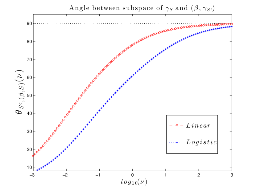
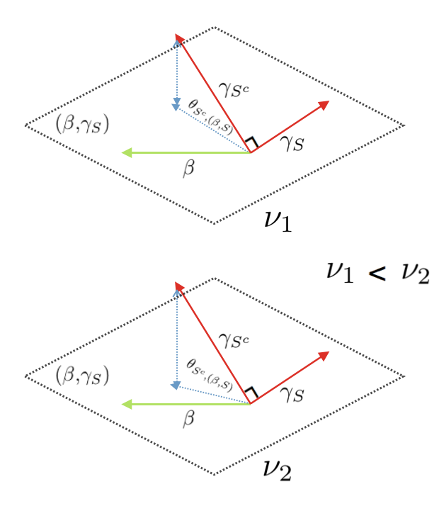
Figure 5: Left image: The $\theta_{S^{c},(\beta,S)}(\nu)$ curve of logit model and linear model. Right image: Illustration of $\theta_{S^{c},(\beta,S)}(\nu)$ and it monotonically increase v.s. $\nu$.

The average AUC and estimation of $\beta^{\star}$ of Gsplit LBI with different $\nu$ compared with those of genlasso are also computed. Table 3 shows better AUC with the increase of $\nu$ before $\nu=100$. As we can see from the algorithm in the paper that $\tilde{\beta}$ is the projection of $\beta$ onto the support set of $\gamma$. Hence it is equivalent to say that better model selection of $\tilde{\beta}$ can be achieved as $\nu$ increases.

However, the excessively large value of $\nu$ will lower the signal-to-noise ratio, which is also crucial for model selection consistency and prediction estimation. It’s shown in [6] that $\nu$ determines the trade-off between model selection consistency and estimation of $\beta^{\star}$. Also, the irrepresentable condition(IRR) can be satisfied as long as $\nu$ is large enough. If $\nu$ continuously increase, it will deteriorate the estimation of $\beta^{\star}$, prediction estimation and even AUC. In our experiment the same phenomena can be observed, i.e. the estimation of $\tilde{\beta}$ and $\beta$ get worse if $\nu$ increases from 10 and 100, respectively; when $\nu=100$, AUC even decreases.

Table 3: Comparison between Gsplit LBI with different $\nu$ and genlasso in terms of AUC, $\|\tilde{\beta}-\beta^{\star}\|_{2}$, $\|\beta-\beta^{\star}\|_{2}$, $\|X\tilde{\beta}-X\beta^{\star}\|_{2}$ and $\|X\beta-X\beta^{\star}\|_{2}$.

Model	Gsplit LBI						genlasso
$\nu$	0.02	0.1	1	5	10	100	-
AUC	0.9531	0.98194	0.98514	0.98791	0.98792	0.98590	0.97915
$\|\tilde{\beta}-\beta^{\star}\|_{2}$	4.9079	4.9015	4.8513	4.8495	4.8473	5.3578	-
$\|\beta-\beta^{\star}\|_{2}$	3.9187	3.8993	3.7619	3.6814	3.7129	5.1540	4.9113
$\|X\tilde{\beta}-X\beta^{\star}\|_{2}$	47.0224	46.9625	46.6784	46.9158	47.0098	52.2737	-
$\|X\beta-X\beta^{\star}\|_{2}$	37.3496	37.0962	35.4987	34.6423	34.8514	49.61020	50.6408

Appendix C Relationship between $\beta$ and $\tilde{\beta}$

The estimate $\tilde{\beta}$, as a projection of $\beta$ onto the subspace of $\gamma$, can select features that satisfy structural sparsity. Following the Linearized Bregman Iteration [14], $\beta$ and $\tilde{\beta}$ will be more similar on features selected by $\tilde{\beta}$. In more detail, note that when $t=0$, $\tilde{\beta}(t)=0$ and $\beta(t)$ is the graph laplacian regularizer with penalty factor $\frac{1}{2\nu}$. As $t$ progresses, the gap between $\beta(t)$ and $\tilde{\beta}(t)$ will decrease in terms of $\|\beta(t)-\tilde{\beta}(t)\|_{2}$ for every $\nu$, as shown in figure 6.

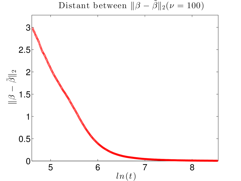
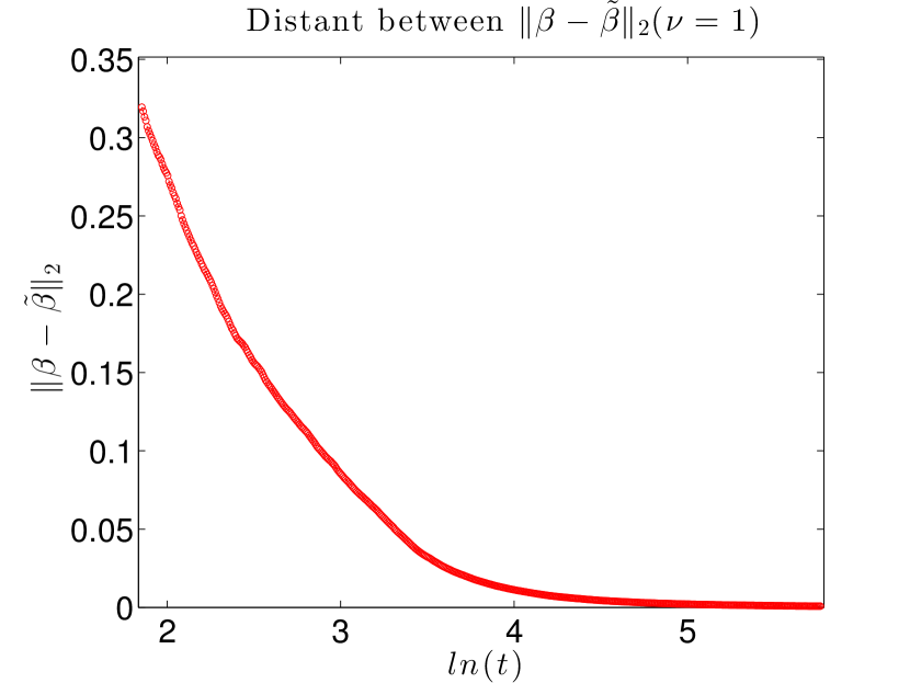
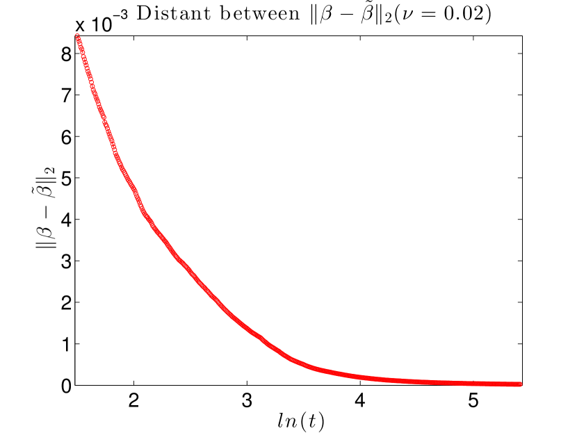
Figure 6: $\|\beta-\tilde{\beta}\|_{2}$ in the regularized solution path when $\nu=100,1,0.02$. As $\nu$ decreases, the distance of $\beta(t)$ and $\tilde{\beta}(t)$ are tended to be with smaller distance.

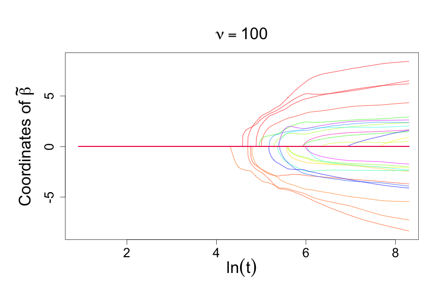
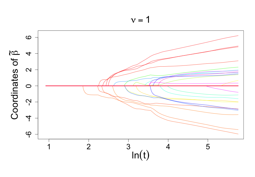
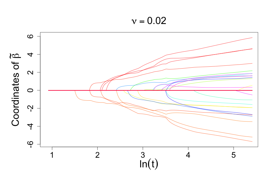
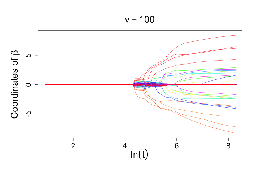
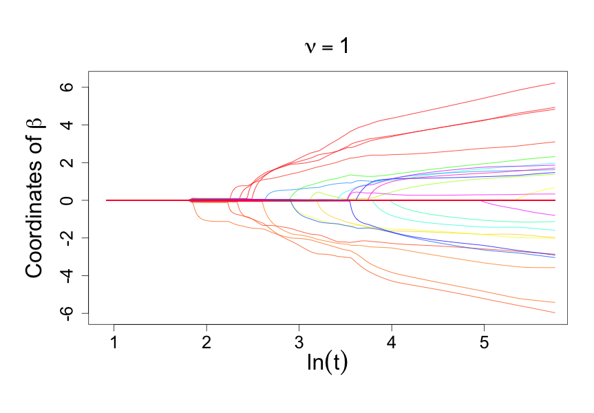
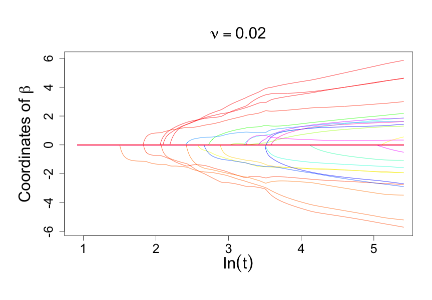
Figure 7: Comparison of regularized solution path between $\beta$ and $\tilde{\beta}$ when $\nu=100,1,0.02$. They look more similar with each other as $\nu$ decreases.

Since $\|\beta(t)-\tilde{\beta}(t)\|_{2}\to 0$ as $t\to+\infty$ and $\tilde{\beta}$ is sparse, it follows that $\beta$ will approximate to $\tilde{\beta}$ on those selected features. In addition to these selected features, before convergence to $\tilde{\beta}$, $\beta$ can capture other features to better fit data(minimize training error), especially for those ones that significantly correlated with data.

Appendix D Choice of $\nu$

The choice of $\nu$ is task-dependent. For stable feature selection, $\nu$ with rather ”small” value is suggested. It’s noted that $\beta-\tilde{\beta}\to 0$ as $\nu\to 0^{+}$, which is reflected by $l_{2}$ norm and regularized solution path shown in figure 6, 7. In this case, the estimator $\tilde{\beta}$ will be constrained in comparably lower dimension space, therefore it may fit data with more stability, notwithstanding $\beta$ have no ability to select other features.

For prediction estimation, the appropriately large value of $\nu$ is preferred. On one hand, when $\nu$ is appropriately large, the ability of selecting features with better model selection consistency can be achieved and $\beta$ will share closer values on these selected features as $t$ progress, as shown in figure 7. On the other hand, $\beta$ may increase the ability of fitting data by having other features being non-zeros as long as $\nu$ is not too small. In fact, it is shown in table 3 that comparable results can be given as long as $\nu$ belongs to a reasonable range of values(0.1-10 in this case).

Appendix E IDS of ADNI subject used in our experiments

Subject	ID	Class	Subject	ID	Class	Subject	ID	Class
123_S_0094	9655	15AD	027_S_0408	14964	15MCI	072_S_0315	12559	15NC
123_S_0088	9788	15AD	137_S_0481	15044	15MCI	137_S_0301	12584	15NC
098_S_0149	10146	15AD	027_S_0417	15148	15MCI	002_S_0295	13722	15NC
032_S_0147	10404	15AD	053_S_0507	15315	15MCI	037_S_0327	13802	15NC
123_S_0162	10962	15AD	094_S_0531	15431	15MCI	027_S_0403	14146	15NC
128_S_0216	11101	15AD	033_S_0567	15459	15MCI	137_S_0459	14178	15NC
128_S_0167	11203	15AD	127_S_0394	15510	15MCI	002_S_0413	14437	15NC
005_S_0221	11604	15AD	033_S_0514	15605	15MCI	068_S_0473	14483	15NC
014_S_0328	12327	15AD	033_S_0513	15622	15MCI	116_S_0360	14623	15NC
007_S_0316	12616	15AD	130_S_0460	15711	15MCI	133_S_0488	14838	15NC
021_S_0343	12979	15AD	098_S_0542	15848	15MCI	133_S_0493	14848	15NC
014_S_0356	13004	15AD	007_S_0414	15875	15MCI	014_S_0520	15299	15NC
032_S_0400	13525	15AD	031_S_0568	15885	15MCI	014 _S_0519	15323	15NC
116_S_0370	14122	15AD	037_S_0501	15916	15MCI	116 _S_0382	15347	15NC
127_S_0431	15497	15AD	037_S_0552	15970	15MCI	128_S_0500	15366	15NC
031_S_0554	15994	15AD	130_S_0423	16196	15MCI	010_S_0419	15415	15NC
128_S_0517	16150	15AD	014_S_0557	16304	15MCI	131_S_0436	15674	15NC
116_S_0487	16377	15AD	033_S_0511	16314	15MCI	128_S_0522	15821	15NC
002_S_0619	16392	15AD	130_S_0449	16351	15MCI	033_S_0516	15860	15NC
131_S_0497	16666	15AD	027_S_0461	16467	15MCI	002_S_0559	15948	15NC
021_S_0642	17632	15AD	128_S_0608	16503	15MCI	014_S_0548	16024	15NC
033_S_0739	19175	15AD	128_S_0611	16766	15MCI	128_S_0545	16090	15NC
100_S_0743	19585	15AD	053_S_0621	16864	15MCI	031_S_0618	16598	15NC
033_S_0724	19772	15AD	037_S_0566	16886	15MCI	010_S_0420	17078	15NC
128_S_0740	19990	15AD	037_S_0539	17018	15MCI	126 _S_0506	17184	15NC
021_S_0753	20169	15AD	137_S_0443	17030	15MCI	005_S_0610	17303	15NC
137_S_0796	23112	15AD	005_S_0546	17056	15MCI	006_S_0484	17377	15NC
029_S_0836	23231	15AD	137_S_0631	17109	15MCI	014_S_0558	17400	15NC
100_S_0747	23581	15AD	027_S_0644	17157	15MCI	021_S_0647	17668	15NC
127_S_0754	23787	15AD	133_S_0629	17596	15MCI	137 _S_0686	17813	15NC
012_S_0803	24863	15AD	021_S_0626	17687	15MCI	032_S_0677	17820	15NC
033_S_0889	25026	15AD	098_S_0667	17702	15MCI	002_S_0685	18211	15NC
126_S_0891	25172	15AD	052_S_0671	17849	15MCI	094_S_0711	18589	15NC
005_S_0929	25645	15AD	014_S_0563	17876	15MCI	127_S_0684	18896	15NC
006_S_0547	25816	15AD	007_S_0698	18363	15MCI	033_S_0734	19155	15NC
002_S_0955	26170	15AD	133_S_0638	18672	15MCI	033_S_0741	19258	15NC
130_S_0956	27032	15AD	033_S_0723	19014	15MCI	094_S_0692	19567	15NC
053_S_1044	27782	15AD	032_S_0718	19035	15MCI	009 _S_0751	20013	15NC
133_S_1055	29381	15AD	126_S_0708	19089	15MCI	116_S_0648	20370	15NC
100_S_1062	29579	15AD	128_S_0715	19225	15MCI	129_S_0778	20543	15NC
029_S_1056	30618	15AD	033_S_0725	19404	15MCI	029_S_0824	23213	15NC
029_S_0999	31239	15AD	137_S_0669	19419	15MCI	116_S_0657	23350	15NC
006_S_0653	31252	15AD	116_S_0649	19516	15MCI	006_S_0731	23468	15NC
014_S_1095	31576	15AD	130_S_0505	19701	15MCI	029_S_0845	24249	15NC
094_S_1090	31678	15AD	137_S_0722	19707	15MCI	009_S_0862	25128	15NC
021_S_1109	31784	15AD	126_S_0709	19754	15MCI	098_S_0896	25255	15NC
024_S_1171	35190	15AD	128_S_0770	19907	15MCI	033_S_0923	25427	15NC
133_S_1170	35211	15AD	014_S_0658	20003	15MCI	130_S_0886	25455	15NC
031_S_1209	36178	15AD	137_S_0668	20202	15MCI	006_S_0498	25790	15NC
130_S_1201	36269	15AD	137_S_0800	20500	15MCI	052_S_0951	26642	15NC
027_S_1081	37145	15AD	002_S_0782	20519	15MCI	130_S_0969	26688	15NC
126_S_1221	37339	15AD	130_S_0783	20794	15MCI	021_S_0984	27056	15NC
029_S_1184	37350	15AD	116_S_0752	23097	15MCI	024_S_0985	27607	15NC
027_S_1254	37859	15AD	068_S_0802	23389	15MCI	024_S_1063	28111	15NC
130_S_1290	38395	15AD	133_S_0792	23444	15MCI	033_S_1098	30304	15NC
033_S_1285	38593	15AD	006_S_0675	23644	15MCI	010_S_0472	30481	15NC
033_S_1283	38617	15AD	031_S_0821	23658	15MCI	137_S_0972	31702	15NC
033_S_1308	40114	15AD	133_S_0771	23876	15MCI	033_S_1086	32054	15NC
024_S_1307	41527	15AD	133_S_0727	23939	15MCI	130_S_1200	36281	15NC
007_S_1339	42344	15AD	027_S_0835	24138	15MCI	116_S_1232	37848	15NC
130_S_1337	42930	15AD	031_S_0830	24281	15MCI	027_S_0120	10933	15NC
127_S_1382	45060	15AD	029_S_0878	24533	15MCI	068_S_0127	11133	15NC
094_S_1397	51790	15AD	136_S_0695	24585	15MCI	068_S_0210	11235	15NC
094_S_1402	54220	15AD	031_S_0867	24962	15MCI	136_S_0186	11335	15NC
136_S_0299	15181	30AD	033_S_0906	25053	15MCI	009_S_0842	24339	15NC
136_S_0426	16172	30AD	033_S_0922	25092	15MCI	029_S_0843	24406	15NC
018_S_0335	16560	30AD	012_S_0932	25150	15MCI	032_S_1169	34067	15NC
136_S_0300	16719	30AD	137_S_0825	25272	15MCI	018_S_0055	9136	15NC
018_S_0633	19093	30AD	116_S_0834	25467	15MCI	100_S_0015	8390	30NC
012_S_0689	19210	30AD	094_S_0921	25498	15MCI	136_S_0196	14236	30NC
126_S_0606	20487	30AD	136_S_0873	25559	15MCI	136_S_0086	14712	30NC
131_S_0691	20681	30AD	100_S_0930	25618	15MCI	018_S_0369	15110	30NC
005_S_0814	24734	30AD	133 _S_0912	26000	15MCI	131_S_0441	15959	30NC
002_S_0816	25405	30AD	032_S_0978	26407	15MCI	032_S_0479	16652	30NC
127_S_0844	29230	30AD	100_S_0892	26443	15MCI	018_S_0425	17168	30NC
002_S_1018	33832	30AD	052_S_0952	26661	15MCI	126_S_0405	17177	30NC
031_S_4024	228879	30AD	053_S_0919	26739	15MCI	005_S_0553	17619	30NC
016_S_4009	240946	30AD	068_S_0872	27450	15MCI	126_S_0605	17639	30NC
094_S_4089	242719	30AD	094_S_1015	28005	15MCI	005_S_0602	19615	30NC
006_S_4153	248517	30AD	133_S_1031	28152	15MCI	012_S_1009	28962	30NC
003_S_4136	250173	30AD	127_S_0925	28165	15MCI	012_S_1212	37403	30NC
003_S_4152	253760	30AD	137_S_0994	28269	15MCI	007_S_1206	37761	30NC
098_S_4215	255843	30AD	009_S_1030	28514	15MCI	068_S_1191	38370	30NC
098_S_4201	256178	30AD	100_S_0995	28877	15MCI	007_S_1222	38482	30NC
006_S_4192	258594	30AD	027_S_1045	28947	15MCI	094_S_1241	41449	30NC
019_S_4252	258947	30AD	136_S_0874	29140	15MCI	002_S_1261	41799	30NC
024_S_4280	261332	30AD	127_S_1032	29177	15MCI	002_S_1280	41806	30NC
094_S_4282	261855	30AD	126_S_0865	29243	15MCI	052_S_1251	43812	30NC
029_S_4307	267595	30AD	031_S_1066	29388	15MCI	100_S_1286	45761	30NC
016_S_4353	267937	30AD	052_S_0989	29525	15MCI	094_S_1267	46457	30NC
109_S_4378	270669	30AD	137_S_0973	29650	15MCI	131_S_1301	49328	30NC
126_S_4494	281605	30AD	012_S_1033	29964	15MCI	098_S_4003	224603	30NC
127_S_4500	283515	30AD	033_S_1116	30317	15MCI	098_S_4018	228788	30NC
007_S_4568	287472	30AD	029_S_1073	30359	15MCI	031_S_4021	229148	30NC
006_S_4546	287994	30AD	029_S_1038	30395	15MCI	012_S_4026	238532	30NC
130_S_4589	291219	30AD	052_S_1054	30580	15MCI	098_S_4050	238615	30NC
016_S_4591	292433	30AD	037_S_1078	30960	15MCI	016_S_4097	243556	30NC
016_S_4583	294209	30AD	010_S_0422	31015	15MCI	016_S_4952	337793	30NC
014_S_4615	294334	30AD	012_S_0917	31725	15MCI	016_S_4121	246002	30NC
130_S_4641	295961	30AD	006_S_1130	31799	15MCI	006_S_4150	249403	30NC
130_S_4660	300034	30AD	126_S_1077	31850	15MCI	127_S_4148	250137	30NC
019_S_4549	300335	30AD	037_S_0588	32151	15MCI	003_S_4119	250894	30NC
126_S_4686	300818	30AD	052_S_1168	32349	15MCI	127_S_4198	254320	30NC
005_S_4707	304663	30AD	010_S_0904	32497	15MCI	002_S_4213	254582	30NC
021_S_4718	304749	30AD	002_S_1155	33393	15MCI	031_S_4218	255978	30NC
018_S_4733	306069	30AD	029_S_0871	33717	15MCI	002_S_4225	257270	30NC
130_S_4730	306384	30AD	127_S_1140	33761	15MCI	002_S_4262	259653	30NC
137_S_4756	307118	30AD	029_S_0914	33775	15MCI	941_S_4100	259781	30NC
027_S_4801	314034	30AD	100_S_1154	34258	15MCI	002_S_4264	259796	30NC
027_S_4802	317195	30AD	094_S_1188	34619	15MCI	021_S_4276	260047	30NC
006_S_4867	322012	30AD	012_S_1165	35052	15MCI	029_S_4290	260425	30NC
016_S_4887	325649	30AD	133_S_0913	35171	15MCI	098_S_4275	261459	30NC
007_S_4911	328196	30AD	012_S_1175	35342	15MCI	094_S_4234	261531	30NC
021_S_4924	331257	30AD	126_S_1187	36364	15MCI	018_S_4257	262076	30NC
137_S_4756	332930	30AD	009_S_1199	36373	15MCI	136_S_4269	264215	30NC
127_S_4940	335512	30AD	029_S_1215	37129	15MCI	029_S_4279	265980	30NC
027_S_4938	336926	30AD	116_S_0890	37182	15MCI	021_S_4335	266174	30NC
027_S_4962	338558	30AD	100_S_1226	37251	15MCI	130_S_4343	266217	30NC
130_S_4982	341787	30AD	005_S_1224	37284	15MCI	018_S_4349	266625	30NC
130_S_4984	342274	30AD	037_S_1225	37364	15MCI	129_S_4369	267405	30NC
130_S_4971	342338	30AD	029_S_1218	37373	15MCI	130_S_4352	267711	30NC
127_S_4992	342697	30AD	027_S_1213	37393	15MCI	129_S_4371	268462	30NC
019_S_5012	343916	30AD	127_S_1210	38319	15MCI	018_S_4313	268930	30NC
019_S_5019	345663	30AD	116_S_1243	38462	15MCI	019_S_4367	269273	30NC
002_S_5018	346242	30AD	033_S_1309	38837	15MCI	007_S_4387	269929	30NC
127_S_5028	346696	30AD	027_S_1277	39715	15MCI	036_S_4389	270462	30NC
130_S_4997	347410	30AD	129_S_1246	40237	15MCI	003_S_4350	270999	30NC
005_S_5038	351432	30AD	129_S_1204	40398	15MCI	129_S_4422	272184	30NC
127_S_5056	353203	30AD	033_S_1284	40881	15MCI	018_S_4399	272231	30NC
127_S_5058	354636	30AD	033_S_1279	40902	15MCI	018_S_4400	273504	30NC
007_S_0128	10007	15MCI	029_S_1318	41062	15MCI	021_S_4421	273564	30NC
010_S_0161	10077	15MCI	116_S_1271	41321	15MCI	029_S_4383	273993	30NC
021_S_0141	10173	15MCI	094_S_1330	41491	15MCI	003_S_4441	277108	30NC
127_S_0112	10419	15MCI	121_S_1322	42188	15MCI	136_S_4433	278511	30NC
128_S_0135	10431	15MCI	094_S_1314	42694	15MCI	006_S_4449	279470	30NC
128_S_0138	10438	15MCI	052 _S_1352	42876	15MCI	031_S_4474	280369	30NC
098_S_0160	10466	15MCI	123_S_1300	43214	15MCI	007_S_4488	281560	30NC
123_S_0108	10738	15MCI	121_S_1350	44122	15MCI	006_S_4485	281882	30NC
037_S_0150	10773	15MCI	072_S_1211	44137	15MCI	010_S_4345	282005	30NC
027_S_0116	10783	15MCI	116_S_1315	44143	15MCI	031_S_4496	282638	30NC
128_S_0188	10897	15MCI	052_S_1346	44515	15MCI	098_S_4506	282934	30NC
014_S_0169	10987	15MCI	027_S_1387	44748	15MCI	094_S_4459	283445	30NC
021_S_0178	10993	15MCI	024_S_1393	44887	15MCI	094_S_4460	283573	30NC
128_S_0205	11011	15MCI	132_S_0987	45815	15MCI	010_S_4442	283915	30NC
128_S_0200	11012	15MCI	029_S_1384	47455	15MCI	007_S_4516	284424	30NC
037_S_0182	11121	15MCI	072_S_1380	49799	15MCI	029_S_4385	285589	30NC
137_S_0158	11127	15MCI	094_S_1398	53551	15MCI	094_S_4503	286222	30NC
128_S_0225	11179	15MCI	024_S_1400	53739	15MCI	073_S_4559	286553	30NC
136_S_0107	11227	15MCI	094_S_1417	60175	15MCI	021_S_4558	287527	30NC
032_S_0214	11280	15MCI	127_S_1419	61670	15MCI	109_S_4499	288999	30NC
005_S_0222	11299	15MCI	137_S_1414	64472	15MCI	100_S_4469	289564	30NC
027_S_0179	11348	15MCI	127_S_1427	69355	15MCI	100_S_4511	289653	30NC
021_S_0231	11430	15MCI	037_S_1421	70885	15MCI	012_S_4545	290413	30NC
007_S_0249	11544	15MCI	137_S_1426	72082	15MCI	053_S_4578	290814	30NC
098_S_0269	11615	15MCI	007_S_0041	8177	15MCI	127_S_4604	291523	30NC
130_S_0289	11850	15MCI	123_S_0050	8648	15MCI	007_S_4620	293938	30NC
021_S_0273	11942	15MCI	100_S_0006	8793	15MCI	127_S_4645	295590	30NC
007_S_0293	11982	15MCI	007_S_0101	9602	15MCI	002_S_4270	260581	30NC
031_S_0294	12065	15MCI	123_S_0106	10126	15NC	013_S_4579	296776	30NC
021_S_0276	12092	15MCI	100_S_0035	8120	15NC	013_S_4580	296859	30NC
128_S_0227	12119	15MCI	100_S_0047	8899	15NC	012_S_4642	296878	30NC
027_S_0256	12250	15MCI	010_S_0067	9093	15NC	012_S_4643	297693	30NC
130_S_0285	12424	15MCI	018_S_0043	9324	15NC	029_S_4585	298523	30NC
098_S_0288	12654	15MCI	100_S_0069	9417	15NC	013_S_4616	300089	30NC
007_S_0344	12697	15MCI	032_S_0095	9680	15NC	029_S_4652	300886	30NC
021_S_0332	12862	15MCI	123_S_0072	9752	15NC	137_S_4632	301677	30NC
128_S_0258	13085	15MCI	007_S_0070	10027	15NC	094_S_4649	302926	30NC
027_S_0307	13281	15MCI	131_S_0123	10043	15NC	016_S_4638	305882	30NC
123_S_0390	13315	15MCI	027_S_0118	11370	15NC	013_S_4731	308178	30NC
031_S_0351	13783	15MCI	098_S_0172	11398	15NC	136_S_4726	308396	30NC
021_S_0424	13909	15MCI	130_S_0232	11567	15NC	016_S_4688	310327	30NC
053_S_0389	13938	15MCI	005_S_0223	11645	15NC	019_S_4835	315857	30NC
094_S_0434	13964	15MCI	123_S_0113	11714	15NC	127_S_4843	316771	30NC
068_S_0401	14161	15MCI	128_S_0230	11806	15NC	003_S_4839	319414	30NC
131_S_0409	14240	15MCI	137_S_0283	12028	15NC	003_S_4840	319427	30NC
116_S_0361	14296	15MCI	128_S_0245	12242	15NC	003_S_4872	321376	30NC
132_S_0339	14367	15MCI	128_S_0272	12313	15NC	003_S_4900	325729	30NC
037_S_0377	14405	15MCI	128_S_0229	12459	15NC	016_S_4951	337692	30NC
027_S_0485	14928	15MCI	021_S_0337	12466	15NC
130_S_0102	9709	15MCI	098_S_0171	10818	15NC

References

- [1] Ashburner, J.: A fast diffeomorphic image registration algorithm. Neuroimage 38(1), 95–113 (2007)
- [2] Ashburner, J., Friston, K.J.: Why voxel-based morphometry should be used. Neuroimage 14(6), 1238–1243 (2001)
- [3] Dai, Z., Yan, C., Wang, Z., Wang, J., Xia, M., Li, K., He, Y.: Discriminative analysis of early alzheimer’s disease using multi-modal imaging and multi-level characterization with multi-classifier. Neuroimage 59(3), 2187–2195 (2012)
- [4] Dice, L.R.: Measures of the amount of ecologic association between species. Ecology 26(3), 297–302 (1945)
- [5] Grosenick, L., Klingenberg, B., Katovich, K., Knutson, B., Taylor, J.E.: Interpretable whole-brain prediction analysis with graphnet. Neuroimage 72, 304–321 (2013)
- [6] Huang, C., Sun, X., Xiong, J., Yao, Y.: Split lbi: An iterative regularization path with structural sparsity. advances in neural information processing systems. Advances In Neural Information Processing Systems pp. 3369–3377 (2016)
- [7] Osher, S., Ruan, F., Xiong, J., Yao, Y., Yin, W.: Sparse recovery via differential inclusions. Applied and Computational Harmonic Analysis (2016)
- [8] Peng, J., An, L., Zhu, X., Jin, Y., Shen, D.: Structured sparse kernel learning for imaging genetics based alzheimer’s disease diagnosis. International Conference on Medical Image Computing and Computer-Assisted Intervention pp. 70–78 (2016)
- [9] Rudin, L.I., Osher, S., Fatemi, E.: Nonlinear total variation based noise removal algorithms. Physica D: Nonlinear Phenomena 60(1-4), 259–268 (1992)
- [10] Tibshirani, R.: Regression shrinkage and selection via the lasso. Journal of the Royal Statistical Society. Series B (Methodological) 58, 267–288 (1996)
- [11] Tibshirani, R.J., Taylor, J.E., Candes, E.J., Hastie, T.: The solution path of the generalized lasso. The Annals of Statistic 39(3), 1335–1371 (2011)
- [12] Vaiter, S., Peyré, G., Dossal, C., Fadili, J.: Robust sparse analysis regularization. IEEE Transactions on Information Theory 59(4), 2001–2016 (2013)
- [13] Xin, B., Hu, L., Wang, Y., Gao, W.: Stable feature selection from brain smri. AAAI pp. 1910–1916 (2014)
- [14] Yin, W., Osher, S., Darbon, J., Goldfarb, D.: Bregman iterative algorithms for compressed sensing and related problems. SIAM Journal on Imaging Sciences 1(1), 143–168 (2008)
- [15] Zou, H., Hastie, T.: Regularization and variable selection via the elastic net. Journal of the Royal Statistical Society: Series B (Statistical Methodology) 67(2), 301–320 (2005)