Asynchronous Parallel Bayesian Optimisation via Thompson Sampling

Abstract

We design and analyse variations of the classical Thompson sampling (TS) procedure for Bayesian optimisation (BO) in settings where function evaluations are expensive, but can be performed in parallel. Our theoretical analysis shows that a direct application of the sequential Thompson sampling algorithm in either synchronous or asynchronous parallel settings yields a surprisingly powerful result: making $n$ evaluations distributed among $M$ workers is essentially equivalent to performing $n$ evaluations in sequence. Further, by modeling the time taken to complete a function evaluation, we show that, under a time constraint, asynchronously parallel TS achieves asymptotically lower regret than both the synchronous and sequential versions. These results are complemented by an experimental analysis, showing that asynchronous TS outperforms a suite of existing parallel BO algorithms in simulations and in a hyper-parameter tuning application in convolutional neural networks. In addition to these, the proposed procedure is conceptually and computationally much simpler than existing work for parallel BO.

1 Introduction

Many real world problems require maximising an unknown function $f$ from noisy evaluations. Such problems arise in varied applications including hyperparameter tuning, experiment design, online advertising, and scientific experimentation. As evaluations are typically expensive in such applications, we would like to optimise the function with a minimal number of evaluations. Bayesian optimisation (BO) refers to a suite of methods for black-box optimisation under Bayesian assumptions on $f$ that has been successfully applied in many of the above applications [35, 15, 26, 28, 11].

Most black-box optimisation methods, including BO, are inherently sequential in nature, waiting for an evaluation to complete before issuing the next. However, in many applications, we may have the opportunity to conduct several evaluations in parallel, inspiring a surge of interest in parallelising BO methods [10, 17, 38, 12, 8, 7, 34, 24, 39, 40]. Moreover, in these applications, there is significant variability in the time to complete an evaluation, and, while prior research typically studies the relationship between optimisation performance and the number of evaluations, we argue that, especially in the parallel setting, it is important to account for evaluation times. For example, consider the task of tuning the hyperparameters of a machine learning system. This is a proto-typical example of black-box optimisation, since we cannot analytically model the validation error as a function of the hyperparameters and resort to noisy train and validation procedures. Moreover, while training a single model is computationally demanding, many hyperparameters can be evaluated in parallel with modern computing infrastructure. Further, training times are influenced by a myriad of factors, such as contention on shared compute resources, and the hyper-parameter choices, so they typically exhibit significant variability.

In this paper, we contribute to the line of research on parallel BO by developing and analysing synchronous and asynchronously parallel versions of Thompson Sampling (TS) [37], which we call synTS and asyTS, respectively. By modeling variability in evaluation times in our theoretical analysis, we conclude that asyTS outperforms all existing parallel BO methods. A key goal of this paper is to champion this asynchronous Thompson Sampling algorithm, due to its simplicity as well as its strong theoretical and empirical performance. Our main contributions in this work are,

1. A theoretical analysis demonstrating that both synTS and asyTS making $n$ evaluations distributed among $M$ workers is almost as good as if $n$ evaluations were made in sequence.

2. By factoring time as a resource, we prove that under a time constraint, the asynchronous version outperforms the synchronous and sequential versions.

3. Empirically, we demonstrate that asyTS significantly outperforms existing methods for parallel BO on several synthetic problems and a hyperparameter tuning task.

Related Work

Bayesian optimisation methods start with a prior belief distribution for $f$ and incorporate function evaluations into updated beliefs in the form of a posterior. Popular algorithms choose points to evaluate $f$ via deterministic query rules such as expected improvement (EI) [19] or upper confidence bounds (UCB) [36]. We however, will focus on a randomised selection procedure known as Thompson sampling [37], which selects a point by maximising a random sample from the posterior. Some recent theoretical advances have characterised the performance of TS in sequential settings [31, 6, 3, 32].

The sequential nature of BO is a serious bottleneck when scaling up to large scale applications where parallel evaluations are possible, such as the hyperparameter tuning application. Hence, there has been a flurry of recent activity in this area [10, 17, 38, 12, 8, 7, 34, 24, 39, 40]. Due to space constraints, we will not describe each method in detail but instead summarise the differences with our work. In comparison to this prior work, our approach enjoys one or more of the following advantages.

1. Asynchronicity: The majority of work on parallel BO are in the synchronous (batch) setting. To our knowledge, only [10, 17, 38] focus on asynchronous parallelisation.

2. Theoretical underpinnings: Most methods for parallel BO do not come with theoretical guarantees, with the exception of some work using UCB techniques [24, 7, 8]. Crucially, to the best of our knowledge, no theoretical guarantees are available for asynchronous methods.

3. Computationally and conceptually simple: When extending a sequential BO algorithm to the parallel setting, all of the above methods either introduce additional hyper-parameters and/or ancillary computational subroutines. Some methods become computationally prohibitive when there are a large number of workers and must resort to approximations [38, 40, 34, 17]. In contrast, our approach is conceptually simple – a direct adaptation of the sequential TS algorithm to the parallel setting. It does not introduce any additional hyper-parameters or ancillary routines and has the same computational complexity as sequential BO methods.

We mention that parallelised versions of TS have been explored to varying degrees in some applied domains of bandit and reinforcement learning research [16, 14, 27]. However, to our knowledge, we are the first to theoretically analyse parallel TS. More importantly, we are also the first to propose and analyse TS in an asynchronous parallel setting. Besides BO, there has been a line of work on online learning with delayed feedback (as we have in the parallel setting) [20, 29]. In addition,  Jun et al. [21] study a best-arm identification problem when queries are issued in batches. But these papers do not address the general BO setting since they consider finite decision sets, nor do they model evaluation times to study trade-offs when time is viewed as the primary resource.

2 Preliminaries

Our goal is to maximise an unknown function $f:\mathcal{X}\rightarrow\mathbb{R}$ defined on a compact domain $\mathcal{X}\subset\mathbb{R}^{d}$, by repeatedly obtaining noisy evaluations of $f$: when we evaluate $f$ at $x\in\mathcal{X}$, we observe $y=f(x)+\epsilon$ where the noise $\epsilon$ satisfies $\mathbb{E}[\epsilon]=0$. We work in the Bayesian paradigm, modeling $f$ itself as a random quantity. Following the plurality of Bayesian optimisation literature, we assume that $f$ is a sample from a Gaussian process [30] and that the noise, $\epsilon\sim\mathcal{N}(0,\eta^{2})$, is i.i.d normal. A Gaussian process (GP) is characterised by a mean function $\mu:\mathcal{X}\rightarrow\mathbb{R}$ and prior (covariance) kernel $\kappa:\mathcal{X}^{2}\rightarrow\mathbb{R}$. If $f\sim\mathcal{G}\mathcal{P}(\mu,\kappa)$, then $f(x)$ is distributed normally as $\mathcal{N}(\mu(x),\kappa(x,x))$ for all $x\in\mathcal{X}$. Additionally, given $n$ observations $A=\{(x_{i},y_{i})\}_{i=1}^{n}$ from this GP, where $x_{i}\in\mathcal{X}$, $y_{i}=f(x_{i})+\epsilon_{i}\in\mathbb{R}$, the posterior process for $f$ is also a GP with mean $\mu_{A}$ and covariance $\kappa_{A}$ given by

$$\mu_{A}(x)=k^{\top}(K+\eta^{2}I_{n})^{-1}Y,\hskip 25.29494pt\kappa_{A}(x,\tilde{x})=\kappa(x,\tilde{x})-k^{\top}(K+\eta^{2}I_{n})^{-1}\tilde{k},$$ (1)

where $Y\in\mathbb{R}^{n}$ is a vector with $Y_{i}=y_{i}$, and $k,\tilde{k}\in\mathbb{R}^{n}$ are such that $k_{i}=\kappa(x,x_{i}),\tilde{k}_{i}=\kappa(\tilde{x},x_{i})$. The Gram matrix $K\in\mathbb{R}^{n\times n}$ is given by $K_{i,j}=\kappa(x_{i},x_{j})$, and $I_{n}\in\mathbb{R}^{n\times n}$ is the identity matrix. Some common choices for the kernel are the squared exponential (SE) kernel and the Matérn kernel. We refer the reader to chapter 2 of Rasmussen and Williams [30] for more background on GPs.

Our goal is to find the maximiser $x_{\star}=\mathop{\mathrm{argmax}}_{x\in\mathcal{X}}f(x)$ of $f$ through repeated evaluations. In the BO literature, this is typically framed as minimising the simple regret, which is the difference between the optimal value $f(x_{\star})$ and the best evaluation of the algorithm. Since $f$ is a random quantity, so is its optimal value and hence the simple regret. This motivates studying the Bayes simple regret, which is the expectation of the simple regret. Formally, we define the simple regret, $\text{SR}(n)$, and Bayes simple regret, ${\text{BSR}}({n})$, of an algorithm after $n$ evaluations as,

$$\text{SR}(n)\,=\,f(x_{\star})-\max_{j=1,\dots,n}f(x_{j}),\hskip 36.135pt{\text{BSR}}({n})\,=\,\mathbb{E}[\text{SR}(n)].$$ (2)

The expectation in ${\text{BSR}}({n})$ is with respect to the prior $f\sim\mathcal{G}\mathcal{P}({\bf 0},\kappa)$, the noise in the observations $\epsilon_{j}\sim\mathcal{N}(0,\eta^{2})$, and any randomness of the algorithm. We focus on simple regret here mostly to simplify exposition; our proof also applies for cumulative regret, which may be more familiar.

In many applications of BO, including hyperparameter optimisation, the time required to evaluate the function is the dominant cost, and we are most interested in maximising $f$ in a short period of time. Moreover, there is often considerable variability in the time required for different evaluations, caused either because different points in the domain have different evaluation costs, the randomness of the environment, or other factors. To adequately capture these settings, we model the time to complete an evaluation as a random variable, and measure performance in terms of the simple regret within a time budget, $T$. Specifically, letting $N=N(T)$ denote the (random) number of function evaluations performed by an algorithm within time $T$, we define the simple regret $\text{SR}^{\prime}(T)$ and the Bayes simple regret ${\text{BSR}^{\prime}}({T})$ as

$$\text{SR}^{\prime}(T)\,=\,\begin{cases}f(x_{\star})-\max_{j\leq N}f(x_{j})\hskip 14.45377pt&\text{if }N\geq 1\\[2.168pt] \max_{x\in\mathcal{X}}|f(x_{\star})-f(x)|&\text{otherwise}\end{cases},\hskip 28.90755pt{\text{BSR}^{\prime}}({T})\,=\,\mathbb{E}[\text{SR}^{\prime}(T)].$$ (3)

This definition is very similar to (2), except, when an algorithm has not completed an evaluation yet, its simple regret is the worst possible value. In ${\text{BSR}^{\prime}}({T})$, the expectation now also includes the randomness in the evaluation times in addition to the three sources of randomness in ${\text{BSR}}({n})$. In this work, we will model the evaluation time as a random variable independent from $f$, specifically we consider Uniform, Half-Normal, or Exponential random variables. This model is appropriate in many applications of BO; for example, in hyperparameter tuning, unpredictable factors such as resource contention, initialisation, etc., may induce significant variability in evaluation times. While the model does not precisely capture all aspects of evaluation times observed in practice, we prefer it because (a) it is fairly general, (b) it leads to a clean algorithm and analysis, and (c) the resulting algorithm has good performance on real applications, as we demonstrate in Section 4. Studying other models for the evaluation time is an intriguing question for future work and is discussed further in Section 5.

To our knowledge, all prior theoretical work for parallel BO [8, 7, 24], measures regret in terms of the total number of evaluations, i.e. $\text{SR}(n),{\text{BSR}}({n})$. However, explicitly modeling evaluation times and treating time as the main resource in the definition of regret is a better fit for applications and leads to new conclusions in the parallel setting as our results show.

Figure 1: An illustration of the synchronous (left) and asynchronous (right) settings using $M=3$ workers. The short vertical lines indicate when a worker finished its last evaluation. The horizontal location of a number indicates when the worker started its next evaluation while the number itself denotes the order in which the evaluation was dispatched by the algorithm.

Parallel BO: We are interested in parallel approaches for BO, where the algorithm has access to $M$ workers that can evaluate $f$ at different points in parallel. In this setup, we wish to differentiate between the synchronous and asynchronous settings, illustrated in Fig. 1. In the former, the algorithm issues a batch of $M$ queries simultaneously, one per worker, and waits for all $M$ evaluations to be completed before issuing the next batch. In contrast, in the asynchronous setting, a new evaluation may be issued as soon as a worker finishes its last job and becomes available. In the parallel setting, $N$ in (3) will refer to the number of evaluations completed by all $M$ workers.

Due to variability in evaluation times, worker utilisation is lower in the synchronous setting than in the asynchronous setting, since, in each batch, some workers may wait idly for others to finish. However, when issuing queries, a synchronous algorithm has more information about $f$, since all previous evaluations complete before a batch is selected, whereas asynchronous algorithms always issue queries with $M-1$ missing evaluations. For example, in Fig. 1, when dispatching the fourth job, the synchronous version uses results from the first three evaluations whereas the asynchronous version is only using the result of the first evaluation. Foreshadowing our theoretical results, resource utilisation is more important than information assimilation, and hence the asynchronous setting will enable better bounds on ${\text{BSR}^{\prime}}({T})$. Next, we present our algorithms.

3 Thompson Sampling for Parallel Bayesian Optimisation

0:  Prior GP $\;\;\mathcal{G}\mathcal{P}({\bf 0},\kappa)$.

1:  $\mathcal{D}_{1}\leftarrow\varnothing$, $\quad\mathcal{G}\mathcal{P}_{1}\leftarrow\mathcal{G}\mathcal{P}({\bf 0},\kappa)$.

2:  for  $j=1,2,\dots$ do

3:     Sample $g\sim\mathcal{G}\mathcal{P}_{j}$.

4:     $x_{j}\leftarrow\mathop{\mathrm{argmax}}_{x\in\mathcal{X}}g(x)$.

5:     $y_{j}\leftarrow$ Query $f$ at $x_{j}$.

6:     $\mathcal{D}_{j+1}\leftarrow\mathcal{D}_{j}\cup\{(x_{j},y_{j})\}$.

7:     Compute posterior $\mathcal{G}\mathcal{P}_{j+1}=\mathcal{G}\mathcal{P}(\mu_{\mathcal{D}_{j+1}},$ $\kappa_{\mathcal{D}_{j}})$ conditioned on $\mathcal{D}_{j+1}$. See (1).

8:  end for

Algorithm 1  seqTS

0:  Prior GP $\;\;\mathcal{G}\mathcal{P}({\bf 0},\kappa)$.

1:  $\mathcal{D}_{1}\leftarrow\varnothing$, $\quad\mathcal{G}\mathcal{P}_{1}\leftarrow\mathcal{G}\mathcal{P}({\bf 0},\kappa)$.

2:  for $j=1,2,\dots$ do

3:     Wait for a worker to finish.

4:     $\mathcal{D}_{j}\leftarrow\mathcal{D}_{j-1}\cup\{(x^{\prime},y^{\prime})\}$ where $(x^{\prime},y^{\prime})$ are the worker’s previous query/observation.

5:     Compute posterior $\mathcal{G}\mathcal{P}_{j}=\mathcal{G}\mathcal{P}(\mu_{\mathcal{D}_{j}},\kappa_{\mathcal{D}_{j}})$.

6:     Sample $g\sim\mathcal{G}\mathcal{P}_{j}$, $\;\;x_{j}\leftarrow\mathop{\mathrm{argmax}}g(x)$.

7:     Re-deploy worker to evaluate $f$ at $x_{j}$.

8:  end for

Algorithm 2  asyTS

A review of sequential TS: Thompson sampling [37] is a randomised strategy for sequential decision making. At step $j$, TS samples $x_{j}$ according to the posterior probability that it is the optimum. That is, $x_{j}$ is drawn from the posterior density $p_{x_{\star}}(\cdot|\mathcal{D}_{j})$ where $\mathcal{D}_{j}=\{(x_{i},y_{i})\}_{i=1}^{j-1}$ is the history of query-observation pairs up to step $j$. For GPs, this allows for a very simple and elegant algorithm. Observe that we can write $p_{x_{\star}}(x|\mathcal{D}_{j})=\int p_{x_{\star}}(x|g)\,p(g|\mathcal{D}_{j})\mathrm{d}g$, and that $p_{x_{\star}}(\cdot|g)$ puts all its mass at the maximiser $\mathop{\mathrm{argmax}}_{x}g(x)$ of $g$. Therefore, at step $j$, we draw a sample $g$ from the posterior for $f$ conditioned on $\mathcal{D}_{j}$ and set $x_{j}=\mathop{\mathrm{argmax}}_{x}g(x)$ to be the maximiser of $g$. We then evaluate $f$ at $x_{j}$. The resulting procedure, called seqTS, is displayed in Algorithm 1.

Asynchronous Parallel TS: For the asynchronously parallel setting, we propose a direct application of the above idea. Precisely, when a worker finishes an evaluation, we update the posterior with the query-feedback pair, sample $g$ from the updated posterior, and re-deploy the worker with an evaluation at $x_{j}=\mathop{\mathrm{argmax}}_{x}g(x)$. We call the procedure asyTS, displayed in Algorithm 2. In the first $M$ steps, when at least one of the workers have not been assigned a job yet, the algorithm skips lines 3–5 and samples $g$ from the prior GP, $\mathcal{G}\mathcal{P}_{1}$, in line 6.

Synchronous Parallel TS: To illustrate comparisons, we also introduce a synchronous parallel version, synTS, which makes the following changes to Algorithm 2. In line 3 we wait for all $M$ workers to finish and compute the GP posterior with all $M$ evaluations in lines 4–5. In line 6 we draw $M$ samples and re-deploy all workers with evaluations at their maxima in line 7.

We emphasize that asyTS and synTS are conceptually simple and computationally efficient, since they are essentially the same as their sequential counterpart. This is in contrast to existing work on parallel BO discussed above which require additional hyperparameters and/or potentially expensive computational routines to avoid redundant function evaluations. While encouraging “diversity" of query points seems necessary to prevent deterministic strategies such as UCB/EI from picking the same or similar points for all $M$ workers, our main intuition is that the inherent randomness of TS suffices to address the exploration-exploitation trade-off when managing $M$ workers in parallel. Hence, such diversity schemes are not necessary for parallel TS. We further demonstrate this empirically by constructing a variant asyHTS of asyTS which employs one such diversity scheme found in the literature. asyHTS performs either about the same as or slightly worse than asyTS on many problems we consider. While we focus on GP priors for $f$ in this exposition, TS applies to more complex models, such as neural networks. That we can ignore the points currently in evaluation in TS is useful in such models, as it can lead to efficient and distributed implementations [14].

3.1 Theoretical Results

We now present our theoretical contributions. Our analysis is based on Russo and Van Roy [31] and Srinivas et al. [36], and also uses some techniques from Desautels et al. [8]. We provide informal theorem statements here to convey the main intuitions, with all formal statements and proofs deferred to Appendices A and B. We use $\asymp,\lesssim$ to denote equality/inequality up to constant factors.

Maximum Information Gain (MIG): As in prior work, our regret bounds involve the MIG [36], which captures the statistical difficulty of the BO problem. It quantifies the maximum information a set of $n$ observations provide about $f$. To define the MIG, and for subsequent convenience, we introduce one notational convention. For a finite subset $A\subset\mathcal{X}$, we use $y_{A}=\{(x,f(x)+\epsilon)\mid x\in A\}$ to denote the query-observation pairs corresponding to the set $A$. The MIG is then defined as $\Psi_{n}=\max_{A\subset\mathcal{X},|A|=n}I(f;y_{A})$ where $I$ denotes the Shannon Mutual Information.  Srinivas et al. [36] show that $\Psi_{n}$ is sublinear in $n$ for different classes of kernels; e.g. for the SE kernel, $\Psi_{n}\propto\log(n)^{d+1}$ and for the Matérn kernel with smoothness parameter $\nu$, $\Psi_{n}\propto n^{1-\frac{\nu}{2\nu+d(d+1)}}$.

Our first result bounds the Bayes simple regret ${\text{BSR}}({n})$ for seqTS, synTS, and asyTS purely in terms of the number of completed evaluations $n$. In this comparison, parallel algorithms are naturally at a disadvantage: the sequential algorithm makes use of feedback from all its previous evaluations when issuing a query, whereas a parallel algorithm could be missing up to $M-1$ of them. Desautels et al. [8] showed that this difference in available information can be quantified in terms of a bound $\xi_{M}$ on the information we can gain about $f$ from the evaluations in progress conditioned on the past evaluations. To define $\xi_{M}$, assume that we have already completed $n$ evaluations to $f$ at the points in $\mathcal{D}_{n}$ and that there are $q$ current evaluations in process at points in $A_{q}$. That is $\mathcal{D}_{n},A_{q}\subset\mathcal{X}$, $|\mathcal{D}_{n}|=n$ and $|A_{q}|=q<M$. Then $\xi_{M}>0$ satisfies,

$$\text{for all $n\geq 1$},\hskip 21.68121pt\max_{A_{q}\subset\mathcal{X},|A_{q}|<M}\,I(f;y_{A_{q}}|y_{\mathcal{D}_{n}})\;\leq\;\frac{1}{2}\log(\xi_{M}).$$ (4)

$\xi_{M}$ is typically increasing with $M$. The theorem below bounds the Bayesian simple regret for Thompson sampling after $n$ evaluations in terms of $\xi_{M}$ and the MIG $\Psi_{n}$.

Theorem 1 (Simple regret for TS, Informal).

Let $f\sim\mathcal{G}\mathcal{P}({\bf 0},\kappa)$ and assume that condition (4) holds. Then the Bayes’ simple regret (2) for seqTS, synTS, and synTS after $n$ evaluations can be bound as,

$$\text{{{seqTS}}:}\hskip 7.22743pt{\text{BSR}}({n})\lesssim\sqrt{\frac{\log(n)\Psi_{n}}{n}},\hskip 43.36243pt\text{{{synTS}}, {{asyTS}}:}\hskip 7.22743pt{\text{BSR}}({n})\lesssim\sqrt{\frac{\xi_{M}\log(n)\Psi_{n}}{n}}.$$

The theorem states that purely in terms of the number of evaluations $n$, seqTS is better than the parallel versions. This is to be expected for reasons explained before; unlike a sequential method, a parallel method could be missing feedback for up to $M-1$ of its previous evaluations. Similarly, synTS will outperform asyTS when measured against the number of evaluations $n$. While we have stated the same upper bound for synTS and asyTS, it is possible to quantify the difference between the two algorithms (see Appendix A.3); however, the dominant effect, relative to the sequential version, is the maximum number of missing evaluations which is $M-1$ for both algorithms.

The main difference between the sequential and parallel versions is the dependence on the parameter $\xi_{M}$. While this quantity may not always be well controlled, Desautels et al. [8] showed that with a particular initialisation scheme, $\xi_{M}$ can be bounded by a constant for their UCB based algorithm. Fortunately, we can use the same scheme to bound $\xi_{M}$ for TS. We state their result formally below.

Proposition 2 ([8]).

There exists an asynchronously parallelisable initialisation scheme requiring at most $\mathcal{O}(M{\bf{\rm polylog}}(M))$ evaluations to $f$ such that $\xi_{M}$ is bounded by a constant. If we execute algorithms synTS, asyTS after this initialisation we have ${\text{BSR}}({n})\lesssim\sqrt{\log(n)\Psi_{n}/n}$ for both.

The initialisation scheme is an uncertainty sampling procedure designed to reduce the posterior variance throughout the domain $\mathcal{X}$. Here, we first pick the point with the largest prior GP variance, $x^{\text{init}}_{1}=\mathop{\mathrm{argmax}}_{x}\kappa(x,x)$. We then iterate $x^{\text{init}}_{j}=\mathop{\mathrm{argmax}}_{x\in\mathcal{X}}\kappa_{j-1}(x,x)$ where $\kappa_{j-1}$ denotes the posterior kernel with the previous $j-1$ evaluations. As the posterior variance of a GP does not depend on the observations, this scheme is asynchronously parallelisable: simply pre-compute the evaluation points and then deploy them in parallel. We believe that such an initialisation may not be necessary for TS but currently do not have a proof. Despite this, Theorem 1 and Proposition 2 imply a very powerful conclusion: up to multiplicative constants, TS with $M$ parallel workers is almost as good as the sequential version with as many evaluations.

Distribution	pdf $\;\;p(x)$	seqTS	synTS	asyTS
$\textrm{Unif}(a,b)$	$\frac{1}{b-a}$ for $x\in(a,b)$	$n_{\textrm{seq}}=\frac{2T}{b+a}$	$n_{\textrm{syn}}=M\frac{T(M+1)}{a+bM}$	$n_{\textrm{asy}}=Mn_{\textrm{seq}}\;\;(>n_{\textrm{syn}})$
$\mathcal{H}\mathcal{N}(\zeta^{2})$	$\frac{\sqrt{2}}{\zeta\sqrt{\pi}}e^{-\frac{x^{2}}{2\zeta^{2}}}$ for $x>0$	$n_{\textrm{seq}}=\frac{T\sqrt{\pi}}{\zeta\sqrt{2}}$	$n_{\textrm{syn}}\asymp\frac{Mn_{\textrm{seq}}}{\sqrt{\log(M)}}$	$n_{\textrm{asy}}=Mn_{\textrm{seq}}$
$\textrm{Exp}(\lambda)$	$\lambda e^{-\lambda x}$ for $x>0$	$n_{\textrm{seq}}=\lambda T$	$n_{\textrm{syn}}\asymp\frac{Mn_{\textrm{seq}}}{\log(M)}$	$n_{\textrm{asy}}=Mn_{\textrm{seq}}$

Table 1: The second column shows the probability density functions $p(x)$ for the uniform $\textrm{Unif}(a,b)$, half-normal $\mathcal{H}\mathcal{N}(\zeta^{2})$, and exponential $\textrm{Exp}(\lambda)$ distributions. The subsequent columns show the expected number of evaluations $n_{\textrm{seq}},n_{\textrm{syn}},n_{\textrm{asy}}$ for seqTS, synTS, and asyTS with $M$ workers. synTS always completes fewer evaluations than asyTS; e.g., in the exponential case, the difference could be a $\log(M)$ factor.

Now that we have bounds on the regret as a function of the number of evaluations, we can turn to our main theoretical results: bounds on ${\text{BSR}^{\prime}}({T})$, the simple regret with time as the main resource. For this, we consider three different random distribution models for the time to complete a function evaluation: uniform, half-normal, and exponential. We choose these three distributions since they exhibit three different notions of tail decay, namely bounded, sub-Gaussian, and sub-exponential. Table 1 describes these distributions and states the expected number of evaluations $n_{\textrm{seq}},n_{\textrm{syn}},n_{\textrm{asy}}$ for seqTS, synTS, asyTS respectively with $M$ workers in time $T$. Our bounds on ${\text{BSR}^{\prime}}({T})$ for Thompson sampling variants are summarised in the following theorem.

Theorem 3 (Simple regret with time for TS, Informal).

Assume the same conditions as Theorem 1 and that $\xi_{M}$ is bounded by a constant after suitable initialisation. Assume that the time taken for completing an evaluation is a random variable with either a uniform, half-normal or exponential distribution and let $n_{\textrm{seq}},n_{\textrm{syn}},n_{\textrm{asy}}$ be as given in Table 1. Then $n_{\textrm{seq}}\leq n_{\textrm{syn}}\leq n_{\textrm{asy}}$ and ${\text{BSR}^{\prime}}({T})$ can be upper bounded by the following terms for seqTS, synTS, and asyTS.

$$\text{{{seqTS}}:}\;\;\sqrt{\frac{\log(n_{\textrm{seq}})\Psi_{n_{\textrm{seq}}}}{n_{\textrm{seq}}}},\hskip 18.06749pt\text{{{synTS}}:}\;\;\sqrt{\frac{\log(n_{\textrm{syn}})\Psi_{n_{\textrm{syn}}}}{n_{\textrm{syn}}}},\hskip 18.06749pt\text{{{asyTS}}:}\;\;\sqrt{\frac{\log(n_{\textrm{asy}})\Psi_{n_{\textrm{asy}}}}{n_{\textrm{asy}}}}.$$

As the above bounds are decreasing with the number of evaluations and since $n_{\textrm{asy}}>n_{\textrm{syn}}>n_{\textrm{seq}}$, the bound for ${\text{BSR}^{\prime}}({T})$ shows the opposite trend to ${\text{BSR}}({n})$; asyTS is better than synTS is better than seqTS. asyTS can achieve asymptotically lower simple regret than both seqTS and synTS, given a target time budget $T$, as it can execute $M$ times as many evaluations as a sequential algorithm. On the other hand, synTS completes fewer evaluations as workers may stay idle some time. The difference between $n_{\textrm{asy}}$ and $n_{\textrm{syn}}$ increases with $M$ and is more pronounced for heavier tailed distributions.

This is our main theoretical finding: given a budget $T$ on time, asyTS, (and perhaps more generally asynchronous BO methods) can outperform sequential or synchronous methods.

4 Experiments

In this section we describe results from two experiments we conducted to evaluate Thompson Sampling algorithms for Bayesian optimisation. The first experiment is a synthetic experiment, comparing Thompson Sampling variants with a comprehensive suite of parallel BO methods from the literature, under a variety of experimental conditions. In the second experiment, we compare TS with other BO methods on the task of optimising the hyperparameters of a convolutional neural network trained on the CIFAR-10 dataset.

Implementation details: In practice, the prior used for Bayesian optimisation is a modeling choice, but prior empirical work [35, 22] suggest using a data dependent prior by estimating the kernel using past evaluations. Following this recommendation, we estimate and update the prior every $25$ iterations via the GP marginal likelihood [30] in our Thompson Sampling implementations. Next, turn to initialisation. The initialisation scheme in Proposition 2 may not be realisable in practical settings as it will require that we know the kernel $\kappa$. Unless prior knowledge is available, developing reasonable estimates of the kernel before collecting any data can be problematic. In our experiments, we replace this by simply initialising TS (and other BO methods) with evaluations at randomly selected points. This is fairly standard in the BO literature [35] and intuitively has a similar effect of minimising variance throughout the domain. Such mismatch between theory and practice is not uncommon for BO; most theoretical analyses assume knowledge of the prior kernel $\kappa$, but, as explained above, in practice it is typically estimated on the fly.

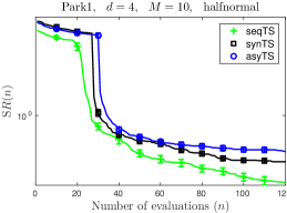
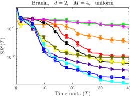
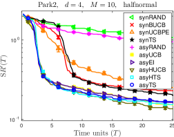
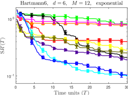
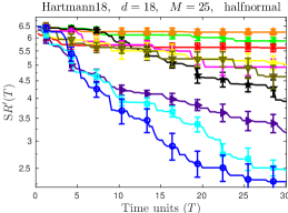
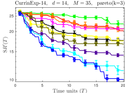
Figure 2: Results on the synthetic experiments. The title states the function used, its dimensionality $d$, the number of workers $M$ and the distribution used for the time. All distributions were constructed so that the expected time for one evaluation was one time unit. All figures were averaged over at least $15$ experiments.

The methods: We compare asyTS to the following. Synchronous Methods: synRAND: synchronous random sampling, synTS: synchronous TS, synBUCB from [8], synUCBPE from [7]. Aynchronous Methods: asyRAND: asynchronous random sampling, asyHUCB: an asynchronous version of UCB with hallucinated observations [8, 10], asyUCB: asynchronous upper confidence bound [36], asyEI: asynchronous expected improvement [19], asyHTS: asynchronous TS with hallucinated observations to explicitly encourage diversity. This last method is based on asyTS but bases the posterior on $\mathcal{D}_{j}\cup\{(x,\mu_{\mathcal{D}_{j}}(x))\}_{x\in F_{j}}$ in line 5 of Algorithm 2, where $F_{j}$ are the points in evaluation by other workers at step $j$ and $\mu_{\mathcal{D}_{j}}$ is the posterior mean conditioned on just $\mathcal{D}_{j}$; this preserves the mean of the GP, but shrinks the variance around the points in $F_{j}$. This method is inspired by [8, 10], who use such hallucinations for UCB/EI-type strategies so as to discourage picking points close to those that are already in evaluation. asyUCB and asyEI directly use the sequential UCB and EI criteria, since the the asynchronous versions do not repeatedly pick the same point for all workers. asyHUCB adds hallucinated observations to encourage diversity and is similar to [10] (who use EI instead) and can also be interpreted as an asynchronous version of [8]. While there are other methods for parallel BO, many of them are either computationally quite expensive and/or require tuning several hyperparameters. Furthermore, they are not straightforward to implement and their implementations are not publicly available. Appendix C describes additional implementation details for all BO methods.

Synthetic Experiments: We first present some results on a suite of benchmarks for global optimisation. To better align with our theoretical analysis, we add Gaussian noise to the function value when querying. This makes the problem more challenging that standard global optimisation where evaluations are not noisy. In our first experiment, we corroborate the claims in Theorem 1 by comparing the performance of seqTS, synTS, and asyTS in terms of the number of evaluations $n$ on the Park1 function. The results, displayed in the first panel of Fig. 2, confirm that when comparing solely in terms of $n$, the sequential version outperforms the parallel versions while the synchronous does marginally better than asynchronous.

Next, we present results on a series of global optimisation benchmarks with different values for the number of parallel workers $M$. We model the evaluation “time” as a random variable that is drawn from either a uniform, half-normal, exponential, or Pareto distribution. Each time a worker makes an evaluation, we also draw a sample from this time distribution and maintain a queueing data structure to simulate the different start and finish times for each evaluation. The results are presented in Fig. 2 where we plot the simple regret $\text{SR}^{\prime}(T)$ against (simulated) time $T$.

In the Park2 experiment, all asynchronous methods perform roughly the same and outperform the synchronous methods. On all other the other problems, asyTS performs best. asyHTS , which also uses hallucinated observations, performs about the same or slightly worse than asyTS, demonstrating that there is no need for encouraging diversity with TS. It is especially worth noting that the improvement of asyTS over other methods become larger as $M$ increases (e.g. $M>20$). We believe this ability to scale well with the number of workers is primarily due to the simplicity of our approach. In Appendix C, we provide these results in larger figures along with additional synthetic experiments.

Image Classification on Cifar-10: We also experiment with tuning hyperparameters of a $6$ layer convolutional neural network on an image classification task on the Cifar-10 dataset [25]. We tune the number of filters/neurons at each layer in the range $(16,256)$. Here, each function evaluation trains the model on 10K images for $20$ epochs and computes the validation accuracy on a validation set of 10K images. Our implementation uses Tensorflow [1] and we use a parallel set up of $M=4$ Titan X GPUs. The number of filters influences the training time which varied between $\sim 4$ to $\sim 16$ minutes depending on the size of the model. Note that this deviates from our theoretical analysis which treats function evaluation times as independent random variables, but it still introduces variability to evaluation times and demonstrates the robustness of our approach. Each method is given a budget of $2$ hours to find the best model by optimising accuracy on a validation set. These evaluations are noisy since the result of each training procedure depends on the initial parameters of the network and other stochasticity in the training procedure. Since the true value of this function is unknown, we simply report the best validation accuracy achieved by each method. Due to the expensive nature of this experiment we only compare $6$ of the above methods. The results are presented in Fig. 3. asyTS performs best on the validation accuracy. The following are ranges for the number of evaluations for each method over $9$ experiments; synchronous: synBUCB: 56 - 68, synTS: 56 - 68. asynchronous: asyRAND: 93 - 105, asyEI: 83 - 92, asyHUCB: 85 - 92, asyTS: 80 - 88.

While $20$ epochs is insufficient to completely train a model, the validation error gives a good indication of how well the model would perform after sufficient training. In Fig. 3, we also give the error on a test set of 10K images after training the best model chosen by each algorithm to completion, i.e. for $80$ epochs. asyTS and asyEI are able to recover the best models which achieve an accuracy of about $80\%$. While this falls short of state of the art results on Cifar-10 (for e.g. [13]), it is worth noting that we use only a small subset of the Cifar-10 dataset and a relatively small model. Nonetheless, it demonstrates the superiority of our approach over other baselines for hyperparameter tuning.

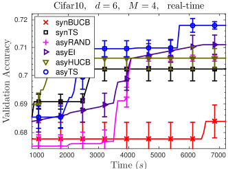
synBUCB	synTS	asyRAND
$74.37\pm 0.002$	$77.17\pm 1.01$	$76.07\pm 1.78$
asyEI	asyHUCB	asyTS
$\bf 80.51\pm 0.21$	$77.86\pm 1.12$	$\bf 80.47\pm 0.11$

Figure 3: Results on the Cifar-10 experiment. Left: The best validation set accuracy vs time for each method. Top: Test set accuracy after training the best model chosen by each method for $80$ epochs. The results presented are averaged over $9$ experiments.

5 Conclusion

This paper studies parallelised versions of TS for synchronous and asynchronous BO. We demonstrate that the algorithms synTS and asyTS perform as well as their purely sequential counterpart in terms of number of evaluations. However, when we factor time in, asyTS outperforms the other two versions. The main advantage of the proposed methods over existing literature is its simplicity, which enables us to scale well with a large number of workers.

We close with some intriguing avenues for future research. On a technical level, is the initialisation scheme of Proposition 2 necessary for TS? We are also interested in more general models for evaluation times, for example to capture correlations between the evaluation time and the query point $x_{j}\in\mathcal{X}$ that arise practice, such as in our CNN experiment. One could also consider models where some workers are slower than the rest. We look forward to pursuing these directions.

Appendix

Appendix A Theoretical Analysis for Parallelised Thompson Sampling in GPs

A.1 Some Relevant Results on GPs and GP Bandits

We first review some related results on GPs and GP bandits. We begin with the definition of the Maximum Information Gain (MIG) which characterises the statistical difficulty of GP bandits [36].

Definition 4 (Maximum Information Gain [36]).

Let $f\sim\mathcal{G}\mathcal{P}({\bf 0},\kappa)$ where $\kappa:\mathcal{X}^{2}\rightarrow\mathbb{R}$. Let $A=\{x_{1},\dots,x_{n}\}\subset\mathcal{X}$ be a finite subset. Let $f_{A},\epsilon_{A}\in\mathbb{R}^{n}$ such that $(f_{A})_{i}=f(x_{i})$ and $(\epsilon_{A})_{i}\sim\mathcal{N}(0,\eta^{2})$. Let $y_{A}=f_{A}+\epsilon_{A}\in\mathbb{R}^{n}$. Denote the Shannon Mutual Information by $I$. The MIG is the maximum information we can gain about $f$ using $n$ evaluations. That is,

$$\Psi_{n}=\max_{A\subset\mathcal{X},|A|=n}I(f;y_{A}).$$

Srinivas et al. [36] and Seeger et al. [33] provide bounds on the MIG for different classes of kernels. For example for the SE kernel, $\Psi_{n}\asymp\log(n)^{d+1}$ and for the Matérn kernel with smoothness parameter $\nu$, $\Psi_{n}\asymp n^{\frac{d(d+1)}{2\nu+d(d+1)}}\log(n)$. The next theorem due to Srinivas et al. [36] bounds the sum of variances of a GP using the MIG.

Lemma 5 (Lemma 5.2 and 5.3 in [36]).

Let $f\sim\mathcal{G}\mathcal{P}(0,\kappa)$, $f:\mathcal{X}\rightarrow\mathbb{R}$ and each time we query at any $x\in\mathcal{X}$ we observe $y=f(x)+\epsilon$, where $\epsilon\sim\mathcal{N}(0,\eta^{2})$. Let $\{x_{1},\dots,x_{n}\}$ be an arbitrary set of $n$ evaluations to $f$ where $x_{j}\in\mathcal{X}$ for all $j$. Let $\sigma^{2}_{j-1}$ denote the posterior variance conditioned on the first $j-1$ of these queries, $\{x_{1},\dots,x_{j-1}\}$. Then, $\sum_{j=1}^{n}\sigma^{2}_{j-1}(x_{j})\leq\frac{2}{\log(1+\eta^{-2})}\Psi_{n}$.

Next we will need the following regularity condition on the derivatives of the GP sample paths. When $f\sim\mathcal{G}\mathcal{P}({\bf 0},\kappa)$, it is satisfied when $\kappa$ is four times differentiable, e.g. the SE kernel and Matérn kernel when $\nu>2$ [9].

Assumption 6 (Gradients of GP Sample Paths [9]).

Let $f\sim\mathcal{G}\mathcal{P}({\bf 0},\kappa)$, where $\kappa:\mathcal{X}^{2}\rightarrow\mathbb{R}$ is a stationary kernel. The partial derivatives of $f$ satisfies the following condition. There exist constants $a,b>0$ such that,

$$\text{for all $J>0$, $\;$and for all $i\in\{1,\dots,d\}$},\quad\mathbb{P}\left(\sup_{x}\Big{|}\frac{\partial f(x)}{\partial x_{i}}\Big{|}>J\right)\leq ae^{-(J/b)^{2}}.$$

Finally, we will need the following result on the supremum of a Gaussian process. It is satisfied when $\kappa$ is twice differentiable.

Lemma 7 (Supremum of a GP [2]).

Let $f\sim\mathcal{G}\mathcal{P}(0,\kappa)$ have continuous sample paths. Then, $\mathbb{E}\|f\|_{\infty}=\,\Xi\,<\infty$.

This, in particular implies that in the definition of ${\text{BSR}^{\prime}}({T})$ in (3), $\max_{x\in\mathcal{X}}|f(x_{\star})-f(x)|\leq 2\,\Xi\,$.

Finally, we will use the following result in our parallel analysis. Recall that the posterior variance of a GP does not depend on the observations.

Lemma 8 (Lemma 1 (modified) in [8]).

Let $f\sim\mathcal{G}\mathcal{P}(0,\kappa)$. Let $A,B$ be finite subsets of $\mathcal{X}$. Let $y_{A}\in\mathbb{R}^{|A|}$ and $y_{B}\in\mathbb{R}^{|B|}$ denote the observations when we evaluate $f$ at $A$ and $B$ respectively. Further let $\sigma_{A},\,\sigma_{A\cup B}\,:\,\mathcal{X}\rightarrow\mathbb{R}$ denote the posterior standard deviation of the GP when conditioned on $A$ and $A\cup B$ respectively. Then,

$$\text{for all $x\in\mathcal{X}$},\hskip 14.45377pt\frac{\sigma_{A}(x)}{\sigma_{A\cup B}(x)}\leq\exp\big{(}I(f;y_{B}|y_{A})\big{)}$$

The proof exactly mimics the proof in Desautels et al. [8]. Lemma 8 implies $\sigma_{A}(x)\leq\xi_{M}^{1/2}\sigma_{A\cup B}(x)$ where $\xi_{M}$ is from (4).

A.2 Notation & Set up

We will require some set up in order to unify the analysis for the sequential, synchronously parallel and asynchronously parallel settings.

• The first is an indexing for the function evaluations. This is illustrated for the synchronous and asynchronous parallel settings in Figure 1. In our analysis, the index $j$ or step $j$ will refer to the $j$${}^{\textrm{th}}$ function evaluation dispatched by the algorithm. In the sequential setting this simply means that there were $j-1$ evaluations before the $j$${}^{\textrm{th}}$ . For synchronous strategies we index the first batch from $j=1,\dots,M$ and then the next batch $j=M+1,\dots,2M$ and so on as in Figure 1. For the asynchronous setting, this might differ as each evaluation takes different amounts of time. For example, in Figure 1, the first worker finishes the $j=1$${}^{\textrm{st}}$ job and then starts the $j=4$${}^{\textrm{th}}$, while the second worker finishes the $j=2$${}^{\textrm{nd}}$ job and starts the $j=6$${}^{\textrm{th}}$.

• Next, we define $\mathcal{D}_{j}$ at step $j$ of the algorithm to be the query-observation pairs $(x_{k},y_{k})$ for function evaluations completed by step $j$. In the sequential setting $\mathcal{D}_{j}=\{(x_{k},y_{k}):k\in\{1,\dots,j-1\}\}$ for all $j$. For the synchronous setting in Figure 1, $\mathcal{D}_{1}=\mathcal{D}_{2}=\mathcal{D}_{3}=\varnothing$, $\mathcal{D}_{4}=\mathcal{D}_{5}=\mathcal{D}_{6}=\{(x_{k},y_{k}):k\in\{1,2,3\}\}$, $\mathcal{D}_{7}=\mathcal{D}_{8}=\mathcal{D}_{9}=\{(x_{k},y_{k}):k\in\{1,2,3,4,5,6\}\}$ etc. Similarly, for the asynchronous setting, $\mathcal{D}_{1}=\mathcal{D}_{2}=\mathcal{D}_{3}=\varnothing$, $\mathcal{D}_{4}=\{(x_{k},y_{k}):k\in\{1\}\}$, $\mathcal{D}_{5}=\{(x_{k},y_{k}):k\in\{1,3\}\}$, $\mathcal{D}_{6}=\{(x_{k},y_{k}):k\in\{1,2,3\}\}$, $\mathcal{D}_{7}=\{(x_{k},y_{k}):k\in\{1,2,3,5\}\}$ etc. Note that in the asynchronous setting $|\mathcal{D}_{j}|=j-M$ for all $j>M$. $\{\mathcal{D}_{j}\}_{j\geq 1}$ determines the filtration when constructing the posterior GP at every step $j$.

• Finally, in all three settings, $\mu_{A}:\mathcal{X}\rightarrow\mathbb{R}$ and $\sigma_{A}:\mathcal{X}\rightarrow\mathbb{R}_{+}$ will refer to the posterior mean and standard deviation of the GP conditioned on some evaluations $A$, i.e. $A\subset\mathcal{X}\times\mathbb{R}$ is a set of $(x,y)$ values and $|A|<\infty$. They can be computed by plugging in the $(x,y)$ values in $A$ to (1). For example, $\mu_{\mathcal{D}_{j}},\sigma_{\mathcal{D}_{j}}$ will denote the mean and standard deviation conditioned on the completed evaluations, $\mathcal{D}_{j}$. Finally, when using our indexing scheme above we will also overload notation so that $\sigma_{j-1}$ will denote the posterior standard deviation conditioned on evaluations from steps $1$ to $j-1$. That is $\sigma_{j-1}=\sigma_{A}$ where $A=\{(x_{k},y_{k})\}_{k=1}^{j-1}$.

A.3 Parallelised Thompson Sampling

In the remainder of this section, $\beta_{n}\in\mathbb{R}$ for all $n\geq 1$ will denote the following value.

$$\beta_{n}\,=\,4(d+1)\log(n)+2d\log(dab\sqrt{\pi})\;\;\asymp\;d\log(n),$$ (5)

Here $d$ is the dimension, $a,b$ are from Assumption 6, and $n$ will denote the number of evaluations. Our first theorem below is a bound on the simple regret for synTS and asyTS after $n$ completed evaluations.

Theorem 9.

Let $f\sim\mathcal{G}\mathcal{P}({\bf 0},\kappa)$ where $\kappa:\mathcal{X}^{2}\rightarrow\mathbb{R}$ satisfies Assumption 6. Further, without loss of generality $\kappa(x,x^{\prime})\leq 1$. Then for synTS and asyTS, the Bayes simple regret after $n$ evaluations satisfies,

$${\text{BSR}}({n})\;\leq\;\frac{C_{1}}{n}+\sqrt{\frac{C_{2}\xi_{M}\beta_{n}\Psi_{n}}{n}},$$

where $\Psi_{n}$ is the MIG in Definition 4, $\beta_{n}$ is as defined in (5), $\xi_{M}$ is from (4), and $C_{1}=\pi^{2}/6+\sqrt{2\pi}/12$, $\;C_{2}=2/\log(1+\eta^{-2})$ are constants.

Proof.

Our proof is based on techniques from Russo and Van Roy [31] and Srinivas et al. [36]. We will first assume that the $n$ evaluations completed are the the evaluations indexed $j=1,\dots,n$.

As part of analysis, we will discretise $\mathcal{X}$ at each step $j$ of the algorithm. Our discretisation $\nu_{j}$, is obtained via a grid of $\tau_{j}=j^{2}dab\sqrt{\pi}$ equally spaced points along each coordinate and has size $|\nu_{j}|=\tau_{j}^{d}$. It is easy to verify that $\nu_{j}$ satisfies the following property: for all $x\in\mathcal{X}$, $\|x-[x]_{j}\|_{1}\leq d/\tau_{j}$, where $[x]_{j}$ is the closest point to $x$ in $\nu_{j}$. This discretisation is deterministically constructed ahead of time and does not depend on any of the random quantities in the problem.

For the purposes of our analysis, we define the Bayes cumulative regret after $n$ evaluations as,

$$\text{BCR}({n})=\mathbb{E}\bigg{[}\sum_{j=1}^{n}f(x_{\star})-f(x_{j})\bigg{]}.$$

Here, just as in (2), the expectation is with respect to the randomness in the prior, observations and algorithm. Since the average is larger than the minimum, we have $\frac{1}{n}\sum_{j}f(x_{\star})-f(x_{j})\geq\min_{j}(f(x_{\star})-f(x_{j}))=\text{SR}(n)$; hence ${\text{BSR}}({n})\leq\frac{1}{n}\text{BCR}({n})$.

Following Russo and Van Roy [31] we denote $U_{j}(\cdot)=\mu_{\mathcal{D}_{j}}(\cdot)+\beta^{1/2}_{j}\sigma_{\mathcal{D}_{j}}(\cdot)$ to be an upper confidence bound for $f$ and begin by decomposing $\text{BCR}({n})$ as follows,

$$\text{BCR}({n})\; =\;\sum_{j=1}^{n}\mathbb{E}\left[f(x_{\star})-f(x_{j})\right]\stackrel{{\scriptstyle(a)}}{{=}}\;\sum_{j=1}^{n}\mathbb{E}\big{[}\mathbb{E}\left[f(x_{\star})-f(x_{j})\,|\mathcal{D}_{j}\right]\,\big{]}$$

$$\stackrel{{\scriptstyle(b)}}{{=}}\;\sum_{j=1}^{n}\mathbb{E}\big{[}\mathbb{E}[f(x_{\star})-f(x_{j})-f([x_{\star}]_{j})+f([x_{\star}]_{j})-U_{j}([x_{\star}]_{j})+U_{j}([x_{j}]_{j})\,-$$

$$\hskip 216.81ptf([x_{j}]_{j})+f([x_{j}]_{j})-f(x_{j})\,|\mathcal{D}_{j}]\,\big{]}$$

$$\stackrel{{\scriptstyle(c)}}{{=}}\;\underbrace{\sum_{j=1}^{n}\mathbb{E}[f(x_{\star})-f([x_{\star}]_{j})]}_{A_{1}}\;+\;\underbrace{\sum_{j=1}^{n}\mathbb{E}[f([x_{j}]_{j})-f(x_{j})]}_{A_{2}}\;+\;\underbrace{\sum_{j=1}^{n}\mathbb{E}[f([x_{\star}]_{j})-U_{j}([x_{\star}]_{j})]}_{A_{3}}$$

$$\hskip 144.54pt\;+\;\underbrace{\sum_{j=1}^{n}\mathbb{E}[U_{j}([x_{j}]_{j})-f([x_{j}]_{j})]}_{A_{4}}.$$

In $(a)$ we have used the tower property of expectation and in $(c)$ we have simply rearranged the terms from the previous step. In $(b)$ we have added and subtracted $f([x_{\star}]_{j})$ and then $f([x_{j}]_{j})$. The crucial step in $(b)$ is that we have also added $-U_{j}([x_{\star}]_{j})+U_{j}([x_{j}]_{j})$ which is justified if $\mathbb{E}[U_{j}([x_{\star}]_{j})|\mathcal{D}_{j}]=\mathbb{E}[U_{j}([x_{j}]_{j})|\mathcal{D}_{j}]$. For this, first note that as $x_{j}$ is sampled from the posterior distribution for $x_{\star}$ conditioned on $\mathcal{D}_{j}$, both $x_{j}|\mathcal{D}_{j}$ and $x_{\star}|\mathcal{D}_{j}$ have the same distribution. Since the discretisation $\nu_{j}$ is fixed ahead of time, and $U_{j}$ is deterministic conditioned on $\mathcal{D}_{j}$, so do $U_{j}([x_{j}]_{j})|\mathcal{D}_{j}$ and $U_{j}([x_{\star}]_{j})|\mathcal{D}_{j}$. Therefore, both quantities are also equal in expectation.

To bound $A_{1},A_{2}$ and $A_{3}$ we use the following Lemmas. The proofs are in Sections A.3.1 and A.3.2.

Lemma 10.

At step $j$, for all $x\in\mathcal{X}$, $\mathbb{E}[|f(x)-f([x]_{j})|]\leq\frac{1}{2j^{2}}$.

Lemma 11.

At step $j$, for all $x\in\nu_{j}$, $\mathbb{E}[\mathbbm{1}\{f(x)>U_{j}(x)\}\cdot(f(x)-U_{j}(x))]\leq\frac{1}{j^{2}\sqrt{2\pi}|\nu_{j}|}$.

Using Lemma 10 and the fact that $\sum_{j}j^{-2}=\pi^{2}/6$, we have $A_{1}+A_{2}\leq\pi^{2}/6$. We bound $A_{3}$ via,

$$A_{3}\; \leq\;\mathbb{E}\bigg{[}\sum_{j=1}^{n}\mathbbm{1}\{f([x_{\star}]_{j})>U_{j}([x_{\star}]_{j})\}\cdot(f([x_{\star}]_{j})-U_{j}([x_{\star}]_{j}))\bigg{]}$$

$$\leq\;\sum_{j=1}^{n}\sum_{x\in\nu_{j}}\mathbb{E}\big{[}\,\mathbbm{1}\{f(x)>U_{j}(x)\}\cdot(f(x)-U_{j}(x))\,\big{]}\leq\;\sum_{j=1}^{n}\sum_{x\in\nu_{j}}\frac{1}{j^{2}\sqrt{2\pi}|\nu_{j}|}=\frac{\sqrt{2\pi}}{12}$$

In the first step we upper bounded $A_{3}$ by only considering the positive terms in the summation. The second step bounds the term for $[x_{\star}]_{j}$ by the sum of corresponding terms for all $x\in\nu_{j}$. We then apply Lemma 11.

Finally, we bound each term inside the summation of $A_{4}$ as follows,

$$\mathbb{E}[U_{j}([x_{j}]_{j})-f([x_{j}]_{j})]=\mathbb{E}[\mu_{\mathcal{D}_{j}}([x_{j}]_{j})+\beta^{1/2}_{j}\sigma_{\mathcal{D}_{j}}([x_{j}]_{j})-f([x_{j}]_{j})]$$ (6)

$$\hskip 28.90755pt=\mathbb{E}[\mu_{\mathcal{D}_{j}}([x_{j}]_{j})+\beta^{1/2}_{j}\sigma_{\mathcal{D}_{j}}([x_{j}]_{j})-\mathbb{E}[f([x_{j}]_{j})|\mathcal{D}_{j}]]=\mathbb{E}[\beta^{1/2}_{j}\sigma_{\mathcal{D}_{j}}([x_{j}]_{j})]$$

Once again, we have used the fact that $\mu_{\mathcal{D}_{j}},\sigma_{\mathcal{D}_{j}}$ are deterministic given $\mathcal{D}_{j}$. Therefore,

$$A_{4} \stackrel{{\scriptstyle(a)}}{{\leq}}\beta^{1/2}_{n}\sum_{j=1}^{n}\mathbb{E}[\sigma_{\mathcal{D}_{j}}([x_{j}]_{j})]\stackrel{{\scriptstyle(b)}}{{\leq}}\beta^{1/2}_{n}\xi_{M}^{1/2}\mathbb{E}\Bigg{[}\sum_{j=1}^{n}\sigma_{j-1}([x_{j}]_{j})\Bigg{]}$$

$$\stackrel{{\scriptstyle(c)}}{{\leq}}\beta^{1/2}_{n}\xi_{M}^{1/2}\mathbb{E}\Bigg{[}\bigg{(}n\sum_{j=1}^{n}\sigma^{2}_{j}([x_{j}]_{j})\bigg{)}^{1/2}\Bigg{]}\stackrel{{\scriptstyle(d)}}{{\leq}}\sqrt{\frac{2\xi_{M}n\beta_{n}\Psi_{n}}{\log(1+\eta^{-2})}}$$ (7)

Here, $(a)$ uses (6) and that $\beta_{j}$ is increasing in $j$ (5). $(c)$ uses the Cauchy-Schwarz inequality and $(d)$ uses Lemma 5. For $(b)$, first we note that $\mathcal{D}_{j}\subseteq\{(x^{(i)},y^{(i)})\}_{i=1}^{j-1}$. In the synchronously parallel setting $\mathcal{D}_{j}$ could be missing up to $M$ of these $j-1$ evaluations, i.e. $|\mathcal{D}_{j}|=\lfloor(j-1)/M\rfloor$. In the asynchronous setting we will be missing exactly $M$ evaluations except during the first $M$ steps, i.e. $|\mathcal{D}_{j}|=j-M$ for all $j>M$. In either case, letting $A=\mathcal{D}_{j}$ and $B=\{(x^{(i)},y^{(i)})\}_{i=1}^{j-1}\backslash\mathcal{D}_{j}$ in Lemma 8 we get,

$$\text{for all $x\in\mathcal{X}$},\hskip 14.45377pt\sigma_{\mathcal{D}_{j}}(x)\,\leq\,\exp\big{(}I(f;y_{B}|y_{\mathcal{D}_{j}})\big{)}\,\sigma_{j-1}(x)\,\leq\,\xi_{M}^{1/2}\sigma_{j-1}(x).$$ (8)

The last step uses (4) and that $|B|<M$. Putting the bounds for $A_{1},A_{2},A_{3}$, and $A_{4}$ together we get, $\text{BCR}({n})\;\leq\;C_{1}+\sqrt{C_{2}n\beta_{n}\Psi_{n}}$. The theorem follows from the relation ${\text{BSR}}({n})\leq\frac{1}{n}\text{BCR}({n})$.

Finally consider the case where the $n$ evaluations completed are not the first $n$ dispatched. Since $A_{1},A_{2},A_{3}$ are bounded by constants summing over all $n$ we only need to worry about $A_{4}$. In step $(a)$ of (7), we have bounded $A_{4}$ by the sum of posterior variances $\sigma_{\mathcal{D}_{j}}([x_{j}]_{j})$. Since $\sigma_{\mathcal{D}_{j^{\prime}}}([x_{j}]_{j})<\sigma_{\mathcal{D}_{j}}([x_{j}]_{j})$ for $j^{\prime}>j$, the sum for any $n$ completed evaluations can be bound by the same sum for the first $n$ evaluations dispatched. The result follows accordingly. ∎

The bound for the sequential setting in Theorem 1 follows directly by setting $M=1$ in the above analysis.

Corollary 12.

Assume the same setting and quantities as in Theorem 9. Then for seqTS, the Bayes’ simple regret after $n$ evaluations satisfies,

$${\text{BSR}}({n})\;\leq\;\frac{C_{1}}{n}+\sqrt{\frac{C_{2}\beta_{n}\Psi_{n}}{n}},$$

Proof.

The proof follows on exactly the same lines as above. The only difference is that we will not require step $(b)$ in (7) and hence will not need $\xi_{M}$. ∎

We conclude this section with justification for the discussion following Theorem 1. Precisely that $B^{\text{{seq}}}_{n}\leq B^{\text{{syn}}}_{n}\leq B^{\text{{asy}}}_{n}$ where $B^{\text{{seq}}}_{n},B^{\text{{syn}}}_{n},B^{\text{{asy}}}_{n}$ refer to the best achievable upper bounds using our analysis. We first note that in Lemma 8, $\sigma_{A\cup B}\leq\sigma_{A}$ as the addition of more points can only decrease the posterior variance. Therefore, $\xi_{M}$ is necessarily larger than $1$. Hence $B^{\text{{seq}}}_{n}\leq B^{\text{{syn}}}_{n},B^{\text{{asy}}}_{n}$. The result $B^{\text{{syn}}}_{n}\leq B^{\text{{asy}}}_{n}$ can be obtained by a more careful analysis. Precisely, in (7) and (8) we will have to use $\xi_{M}$ for the asynchronous setting for all $j>M$ since $|B|=|\{(x^{(i)},y^{(i)})\}_{i=1}^{j-1}\backslash\mathcal{D}_{j}|=M$. However, in the synchronous setting we can use a bound $\xi_{|B|}$ where $|B|$ is less than $M$ most of the time. Of course, the difference of $B^{\text{{syn}}}_{n},B^{\text{{asy}}}_{n}$ relative to the $B^{\text{{seq}}}_{n}$ is dominated by the maximum number of missing evaluations which is $M-1$ for both synTS and asyTS. We reiterate that $B^{\text{{seq}}}_{n},B^{\text{{syn}}}_{n},B^{\text{{asy}}}_{n}$ are upper bounds on the Bayes’ regret ${\text{BSR}}({n})$ and not the actual regret itself.

A.3.1 Proof of Lemma 10

Let $L=\sup_{i=1,\dots,d}\sup_{x\in\mathcal{X}}\big{|}\frac{\partial f(x)}{\partial x_{i}}\big{|}$. By Assumption 6 and the union bound we have $\mathbb{P}(L\geq t)\leq da\exp^{-t^{2}/b^{2}}$. Let $x\in\mathcal{X}$. We bound,

$$\mathbb{E}[|f(x)-f([x]_{j})|] \leq\mathbb{E}[L\|x-[x]_{j}\|_{1}]\leq\frac{d}{\tau_{j}}\mathbb{E}[L]=\frac{d}{\tau_{j}}\int_{0}^{\infty}\mathbb{P}(L\geq t)\mathrm{d}t$$

$$\leq\frac{d}{\tau_{j}}\int_{0}^{\infty}ae^{t^{2}/b^{2}}\mathrm{d}t=\frac{dab\sqrt{\pi}}{2\tau_{j}}=\frac{1}{2j^{2}}.$$

The first step bounds the difference in the function values by the largest partial derivative and the $L^{1}$ distance between the points. The second step uses the properties of the discretisation $\nu_{j}$ and the third step uses the identity $\mathbb{E}X=\int\mathbb{P}(X>t)\mathrm{d}t$ for positive random variables $X$. The last step uses the value for $\tau_{j}$ specified in the main proof. ∎

A.3.2 Proof of Lemma 11

The proof is similar to Lemma 2 in [31], but we provide it here for completeness. We will use the fact that for $Z\sim\mathcal{N}(\mu,\sigma^{2})$, we have $\mathbb{E}[Z\mathbbm{1}(Z>0)]=\frac{\sigma}{\sqrt{2\pi}}e^{-\mu^{2}/(2\sigma^{2})}$. Noting that $f(x)-U_{j}(x)|\mathcal{D}_{j}\sim\mathcal{N}(-\beta^{1/2}_{j}\sigma_{\mathcal{D}_{j}}(x),\sigma^{2}_{\mathcal{D}_{j}}(x))$, we have,

$$\mathbb{E}[\mathbbm{1}\{f(x)>U_{j}(x)\}\cdot(f(x)-U_{j}(x))|\mathcal{D}_{j}]=\frac{\sigma_{\mathcal{D}_{j}}(x)}{\sqrt{2\pi}}e^{\beta_{j}/2}\leq\frac{1}{\sqrt{2\pi}|\nu_{j}|j^{2}}.$$

Here, the last step uses that $\sigma_{\mathcal{D}_{j}}(x)\leq\kappa(x,x)\leq 1$ and that $\beta_{j}=2\log(j^{2}|\nu_{j}|)$. ∎

A.4 On the Initialisation Scheme and Subsequent Results – Proposition 2

The bound $\xi_{M}$ could be quite large growing as fast as $M$, which is very unsatisfying because then the bounds are no better than a strictly sequential algorithm for $n/M$ evaluations.  Desautels et al. [8] show however that $\xi_{M}$ can be bounded by a constant $C^{\prime}$ if we bootstrap a procedure with an uncertainty sampling procedure. Precisely, we pick $x^{\text{init}}_{1}=\mathop{\mathrm{argmax}}_{x\in\mathcal{X}}\sigma^{2}_{0}(x)$ where $\sigma^{2}_{0}$ is the prior variance; We then iterate $x^{\text{init}}_{j}=\mathop{\mathrm{argmax}}_{x\in\mathcal{X}}\sigma^{2}_{j-1}(x)$ until $j=n_{\text{init}}$. As the posterior variance of a GP does not depend on the evaluations, this scheme is asynchronously parallelisable: simply pre-compute the $n_{\text{init}}$ evaluation points and then deploy them in parallel.

By using the same initialisation scheme, we can achieve, for both synTS and asyTS, the following:

$${\text{BSR}}({n})\;\leq\;C^{\prime}B^{\text{{seq}}}_{n}\,+\,\frac{2\,\Xi\,n_{\text{init}}}{n}$$

Here, $B^{\text{{seq}}}_{n}$ is the simple regret of seqTS. The proof simply replaces the unconditional mutual information in the definition of the MIG with the mutual information conditioned on the first $n_{\text{init}}$ evaluations. Desautels et al. [8] provide bounds for $C^{\prime}$ for different kernels. For the SE kernel, $C^{\prime}=\exp((2d/e)^{d})$ and for the Matérn kernel $C^{\prime}=e$. They also show that $n_{\text{init}}$ typically scales as $\mathcal{O}(M{\bf{\rm polylog}}(M))$. If $M$ does not grow too large with $n$, then the first term above dominates and we are worse than the sequential bound only up to constant factors.

In practice however, as we have alluded to already in the main text, there are two shortcomings with this initialisation scheme. First, it requires that we know the kernel before any evaluations to $f$. Most BO procedures tune the kernel on the fly using its past evaluations, but this is problematic without any evaluations. Second the size of the initialisation set $n_{\text{init}}$ has some problem dependent constants that we will not have access to in practice. We conjecture that TS will not need this initialisation and wish to resolve this in future work.

Appendix B Proofs for Parallelised Thompson Sampling with Random Evaluation Times

The goal of this section is to prove Theorem 3. In Section B.2 we derive some concentration results for uniform and half-normal distributes and their maxima. In Section B.3 we do the same for exponential random variables. We put everything together in Section B.4 to prove Theorem 3. We begin by reviewing some well known concepts in concentration of measure.

B.1 Some Relevant Results

We first introduce the notion of sub-Gaussianity, which characterises one of the stronger types of tail behaviour for random variables.

Definition 13 (Sub-Gaussian Random Variables).

A zero mean random variable is said to be $\tau$ sub-Gaussian if it satisfies, $\mathbb{E}[e^{\lambda X}]\;\leq\;e^{\frac{\tau^{2}\lambda^{2}}{2}}$ for all $\lambda\in\mathbb{R}$.

It is well known that Normal $\mathcal{N}(0,\zeta^{2})$ variables are $\zeta$ sub-Gaussian and bounded random variables with support in $[a,b]$ are $(b-a)/2$ sub-Gaussian. For sub-Gaussian random variables, we have the following important and well known result.

Lemma 14 (Sub-Gaussian Tail Bound).

Let $X_{1},\dots,X_{n}$ be zero mean independent random variables such that $X_{i}$ is $\sigma_{i}$ sub-Gaussian. Denote $S_{n}=\sum_{i=1}^{n}X_{i}$ and $\sigma^{2}=\sum_{i=1}^{n}\sigma_{i}^{2}$. Then, for all $\epsilon>0$,

$$\mathbb{P}\left(S_{n}\geq\epsilon\right)\;\leq\;\exp\left(\frac{-\epsilon^{2}}{2\sigma^{2}}\right),\hskip 14.45377pt\mathbb{P}\left(S_{n}\leq\epsilon\right)\;\leq\;\exp\left(\frac{-\epsilon^{2}}{2\sigma^{2}}\right).$$

We will need the following result for Lipschitz functions of Gaussian random variables in our analysis of the half-normal distribution for time, see Theorem 5.6 in Boucheron et al. [5].

Lemma 15 (Gaussian Lipschitz Concentration [5]).

Let $X\in\mathbb{R}^{n}$ such that $X_{i}\sim\mathcal{N}(0,\zeta^{2})$ iid for $i=1,\dots,n$. Let $F:\mathbb{R}^{n}\rightarrow\mathbb{R}$ be an $L$-Lipschitz function, i.e. $|F(x)-F(y)|\leq L\|x-y\|_{2}$ for all $x,y\in\mathbb{R}^{n}$. Then, for all $\lambda>0$, $\mathbb{E}[\exp^{\lambda F(X)}]\leq\exp\left(\frac{\pi^{2}L^{2}\zeta^{2}}{8}\lambda^{2}\right)$. That is, $F(X)$ is $\frac{\pi L\zeta}{2}$ sub-Gaussian.

We also introduce Sub-Exponential random variables, which have a different tail behavior.

Definition 16 (Sub-Exponential Random Variables).

A zero mean random variable is said to be sub-Exponential with parameters $(\tau^{2},b)$ if it satisfies, $\mathbb{E}[e^{\lambda X}]\;\leq\;e^{\frac{\tau^{2}\lambda^{2}}{2}}$ for all $\lambda$ with $|\lambda|\leq 1/b$.

Sub-Exponential random variables are a special case of Sub-Gamma random variables (See Chapter 2.4 in Boucheron et al. [5]) and allow for a Bernstein-type inequality.

Proposition 17 (Sub-Exponential tail bound [5]).

Let $X_{1},\dots,X_{n}$ be independent sub-exponential random variables with parameters $(\sigma_{i}^{2},b_{i})$. Denote $S_{n}=\sum_{i=1}^{n}X_{i}$ and $\sigma^{2}=\sum_{i=1}^{n}\sigma_{i}^{2}$ and $b=\max_{i}b_{i}$. Then, for all $\epsilon>0$,

$$\mathbb{P}\left(\Big{|}S_{n}-\sum_{i=1}^{n}\mu_{i}\Big{|}\geq\sqrt{2\sigma^{2}t}+bt\right)\leq 2\exp(-t).$$

B.2 Results for Uniform and Half-normal Random Variables

In the next two lemmas, let $\{X_{i}\}_{i=1}^{M}$ denote a sequence of $M$ i.i.d random variables and $Y=\max_{i}X_{i}$ be their maximum. We note that the results or techniques in Lemmas 18, 19 are not particularly new.

Lemma 18.

Let $X_{i}\sim\text{Unif}(a,b)$. Then $\mathbb{E}X_{i}=\theta$ and $\mathbb{E}Y=\theta+\frac{M-1}{M+1}\frac{b-a}{2}$ where $\theta=(a+b)/2$.

Proof.

The proof for $\mathbb{E}X_{i}$ is straightforward. The cdf of $Y$ is $\mathbb{P}(Y\leq t)=\prod_{i=1}^{M}\mathbb{P}(X_{i}\leq t)=(\frac{t-a}{b-a})^{M}$. Therefore its pdf is $p_{Y}(t)=M(t-a)^{M-1}/(b-a)^{M}$ and its expectation is

$$\mathbb{E}[Y]=\int_{a}^{b}tM(t-a)^{M-1}/(b-a)^{M}\mathrm{d}t=\frac{a+bM}{M+1}=\theta+\frac{M-1}{M+1}\frac{b-a}{2}.$$

∎

Lemma 19.

Let $X_{i}\sim\mathcal{H}\mathcal{N}(\zeta^{2})$. Then $\mathbb{E}X_{i}=\zeta\sqrt{2/\pi}$ and $\mathbb{E}Y$ satisfies,

$$\zeta K\sqrt{\log(M)}\leq\mathbb{E}Y\leq\zeta\sqrt{2\log(2M)}.$$

Here $K$ is a universal constant. Therefore, $\mathbb{E}Y\in\Theta(\sqrt{\log(M)})\mathbb{E}X_{i}$.

Proof.

The proof for $\mathbb{E}X_{i}$ just uses integration over the pdf $p_{Y}(t)=\frac{\sqrt{2}}{\sqrt{\pi\zeta^{2}}}e^{-\frac{t^{2}}{2\sigma^{2}}}$. For the second part, writing the pdf of $\mathcal{N}(0,\zeta^{2})$ as $\phi(t)$ we have,

$$\mathbb{E}[e^{\lambda X_{i}}]=2\int_{0}^{\infty}e^{\lambda t}\phi(t)\mathrm{d}t\leq 2\int_{-\infty}^{\infty}e^{\lambda t}\phi(t)\mathrm{d}t=2\mathbb{E}_{Z\sim\mathcal{N}(0,\zeta^{2})}[e^{\lambda Z}]=2e^{\zeta^{2}\lambda^{2}/2}.$$

The inequality in the second step uses that the integrand is positive. Therefore, using Jensen’s inequality and the fact that the maximum is smaller than the sum we get,

$$e^{\lambda\mathbb{E}[Y]}\leq\mathbb{E}[e^{\lambda Y}]\leq\sum_{i=1}^{n}\mathbb{E}[e^{\lambda X_{i}}]\leq 2Me^{\lambda^{2}\zeta^{2}/2}\hskip 7.22743pt\implies\hskip 7.22743pt\mathbb{E}[Y]\leq\frac{1}{\lambda}\log(2M)+\frac{\zeta^{2}\lambda}{2}.$$

Choosing $\lambda=\frac{\sqrt{2\log(2M)}}{\zeta}$ yields the upper bound. The lower bound follows from Lemma 4.10 of Adler [2] which establishes a $K\sqrt{\log(M)}$ lower bound for $M$ i.i.d standard normals $Z_{1},\dots,Z_{M}$. We can use the same lower bound since $|Z_{i}|\geq Z_{i}$. ∎

Lemma 20.

Suppose we complete a sequence of jobs indexed $j=1,2,\dots$. The time taken for the jobs $\{X_{j}\}_{j\geq 1}$ are i.i.d with mean $\theta$ and sub-Gaussian parameter $\tau$. Let $\delta\in(0,1)$, and $N$ denote the number of completed jobs after time $T$. That is, $N$ is the random variable such that $N=\max\{n\geq 1;\sum_{j=1}^{n}X_{j}\leq T\}$. Then, with probability greater than $1-\delta$, for all $\alpha\in(0,1)$, there exists $T_{\alpha,\delta}$ such that for all $T>T_{\alpha,\delta}$, $N\in\Big{(}\frac{T}{\theta(1+\alpha)}-1,\frac{T}{\theta(1-\alpha)}\Big{)}$.

Proof.

We will first consider the total time taken $S_{n}=\sum_{i=1}^{n}X_{i}$ after $n$ evaluations. Let $\epsilon_{n}=\tau\sqrt{n\log(n^{2}\pi^{2}/(3\delta))}$ throughout this proof. Using Lemma 14, we have $\mathbb{P}(|S_{n}-n\theta|>\epsilon_{n})=6\delta/(n\pi^{2})$. By a union bound over all $n\geq 1$, we have that with with probability greater than $\delta$, the following event $\mathcal{E}$ holds.

$$\mathcal{E}=\{\forall n\geq 1,\;\;|S_{n}-n\theta|\leq\epsilon_{n}.\}$$ (9)

Since $\mathcal{E}$ is a statement about all time steps, it is also for true the random number of completed jobs $N$. Inverting the condition in (9) and using the definition of $N$, we have

$$N\theta-\epsilon_{N}\leq S_{N}\leq T\leq S_{N+1}\leq(N+1)\theta+\epsilon_{N+1}.$$ (10)

Now assume that there exists $T_{\alpha,\delta}$ such that for all $T\geq T_{\alpha,\delta}$ we have, $\epsilon_{N}\leq N\alpha\theta$. Since $\epsilon_{n}$ is sub-linear in $n$, it also follows that $\epsilon_{N+1}\leq(N+1)\alpha\theta$. Hence, $N\theta(1-\alpha)\leq T\leq(N+1)\theta(1+\alpha)$ and the result follows.

All that is left to do is to establish that such a $T_{\alpha,\delta}$ exists under event $\mathcal{E}$, for which we will once again appeal to (10). The main intuition is that as $\epsilon_{N}\asymp\sqrt{N\log(N)}$, the condition $\epsilon_{N}\leq N\alpha\theta$ is satisfied for $N$ large enough. But $N$ is growing with $T$, and hence it is satisfied for $T$ large enough. More formally, since $\frac{N}{\epsilon_{N}}\asymp\frac{N+1}{\epsilon_{N+1}}$ using the upper bound for $T$ it is sufficient to show $\frac{T}{\epsilon_{N+1}}\gtrsim\frac{1}{\alpha\theta}$ for all $T\geq T_{\alpha,\delta}$. But since $\epsilon_{N+1}\asymp\sqrt{N\log(N)}$ and the lower bound for $T$ is $T\gtrsim N$, it is sufficient if $\frac{T}{\sqrt{T\log(T)}}\gtrsim\frac{1}{\alpha\theta}$ for all $T\geq T_{\alpha,\delta}$. This is achievable as the LHS is increasing with $T$ and the RHS is constant. ∎

Our final result for the uniform and half-normal random variables follows as a consequence of Lemma 20.

Theorem 21.

Let the time taken $X$ for completing an evaluation to $f$ be a random variable.

• If $X\sim\textrm{Unif}(a,b)$, denote $\theta=(a+b)/2$, $\,\theta_{M}=\theta+\frac{M-1}{M+1}\frac{b-a}{2}$, and $\tau=(b-a)/2$.

• If $X\sim\mathcal{H}\mathcal{N}(\tau^{2})$, denote $\theta=\zeta\sqrt{2/\pi}$, $\;\theta_{M}=\theta\cdot\Theta(\sqrt{\log(M)})$, and $\tau=\zeta\pi/2$.

Denote the number of evaluations within time $T$ by sequential, synchronous parallel and asynchronous parallel algorithms by $N_{\textrm{seq}},N_{\textrm{syn}},N_{\textrm{asy}}$ respectivey. Let $\delta\in(0,1)$. Then, with probability greater than $1-\delta$, for all $\alpha\in(0,1)$, there exists $T_{\alpha,\delta}$ such that for all $T\geq T_{\alpha,\delta}$, we have each of the following,

$$N_{\textrm{seq}}\in\left(\frac{T}{\theta(1+\alpha)}-1,\frac{T}{\theta(1-\alpha)}\right),\hskip 7.22743ptN_{\textrm{syn}}\in\left(M\bigg{[}\frac{T}{\theta_{M}(1+\alpha)}-1\bigg{]},\frac{MT}{\theta_{M}(1-\alpha)}\right),$$

$$N_{\textrm{asy}}\in\left(M\bigg{[}\frac{T}{\theta(1+\alpha)}-1\bigg{]},\frac{MT}{\theta(1-\alpha)}\right).$$

Proof.

We first show $\tau$ sub-Gaussianity of $X$ and $Y=\max_{j=1,\dots,M}X_{j}$ when $X,X_{1},\dots,X_{M}$ are either uniform or half-normal. For the former, both $X$ and $Y$ are $\tau=(b-a)/2$ sub-Gaussian since they are bounded in $[a,b]$. For the Half-normal case, we note that $X=|Z|$ and $Y=\max_{j=1,\dots,M}|Z_{i}|$ for some i.i.d. $\mathcal{N}(0,\zeta^{2})$ variables $Z,\{Z_{i}\}_{i=1}^{M}$. Both are $1$-Lipschitz functions of $Z_{i}$ and $(Z_{i1},\dots,Z_{iM})$ respectively and $\tau=\zeta\pi/2$ sub-Gaussianity follows from Lemma 15.

Now in synchronous settings, the algorithm dispatches the $k$${}^{\textrm{th}}$ batch with evaluation times $\{(X_{k1},\dots,X_{kM})\}$. It releases its $(k+1)$${}^{\textrm{th}}$ batch when all evalutions finish after time $Y_{k}=\max_{i=1,\dots,M}X_{ki}$. The result for $N_{\textrm{syn}}$ follows by applying Lemma 20 on the sequence $\{Y_{k}\}_{k\geq 1}$. For the sequential setting, each worker receives its $(k+1)$${}^{\textrm{th}}$ job after completing its $k$${}^{\textrm{th}}$ evaluation in time $X_{k}$. We apply Lemma 20 on the sequence $\{X_{k}\}_{k\geq 1}$ for one worker to obtain that the number of jobs completed by this worker is $N_{\textrm{seq}}\in\big{(}\frac{T}{\theta(1+\alpha)}-1,\frac{T}{\theta(1-\alpha)}\big{)}$. In the asynchronous setting, a worker receives his new job immediately after finishing his last. Applying the same argument as the sequential version to all workers but with $\delta\leftarrow\delta/M$ in Lemma 20 and the union bound yields the result for $N_{\textrm{asy}}$. ∎

B.3 Results for the Exponential Random Variable

In this section we derive an analogous result to Theorem 21 for the case when the completion times are exponentially distributed. The main challenges stem from analysing the distribution of the maxima of a finite number of exponential random variables. Much of the analysis is based on results from Boucheron and Thomas [4] (See also chapter 6 of Boucheron et al. [5]).

In deviating from the notation used in Table 1, we will denote the parameter of the exponential distribution as $\theta$, i.e. it has pdf $p(x)=\theta x^{-\theta x}$. The following fact about exponential random variables will be instrumental.

Fact 22.

Let $X_{1},\ldots,X_{n}\sim\mathrm{Exp}(\theta)$ iid. Also let $E_{1},\ldots,E_{n}\sim\mathrm{Exp}(\theta)$ iid and independent from $X_{1}^{n}$. If we define the order statistics $X_{(1)}\geq X_{(2)}\geq\ldots\geq X_{(n)}$ for $X_{1},\dots,X_{n}$, we have

$$(X_{(n)},\ldots,X_{(1)})\sim\left(E_{n}/n,\ldots,\sum_{k=i}^{n}E_{k}/k,\ldots,\sum_{k=1}^{n}E_{k}/k\right).$$

Proof.

This is Theorem 2.5 in [4] but we include a simple proof for completeness. We first must analyse the minimum of $n$ exponentially distributed random variables. This is a simple calculation.

$$\mathbb{P}[\min_{i}X_{i}\geq t]=\prod_{i=1}^{n}\mathbb{P}[X_{i}\geq t]=\prod_{i=1}^{n}\exp(-\theta t)=\exp(-n\theta t)$$

This last expression is exactly the probability that an independent $\mathrm{Exp}(n\theta)$ random variables is at least $t$.

This actually proves the first part, since $E_{n}/n\sim\mathrm{Exp}(n\theta)$. Now, using the memoryless property, conditioning on $X_{(n)}=x$ and $X_{(n)}=X_{i}$ for some $i$, we know that for $j\neq i$

$$\mathbb{P}[X_{j}\geq x^{\prime}+x|X_{(n)}=x,X_{(n)}=X_{i}]=\exp(-\theta x^{\prime}).$$

Removing the conditioning on the index achieving $X_{(n)}$, and using the same calculation for the minimum, we now get

$$\mathbb{P}[X_{(n-1)}\geq x^{\prime}+x|X_{(n)}=x]=\exp(-(n-1)\theta x^{\prime})$$

Thus we have that $X_{(n-1)}-X_{(n)}\sim\mathrm{Exp}((n-1)\theta)$. The claim now follows by induction. ∎

As before the first step of the argument is to understand the expectation of the maximum.

Lemma 23.

Let $X_{i}\sim\mathrm{Exp}(\theta)$. Then $\mathbb{E}X_{i}=1/\theta$ and $\mathbb{E}Y=h_{M}/\theta$ where $Y=\max_{i=1,\dots,M}$ is the maximum of the $X_{i}$’s and $h_{M}=\sum_{i=1}^{M}i^{-1}$ is the $M$${}^{\textrm{th}}$ harmonic number.

Proof.

Using the relationship between the order statistics and the spacings in Fact 22 we get

$$\mathbb{E}\max_{i}X_{i}=\mathbb{E}X_{(1)}=\mathbb{E}\sum_{k=1}^{M}E_{k}/k=\sum_{k=1}^{M}\frac{1}{k\theta}=\frac{h_{M}}{\theta}.$$ ∎

Recall that $h_{M}\asymp\log(M)$ accounting for the claims made in Table 1 and the subsequent discussion.

While obtaining polynomial concentration is straightforward via Chebyshev’s inequality it is insufficient for our purposes, since we will require a union bound over many events. However, we can obtain exponential concentration, although the argument is more complex. Our analysis is based on Herbst’s argument, and a modified logarithmic Sobolev inequality, stated below in Theorem 24. To state the inequality, we first define the entropy $\mathrm{Ent}[X]$ of a random variable $X$ as follows (not to be confused with Shannon entropy),

$$\mathrm{Ent}[X]\triangleq\mathbb{E}[X\log(X)]-\mathbb{E}[X]\log(\mathbb{E}[X]).$$

Theorem 24 (Modified logarithmic Sobolev inequality (Theorem 6.6 in [5])).

Let $X_{1},\ldots,X_{n}$ be independent random variables taking values in some space $\mathcal{X}$, $f:\mathcal{X}^{n}\rightarrow\mathbb{R}$, and define the random variable $Z=f(X_{1},\ldots,X_{n})$. Further let $f_{i}:\mathcal{X}^{n-1}\rightarrow\mathbb{R}$ for $i\in\{1,\dots,n\}$ be arbitrary functions and $Z_{i}=f_{i}(X^{(i)})=f_{i}(X_{1},\ldots,X_{i-1},X_{i+1},\ldots,X_{n})$. Finally define $\tau(x)=e^{x}-x-1$. Then for all $\lambda\in\mathbb{R}$

$$\mathrm{Ent}[e^{\lambda Z}]\leq\sum_{i=1}^{n}\mathbb{E}[e^{\lambda Z}\tau(-\lambda(Z-Z_{i}))].$$

Application of the logarithmic Sobolev inequality in our case gives:

Lemma 25.

Let $X_{1},\ldots,X_{M}\sim\mathrm{Exp}(\theta)$ iid, $E\sim\mathrm{Exp}(\theta)$ also independently and define $Z=\max_{i\in\{1,\dots,M\}}X_{i}$ and $\mu=\mathbb{E}Z$. Define $\tau(x)=e^{x}-x-1$ and $\psi(x)=\exp(x)\tau(-x)=1+(x-1)e^{x}$. Then for any $\lambda\in\mathbb{R}$

$$\mathrm{Ent}[\exp\{\lambda(Z-\mu)\}] \leq\mathbb{E}[\exp\{\lambda(Z-\mu)\}]\times\mathbb{E}\psi(\lambda E),$$

$$\mathrm{Ent}[\exp\{\lambda(\mu-Z)\}] \leq\mathbb{E}[\exp\{\lambda(\mu-Z)\}]\times\mathbb{E}\tau(\lambda E).$$

Proof.

We apply Theorem 24 with $Z=f(X_{1},\ldots,X_{M})=\max_{i}X_{i}$ and $Z_{i}=f_{i}(X^{(i)})=\max_{j\neq i}X_{j}$. Notice that in this case, $Z_{i}=Z$ except when $X_{i}$ is the maximiser, in which case $Z_{i}=X_{(2)}$ the second largest of the samples. This applies here since the maximiser is unique with probability $1$. Thus, Theorem 24 gives

$$\mathrm{Ent}[\exp\{\lambda Z\}] \leq\sum_{i=1}^{M}\mathbb{E}[\exp\{\lambda Z\}\tau(-\lambda(Z-Z_{i}))]=\mathbb{E}\left[\exp\{\lambda Z\}\tau(-\lambda(X_{(1)}-X_{(2)}))\right]$$

$$=\mathbb{E}\left[\exp\{\lambda X_{(2)}\}\exp\{\lambda(X_{(1)}-X_{(2)})\}\tau(-\lambda(X_{(1)}-X_{(2)}))\right]$$

$$=\mathbb{E}[\exp{\lambda X_{(2)}}]\mathbb{E}[\psi(\lambda E)]\leq\mathbb{E}[\exp{\lambda X_{(1)}}]\mathbb{E}[\psi(\lambda E)]$$

The first inequality is Theorem 24, while the first equality uses the definitions of $f_{i}$ and the fact that $Z_{i}\neq Z$ for exactly one index $i$. The second equality is straightforward and the third uses Fact 22 to write $X_{(1)}-X_{(2)}$ as an independent $\mathrm{Exp}(\theta)$ random variable, which also allows us to split the expectation. Finally since $X_{(2)}\leq X_{(1)}$ almost surely, the final inequality follows. Multiplying both sides by $\exp(-\lambda\mu)$, which is non-random, proves the first inequality, since $\mathrm{Ent}(aX)=a\mathrm{Ent}(X)$.

The second inequality is similar. Set $Z=-\max_{i}X_{i}$ and $Z_{i}=-\max_{j\neq i}X_{j}$ and using the same argument, we get

$$\mathrm{Ent}[\exp\{-\lambda X_{(1)}\}] \leq\mathbb{E}[\exp\{-\lambda X_{(1)}\}\tau(\lambda(X_{(1)}-X_{(2)}))]$$

$$=\mathbb{E}\left[\exp\left\{-\lambda(E_{1}+\sum_{k=2}^{M}E_{k}/k)\right\}\tau(\lambda E_{1})\right]$$

Here the inequality follows from Theorem 24 and the identity uses Fact 22. We want to split the expectation, and to do so, we use Chebyshev’s association principle. Observe that $\exp(-\lambda E_{1})$ is clearly non-increasing in $E_{1}$ and that $\tau(\lambda E_{1})$ is clearly non-decreasing in $E_{1}$ for $E_{1}\geq 0$ ($E_{1}>0$ a.s.). Hence, we can split the expectation to get

$$\mathrm{Ent}[\exp\{-\lambda X_{(1)}\}]\leq\mathbb{E}[\exp\{-\lambda X_{(1)}\}]\times\mathbb{E}[\tau(\lambda E)]$$

The second inequality follows now by multiplying both sides by $\exp(\lambda\mu)$. ∎

Theorem 26.

Let $X_{1},\ldots,X_{M}\sim\mathrm{Exp}(\theta)$ iid and define $Z=\max_{i}X_{i}$ then $Z-\mathbb{E}Z$ is sub-exponential with parameters $(4/\theta^{2},2/\theta)$.

Proof.

We use the logarithmic Sobolev inequality, and proceed with Herbst’s method. Unfortunately since our inequality is not in the standard form, we must reproduce most of the argument. However, we can unify the two tails by noticing that we currently have for centered $Y$ (e.g., $Y=X_{(1)}-\mathbb{E}X_{(1)}$ or $Y=\mathbb{E}X_{(1)}-X_{(1)}$),

$$\mathrm{Ent}[\exp\{\lambda Y\}]\leq\mathbb{E}[\exp\{\lambda Y\}]f(\lambda)$$ (11)

for some differentiable function $f$, which involves either $\tau$ or $\psi$ depending on the tail. We will use such an inequality to bound the moment generating function of $Y$.

For notational convenience, define $\phi(\lambda)=\log\mathbb{E}\exp\{\lambda Y\}$ and observe that

$$\phi^{\prime}(\lambda)=\frac{1}{\lambda}\left(\frac{\mathrm{Ent}[\exp\{\lambda Y\}]}{\mathbb{E}\exp\{\lambda Y\}}+\log\mathbb{E}\exp\{\lambda Y\}\right)$$

Together with the inequality in Eq. (11), this gives

$$\lambda\phi^{\prime}(\lambda)-\phi(\lambda)=\frac{\mathrm{Ent}[\exp\{\lambda Y\}]}{\mathbb{E}\exp\{\lambda Y\}}\leq f(\lambda)$$

$$\Leftrightarrow \frac{\phi^{\prime}(\lambda)}{\lambda}-\frac{\phi(\lambda)}{\lambda^{2}}\leq f(\lambda)/\lambda^{2},\hskip 21.68121pt\forall\;\lambda>0$$

Observe now that the left hand side is precisely the derivative of the function $G(\lambda)=\phi(\lambda)/\lambda$. Hence, we can integrate both sides from $0$ to $\lambda$, we get

$$\frac{\phi(\lambda)}{\lambda}\leq\int_{0}^{\lambda}f(t)/t^{2}dt.$$

This last step is justified in part by the fact that $\lim_{t\rightarrow 0}\phi(t)/t=0$ by L’Hopital’s rule. Thus we have $\log\mathbb{E}\exp\{\lambda Y\}\leq\lambda\int_{0}^{\lambda}f(t)/t^{2}dt$.

The upper tail: For the upper tail $Z-\mathbb{E}Z$, we have $f(t)=\mathbb{E}\psi(tE)$ where $E\sim\mathrm{Exp}(\theta)$ and $\psi(x)=1+(x-1)e^{x}$. By direct calculation, we have for $t<\theta$

$$\mathbb{E}\psi(tE) =1+\mathbb{E}tE\exp(tE)-\mathbb{E}\exp(tE)$$

$$=1-\frac{\theta}{\theta-t}+t\int_{0}^{\infty}x\exp(tx)\theta\exp(-\theta x)dx$$

$$=1-\frac{\theta}{\theta-t}+\frac{t\theta}{(\theta-t)^{2}}=\frac{t^{2}}{(\theta-t)^{2}}.$$

Thus, we get

$$\log\mathbb{E}\exp\{\lambda(Z-\mathbb{E}Z)\}\leq\lambda\int_{0}^{\lambda}\frac{1}{(\theta-t)^{2}}dt=\frac{\lambda^{2}}{\theta(\theta-\lambda)}.$$

If $\lambda\leq\theta/2$, this bound is $2\lambda^{2}/\theta^{2}$. Thus, according to definition 16, $Z-\mathbb{E}Z$ is sub-exponential with parameters $(4/\theta^{2},2/\theta)$.

The lower tail: For the lower tail $\mathbb{E}Z-Z$ we need to control $\mathbb{E}\tau(tE)$ where $E\sim\mathrm{Exp}(\theta)$, $\tau(x)=e^{x}-x-1$. Direct calculation, using the moment generating function of exponential random variables gives

$$\mathbb{E}\tau(tE)=\frac{t^{2}}{\theta(\theta-t)}$$

So the integral bound is

$$\log\mathbb{E}\exp\{\lambda(\mathbb{E}Z-Z)\} \leq\lambda\int_{0}^{\lambda}\frac{1}{\lambda(\lambda-t)}=\frac{\lambda}{\theta}\log\left(\frac{\theta}{\theta-\lambda}\right)$$

$$=\frac{\lambda}{\theta}\left(\sum_{i=1}^{\infty}(\lambda/\theta)^{i}/i\right)$$

$$=\frac{\lambda^{2}}{\theta^{2}}\left(\sum_{i=1}^{\infty}(\lambda/\theta)^{i-1}/i\right)$$

If $\lambda/\theta\leq 1/2$ the series inside the paranthesis is clearly bounded by $2$. Thus $\mathbb{E}Z-Z$ is sub-exponential with parameters $(4/\theta^{2},2/\theta)$ as before. ∎

Now that we have established that the maximum is sub-Exponential, we can bound the number of evaluations for the various methods. This is the main result for this section.

Theorem 27.

Let the time taken $X$ for completing an evaluation to $f$ be a random variable that is $\mathrm{Exp}(\theta)$ distributed. Let $\delta\in(0,1)$ and denote $N_{\textrm{syn}}$ and $N_{\textrm{asy}}$ denote the number of evaluations by synchronous and asynchronous algorithms with time $T$. Then with probability at least $1-\delta$, for any $\alpha\in(0,1)$ there exists $T_{\alpha,\theta}$ such that

$$N_{\textrm{seq}}\in\left(\frac{T\theta}{(1+\alpha)}-1,\frac{MT\theta}{(1-\alpha)}\right),\hskip 14.45377ptN_{\textrm{syn}}\in\left(M\left(\frac{T\theta}{h_{M}(1+\alpha)}-1\right),\frac{MT\theta}{h_{M}(1-\alpha)}\right)$$

$$N_{\textrm{asy}}\in\left(M\left(\frac{T\theta}{(1+\alpha)}-1\right),\frac{MT\theta}{(1-\alpha)}\right)$$

Proof.

In the synchronous setting, the $k$${}^{\textrm{th}}$ batch issues $M$ jobs with lengths $(X_{k1},\ldots,X_{kM})$ and the batch ends after $Y_{k}=\max_{i}X_{ki}$. Since the sequence of random variables $\{Y_{k}\}_{k\geq 1}$ are all iid and sub-exponential with parameters $(4/\theta^{2},2/\theta)$, in a similar way to the proof of Lemma 20, with $S_{n}=\sum_{k=1}^{n}Y_{k}$ we get that

$$\mathbb{P}\left(\exists n;\;|S_{n}-\mathbb{E}S_{n}|\geq\underbrace{\sqrt{8n\theta^{-2}\log(n^{2}\pi^{2}/(3\delta))}+\frac{2}{\theta}\log(n^{2}\pi^{2}/(3\delta))}_{\triangleq\epsilon_{n}}\right)\leq\delta$$

This follows from Bernstein’s inequality (Proposition 17) and the union bound. As in Lemma 20 this means that:

$$\frac{Nh_{M}}{\theta}-\epsilon_{N}\leq S_{N}\leq T\leq S_{N+1}\leq\frac{(N+1)h_{M}}{\theta}+\epsilon_{N+1}.$$

Here we also used the fact that $\mathbb{E}Y_{k}=h_{M}/\theta$ from Lemma 23. Now assuming there exists $T_{\alpha,\delta}$ such that for all $T\geq T_{\alpha,\delta}$, we have $\epsilon_{N}\leq Nh_{M}\alpha/\theta$, we get

$$\frac{Nh_{M}}{\theta}(1-\alpha)\leq T\leq\frac{(N+1)h_{m}}{\theta}(1+\alpha).$$

The existence of $T_{\alpha,\delta}$ is based on the same argument as in Lemma 20. Re-arranging these inequalities, which gives a bound on the number of batches completed, leads to the bounds on the number of evaluations for the synchronous case.

Applying the same argument to a single worker on the sequence $\{X_{k}\}_{k\geq 1}$, we get

$$\frac{N_{\textrm{seq}}}{\theta}(1-\alpha)\leq T\leq\frac{N_{\textrm{seq}}+1}{\theta}(1+\alpha).$$

Repeating this argument for all $M$ workers with $\delta\leftarrow\delta/M$ and then taking a union bound yields the result for $N_{\textrm{asy}}$. ∎

B.4 Putting it altogether

Finally, we put the results in Theorems 9, 21 and 27 together to obtain the following result. This is a formal version of Theorem 3 in the main text.

Theorem 28.

Let $f\sim\mathcal{G}\mathcal{P}({\bf 0},\kappa)$ where $\kappa:\mathcal{X}^{2}\rightarrow\mathbb{R}$ satisfies Assumption 6 and $\kappa(x,x^{\prime})\leq 1$. Then for all $\alpha>0$, the Bayes simple regret for seqTS, synTS and asyTS, satisfies the following for sufficiently large $T$.

$$\text{{{seqTS}}:}\hskip 28.90755pt{\text{BSR}^{\prime}}({T})\;\leq\;\frac{C^{\prime}_{1}}{n_{\textrm{seq}}}+\sqrt{\frac{C_{2}\beta_{n_{\textrm{seq}}}\Psi_{n_{\textrm{seq}}}}{n_{\textrm{seq}}}},\hskip 42.63902ptn_{\textrm{seq}}=\frac{T}{\theta(1+\alpha)}-1$$

$$\text{{{synTS}}:}\hskip 28.90755pt{\text{BSR}^{\prime}}({T})\;\leq\;\frac{C^{\prime}_{1}}{n_{\textrm{syn}}}+\sqrt{\frac{C_{2}\xi_{M}\beta_{n_{\textrm{syn}}}\Psi_{n_{\textrm{syn}}}}{n_{\textrm{syn}}}},\hskip 28.90755ptn_{\textrm{syn}}=M\bigg{[}\frac{T}{\theta_{M}(1+\alpha)}-1\bigg{]}$$

$$\text{{{asyTS}}:}\hskip 28.90755pt{\text{BSR}^{\prime}}({T})\;\leq\;\frac{C^{\prime}_{1}}{n_{\textrm{asy}}}+\sqrt{\frac{C_{2}\xi_{M}\beta_{n_{\textrm{asy}}}\Psi_{n_{\textrm{asy}}}}{n_{\textrm{asy}}}},\hskip 31.07556ptn_{\textrm{asy}}=M\bigg{[}\frac{T}{\theta(1+\alpha)}-1\bigg{]}$$

Here, $\theta,\theta_{M}$ are defined as follows for the uniform, half-normal and exponential cases.

$$\textrm{Unif}(a,b):\hskip 28.90755pt\theta=\frac{a+b}{2},\hskip 16.62178pt\theta_{M}=\frac{a+bM}{M+1}$$

$$\mathcal{H}\mathcal{N}(\zeta^{2}):\hskip 33.96698pt\theta=\frac{\zeta\sqrt{2}}{\sqrt{\pi}},\hskip 20.2355pt\theta_{M}\in\zeta\cdot\Theta(\log(M))$$

$$\mathrm{Exp}(\lambda):\hskip 38.30301pt\theta=\frac{1}{\lambda},\hskip 33.24467pt\theta_{M}=\frac{h_{M}}{\lambda}$$

Further, $\Psi_{n}$ is the MIG in Definition 4, $\beta_{n}$ is as defined in (5), $\xi_{M}$ is from (4), and $C_{1}=\pi^{2}/6+\sqrt{2\pi}/12+1$, $\;C_{2}=2/\log(1+\eta^{-2})$ are constants.

Proof.

We will prove the result for asyTS as the others are obtained by an identical argument. Let $\mathcal{V}$ denote the event that $N\geq M\big{[}\frac{T}{\theta(1+\alpha)}-1\big{]}$. Theorems 21 and 27 give us control on this event with probability at least $1-\delta$. We will choose $\delta=\frac{1}{2\,\Xi\,n_{\textrm{asy}}}$ where $\,\Xi\,$ is the expected maximum of the GP in Lemma 7. Since the randomness in the evaluation times are independent of the prior, noise and the algorithm, we can decompose ${\text{BSR}^{\prime}}({T})$ as follows and use the result in Theorem 9 for ${\text{BSR}}({n})$.

$${\text{BSR}^{\prime}}({T}) \leq\mathbb{E}[{\text{BSR}}({N})|\mathcal{V}]\mathbb{P}(\mathcal{V})+\mathbb{E}[{\text{BSR}}({N})|\mathcal{V}^{c}]\mathbb{P}(\mathcal{V}^{c})$$

$$\leq{\text{BSR}}({n_{\textrm{asy}}})\cdot 1\,+\,2\,\Xi\,\delta$$

Here we have used the definition of the Bayes simple regret with time in (3) which guarantees that it is never worse than $\sup_{x}|f(x_{\star})-f(x)|\leq 2\,\Xi\,$. The theorem follows by plugging in values for ${\text{BSR}}({n})$ and $\delta$. The “sufficiently large $T$” requirement is because Theorems 21 and 27 hold only for $T>T_{\alpha,\delta}=T_{\alpha,\frac{1}{2\,\Xi\,n_{\textrm{asy}}}}$. Since the dependencies of $\delta$ on $T_{\alpha,\delta}$ is polylogarithmic, and as $n_{\textrm{asy}}$ is growing linearly with $T$, the above condition is equivalent to $T\gtrsim{\bf{\rm polylog}}(T)$ which is achievable for large enough $T$. ∎

Appendix C Addendum to Experiments

C.1 Implementation Details for BO methods

We describe some implementation details for all BO methods below.

• Domain: Given a problem with an arbitrary $d$ dimensional domain, we map it to $[0,1]^{d}$ by linearly transforming each coordinate.

• Initialisation: As explained in the main text, all BO methods were initialised by uniformly randomly picking $n_{\text{init}}$ points in the domain. To facilitate a fair comparison with the random strategies, we also afford them with the same initialisation, and begin our comparisons in the figures after the initialisation.

• GP kernel and other hyperarameters: The GP hyper-parameters are first learned by maximising the marginal likelihood [30] after the initialisation phase and then updated every $25$ iterations. For all BO methods, we use a SE kernel and tune the bandwidth for each dimension, the scale parameter of the kernel and the GP noise variance $(\eta^{2})$. The mean of the GP is set to be the median of all observations.

• UCB methods: Depending on the methods used, the UCB criterion typically takes a form $\mu+\beta^{1/2}_{j}\sigma$ where $\mu,\sigma$ are the posterior mean and standard deviation of the GP. $\beta^{1/2}_{j}$ is a parameter that controls the exploration exploitation trade-off in UCB methods. Following recommendations in [22], we set it $\beta_{j}=0.2d\log(2j+1)$.

• Selection of $x_{j}$: In all BO methods, the selection of $x_{j}$ typically takes the form $x_{j}=\mathop{\mathrm{argmax}}_{x}\varphi_{j}(x)$ where $\varphi_{j}$ is a function of the GP posterior at step $j$. $\varphi_{j}$ is usually called the acquisition in the BO literature. We maximise $\varphi_{j}$ using the dividing rectangles algorithm [18].

C.2 Synthetic Experiments

Additional Experiments: In Figures 4 and 5 we present results on additional synthetic experiments and also repeat those in the main text in larger figures. The last panel of Figure 5 compares seqTS, synTS, and asyTS on the Park1 function.

We describe the construction of the synthetic experiments below. All the design choices were made arbitrarily.

Construction of benchmarks: To construct our test functions, we start with the following benchmarks for global optimisation commonly used in the literature: Branin $(d=2)$, Currin-exponential $(d=2)$, Hartmann3 $(d=3)$, Park1 $(d=4)$, Park2 $(d=4)$, and Hartmann6 $(d=6)$. The descriptions of these functions are available in, for e.g. [23]. To construct the high dimensional variants, we repeat the same function by cycling through different groups of coordinates and add them up. For e.g. the Hartmann12 function was constructed as $f(x_{1:12})=g(x_{1:6})+g(x_{7:12})$ where $g$ is the Hartmann6 function. Similarly, for the Park2-16 function we used the Park2-function $4$ times, for Hartmann18, we used Hartmann6 thrice, and for CurrinExp-14 we used the Currin-exponential function $7$ times.

Noise: To reflect the bandit setting, we added Gaussian noise with standard deviation $\eta$ in our experiments. We used $\eta=0.2$ for CurrinExp, Branin, Park1, Park2, Hartmann3, and Hartmann6; $\eta=1$ for Park2, Park2-16, Hartmann12, CurrinExp-14, and Hartmann18. The two choices were to reflect the “scale” of variability of the function values themselves on each test problem.

Time distributions: The time distributions are indicated on the top of each figure. In all cases, the time distributions were constructed so that the expected time to complete one evaluation is $1$ time unit. Therefore, for e.g. in the Hartmann6 problem, an asynchronous version would use roughly $12\times 30=360$ evaluations while a synchronous version would use roughly $\frac{12\times 30}{\log(8)}\approx 173$ evaluations.

C.3 Cifar-10 Experiment

In the Cifar-10 experiment we use a $6$ layer convolutional neural network. The first $5$ layers use convolutional filters while the last layer is a fully connected layer. We use skip connections [13] between the first and third layers and then the third and fifth layers; when doing so, instead of just using an indentity transformation $\phi(x)=x$, we use a linear transformation $\phi(x)=Wx$ as the number of filters could be different at the beginning and end of a skip connection. The weights of $W$ are also learned via back propagation as part of the training procedure. This modification to the Resnet was necessary in our set up as we are tuning the number of filters at each layer.

The following are ranges for the number of evaluations for each method over $9$ experiments:
synchronous: synBUCB: 56 - 68, synTS: 56 - 68.
asynchronous: asyRAND: 93 - 105, asyEI: 83 - 92, asyHUCB: 85 - 92, asyTS: 80 - 88.

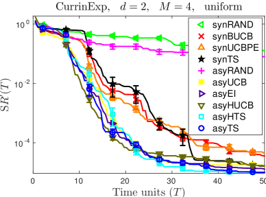
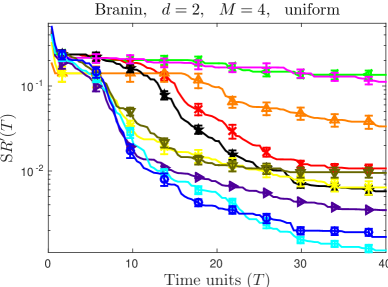
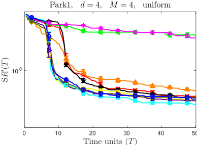
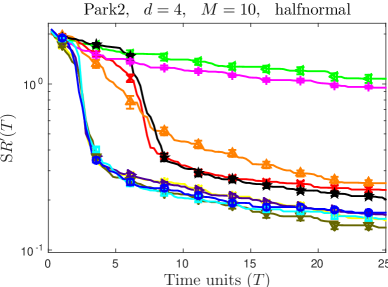
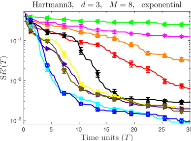
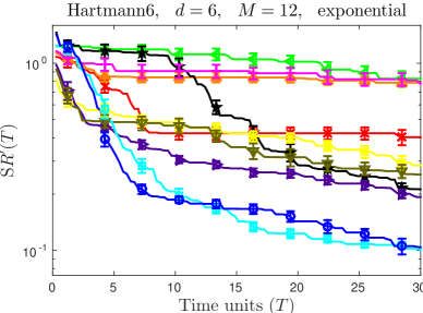
Figure 4: Results on the synthetic experiments. The title states the function used, its dimensionality $d$, the number of workers $M$ and the distribution used for the time. All distributions were constructed so that the expected time for one evaluation was one time unit (for e.g., in the half normal $\mathcal{H}\mathcal{N}(\zeta^{2})$ in Table 1, we used $\zeta=\sqrt{\pi/2}\;$). All figures were averaged over at least $15$ experiments.

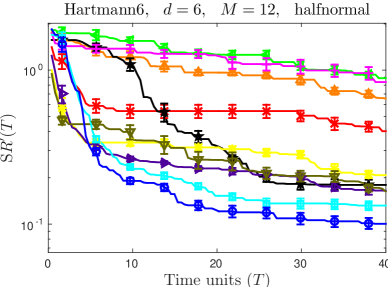
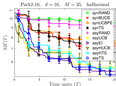
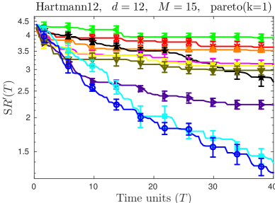
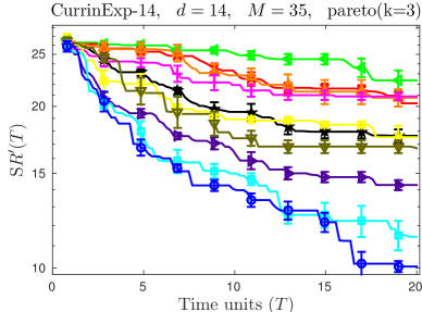
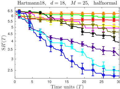
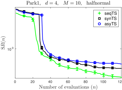
Figure 5: The first five panels are results on synthetic experiments. See caption under Figure 4 for more details. The last panel compares seqTS, synTS, and asyTS against the number of evaluations $n$.

References

- Abadi et al. [2016] Martín Abadi, Ashish Agarwal, Paul Barham, Eugene Brevdo, Zhifeng Chen, Craig Citro, Greg S Corrado, Andy Davis, Jeffrey Dean, Matthieu Devin, Sanjay Ghemawat, Ian Goodfellow, Andrew Harp, Geoffrey Irving, Michael Isard, Yangqing Jia, Rafal Jozefowicz, Lukasz Kaiser, Manjunath Kudlur, Josh Levenberg, Dan Mane, Rajat Monga, Sherry Moore, Derek Murray, Chris Olah, Mike Schuster, Jonathon Shlens, Benoit Steiner, Ilya Sutskever, Kunal Talwar, Paul Tucker, Vincent Vanhoucke, Vijay Vasudevan, Fernanda Viegas, Oriol Vinyals, Pete Warden, Martin Wattenberg, Martin Wicke, Yuan Yu, and Xiaoqiang Zheng. Tensorflow: Large-scale machine learning on heterogeneous distributed systems. arXiv:1603.04467, 2016.
- Adler [1990] Robert J Adler. An Introduction to Continuity, Extrema, and Related Topics for General Gaussian Processes. 1990.
- Agrawal and Goyal [2012] Shipra Agrawal and Navin Goyal. Analysis of thompson sampling for the multi-armed bandit problem. In Conference on Learning Theory (COLT), 2012.
- Boucheron and Thomas [2012] Stéphane Boucheron and Maud Thomas. Concentration inequalities for order statistics. Electronic Communications in Probability, 2012.
- Boucheron et al. [2013] Stéphane Boucheron, Gábor Lugosi, and Pascal Massart. Concentration inequalities: A nonasymptotic theory of independence. Oxford University Press, 2013.
- Chowdhury and Gopalan [2017] Sayak Ray Chowdhury and Aditya Gopalan. On kernelized multi-armed bandits. arXiv:1704.00445, 2017.
- Contal et al. [2013] Emile Contal, David Buffoni, Alexandre Robicquet, and Nicolas Vayatis. Parallel Gaussian process optimization with upper confidence bound and pure exploration. In European Conference on Machine Learning (ECML/PKDD), 2013.
- Desautels et al. [2014] Thomas Desautels, Andreas Krause, and Joel W Burdick. Parallelizing exploration-exploitation tradeoffs in Gaussian process bandit optimization. Journal of Machine Learning Research (JMLR), 2014.
- Ghosal and Roy [2006] Subhashis Ghosal and Anindya Roy. Posterior consistency of Gaussian process prior for nonparametric binary regression". Annals of Statistics, 2006.
- Ginsbourger et al. [2011] David Ginsbourger, Janis Janusevskis, and Rodolphe Le Riche. Dealing with asynchronicity in parallel gaussian process based global optimization. In Conference of the ERCIM WG on Computing and Statistics, 2011.
- Gonzalez et al. [2014] Javier Gonzalez, Joseph Longworth, David James, and Neil Lawrence. Bayesian Optimization for Synthetic Gene Design. In NIPS Workshop on Bayesian Optimization in Academia and Industry, 2014.
- González et al. [2015] Javier González, Zhenwen Dai, Philipp Hennig, and Neil D Lawrence. Batch Bayesian Optimization via Local Penalization. arXiv:1505.08052, 2015.
- He et al. [2016] Kaiming He, Xiangyu Zhang, Shaoqing Ren, and Jian Sun. Deep residual learning for image recognition. In IEEE Conference on Computer Vision and Pattern Recognition (CVPR), 2016.
- Hernández-Lobato et al. [2016] José Miguel Hernández-Lobato, Edward Pyzer-Knapp, Alan Aspuru-Guzik, and Ryan P Adams. Distributed Thompson Sampling for Large-scale Accelerated Exploration of Chemical Space. In NIPS Workshop on Bayesian Optimization, 2016.
- Hutter et al. [2011] Frank Hutter, Holger H Hoos, and Kevin Leyton-Brown. Sequential model-based optimization for general algorithm configuration. In LION, 2011.
- Israelsen et al. [2017] Brett W Israelsen, Nisar R Ahmed, Kenneth Center, Roderick Green, and Winston Bennett. Towards adaptive training of agent-based sparring partners for fighter pilots. In Information Systems. 2017.
- Janusevskis et al. [2012] Janis Janusevskis, Rodolphe Le Riche, David Ginsbourger, and Ramunas Girdziusas. Expected Improvements for the Asynchronous Parallel Global Optimization of Expensive Functions: Potentials and Challenges. In Learning and Intelligent Optimization, 2012.
- Jones et al. [1993] D. R. Jones, C. D. Perttunen, and B. E. Stuckman. Lipschitzian Optimization Without the Lipschitz Constant. J. Optim. Theory Appl., 1993.
- Jones et al. [1998] Donald R. Jones, Matthias Schonlau, and William J. Welch. Efficient global optimization of expensive black-box functions. J. of Global Optimization, 1998.
- Joulani et al. [2013] Pooria Joulani, Andras Gyorgy, and Csaba Szepesvári. Online learning under delayed feedback. In International Conference on Machine Learning (ICML), 2013.
- Jun et al. [2016] Kwang-Sung Jun, Kevin Jamieson, Robert Nowak, and Xiaojin Zhu. Top arm identification in multi-armed bandits with batch arm pulls. In Artificial Intelligence and Statistics (AISTATS), 2016.
- Kandasamy et al. [2015] Kirthevasan Kandasamy, Jeff Schenider, and Barnabás Póczos. High Dimensional Bayesian Optimisation and Bandits via Additive Models. In International Conference on Machine Learning, 2015.
- Kandasamy et al. [2016] Kirthevasan Kandasamy, Gautam Dasarathy, Junier Oliva, Jeff Schenider, and Barnabás Póczos. Gaussian Process Bandit Optimisation with Multi-fidelity Evaluations. In Advances in Neural Information Processing Systems (NIPS), 2016.
- Kathuria et al. [2016] Tarun Kathuria, Amit Deshpande, and Pushmeet Kohli. Batched gaussian process bandit optimization via determinantal point processes. In Advances in Neural Information Processing Systems (NIPS), 2016.
- Krizhevsky and Hinton [2009] Alex Krizhevsky and Geoffrey Hinton. Learning multiple layers of features from tiny images, 2009.
- Martinez-Cantin et al. [2007] R. Martinez-Cantin, N. de Freitas, A. Doucet, and J. Castellanos. Active Policy Learning for Robot Planning and Exploration under Uncertainty. In Proceedings of Robotics: Science and Systems, 2007.
- Osband et al. [2016] Ian Osband, Charles Blundell, Alexander Pritzel, and Benjamin Van Roy. Deep exploration via bootstrapped dqn. In Advances in Neural Information Processing Systems (NIPS), 2016.
- Parkinson et al. [2006] David Parkinson, Pia Mukherjee, and Andrew R Liddle. A Bayesian model selection analysis of WMAP3. Physical Review, 2006.
- Quanrud and Khashabi [2015] Kent Quanrud and Daniel Khashabi. Online learning with adversarial delays. In Advances in Neural Information Processing Systems (NIPS), 2015.
- Rasmussen and Williams [2006] C.E. Rasmussen and C.K.I. Williams. Gaussian Processes for Machine Learning. Adaptative computation and machine learning series. University Press Group Limited, 2006.
- Russo and Van Roy [2014] Dan Russo and Benjamin Van Roy. Learning to optimize via information-directed sampling. In Advances in Neural Information Processing Systems (NIPS), 2014.
- Russo and Van Roy [2016] Daniel Russo and Benjamin Van Roy. An Information-theoretic analysis of Thompson sampling. Journal of Machine Learning Research (JMLR), 2016.
- Seeger et al. [2008] MW. Seeger, SM. Kakade, and DP. Foster. Information Consistency of Nonparametric Gaussian Process Methods. IEEE Transactions on Information Theory, 2008.
- Shah and Ghahramani [2015] Amar Shah and Zoubin Ghahramani. Parallel predictive entropy search for batch global optimization of expensive objective functions. In Advances in Neural Information Processing Systems (NIPS), 2015.
- Snoek et al. [2012] Jasper Snoek, Hugo Larochelle, and Ryan P Adams. Practical Bayesian Optimization of Machine Learning Algorithms. In Advances in Neural Information Processing Systems, 2012.
- Srinivas et al. [2010] Niranjan Srinivas, Andreas Krause, Sham Kakade, and Matthias Seeger. Gaussian Process Optimization in the Bandit Setting: No Regret and Experimental Design. In ICML, 2010.
- Thompson [1933] W. R. Thompson. On the Likelihood that one Unknown Probability Exceeds Another in View of the Evidence of Two Samples. Biometrika, 1933.
- Wang et al. [2016] Jialei Wang, Scott C Clark, Eric Liu, and Peter I Frazier. Parallel Bayesian Global Optimization of Expensive Functions. arXiv:1602.05149, 2016.
- Wang et al. [2017] Zi Wang, Chengtao Li, Stefanie Jegelka, and Pushmeet Kohli. Batched high-dimensional bayesian optimization via structural kernel learning. arXiv:1703.01973, 2017.
- Wu and Frazier [2016] Jian Wu and Peter Frazier. The parallel knowledge gradient method for batch bayesian optimization. In Advances In Neural Information Processing Systems, 2016.