Photon pair generation in a lossy microring resonator. I. Theory

Abstract

We investigate entangled photon pair generation in a lossy microring resonator using an input-output formalism based on the work of Raymer and McKinstrie (Phys. Rev. A 88, 043819 (2013)) and Alsing, et al. (Phys. Rev. A 95, 053828 (2017)) that incorporates circulation factors that account for the multiple round trips of the fields within the cavity. We consider the nonlinear processes of spontaneous parametric down conversion and spontaneous four wave mixing, and we compute the generated biphoton signal-idler state from a single bus microring resonator, along with the generation, coincidence-to-accidental, and heralding efficiency rates. We compare these generalized results to those obtained by previous works employing the standard Langevin input-output formalism.

I Introduction

Over the last decade, advances in chip-based fabrication have made micron-scale, high quality factor Q integrated optical microring resonators (mrr) coupled to an external bus ideal sources of entangled photon pair generation, requiring only $\mu$Ws of pump power Levy et al. (2010); Azzini et al. (2012); Gentry et al. (2015); Preble et al. (2015); Tison et al. (2017); Vernon et al. (2017). Such high-Q mircoring resonators exhibit nonlinear optical properties allowing for biphoton generation arising from the $\chi^{(2)}$ processes of spontaneous parametric down conversion (SPDC), and the $\chi^{(3)}$ processes of spontaneous four-wave mixing (SFWM). Much theoretical research has been devoted to study the generation of entangled photon pair within cavities and mrr in the weak pump field driving limit Scholz et al. (2009); Shen and Fan (2009a, b); Tsang (2011); Camacho (2012); Azzini et al. (2012); Helt et al. (2012); Vernon and Sipe (2015a); Vernon et al. (2015), and more recently in the strong pump field regime Vernon and Sipe (2015b) where higher order nonlinear effects such as self-phase and cross-phase modulation become important.

The predominant method of analysis for analyzing a driven cavity or mrr is the standard Langevin input-output formalism Collet and Gardiner (1984); Walls and Milburn (1994); Mandel and Wolf (1995); Scully and Zubairy (1997); Orszag (2000) which allows one to express the output field in terms of the intra-cavity and external driving fields. This formalism is valid in the high cavity Q limit, near cavity resonances, but does not adequately address processes throughout the entire free spectral range of the cavity. In this work we investigate entangled photon pair generation in a microring resonator using a recent input-output formalism based on the work of Raymer and McKinstrie Raymer and McKinstrie (2013) and Alsing, et al. Alsing et al. (2017) that incorporates the circulation factors that account for the multiple round trips of the fields within the cavity. We consider biphoton pair generation within the mrr via both SPDC and SFWM, and compute the generated two-photon signal-idler intra-cavity and output state from a single bus (all-through) microring resonator. We also compute the two-photon generation, coincidence-to-accidental, and heralding efficiency rates. We compare our results to related calculations Scholz et al. (2009); Tsang (2011); Vernon and Sipe (2015a) obtained using the standard Langevin input-output formalism.

This paper is organized as follows. In Section II we derive and solve the equations of motion for the pump, signal and idler fields within a mrr coupled to a single external bus using a combination of the formalism of Raymer and McKinstrie Raymer and McKinstrie (2013) and Alsing, et al. Alsing et al. (2017). We consider the weak, non-depleted pump field limit where higher order nonlinear processes such as self-phase and cross-phase modulations effects are neglected. We also examine the commutators of the quantum noise fields introduced to account for internal propagation loss which need not commute within the mrr, a phenomena noted by previous authors Barnett Barnett et al. (1996) and Agarwal Huang and Agarwal (2014) in their study of circulating cavity fields. In contrast to the standard Langevin approach, we show these commutators, which can be uniquely solved for by requiring the unitarity of the input and output fields, contain pump dependent contributions. In Section III we compute the output biphoton state, and calculate its generation rate, along with the coincidence to accidental, and heralding efficiency rates. In Section IV we compute the biphoton state generated within the mrr, since this is the state most often calculated in the literature and affords the most straightforward comparison. Again, we calculate the biphoton generation-, coincidence to accidental, and heralding efficiency rates. We investigate how the mrr self-coupling (bus-bus, mrr-mrr) and internal propagation loss effects these rates. In Section V we summarize our results and indicate avenues for future research. In the Appendix A we examine the our expressions for the output fields, and for rates derived from them, in the high cavity Q limit where the standard Langevin input-output formalism is valid, and compare with prior works in the literature.

II SPDC and SPFM processes inside a (single bus) microring resonator

II.1 Preliminaries

In this section we examine the nonlinear processes of spontaneous parametric down conversion (SPDC) and spontaneous four wave mixing (SFWM) inside a single bus microring resonator (mrr) of length $L=2\pi R$, as illustrated in Fig.(1). Here, $a$ is the intracavity field which is coupled to a waveguide bus with input field $a_{in}$ and output field $a_{out}$.

Figure 1: A single bus (all-through) microring resonator (mrr) of length $L=2\pi R$ with intracavity field $a$, coupled to a waveguide bus with input field $a_{in}$ and output field $a_{out}$. $\rho_{a}\,\tau_{a}$ are the beam splitter like self-coupling and cross-coupling strengths, respectively, of the bus to the mrr such that $|\rho_{a}|^{2}+|\tau_{a}|^{2}=1$. $z=0_{+}$ is the point just inside the mrr which cross-couples to the input field $a_{in}$, and $z=L_{-}$ is the point after one round trip in the mrr that cross-couples to the output field $a_{out}$.

The parameters $\rho_{a},\,\tau_{a}$ are the beam splitter like self-coupling and cross-coupling strengths, respectively, of the bus to the mrr such that $|\rho_{a}|^{2}+|\tau_{a}|^{2}=1$. $z=0_{+}$ is the point just inside the mrr which cross-couples to the input field $a_{in}$, and $z=L_{-}$ is the point after on round trip in the mrr that cross-couples to the output field $a_{out}$.

In the work of Raymer and McKinstrie Raymer and McKinstrie (2013) (abbreviated as RM) the cavity field $a$ satisfies a traveling-wave Maxwell ODE in the absence of internal propagation loss given by

$$(\partial_{t}+v_{a}\,\partial_{z})\,a(z,t)=\alpha_{polz}\,P(z,t),$$ (1)

where $a(z,t)$ is the ring resonator cavity field (in the time domain), $v_{a}$ is the group velocity, $P(z,t)$ is the polarization and $\alpha_{polz}$ is a coupling constant. The carrier wave frequency has been factored out so that all frequencies are relative to the optical carrier frequency. The input coupling and periodicity of the cavity is captured by the boundary conditions

$$a(0_{+},t) = \rho_{a}\,a(L_{-},t)+\tau_{a}\,a_{in}(t),$$ (2a)

$$a_{out}(t) = \tau_{a}\,a(L_{-},t)-\rho_{a}\,a_{in}(t),$$ (2b)

where we have taken the beam splitter like self-coupling $\rho_{a}$ (buss-bus, mrr-mrr), and cross-coupling $\tau_{a}$ (bus-mrr) real for simplicity and the minus sign in Eq.(2b) accounts for the $\pi$ change in phase arising from the ”reflection” of the input field off the higher index of refraction mrr to the output (bus) field. The input and output fields satisfy the free field commutators

$$[a_{in}(t),a_{in}^{\dagger}(t^{\prime})]=\delta(t-t^{\prime})=[a_{out}(t),a_{out}^{\dagger}(t^{\prime})].$$ (3)

The output field $a_{out}({\omega})$ is easily solved from Eq.(1), Eq.(2a) and Eq.(2b) in the Fourier domain yielding the unimodular transfer function $G_{out,in}({\omega})$ defined by

$$a_{out}({\omega})\equiv G_{out,in}({\omega})\,a_{in}({\omega}),\qquad G_{out,in}({\omega})=e^{i{\omega}T_{a}}\,\left[\frac{1-\rho_{a}\,e^{-i{\omega}T_{a}}}{1-\rho_{a}\,e^{i{\omega}T_{a}}}\right],\qquad|G_{out,in}({\omega})|=1.$$ (4)

Note that in the classical case (see e.g. YarivYariv (2000), and Rabus Rabus (2007)) one obtains the result with phenomenological loss factor $0\leq\alpha_{a}\leq 1$

$$a_{out}({\omega})\equiv G^{(\alpha)}_{out,in}({\omega})\,a_{in}({\omega})=\left(\frac{\alpha_{a}\,e^{i\theta_{a}}-\rho_{a}}{1-\rho_{a}^{*}\,\alpha_{a}\,e^{i\theta_{a}}}\right)\,a_{in}({\omega}),\qquad|G^{(\alpha)}_{out,in}({\omega})|\leq 1,$$ (5)

which is the same coefficient that appears in the quantum derivation with loss (see Eq.(13g) in Alsing et al. Alsing et al. (2017) (abbreviated as AH) with $\rho_{a}\rightarrow\tau_{a}$ real) and $\theta_{a}={\omega}\,T_{a}$. The lossless case corresponds to $\alpha_{a}\rightarrow 1$.

For the quantum derivation including internal propagation loss (generalizing the the lossless mrr considerations begun in Hach III et al. (2014)), AH Alsing et al. (2017) used an expression by Loudon Barnett et al. (1997); Loudon (2000) for the attenuation loss of a traveling wave, modeled from a continuous set of beams splitters acting as scattering centers Barnett et al. (1997); Loudon (2000),

$$a(L_{-},{\omega})=e^{i\xi_{a}(\omega)L}\,a(0_{+},\omega)+i\sqrt{{\Gamma}_{a}(\omega)}\,\int_{0}^{L}dz\,e^{i\xi_{a}(\omega)(L-z)}\,s(z,\omega),$$ (6)

where $e^{i\xi_{a}L}\equiv\alpha_{a}\,e^{i\,\theta_{a}}$ with $\alpha_{a}=e^{-\frac{1}{2}\,({\Gamma}_{a}/v_{a})\,L}$, $\theta_{a}=({\omega}\,n({\omega})/c)\,L=\omega\,T_{a}$ and ${\Gamma}_{a}$ incorporates both coupling and internal propagation losses. Here, $s(z,\omega)$ are the noise scattering operators that give rise to the internal loss and satisfy $[s(z,\omega),s^{\dagger}(z^{\prime},\omega^{\prime})]=\delta(z-z^{\prime})\,\delta({\omega}-{\omega}^{\prime})$. AH explicitly showed that $a(L_{-},{\omega})$ in Eq.(6) satisfied $[a(L_{-},{\omega}),a^{\dagger}(L_{-},{\omega}^{\prime})]=\delta({\omega}-{\omega}^{\prime})$. By tracking the infinite number of round trip circulations of the cavity field in the single bus mrr, AH derive the expression (with $\tau\rightarrow\rho_{a}$ and $\kappa\rightarrow\tau_{a}$ in Alsing et al. (2017))

$$a_{out}({\omega})=\left(\frac{\rho_{a}-\alpha_{a}\,e^{i\theta_{a}}}{1-\rho^{*}_{a}\,\alpha_{a}\,e^{i\theta_{a}}}\right)\,a_{in}({\omega})-i|\tau_{a}|^{2}\,\sqrt{{\Gamma}_{a}}\sum_{n=0}^{\infty}(\rho_{a})^{n}\,\int_{0}^{(n+1)L}dz\,e^{i\xi_{a}(\omega)[(n+1)L-z]}\hat{s}(z,\omega).$$ (7)

AH show by explicit calculation that the output field satisfies $[a_{out}({\omega}),a_{out}^{\dagger}({\omega})]=\delta({\omega}-{\omega}^{\prime})$. In general, this allows one to write

$$a_{out}({\omega})=G_{out,in}({\omega})\,a_{in}+H_{out,in}({\omega})\,f_{a}({\omega}),\quad|H_{out,in}({\omega})|=\sqrt{1-|G_{out,in}({\omega})|^{2}},$$ (8)

which defines the quantum noise operator $f_{a}({\omega})$ from the unitary requirement of the preservation of the free field output commutator. In the Appendix A we examine $G_{out,in}({\omega})$ and $H_{out,in}({\omega})$ in the high cavity Q limit, where the standard Langevin input-output formalism is valid.

II.2 Derivation of output operators from input and noise operators

For the consideration of nonlinear biphoton pair generation, we now consider three intracavity fields circulating within the mrr: the signal field $a(z,t)$, the idler field $b(z,t)$ and the pump field $c(z,t)$. As in the previous section, we work in the interaction picture where the carrier frequencies ${\omega}_{d}$ for $d\in\{a,b,c\}$ have been removed, so that the fields are slowly varying in time. In the interaction picture the nonlinear Hamiltonian for these processes are taken to be

$$\mathcal{H}^{NL}_{spdc} = g_{spdc}\,\left(c\,a^{\dagger}\,b^{\dagger}+h.a.\right),\quad\quad\qquad{\omega}_{c}={\omega}_{a}+{\omega}_{b},$$ (9a)

$$\mathcal{H}^{NL}_{sfwm} = g_{sfwm}\,\left(c^{2}\,a^{\dagger}\,b^{\dagger}+h.a.\right),\qquad 2\,{\omega}_{c}={\omega}_{a}+{\omega}_{b}.$$ (9b)

Each field $d(z,t)$ for $d\in\{a,b,c\}$ satisfies the equation of motion and input-output boundary conditions

$$(\partial_{t}+v_{d}\,\partial_{z})\,d(z,t) = -i\,[d(z,t),\mathcal{H}^{NL}]-\frac{{\gamma}^{\prime}_{d}}{2}\,d(z,t)+\alpha_{polz}\,F_{d}(z,t),$$ (10a)

$$d(0_{+},t) = \rho_{d}\,d(L_{-},t)+\tau_{d}\,d_{in}(t),$$ (10b)

$$d_{out}(t) = \tau_{d}\,d(L_{-},t)-\rho_{d}\,d_{in}(t),$$ (10c)

where we have included the internal mrr propagation loss given by the rate $\gamma^{\prime}_{d}$. We also allow for different group velocities $v_{d}({\omega})=c/n_{d}({\omega})$ for each mode $d$ leading to different round trip times $T_{d}=L/v_{d}$ for $k\in\{a,b,c\}$. Junction coupling losses between the ring resonator and the bus are taken into account by later defining the self-coupling loss $\gamma_{d}$ via $\rho_{d}\equiv e^{-\gamma_{d}\,T_{d}/2}$ Raymer and McKinstrie (2013).

In the above $F_{d}(z,t)$ are the noise operators inside the ring resonator and $\alpha_{polz}$ is a coupling constant of the internal modes $a,b$ to the polarization field, giving rise to internal loss (see RM Raymer and McKinstrie (2013)). While the noise operators could be derived directly as in AH Alsing et al. (2017) by tracking the multiple round trips of each field $d$ through the mrr, here we have opted for the Langevin-based approach indicated (but not explored) in RM Raymer and McKinstrie (2013). Here, we differ from RM by not explicitly indicating the value of the commutation relations for the noise operators $F_{d}(z,t)$, preferring instead to compute their values later by the causality condition that the output fields $d_{out}$ of the above coupled set of equations satisfy the free field canonical commutation relations, given that the input fields $d_{in}$ do. The particular value of the commutators are important when we compute the reduced density matrix $\rho_{ab}$ for the two-photon output signal-idler state. For now the noise operators $F_{d}$ are simply carried along through the computation.

The above equations are most easily solved in the frequency domain (using $d(z,{\omega})=\int_{-\infty}^{\infty}dt\,d(z,t)\,e^{i{\omega}\,t}$, for $d\in\{a,b,c\}$, and $f_{d}(z,{\omega})=\int_{-\infty}^{\infty}dt\,F_{d}(z,t)\,e^{i{\omega}\,t}$). Here the interaction Hamiltonians are given by

$$\mathcal{H}^{NL}_{spdc} = \int_{-\infty}^{\infty}\,\frac{d{\omega}}{2\pi}\,g_{spdc}({\omega})\,\left(c(z,{\omega})\,a^{\dagger}(z,{\omega})\,b^{\dagger}(z,{\omega})+h.a.\right),\quad g_{spdc}({\omega})=\frac{3\,(\hbar\,{\omega}_{c})^{3/2}\,\chi^{(2)}}{4\epsilon_{0}\,\bar{n}^{4}\,V_{ring}},\qquad$$ (11a)

$$\mathcal{H}^{NL}_{sfwm} = \int_{-\infty}^{\infty}\,\frac{d{\omega}}{2\pi}\,g_{sfwm}({\omega})\,\left(c^{2}(z,{\omega})\,a^{\dagger}(z,{\omega})\,b^{\dagger}(z,{\omega})+h.a.\right),\quad g_{sfwm}({\omega})=\frac{3(\hbar\,{\omega}_{c})^{2}\,\chi^{(3)}}{4\epsilon_{0}\,\bar{n}^{4}\,V_{ring}},\qquad.$$ (11b)

where the value of $g_{spdc}({\omega})$ and $g_{sfwm}({\omega})$ Helt et al. (2012); Vernon and Sipe (2015a) depend on the volume $V_{ring}$ of the ring mode, and the nonlinear susceptibilities $\chi^{(2)}$ and $\chi^{(3)}$ are accessed uniformly in the ring. Here $\bar{n}$ is the average index of refraction of the ring (assumed constant) and $\epsilon_{0}$ is the permittivity of free space.

In the undepleted pump approximation, employed here, the equation of motion for the pump mode $c$ satisfies Eq.(1) (with $a\rightarrow c$ and $P(z,t)=0$), and Hamiltonian terms such as $-i\,g_{spdc}\,a\,b$ and $-i\,g_{sfwm}\,c^{\dagger}\,a\,b$ are considered small, and hence dropped along with the noise term $f_{c}$ . This equation is then classical, and the value of the lossless pump inside the ring becomes

$$\langle c(0_{+},{\omega})\rangle=\frac{\tau_{c}}{1-\rho_{c}\,e^{i{\omega}T_{c}}}\,\langle c_{in}({\omega})\rangle,\quad\langle c(L_{-},{\omega})\rangle=\frac{\tau_{c}\,e^{i{\omega}T_{c}}}{1-\rho_{c}\,e^{i{\omega}T_{c}}}\,\langle c_{in}({\omega})\rangle.$$ (12)

where the angled brackets indicate that we are dealing with a c-number field value. Outside the ring, the pump field is given by

$$\langle c_{out}({\omega})\rangle\equiv G_{c_{out}\,c_{in}}({\omega})\,\langle c_{in}({\omega})\rangle,\qquad G_{c_{out}\,c_{in}}({\omega})=e^{i{\omega}T_{c}}\,\left[\frac{1-\rho_{c}\,e^{-i{\omega}T_{c}}}{1-\rho_{c}\,e^{i{\omega}T_{c}}}\right].$$ (13)

Therefore, in the Hamiltonian we replace the operator $c_{p}$ by $\langle c(z,{\omega})\rangle$ and write

$$\mathcal{H}^{NL} = \int_{-\infty}^{\infty}\,\frac{d{\omega}}{2\pi}\,g({\omega})\,\left(\alpha_{p}(z,{\omega})\,a^{\dagger}(z,{\omega})\,b^{\dagger}(z,{\omega})+\alpha^{*}_{p}(z,{\omega})\,a(z,{\omega})\,b(z,{\omega})\right),$$ (14a)

$$g({\omega}) = g_{spcd}({\omega}),\quad\;\;\alpha_{p}(z,{\omega})=\langle c(z,{\omega})\rangle\;\;\textrm{for SPDC},$$ (14b)

$$g({\omega}) = g_{sfwm}({\omega}),\quad\alpha_{p}(z,{\omega})=\langle c^{2}(z,{\omega})\rangle\;\;\textrm{for SFWM}.$$ (14c)

Thus, for both nonlinear processes the signal and idler modes satisfy the equation of motion in the frequency domain

$$(-i\,{\omega}+v_{a}\,\partial_{z})\,a(z,{\omega}) = -i\,g\,\alpha_{p}(z,{\omega})\,b^{\dagger}(z,{\omega})-\frac{{\gamma}^{\prime}_{a}}{2}\,a(z,{\omega})+\alpha_{polz}\,f_{a}(z,{\omega}),$$ (15a)

$$(-i\,{\omega}+v_{b}\,\partial_{z})\,b^{\dagger}(z,{\omega}) = i\,g\,\alpha^{*}_{p}(z,{\omega})\,a(z,{\omega})-\frac{{\gamma}^{\prime}_{b}}{2}\,b^{\dagger}(z,{\omega})+\alpha_{polz}\,f_{b}(z,{\omega}).$$ (15b)

Eq.(15a) has the formal solution

$$a(L_{-},{\omega})=a(0_{+},t)\,e^{i\xi_{a}L}+\int_{0}^{L}dz^{\prime}\,\left((-ig\alpha_{P}/v_{a})\,b^{\dagger}(z^{\prime},{\omega})+(\alpha_{polz}/v_{a})\,\tilde{f}_{a}(z^{\prime},{\omega})\right)\,e^{i\,\xi_{a}(L-z^{\prime})}$$ (16)

where $\xi_{a}=({\omega}+i\,\gamma^{\prime}_{a}/2)/v_{a}$ so that $i\,\xi_{a}L=(i{\omega}-\,\gamma^{\prime}_{a}/2)\,T_{a}$. For fast molecular damping we approximate the last term by setting $z^{\prime}\rightarrow L$ (the upper limit of the integral) and factoring out $\alpha_{p}(L_{-},{\omega})\,b^{\dagger}(L_{-},{\omega})$ from the integral. The remaining integral yields $(-i\,g\,\alpha_{p}(L_{-},{\omega})/v_{a})\,\int_{0}^{L}dz^{\prime}\,e^{i\,\xi_{a}(L-z^{\prime})}$ $=(-ig\alpha_{p}(L_{-},{\omega})/v_{a})(1-e^{i\xi_{a}L})/(-i\xi_{a})\rightarrow-ig\,\alpha_{p}(L_{-},{\omega})\,T_{a}\equiv-i\,r_{a}({\omega})$ defining the dimensionless pump parameter $r_{a}({\omega})=g\,\alpha_{p}({\omega})\,T_{a}$. Thus, we write Eq.(16) as

$$a(L_{-},{\omega})=a(0_{+},t)\,e^{i\xi_{a}L}-i\,r_{a}({\omega})\,b^{\dagger}(L_{-},t)+f_{a}({\omega}),\quad f_{a}({\omega})\equiv(\alpha_{polz}/v_{a})\int_{0}^{L}dz^{\prime}\,\tilde{f}_{a}(z^{\prime},{\omega})\,e^{i\,\xi_{a}(L-z^{\prime})}.\qquad\qquad$$ (17a)

Similarly, Eq.(15b) yields

$$b^{\dagger}(L_{-},{\omega})=b^{\dagger}(0_{+},t)\,e^{i\xi_{b}L}+i\,r_{b}({\omega})\,a(L_{-},t)+f^{\dagger}_{b}({\omega}),\;f^{\dagger}_{b}({\omega})=(\alpha_{polz}/v_{a})\int_{0}^{L}dz^{\prime}\,\tilde{f}^{\dagger}_{b}(z^{\prime},{\omega})\,e^{i\,\xi_{b}(L-z^{\prime})},\qquad\qquad$$ (17b)

where we have defined $f_{a}({\omega})$ and $f^{\dagger}_{b}({\omega})$ and used the notation $r_{a}({\omega})\equiv g\,\alpha_{p}(L_{-},{\omega})\,T_{a}$ and $r_{b}({\omega})\equiv g\,\alpha^{*}_{p}(L_{-},{\omega})\,T_{b}$. We can therefore put equations of motion and boundary conditions for the signal $a$ and idler $b$ modes in matrix form as

$$M\,\vec{a}(L_{-},{\omega}) = P_{\xi}\,\vec{a}(0_{+},{\omega})+\vec{f}({\omega}),$$ (18a)

$$\vec{a}(0_{+},{\omega}) = T_{\rho}\,\vec{a}(L_{-},{\omega})+X_{\tau}\,\vec{a}_{in}({\omega}),$$ (18b)

$$\vec{a}_{out}({\omega}) = X_{\tau}\,\vec{a}(L_{-},{\omega})-T_{\rho}\,\vec{a}_{in}({\omega}),$$ (18c)

where we have defined

$$M=\left(\begin{array}[]{cc}1&i\,r_{a}\\ -i\,r_{b}&1\\ \end{array}\right),\;P_{\xi}=\left(\begin{array}[]{cc}e^{i\xi_{a}L}&0\\ 0&e^{i\xi_{b}L}\\ \end{array}\right),\;T_{\rho}=\left(\begin{array}[]{cc}\rho_{a}&0\\ 0&\rho_{b}\\ \end{array}\right),\;X_{\tau}=\left(\begin{array}[]{cc}\tau_{a}&0\\ 0&\tau_{b}\\ \end{array}\right),$$ (19)

and

$$\vec{a}({\omega})=\left(\begin{array}[]{c}a({\omega})\\ b^{\dagger}({\omega})\\ \end{array}\right),\quad\vec{a}_{in}({\omega})=\left(\begin{array}[]{c}a_{in}({\omega})\\ b_{in}^{\dagger}({\omega})\\ \end{array}\right),\quad\vec{a}_{out}({\omega})=\left(\begin{array}[]{c}a_{out}({\omega})\\ b_{out}^{\dagger}({\omega})\\ \end{array}\right),\quad\vec{f}({\omega})=\left(\begin{array}[]{c}f_{a}({\omega})\\ f_{b}^{\dagger}({\omega})\\ \end{array}\right).\qquad\qquad$$ (20)

Here $T_{\rho}$ represents the through coupling ‘reflection’ from input bus off the ring resonator to output bus (and the self-coupling within the mrr), while $X_{\tau}$ represents the cross coupling ‘transmission’ between the bus and the ring resonator. The term $P_{\xi}$ represents the roundtrip phase accumulation and intrinsic loss within the ring resonator, and we define $e^{i\xi_{k}L}\equiv\alpha_{k}\,e^{i\theta_{k}}$ with $\alpha_{k}=e^{-\gamma^{\prime}_{k}\,T_{k}/2}$ and $\theta_{k}={\omega}\,T_{k}$, $r_{a}=g\,\alpha_{p}\,T_{a}$, and $r_{b}=g\,\alpha^{*}_{p}\,T_{b}$.

A substitution of $\vec{a}(0_{+},{\omega})$ from Eq.(18b) into the right hand side of Eq.(18a) allows for the solution of the intracavity field (just before exit) $\vec{a}(L_{-},{\omega})$ in terms of $\vec{a}_{in}({\omega})$ and $\vec{f}({\omega})$. A subsequent substitution of this solution for $\vec{a}(L_{-},{\omega})$ into the right hand side of Eq.(18c) produces the desired output field $\vec{a}_{out}({\omega})$ in terms of the input field $\vec{a}_{in}({\omega})$ and noise operators $\vec{f}({\omega})$. After some lengthy but straightforward algebra, the output fields can be expressed in terms of the input fields as

$$\vec{a}_{out}({\omega})=G({\omega})\,\vec{a}_{in}({\omega})+H({\omega})\,\vec{f}({\omega}),$$ (21)

where

$$G({\omega}) = \left[X_{\tau}(M-P_{\xi}\,T_{\rho})^{-1}\right]P_{\xi}\,X_{\tau}-T_{\rho}\equiv\left(\begin{array}[]{cc}G_{aa}({\omega})&G_{ab}({\omega})\\ G_{ba}({\omega})&G_{bb}({\omega})\\ \end{array}\right),$$ (22c)

$$\equiv \frac{1}{D}\left(\begin{array}[]{cc}(e^{i\xi_{a}L}-\rho_{a})\,(1-\rho_{b}\,e^{i\xi_{b}L})+r_{a}\,r_{b}\,\rho_{a}&-i\,r_{a}\,\tau_{a}\,\tau_{b}\,e^{i\xi_{b}L}\\ i\,r_{b}\,\tau_{b}\,\tau_{a}\,e^{i\xi_{a}L}&(e^{i\xi_{b}L}-\rho_{b})\,(1-\rho_{a}\,e^{i\xi_{a}L})+r_{a}\,r_{b}\,\rho_{b}\\ \end{array}\right),\qquad$$ (22f)

with

$$D = (1-\rho_{a}\,e^{i\xi_{a}L})\,(1-\rho_{b}\,e^{i\xi_{b}L})-r_{a}\,r_{b},\qquad r_{a}=g\alpha_{P}T_{a}\,\quad\,r_{b}=g\alpha^{*}_{P}T_{b},$$ (23a)

$$\alpha_{k} = e^{-\gamma^{\prime}_{k}/2\,T_{k}},\quad\theta_{k}={\omega}\,T_{k},\quad\textrm{for}\quad k\in\{a,b\},$$ (23b)

and

$$H({\omega})=X_{\tau}(M-P_{\xi}\,T_{\rho})^{-1}\equiv\left(\begin{array}[]{cc}H_{aa}({\omega})&H_{ab}({\omega})\\ H_{ba}({\omega})&H_{bb}({\omega})\\ \end{array}\right)=\frac{1}{D}\,\left(\begin{array}[]{cc}\tau_{a}\,(1-\rho_{b}e^{i\xi_{b}L})&-i\,r_{a}\,\tau_{a}\\ i\,r_{b}\,\tau_{b}&\tau_{b}\,(1-\rho_{a}e^{i\xi_{a}L})\end{array}\right).\qquad$$ (24)

Note that to lowest order in $|g\alpha_{p}|$, we have $1/D\approx S_{a}\,S_{b}$ where $S_{k}=\frac{1}{1-\rho_{k}\,e^{i\xi_{k}L}}=\sum_{n=0}^{\infty}\,\left(\rho_{k}\,e^{i\xi_{k}L}\right)^{n}\equiv\sum_{n=0}^{\infty}\,\left(\rho_{k}\,\alpha_{k}\,e^{i\,\theta_{k}}\right)^{n}$ for $k\in\{a,b\}$ are the geometric series factors resulting from the round trip circulations of the internal fields $k\in\{a,b\}$ inside the ring resonator. For typical ring resonator of radius $R=20\mu$m and pump laser power of 1mW ($\chi^{(2)}\sim 2\times 10^{-12}$ m/V, $\alpha_{p}\sim 10^{3}$ V/m,) and round trip times of $T_{k}\sim$ 1 ps, we have $r_{p}\sim 10^{-5}$ Schneeloch et al. (2017). A comparison of the matrix forms of $G({\omega})$ in Eq.(22c) and $H({\omega})$ in Eq.(24) reveals the useful relationship

$$G({\omega})=H({\omega})\,P_{\xi}({\omega})\,X_{\tau}({\omega})-T_{\rho}({\omega}).$$ (25)

In the Appendix A we examine $G({\omega})$ and $H({\omega})$ in the high cavity Q limit defined by $\rho_{k}\equiv e^{-\gamma_{k}\,T_{k}/2}\rightarrow 1,\;{\omega}\,T_{k}\ll 1$ where the standard Langevin approximation Walls and Milburn (1994); Orszag (2000) is valid, and compare our results with recent related work Tsang (2011) using the later formulation.

II.3 Commutators of the noise operators

II.3.1 Linear equations determined by causality

The commutation relations between the noise operators are fundamentally determined by the canonical commutators of the free input and output fields. Given that the input fields satisfy $[a_{in}({\omega}),a^{\dagger}_{in}({\omega}^{\prime})]=[b_{in}({\omega}),b^{\dagger}_{in}({\omega}^{\prime})]=\delta({\omega}-{\omega}^{\prime})$, and that they each commute with the noise operators $f_{a}({\omega}),\,f_{b}({\omega})$ (via causality), one must also have that $[a_{out}({\omega}),a^{\dagger}_{out}({\omega}^{\prime})]=[b_{out}({\omega}),b^{\dagger}_{out}({\omega}^{\prime})]=\delta({\omega}-{\omega}^{\prime})$. Using Eq.(25), this unitary requirement determines the set of linear equations

$${}[a_{out}({\omega}),a^{\dagger}_{out}({\omega}^{\prime})] = \delta({\omega}-{\omega}^{\prime})\Rightarrow|H_{aa}|^{2}\,C_{aa}-|H_{ab}|^{2}\,C_{bb}+2\textrm{Re}(H_{aa}\,H^{*}_{ab}\,D_{ab})=1-(|G_{aa}|^{2}-|G_{ab}|^{2}),\qquad$$ (26a)

$${}[b_{out}({\omega}),b^{\dagger}_{out}({\omega}^{\prime})] = \delta({\omega}-{\omega}^{\prime})\Rightarrow-|H_{ba}|^{2}\,C_{aa}+|H_{bb}|^{2}\,C_{bb}+2\textrm{Re}(H_{ba}\,H^{*}_{bb}\,D_{ab})=1-(|G_{bb}|^{2}-|G_{ba}|^{2}),\qquad\quad$$ (26b)

$${}[a_{out}({\omega}),b_{out}({\omega}^{\prime})] = 0\Rightarrow H_{aa}\,H^{*}_{ba}\,C_{aa}-H_{ab}\,H^{*}_{bb}\,C_{bb}+H_{aa}\,H^{*}_{bb}\,D_{ab}+H_{ab}\,H^{*}_{ba}\,D^{*}_{ab}=G_{ab}\,G^{*}_{bb}-G_{aa}\,G^{*}_{ba},\qquad$$ (26c)

$${}[a_{out}({\omega}),b^{\dagger}_{out}({\omega}^{\prime})] = 0\Rightarrow\textrm{det}(H)\,C_{ab}=0,$$ (26d)

for the four constants $C_{aa}$, $C_{bb}$, $C_{ab}$, $D_{ab}$ defined by the commutation relations

$${}[f_{a}({\omega}),f^{\dagger}_{a}({\omega}^{\prime})]=C_{aa}\,\delta({\omega}-{\omega}^{\prime}),\quad[f_{b}({\omega}),f^{\dagger}_{b}({\omega}^{\prime})]=C_{bb}\,\delta({\omega}-{\omega}^{\prime}),$$ (27a)

$${}[f_{a}({\omega}),f^{\dagger}_{b}({\omega}^{\prime})]=C_{ab}\,\delta({\omega}-{\omega}^{\prime}),\quad[f_{a}({\omega}),f_{b}({\omega}^{\prime})]=D_{ab}\,\delta({\omega}-{\omega}^{\prime}).$$ (27b)

Since $\textrm{det}(H)\neq 0$, Eq.(26d) reveals that $C_{ab}=0$. The first three equations are four equations in the four (real) unknowns $C_{aa}$, $C_{bb}$, $\textrm{Re}(D_{ab})$, $\textrm{Im}(D_{ab})$ which therefore have a unique solution. Note that in the standard Langevin approach Walls and Milburn (1994); Orszag (2000) one assumes the canonical values $C_{aa}=C_{bb}=1$ and $C_{ab}=D_{ab}=0$. But the standard input-output formalism (here, valid near resonances of the ring resonator) was explicitly constructed so these canonical values identically satisfy the above set of linear equations (see for example the $G$ and $H$ matrices used in Tsang Tsang (2011) and Shapiro Barzanjeh et al. (2015)). These special commutator values are not necessarily valid in general, and in particular $D_{ab}\neq 0$ as pointed out in the works of Barnett Barnett et al. (1996) and Agarwal Huang and Agarwal (2014). In general, the values of $C_{aa}$, $C_{bb}$, $D_{ab}$ must be computed from Eq.(26a), Eq.(26b) and Eq.(26c). The values of these commutators are not only important for the self consistency of the theory, but are also relevant when one computes the accidental singles rate upon the loss of either the generated signal or idler photon due to noise in the ring resonator. However, the values of these commutators do not affect the two-photon portion of the total state (see next section) where neither a signal nor an idler photon is absorbed within the mrr.

II.3.2 Exact solution of the commutator equations

Using the expressions in Eq.(22c) for $G({\omega})$ and Eq.(24) for $H({\omega})$ a long but straightforward calculation results in the following simple exact solutions for the commutator equations Eq.(26a)-Eq.(26c)

$$C_{kk}({\omega}) = 1-\alpha_{k}^{2}-|r_{k}|^{2}=1-e^{-\gamma^{\prime}_{k}T_{k}}-|g\alpha_{p}\,T_{k}|^{2}\hbox{ \raise-5.69054pt\hbox{$\textstyle{\longrightarrow}\atop\scriptstyle{\textrm{high Q}}$} }\gamma^{\prime}_{k}\,T_{k}-|g\alpha_{p}\,T_{k}|^{2},\quad k\in\{a,b\},\qquad$$ (28a)

$$D_{ab} = i\,(r^{*}_{b}-r_{a})=i\,g\,\alpha_{p}\,(T_{b}-T_{a}),$$ (28b)

where for $C_{aa}({\omega})$ and $C_{bb}({\omega})$ we have also indicated their values in the high cavity Q limit. We note that $C_{kk}({\omega})$ for $k\in\{a,b\},$ contains a power dependent correction $|r_{k}|^{2}=|g\,\alpha_{p}\,T_{k}|^{2}$ of higher order than the leading order term $1-\alpha_{k}^{2}$ which approaches $\gamma^{\prime}_{k}\,T_{k}$ is the high Q limit. If we were to redefine the noise operators as $f_{k}({\omega})\equiv(T_{k})^{1/2}\,f^{\prime}_{k}({\omega})$ then $C_{kk}({\omega})\equiv T_{k}\,\tilde{C}_{kk}$ where $\tilde{C}_{kk}=[f^{\prime}_{k}({\omega}),f^{\prime\dagger}_{k}({\omega})]\approx\gamma^{\prime}_{k}\,\delta({\omega}-{\omega}^{\prime})$ to lowest order in $|r_{k}|^{2}$. This is the scaling employed by Raymer and McKinstrie Raymer and McKinstrie (2013) for the intracavity fields when comparing the operator equations of motions in the high Q limit to the standard Langevin approach.

Other authors (see e.g., Tsang (2011); Barzanjeh et al. (2015)) using the standard Langevin approach often simply state from the outset that $[f^{\prime\prime}_{k}({\omega}),f^{\prime\prime\dagger}_{k}({\omega}^{\prime})]=\delta({\omega}-{\omega}^{\prime})$, with the assumption that all cross commutators are zero (i.e. $C_{ab}=D_{ab}=0$), invoking independent noise sources. One could, of course, obtain this form of the diagonal commutators by redefining $f_{k}({\omega})=(C_{kk})^{1/2}\,f^{\prime\prime}_{k}({\omega})$, (with an appropriate rescaling of $H({\omega})$). However, even in the high Q limit we see from Eq.(28b) that the cross commutator $[f_{a}({\omega}),f_{b}({\omega})]=D_{ab}\,\delta({\omega}-{\omega}^{\prime})$ remains non-zero (though small), unless we assume equal group velocities (index of refractions) for both the signal ($a$) and idler ($b$) modes so that $T_{a}=T_{b}$.

III The output two-photon signal-idler state

Inside the ring resonator the Hamiltonian in frequency space is

$$\mathcal{H}^{NL}=\int_{0_{+}}^{L_{-}}dz\int_{-\infty}^{\infty}\frac{d{\omega}}{2\pi}\,g({\omega})\,\left(\alpha_{p}(z,{\omega})\,a^{\dagger}(z,{\omega})\,b^{\dagger}(z,{\omega})+\alpha^{*}_{p}(z,{\omega})\,a(z,{\omega})\,b(z,{\omega})\right).$$ (29)

For a weak driving field $\alpha_{p}({\omega})=|\alpha_{p}({\omega})|\,e^{i\theta_{p}(\omega)}$, the two-photon state inside the mrr is given by

$$|\Psi(T_{ab})\rangle_{ab} = e^{-i\,\mathcal{H}^{NL}\,T_{ab}}\,|\Psi\rangle_{in}\approx\left(1-i\,\mathcal{H}^{NL}\,T_{ab}\right)|\textrm{vac}\rangle$$ (30a)

$$= \left[1-i\int_{-\infty}^{\infty}\frac{d{\omega}}{2\pi}\,r_{ab}({\omega})\,\left(e^{i\theta_{p}(\omega)}\,a^{\dagger}(L_{-},{\omega})\,b^{\dagger}(L_{-},{\omega})+e^{-i\theta_{p}(\omega)}\,a(L_{-},{\omega})\,b(L_{-},{\omega})\right)\right]|\textrm{vac}\rangle,\qquad\quad$$ (30b)

where we have taken $T_{ab}=\sqrt{T_{a}T_{b}}=L/\sqrt{v_{a}\,v_{b}}$ assuming the group velocities of the generated signal and idler photons $v_{a},v_{b}$ are not too different, and $|r_{ab}({\omega})|\equiv|g({\omega})\,\alpha_{p}(L_{-},{\omega})\,T_{ab}|$. For simplicity, in Eq.(30b) we have assumed perfect phase matching and zero dispersion. In general Scholz et al. (2009); Schneeloch and Howell (2016); Schneeloch et al. (2017); Vernon and Sipe (2015a, b), when the field operators inside the mrr are decomposed in terms of their spatial Fourier components the spatial integral produces a phase matching contribution term, $\int_{0_{+}}^{L_{-}}dz\exp{[i\big{(}k_{p}({\omega}_{p})-k_{a}({\omega}_{a})-k_{b}({\omega}_{b})\big{)}\,z}]$ for SPDC and $\int_{0_{+}}^{L_{-}}dz\exp{[i\big{(}2\,k_{p}({\omega}_{p})-k_{a}({\omega}_{a})-k_{b}({\omega}_{b})\big{)}\,z}]$ for SFWM, yielding oscillatory $\sin$c function contributions over the longitudinal momentum conservation mismatch within the mrr. Further, dispersion effects within the mrr could be accounted for by Taylor expanding $k({\omega}_{k})={\omega}_{k}\,n_{k}({\omega}_{k})/c$ about central frequencies ${\omega}_{k,0}$ for $k\in\{p,a,b\}$ to either first or second order. While these spatially modulating $\sin$c factors (which are unity for perfect phase matching) and dispersion effects are important to account for in actual physical devices, we will ignore them here in this work for ease of exposition.

The output state $|\Psi\rangle_{out}$ is obtained from the internal $|\Psi(T_{ab})\rangle_{ab}$ as the Heisenberg operators evolve from inside the mrr to the output bus. Making this substitution $a(L_{-},{\omega})\rightarrow a_{out}({\omega})$ and $b(L_{-},{\omega})\rightarrow b_{out}({\omega})$ in Eq.(30b) and inserting the expressions for $a_{out}({\omega})$ and $b_{out}({\omega})$ from Eq.(21) into Eq.(30b) we obtain the output state

$$|\Psi\rangle_{out} = \int_{-\infty}^{\infty}\frac{d{\omega}}{2\pi}\,\left(|\Psi^{(2)}({\omega})\rangle_{ab}\,|\textrm{vac}\rangle_{env}\right.$$ (31)

$$- i\,|r_{ab}(\omega)|\,\left[|\phi_{a}^{(1)}({\omega})\rangle_{a}\,|0\rangle_{b}\,f_{b}^{\dagger}({\omega})|\textrm{vac}\rangle_{env}+|0\rangle_{a}\,|\varphi_{b}^{(1)}({\omega})\rangle_{b}\,f_{a}^{\dagger}({\omega})\,|\textrm{vac}\rangle_{env}+|0\rangle_{ab}\,|\Phi^{(2)}({\omega})\rangle_{env}\right],\qquad\;$$

where the vacuum state is given by $|\textrm{vac}\rangle=|0\rangle_{ab}|\textrm{vac}\rangle_{env}=|0\rangle_{a}\,|0\rangle_{b}\,|\textrm{vac}\rangle_{env}$ such that $a_{in}|0\rangle_{a}=b_{in}|0\rangle_{b}=f_{a}|0\rangle_{env}=f_{b}|0\rangle_{env}=0$. The states in Eq.(31) are given by

$$|\Psi^{(2)}({\omega})\rangle_{ab} = [2\,\pi\,\delta({\omega})-i\,|r_{ab}(\omega)|\,C_{vac}({\omega})]\,|\textrm{vac}\rangle_{ab}-i\,|r_{ab}(\omega)|\,\psi^{(2)}_{ab}({\omega})\,a_{in}^{\dagger}({\omega})\,b_{in}^{\dagger}({\omega})\,|0\rangle_{ab},$$ (32a)

$$C_{vac}({\omega}) = \;\;e^{i\theta_{p}(\omega)}\,\big{[}G^{*}_{ab}({\omega})\,G_{bb}({\omega})+H^{*}_{ab}({\omega})\,H_{bb}({\omega})\,C_{bb}({\omega})\big{]}$$ (32b)

$$+ e^{-i\theta_{p}(\omega)}\,\big{[}G_{aa}({\omega})\,G^{*}_{ba}({\omega})+H_{aa}({\omega})\,H^{*}_{ba}({\omega})\,C_{aa}({\omega})\big{]}$$

$$\psi^{(2)}_{ab}({\omega}) = e^{i\theta_{p}(\omega)}\,G^{*}_{aa}({\omega})\,G_{bb}({\omega})+e^{-i\theta_{p}(\omega)}\,G_{ab}({\omega})\,G^{*}_{ba}({\omega}),$$ (32c)

$$|\phi_{a}^{(1)}({\omega})\rangle_{a} = \left[e^{i\theta_{p}(\omega)}\,G^{*}_{aa}({\omega})\,H_{bb}({\omega})+e^{-i\theta_{p}(\omega)}\,G^{*}_{ba}({\omega})\,H_{ab}({\omega})\right]\,a_{in}^{\dagger}({\omega})\,|0\rangle_{a},$$ (32d)

$$\equiv \phi_{a}^{(1)}({\omega})\,|1_{{\omega}}\rangle_{a},$$

$$|\varphi_{b}^{(1)}({\omega})\rangle_{b} = \left[e^{i\theta_{p}(\omega)}\,G_{bb}({\omega})\,H^{*}_{aa}({\omega})+e^{-i\theta_{p}(\omega)}\,G_{ab}({\omega})\,H^{*}_{ba}({\omega})\right]\,b_{in}^{\dagger}({\omega})\,|0\rangle_{b},$$ (32e)

$$\equiv \varphi_{b}^{(1)}({\omega})\,|1_{-{\omega}}\rangle_{b},$$

$$|\Phi^{(2)}({\omega})\rangle_{env} = \left[e^{i\theta_{p}(\omega)}\,H^{*}_{aa}({\omega})\,H_{bb}({\omega})\,f^{\dagger}_{a}({\omega})\,f^{\dagger}_{b}({\omega})+e^{-i\theta_{p}(\omega)}\,H_{ab}({\omega})\,H^{*}_{ba}({\omega})\,f^{\dagger}_{b}({\omega})\,f^{\dagger}_{a}({\omega})\right]\,|\textrm{vac}\rangle_{env}.\qquad\;$$ (32f)

In the above, $C_{vac}({\omega})$ is the first order (in $|r_{ab}(\omega)|$) correction to the signal-idler vacuum state, and $|r_{ab}({\omega})|\,\psi^{(2)}_{ab}({\omega})$ is the two photon wavefunction. From Eq.(32c) and Eq.(55) we observe that to zeroth order in $|g\,\alpha_{p}\,T_{ab}|$, the output two-photon state $\psi^{(2)}_{ab}({\omega})\approx e^{i\theta_{p}(\omega)}\,G^{*}_{aa}({\omega})\,G_{bb}({\omega})$ involves the frequency dependent shifts of the input fields to the output fields. The second term in Eq.(32c) $e^{-i\theta_{p}(\omega)}\,G_{ab}({\omega})\,G^{*}_{ba}({\omega})\propto|g\,\alpha_{p}\,T_{ab}|^{2}$ represents a higher order pump dependent correction to $\psi^{(2)}_{ab}({\omega})$ involving the product of Lorentzian lineshape factors $\sqrt{\gamma_{k}}/(s+{\Gamma}_{k}/2)$ (where $s\equiv-i{\omega}$ can be considered as a Laplace transform solution variable Tsang (2011)), relating the fields $(\vec{a})_{k}$ inside the cavity to the input fields $(\vec{a}_{in})_{k}$.

We are interested in the reduced density matrix of the signal-idler system obtained from $\rho_{ab}~{}=~{}\textrm{Tr}_{env}[|\Psi\rangle_{out}\langle\Psi|]$. To trace over the environment we use the fact that $\textrm{Tr}_{env}\left[f^{\dagger}_{i^{\prime}}({\omega}^{\prime})|\textrm{vac}\rangle_{env}\langle\textrm{vac}|\,f_{i}({\omega})\right]$ $={}_{env}\langle\textrm{vac}|\,f_{i}({\omega})\,f^{\dagger}_{i^{\prime}}({\omega}^{\prime})\,|\textrm{vac}\rangle_{env}=C_{i\,i^{\prime}}\,\delta({\omega}-{\omega}^{\prime})$, where we have used $f_{i^{\prime}}\,f^{\dagger}_{i}=[f_{i^{\prime}},f^{\dagger}_{i}]+f^{\dagger}_{i}\,f_{i^{\prime}}$. Similarly, $\textrm{Tr}_{env}\left[f^{\dagger}_{i^{\prime}}({\omega}^{\prime})\,f^{\dagger}_{j^{\prime}}({\omega}^{\prime})\,|\textrm{vac}\rangle_{env}\langle\textrm{vac}|\,f_{i}({\omega})\,f_{j}({\omega})\right]=$ ${}_{env}\langle\textrm{vac}|\,f_{i}({\omega})\,f_{j}({\omega})\,f^{\dagger}_{i^{\prime}}({\omega}^{\prime})\,f^{\dagger}_{j^{\prime}}({\omega}^{\prime})\,|\textrm{vac}\rangle_{env}=[C_{i\,i^{\prime}}({\omega})\,C_{j\,j^{\prime}}({\omega})+C_{i\,j^{\prime}}({\omega})\,C_{j\,i^{\prime}}({\omega})]\,\delta({\omega}-{\omega}^{\prime})$. Using the additional fact that $C_{ab}({\omega})=0$ from Eq.(26d), we have

$$\rho_{ab} = \int_{-\infty}^{\infty}\frac{d{\omega}}{2\pi}\,|\Psi^{(2)}({\omega})\rangle_{ab}\langle\Psi^{(2)}({\omega})|+|r_{ab}(\omega)|^{2}\,\left(\int_{-\infty}^{\infty}\frac{d{\omega}}{2\pi}\,R_{0}({\omega})|0\rangle_{ab}\langle 0|,\right.$$

$$+ \left.\int_{-\infty}^{\infty}\frac{d{\omega}}{2\pi}\,|\phi_{a}^{(1)}({\omega})|^{2}\,C_{bb}({\omega})\,|1_{{\omega}},0\rangle_{ab}\langle 1_{{\omega}},0|+\int_{-\infty}^{\infty}\frac{d{\omega}}{2\pi}\,C_{aa}({\omega})\,|\varphi_{b}^{(1)}({\omega})|^{2}\,|0,1_{{\omega}}\rangle_{ab}\langle 0,1_{{\omega}}|\right),$$

$$|\Psi^{(2)}({\omega})\rangle_{ab} = [2\,\pi\,\delta({\omega})-i\,|r_{ab}(\omega)|\,C_{vac}({\omega})]\,|0\rangle_{ab}-i\,|r_{ab}(\omega)|\,\psi^{(2)}_{ab}({\omega})\,|1_{{\omega}},1_{-{\omega}}\rangle_{ab},$$ (33b)

$$R_{0}({\omega}) = C_{ab}({\omega})\,C_{ab}({\omega})\,|e^{i\theta_{p}(\omega)}\,H^{*}_{aa}({\omega})\,H_{bb}({\omega})+e^{-i\theta_{p}(\omega)}\,H_{ab}({\omega})\,H^{*}_{ba}({\omega}))|^{2}.$$ (33c)

In the above, $|\Psi^{(2)}({\omega})\rangle_{ab}$ is the two-photon signal-idler state including the vacuum. The two-photon generation rate Scholz et al. (2009); Tsang (2011) is given by $R_{ab}({\omega})=|r_{ab}(\omega)|^{2}\,|\psi^{(2)}_{ab}({\omega})|^{2}$. The second line of Eq.(33) gives the single photon contributions due to loss of a idler (leftmost term) or signal photon (rightmost term) with singles rates $|r_{ab}(\omega)|^{2}\,|\phi_{a}^{(1)}({\omega})|^{2}\,C_{bb}({\omega})$ and $|r_{ab}(\omega)|^{2}\,C_{aa}({\omega})\,|\varphi_{b}^{(1)}({\omega})|^{2}$ respectively, where effect of the noise commutators are explicitly evident. We can therefore write

$$\rho_{ab}=\textrm{Tr}_{env}\left[|\Psi\rangle_{out}\langle\Psi|\right]=\sum_{k=0,1,2}p_{k}\,\rho_{ab}^{(k)},\quad\textrm{Tr}_{ab}[\rho_{ab}^{(k)}]=1,\quad\sum_{k=0,1,2}p_{k}=1.$$ (34)

Here $\rho_{ab}^{(k)}$ with $k\in\{0,1,2\}$ represents the $k$ system-photon (i.e. signal-idler) portion of the reduced density matrix $\rho_{ab}$. One can then define the output coincidence to accidental rate (CAR) Tsang (2011) as

$$R^{(out)}_{\textrm{CAR}}({\omega}) = \frac{|\psi^{(2)}_{ab}({\omega})|^{2}}{|\phi_{a}^{(1)}({\omega})|^{2}\,C_{bb}({\omega})+C_{aa}({\omega})\,|\varphi_{b}^{(1)}({\omega})|^{2}}$$ (35)

$$\textstyle{\longrightarrow}\atop\scriptstyle{\stackrel{{\scriptstyle\textrm{\scriptsize high Q}}}{{\mathcal{O}(|g\,\alpha_{p}|)}}} \frac{\displaystyle|G^{*}_{aa}({\omega})\,G_{bb}({\omega})|^{2}}{\displaystyle|G^{*}_{aa}({\omega})\,\tilde{H}_{bb}({\omega})|^{2}+|\tilde{H}^{*}_{aa}({\omega})\,G_{bb}({\omega})|^{2}}=\left(\frac{\displaystyle{\gamma}_{a}\,{\gamma}^{\prime}_{a}}{\displaystyle{\omega}^{2}+(\Delta_{a}/2)^{2}}+\frac{\displaystyle{\gamma}_{b}\,{\gamma}^{\prime}_{b}}{\displaystyle{\omega}^{2}+(\Delta_{b}/2)^{2}}\right)^{-1},\qquad\quad$$

and the output heralding efficiency Tsang (2011) of say the an idler photon by the measurement of a signal photon as

$$R^{(out)}_{\textrm{herald}}({\omega}) = \frac{|\psi^{(2)}_{ab}({\omega})|^{2}}{|\phi_{a}^{(1)}({\omega})|^{2}\,C_{bb}({\omega})+|\psi^{(2)}_{ab}({\omega})|^{2}}$$ (36)

$$\textstyle{\longrightarrow}\atop\scriptstyle{\stackrel{{\scriptstyle\textrm{\scriptsize high Q}}}{{\mathcal{O}(|g\,\alpha_{p}|)}}} \frac{\displaystyle|G^{*}_{aa}({\omega})\,G_{bb}({\omega})|^{2}}{\displaystyle|G^{*}_{aa}({\omega})\,\tilde{H}_{bb}({\omega})|^{2}+|G^{*}_{aa}({\omega})\,G_{bb}({\omega})|^{2}}=\left(1+\frac{\displaystyle{\gamma}_{b}\,{\gamma}^{\prime}_{b}}{\displaystyle{\omega}^{2}+(\Delta_{b}/2)^{2}}\right)^{-1},$$

where we have used $H_{kk}({\omega})\,C_{kk}\rightarrow H_{kk}({\omega})\,(1-\alpha_{k}^{2})^{1/2}\rightarrow{\gamma}^{\prime}_{k}\,H_{kk}({\omega})=\tilde{H}_{kk}({\omega})$ in the high cavity Q limit. Note that in the first lines in Eq.(35) and Eq.(36) a common factor of $|r_{ab}(\omega)|^{2}=|g\,\alpha_{p}\,T_{ab}|^{2}$ in the numerator and denominator has been canceled.

IV The two-photon signal-idler state inside the mrr

It is noteworthy to investigate the state of the two-photon state inside the mrr cavity, since it is this state which is most often computed in other treatments Scholz et al. (2009); Tsang (2011) (with the output field usually given as simply $\sqrt{\gamma_{a}\,\gamma_{b}}$ times the input field (see e.g., Walls and Milburn (1994); Scholz et al. (2009)).

For a weak driving field $\alpha_{p}({\omega})=|\alpha_{p}({\omega})|\,e^{i\theta_{p}(\omega)}$ the two-photon state inside the mrr is given by Eq.(30a), which for convenience we restate below,

$$|\Psi(T_{ab})\rangle_{ab} = e^{-i\,\mathcal{H}^{NL}\,T_{ab}}\,|\Psi\rangle_{in}\approx\left(1-i\,\mathcal{H}^{NL}\,T_{ab}\right)|\textrm{vac}\rangle$$

$$= \left[1-i\int_{-\infty}^{\infty}\frac{d{\omega}}{2\pi}\,r_{ab}({\omega})\,\left(e^{i\theta_{p}(\omega)}\,a^{\dagger}(L_{-},{\omega})\,b^{\dagger}(L_{-},{\omega})+e^{-i\theta_{p}(\omega)}\,a(L_{-},{\omega})\,b(L_{-},{\omega})\right)\right]|\textrm{vac}\rangle.\qquad\quad$$

Using the output boundary condition Eq.(18c), and Eq.(25) relating the output fields to the input fields one obtains

$$\vec{a}(L_{-},{\omega})=\left[X^{-1}_{\tau}\,H({\omega})\,P_{\chi}\,X_{\tau}\right]\,\vec{a}_{in}+\left[X^{-1}_{\tau}\,H({\omega})\right]\,\vec{f}({\omega})\equiv G^{(L)}\,({\omega})\,\vec{a}_{in}({\omega})+H^{(L)}\,({\omega})\,\vec{f}({\omega}),$$ (38)

with (employing the expression for $H({\omega})$ in Eq.(24))

$$G^{(L)}({\omega}) = \frac{1}{D(s)}\,\left(\begin{array}[]{cc}\tau_{a}\,(1-\rho_{b}e^{i\xi_{b}L})\,e^{i\xi_{a}L}&-i\,r_{a}\,\tau_{b}\,e^{i\xi_{b}L}\\ i\,r_{b}\,\tau_{a}\,e^{i\xi_{a}L}&\tau_{b}\,(1-\rho_{a}e^{i\xi_{a}L})\,e^{i\xi_{b}L}\end{array}\right),$$ (39c)

$$\textstyle{\longrightarrow}\atop\scriptstyle{\stackrel{{\scriptstyle\textrm{\scriptsize high Q}}}{{\mathcal{O}(|g\,\alpha_{p}|)}}} \left(\begin{array}[]{cc}\frac{\displaystyle\sqrt{\gamma_{a}}}{\displaystyle s+{\Gamma}_{a}/2}&-i\,r_{a}\,\left(\frac{\displaystyle 1}{\displaystyle s+{\Gamma}_{a}/2}\right)\,\left(\frac{\displaystyle\sqrt{\gamma_{b}}}{\displaystyle s+{\Gamma}_{b}/2}\right)\,e^{i\xi_{b}L}\\ -i\,r_{b}\,\left(\frac{\displaystyle\sqrt{\gamma_{a}}}{\displaystyle s+{\Gamma}_{a}/2}\right)\,\left(\frac{\displaystyle 1}{\displaystyle s+{\Gamma}_{b}/2}\right)\,e^{i\xi_{a}L}&\frac{\displaystyle\sqrt{\gamma_{b}}}{\displaystyle s+{\Gamma}_{b}/2},\end{array}\right),\qquad\quad$$ (39f)

where in Eq.(39f) we have used $e^{i\xi_{k}L}\approx 1$, and

$$H^{(L)}({\omega}) = \frac{1}{D(s)}\,\left(\begin{array}[]{cc}(1-\rho_{b}e^{i\xi_{b}L})&-i\,r_{a}\\ i\,r_{b}&(1-\rho_{a}e^{i\xi_{a}L})\end{array}\right)\equiv\tilde{H}^{(L)}({\omega})\,\Lambda^{-1}_{\alpha}({\omega}),\;\Lambda_{\alpha}\equiv\left(\begin{array}[]{cc}(1-\alpha_{a}^{2})^{1/2}&0\\ 0&(1-\alpha_{b}^{2})^{1/2}\\ \end{array}\right),\quad\quad\;$$ (40e)

$$\textstyle{\longrightarrow}\atop\scriptstyle{\stackrel{{\scriptstyle\textrm{\scriptsize high Q}}}{{\mathcal{O}(|g\,\alpha_{p}|)}}} \left(\begin{array}[]{cc}\frac{\displaystyle 1}{\displaystyle s+{\Gamma}_{a}/2}&-i\,r_{a}\,\left(\frac{\displaystyle 1}{\displaystyle s+{\Gamma}_{a}/2}\right)\,\left(\frac{\displaystyle 1}{\displaystyle s+{\Gamma}_{b}/2}\right)\,e^{i\xi_{b}L}\\ -i\,r_{b}\,\left(\frac{\displaystyle 1}{\displaystyle s+{\Gamma}_{a}/2}\right)\,\left(\frac{\displaystyle 1}{\displaystyle s+{\Gamma}_{b}/2}\right)\,e^{i\xi_{a}L}&\frac{\displaystyle 1}{\displaystyle s+{\Gamma}_{b}/2},\end{array}\right)\qquad\qquad$$ (40h)

where we have similarly defined $\tilde{H}^{(L)}({\omega})$ as in Eq.(53). The calculation of the wavefunction $|\Psi(T_{ab})\rangle_{ab}$ and reduced density matrix $\rho_{ab}(T_{ab})$ inside the mrr at $z=L_{-}$ proceeds identically as in Section IV except for the replacement of $G({\omega})\rightarrow G^{(L)}({\omega})$ and $H({\omega})\rightarrow H^{(L)}({\omega})$ in Eq.(31) and Eq.(33) respectively. Analogous to Eq.(32c), the two-photon wavefunction inside the mrr is given by $|r_{ab}({\omega})|$ times

$$\psi^{(2)}_{ab,\,mrr}({\omega})=e^{i\theta_{p}(\omega)}\,G^{(L)*}_{aa}({\omega})\,G^{(L)}_{bb}({\omega})+e^{-i\theta_{p}(\omega)}\,G^{(L)}_{ab}({\omega})\,G^{(L)*}_{ba}({\omega}).$$ (41)

To zeroth order in $|g\,\alpha_{p}\,T_{ab}|$, the first term gives $\psi^{(2)}_{ab,\,mrr}({\omega})\approx\,G^{(L)*}_{aa}({\omega})\,G^{(L)}_{bb}({\omega})=\left[\sqrt{\gamma_{a}}/(s+{\Gamma}_{a}/2)\right]\,$ $\left[\sqrt{\gamma_{b}}/(s+{\Gamma}_{b}/2)\right]$, the product of the standard Langevin input-output theory Loretzian lineshape factors for each field $a,b$. This is the typical expression found in other works computing the two photon state inside a cavity or mrr Scholz et al. (2009); Tsang (2011); Chen et al. (2011); Camacho (2012). The starting point for many such calculations invoking the standard Langevin input-output formalism Walls and Milburn (1994); Orszag (2000) begins with the statement that the (generic) free field operator $a({\omega})$ is modified inside the cavity or mrr by the change in the density of states, which is accounted for by the substitution $a({\omega})\rightarrow\sqrt{\gamma_{a}}\,a({\omega})/(s+{\Gamma}_{a}/2)$. Again, the second term $e^{-i\theta_{p}(\omega)}\,G^{(L)}_{ab}({\omega})\,G^{(L)*}_{ba}({\omega})$ in $\psi^{(2)}_{ab,\,mrr}({\omega})$ represents a second order (in $|g\,\alpha_{p}|$) pump-dependent correction. Inside the mrr cavity, the expressions for the coincidence to accidental rate (CAR)

$$R^{(mrr)}_{\textrm{CAR}}({\omega}) = \frac{|\psi^{(2)}_{ab,\,mrr}({\omega})|^{2}}{|\phi_{a,\,mrr}^{(1)}({\omega})|^{2}\,C_{bb}({\omega})+C_{aa}({\omega})\,|\varphi_{b,\,mrr}^{(1)}({\omega})|^{2}}$$ (42)

$$\textstyle{\longrightarrow}\atop\scriptstyle{\stackrel{{\scriptstyle\textrm{\scriptsize high Q}}}{{\mathcal{O}(|g\,\alpha_{p}|)}}} \frac{\displaystyle|G^{(L)*}_{aa}({\omega})\,G^{(L)}_{bb}({\omega})|^{2}}{\displaystyle|G^{(L)*}_{aa}({\omega})\,\tilde{H}^{(L)}_{bb}({\omega})|^{2}+|\tilde{H}^{(L)*}_{aa}({\omega})\,G^{(L)}_{bb}({\omega})|^{2}}=\frac{{\gamma}_{a}\,{\gamma}_{b}}{{\gamma}_{a}\,{\gamma}^{\prime}_{a}+{\gamma}_{b}\,{\gamma}^{\prime}_{b}},$$

and the heralding efficiency of say an idler photon by the measurement of a signal photon as

$$R^{(mrr)}_{\textrm{herald}}({\omega}) = \frac{|\psi^{(2)}_{ab,\,mrr}({\omega})|^{2}}{|\phi_{a,\,mrr}^{(1)}({\omega})|^{2}\,C_{bb}({\omega})+|\psi^{(2)}_{ab,\,mrr}({\omega})|^{2}}$$ (43)

$$\textstyle{\longrightarrow}\atop\scriptstyle{\stackrel{{\scriptstyle\textrm{\scriptsize high Q}}}{{\mathcal{O}(|g\,\alpha_{p}|)}}} \frac{\displaystyle|G^{(L)*}_{aa}({\omega})\,G^{(L)}_{bb}({\omega})|^{2}}{\displaystyle|G^{(L)*}_{aa}({\omega})\,\tilde{H}^{(L)}_{bb}({\omega})|^{2}+|G^{(L)*}_{aa}({\omega})\,G^{(L)}_{bb}({\omega})|^{2}}=\frac{{\gamma}_{a}\,{\gamma}_{b}}{{\gamma}_{a}\,{\gamma}^{\prime}_{b}+{\gamma}_{a}\,{\gamma}_{b}}=\frac{{\gamma}_{b}}{{\Gamma}_{b}}.$$

Eq.(42) and Eq.(43) generalize the expressions of Tsang Tsang (2011) which were computed for a cavity using the standard Langevin input-output formalism (recalling that to lowest order in $|g\,\alpha_{p}\,T_{ab}|$ we have $C_{kk}\approx\gamma^{\prime}_{k}$ for $k\in\{a,b\}$ so that $H^{(L)}_{bb}({\omega})\,C_{kk}\rightarrow\tilde{H}^{(L)}_{kk}({\omega})$). Both of the above expressions suggest that the minimization of internal propagation losses ${\gamma}^{\prime}_{k}\ll{\gamma}_{k}$, is desirable for the generation of pure entangled photons.

The expression for the biphoton production rate inside the mrr is given by

$$R^{(mrr)}_{ab}=|r_{ab}(\omega)|^{2}\,|\psi^{(2)}_{ab,mrr}(\omega)|^{2}$$ (44)

where the two-photon wavefunction inside the mrr is given by

$$\psi^{(2)}_{ab,\,mrr}({\omega}) = e^{i\theta_{p}(\omega)}\,G^{(L)*}_{aa}({\omega})\,G^{(L)}_{bb}({\omega})+e^{-i\theta_{p}(\omega)}\,G^{(L)}_{ab}({\omega})\,G^{(L)*}_{ba}({\omega}),$$ (45)

$$= \frac{\alpha_{a}\alpha_{b}\,\tau_{a}\tau_{b}\,e^{i\left(\theta_{b}+\theta_{p}\right)}\,\left[e^{i\theta_{b}}|r_{a}|\,|r_{b}|-\left(1-e^{i\theta_{a}}\alpha_{a}\rho_{a}\right)\left(e^{i\theta_{b}}-\alpha_{b}\rho_{b}\right)\right]}{\left[e^{i\left(\theta_{a}+\theta_{b}\right)}|r_{a}|\,|r_{b}|-(e^{i\theta_{a}}-\alpha_{a}\rho_{a})\,(e^{i\theta_{b}}-\alpha_{b}\rho_{b})\right]\,\big{[}(1-e^{i\theta_{a}}\alpha_{a}\rho_{a})\,(1-e^{i\theta_{b}}\alpha_{b}\rho_{b})-|r_{a}|\,|r_{b}|\big{]}}.\qquad$$

In Fig.(2) we plot $\tilde{R}^{(mrr)}_{ab}=|\psi^{(2)}_{ab,mrr}(\omega)|^{2}=R^{(mrr)}_{ab}/|r_{ab}(\omega)|^{2}$ for a weak driving pump $|r_{a}|=|r_{b}|=r=10^{-5}$ on mrr resonance $\theta={\omega}\,T=0$, and slightly off resonance at $\theta=0.1$. In this (and subsequent) plot(s), we have considered equal mrr round trip times $T_{a}=T_{b}=T$ for both the signal and idler so that $\theta_{a}=\theta_{b}\equiv\theta={\omega}\,T$, as well as equal coupling $\rho_{a}=\rho_{b}\equiv\rho$, and internal loss $\alpha_{a}=\alpha_{b}\equiv\alpha$. Here $\alpha=(0.99,0.95)$ represents the physically relevant values of $1\%$ and $5\%$ propagation loss within the mrr, respectively.

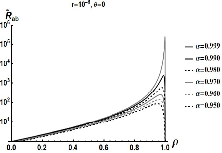
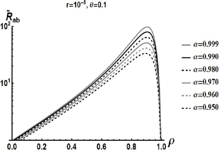
Figure 2: $\tilde{R}^{(mrr)}_{ab}=|\psi^{(2)}_{ab,mrr}(\omega)|^{2}=R^{(mrr)}_{ab}/|r_{ab}(\omega)|^{2}$ for $r=10^{-5}$ and (left) on mrr resonance $\theta=0$, (right) slightly off mrr resonance $\theta=0$, for $\alpha=(0.999,0.99,0.98,0.97,0.95,0.95)$.

Note that $\tilde{R}^{(mrr)}_{ab}$ is independent of the pump phase $\theta_{p}$ as can be observed from the overall factor of $e^{i\theta_{p}(\omega)}$ in Eq.(45). The surface of $\tilde{R}^{(mrr)}_{ab}\geq 1$ for resonance $\theta=0$ as a function of coupling $\rho$ and internal propagation loss $\alpha$ is plotted in Fig.(3). This plot indicates that strong biphoton pair production is favored by a high cavity Q ($\rho\rightarrow 1$), and low internal propagation loss ($\alpha\rightarrow 1$).

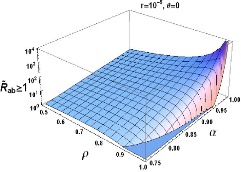
Figure 3: $\tilde{R}^{(mrr)}_{ab}=|\psi^{(2)}_{ab,mrr}(\omega)|^{2}$ for $r=10^{-5}$ on mrr resonance $\theta=0$ for $0.5\leq\rho\leq 1.0$ and $0.75\leq\alpha\leq 1.0$.

In Fig.(4) we plot $\tilde{R}^{(mrr)}_{ab}$ as a function of $\theta={\omega}\,T$ for $\rho=0.95$ and $\rho=0.50$, where the effect of the resonance structure of the mrr is manifest.

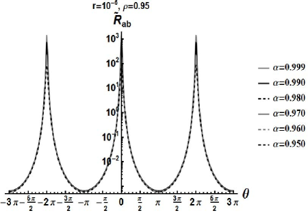
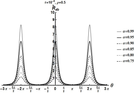
Figure 4: $\tilde{R}^{(mrr)}_{ab}=|\psi^{(2)}_{ab,mrr}(\omega)|^{2}$ for $r=10^{-5}$ and (left) $\rho=0.95$, and $\alpha=(0.999,0.99,0.98,0.97,0.95,0.95)$, and (right) (right) $\rho=0.5$ for $\alpha=(0.99,0.95,0.90,0.85,0.80,0.75)$

In the Appendix A we compare the expression for the biphoton generation rate in the high cavity Q limit with other expressions derived in the literature Scholz et al. (2009); Tsang (2011) using the standard Langevin approach.

The expressions for $R^{(mrr)}_{\textrm{CAR}}({\omega})$ in Eq.(42) and $R^{(mrr)}_{\textrm{herald}}({\omega})$ in Eq.(43) take on simple analytic forms given by

$$R^{(mrr)}_{\textrm{CAR}}({\omega})=\frac{\displaystyle\alpha_{a}^{2}\,\alpha_{b}^{2}\,\tau_{a}^{2}\,\tau_{a}^{2}\,}{\displaystyle(1-|r_{a}|^{2})\,\alpha_{b}^{2}\,\alpha_{b}^{2}+\alpha_{a}^{2}\,\left[(1-|r_{b}|^{2}-\alpha_{b}^{2})\tau_{a}^{2}-\alpha_{b}^{2}\,\alpha_{b}^{2}\right]}\rightarrow\frac{\displaystyle\alpha^{2}\,(1-\rho^{2})}{\displaystyle 2\,(1-|r|^{2}-\alpha^{2})},$$ (46)

were in the last expression we have again used $T_{a}=T_{b}=T$, $\rho_{a}=\rho_{b}=\rho$ and $\alpha_{a}=\alpha_{b}=\alpha$. Note $R^{(mrr)}_{\textrm{CAR}}({\omega})$ is independent of $\theta_{a},\,\theta_{b}$.

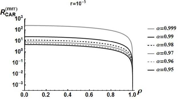
Figure 5: Coincidence to accidental rate $R^{(mrr)}_{\textrm{CAR}}({\omega})$ with $r=10^{-5}$ for $\alpha=(0.999,0.99,0.98,0.97,0.96,0.95)$.

In Fig.(5) we plot $R^{(mrr)}_{\textrm{CAR}}({\omega})$ with $r=10^{-5}$ for the operationally relevant (for $\alpha\leq 0.99$) internal propagation loss values $\alpha=(0.999,0.99,0.98,0.97,0.95,0.95)$.

The heralding efficiency $R^{(mrr)}_{\textrm{herald}}({\omega})$ takes even a simpler form, which again is independent of the phase accumulation angle $\theta_{b}$

$$R^{(mrr)}_{\textrm{herald}}({\omega})=\frac{\displaystyle\alpha_{b}^{2}\,(1-\rho_{b}^{2})}{\displaystyle(1-|r_{b}|^{2}-\alpha_{b}^{2}\,\rho_{b}^{2})}.$$ (47)

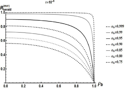
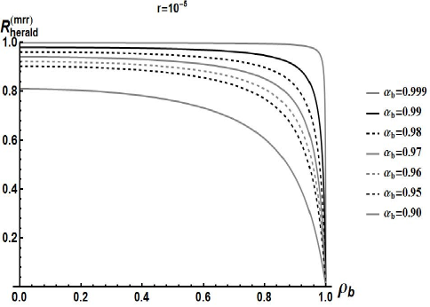
Figure 6: Heralding efficiency $R^{(mrr)}_{\textrm{herlad}}({\omega})$ with $r=10^{-5}$ for (left) $\alpha=(0.999,0.99,0.95,0.90,0.85,0.80,0.75)$. and the operationally relevant values (right) $\alpha=(0.999,0.99,0.98,0.97,0.95,0.95,0.90)$.

In Fig.(6) we plot $R^{(mrr)}_{\textrm{herald}}({\omega})$ with $r=10^{-5}$ for the internal propagation loss values (left) $\alpha~{}=~{}(0.99,0.95,0.90,$ $0.85,0.80,0.75)$, and for the operationally relevant (for $\alpha\leq 0.99$) internal propagation loss values $\alpha=(0.999,0.99,0.98,0.97,0.95,0.95,0.90)$. Even for high values of loss ($\alpha\leq 0.95$), the heralding efficiencies remain relatively high over a broad range of the coupling parameter $\rho_{b}$.

V Summary and Discussion

In this work we have investigated photon pair generation via SPDC and SFWM in a single bus microring resonator using a formalism that explicitly takes into account the round trip circulation of the fields inside the cavity. We investigated the biphoton generation-, coincidence to accidental, and heralding efficiency rates as function of the bus-mrr coupling loss $\rho=e^{-\gamma\,T\,/2}$ and internal propagation loss $\alpha=e^{-\gamma^{\prime}\,T\,/2}$ at rates $\gamma$ and $\gamma^{\prime}$, respectively (with $T$ the roundtrip circulation time of the field(s)). We showed Eq.(21) that the signal-idler output fields $\vec{a}_{out}({\omega})$ can be expressed in terms of the input fields $\vec{a}_{in}({\omega})$ and quantum noise operators $\vec{f}({\omega})$ as $\vec{a}_{out}({\omega})=G({\omega})\,\vec{a}_{in}({\omega})+H({\omega})\,\vec{f}({\omega})$. The matrix $G({\omega})$ encodes the classical phenomenological loss (for $\alpha<1$) Yariv (2000); Rabus (2007) of the mrr, while the matrix $H({\omega})$ incorporates the coupling and internal propagation loss due to the quantum Langevin noise fields $\vec{f}({\omega})$ required to preserve unitarity of the composite system (signal-idler) and environment (noise) structure. While the standard Langevin input-output formalism often used in the literature is valid in the high cavity Q limit ($\rho\approx 1-\gamma\,T/2\rightarrow 1,\,{\omega}\,T\ll 1$), and near cavity resonances, the formulation developed here is valid throughout the free spectral range of the mrr. We explored values of the noise field commutators which were uniquely derived by invoking the unitarity of the input and output fields (which required the later’s commutators to have the canonical form for free fields). For unequal signal and idler group velocities the cross noise commutators were non-zero, while in general, the noise commutators contained pump dependent contributions.

This work purposely concentrated on the weak (undepleted) pump limit and perfect phase matching in order to focus on the influence of the mrr coupling $\rho$ and internal propagation loss $\alpha$ parameters. As indicated earlier in this work, non-zero phase matching can be straightforwardly included, which modifies the $G$ and $H$ matrices with multiplicative $\sin$c function contributions. Similarly, this work only included effects of dispersion through the mrr round trip times $T_{k}=L/v_{k}$ for $k\in\{a,b\}$ for the signal ($a$) and idler fields ($b$) with possibly different group velocities $v_{k}$. Expansion of the frequency dependent momentum vectors for the signal and idler fields about a central frequency could also be straightforwardly accommodated. A further logical extension of this work would be to consider the strong pump field regime in the spirit of the recent work by Vernon and Sipe Vernon and Sipe (2015b) where effects such as pump depletion, and self-phase and cross-phase modulation could be taken into account.

*

Appendix A The high cavity Q limit

A.1 The high Q limit and reduction to the standard Langevin input-output formalism for a single mrr field

Both Raymer and McKintrie Raymer and McKinstrie (2013) and Alsing et al. Alsing et al. (2017) considered the comparison of their formulations to the high Q limit. Raymer and McKintrie define the high Q limit through the physical conditions (see Raymer and McKinstrie (2013), Section III) (i) the cross coupling $\tau_{a}$ is very small so that the cavity storage time is long, (ii) the cavity round trip time $T_{a}$ is small compared to the duration of the input-field pulse i.e. ${\omega}\,T_{a}\ll 1$, and (iii) the input field is narrow band and thus well contained within a single FSR of the mrr. By defining (now including internal loss)

$$\rho_{a} \equiv e^{-{\gamma}_{a}T_{a}/2}\approx 1-{\gamma}_{a}T_{a}/2,\qquad\tau_{a}=\sqrt{1-\rho_{a}^{2}}\approx\sqrt{{\gamma}_{a}T_{a}},$$

$$\alpha_{a} = e^{-{\gamma}^{\prime}_{a}T_{a}/2}\approx 1-{\gamma}^{\prime}_{a}T_{a}/2,\qquad e^{i\,{\omega}\,T_{a}}\approx 1+i\,{\omega}\,T_{a},$$ (48)

one has from Eq.(8)

$$G_{out,in}({\omega}) = \left(\frac{\rho_{a}-\alpha_{a}\,e^{i\theta_{a}}}{1-\rho_{a}\,\alpha_{a}\,e^{i\theta_{a}}}\right)\quad\hbox{ \raise-5.69054pt\hbox{$\textstyle{\longrightarrow}\atop\scriptstyle{\textrm{high Q}}$} }\quad\frac{i{\omega}+({\gamma}_{a}-{\gamma}^{\prime}_{a})/2}{-i{\omega}+({\gamma}_{a}+{\gamma}^{\prime}_{a})/2},$$ (49a)

$$H_{out,in}({\omega})\equiv|H_{out,in}({\omega})| = \frac{|\tau_{a}|^{2}\,(1-\alpha_{a}^{2})}{|1-\rho_{a}\,\alpha_{a}\,e^{i\,\theta_{a}}|^{2}}\;\quad\hbox{ \raise-5.69054pt\hbox{$\textstyle{\longrightarrow}\atop\scriptstyle{\textrm{high Q}}$} }\quad\frac{\sqrt{{\gamma}_{a}\,{\gamma}^{\prime}_{a}}}{{\omega}^{2}+[({\gamma}_{a}+{\gamma}^{\prime}_{a})/2]^{2}},$$ (49b)

where, without loss of generality, we have taken the phase of $H_{out,in}({\omega})$ to be zero (or equivalently, absorbed into the definition of the noise operator $f_{a}({\omega})$).

Under the assumptions of the high cavity Q limit one has $a(L_{-},t)\approx a(0_{+},t)$. Raymer and McKinstrie Raymer and McKinstrie (2013) show that by defining the rescaled cavity field as $a(t)\equiv\sqrt{T_{a}}\,a(0_{+},t)$ and considering the transfer function $G_{0_{+},in}(t)$ in the time domain, the equation of motion (without noise) becomes $\partial_{t}\,a(t)=-\frac{1}{2}{\gamma}^{\prime}_{a}\,a(t)+\sqrt{{\gamma}^{\prime}_{a}}\,a_{int}(t)$. Additionally, the output boundary condition Eq.(2b), in the limit $\rho_{a}\rightarrow 1$, $\tau_{a}\rightarrow\sqrt{{\gamma}^{\prime}_{a}\,T_{a}}$ becomes $a_{out}(t)=\sqrt{{\gamma}^{\prime}_{a}}\,a(t)-a_{in}$, which is the standard Langevin boundary condition $a_{in}+a_{out}=\sqrt{\gamma_{a}}\,a$ Walls and Milburn (1994); Orszag (2000).

A.2 The high cavity Q limit of $G({\omega})$ and $H({\omega})$

The high cavity Q limit is defined by (see Raymer and McKinstrie Raymer and McKinstrie (2013)) $\rho_{k}\equiv e^{-\gamma_{k}\,T_{k}/2}\approx 1-\gamma_{k}\,T_{k}/2$ for $k\in\{a,b\}$ which implies $\tau_{k}^{2}\approx\gamma_{k}\,T_{k}$, and by taking the limit ${\omega}\,T_{k}\ll 1$ so that $e^{i\theta_{k}}\approx 1+i\,{\omega}\,T_{k}$. If we further assume that the internal propagation loss is small we can also take $\alpha_{k}\approx 1-\gamma^{\prime}_{k}\,T_{k}/2$. We then have $S_{k}=(1-\rho_{k}\alpha_{k}\,e^{i\,\theta_{k}})^{-1}\approx[(s+{\Gamma}_{k}/2)\,T_{k}]^{-1}$, a complex Lorentzian lineshape factor, where for simplicity we have defined $s\equiv-i{\omega}$ ($s$ can be considered as a Laplace transform solution variable), and have defined the total decay rate ${\Gamma}_{k}=\gamma_{k}+\gamma^{\prime}_{k}$. Let us also further define $\Delta_{k}=\gamma_{k}-\gamma^{\prime}_{k}$ as the difference between the coupling and internal propagation losses. Then, $e^{i\xi_{k}L}-\rho_{k}\rightarrow(-s+\Delta_{k}/2)\,T_{k}$ and $D(s)\approx\left[(s+{\Gamma}_{a}/2)\,(s+{\Gamma}_{b}/2)-|g\alpha_{p}|^{2}\right]\,T_{a}\,T_{b}\equiv\tilde{D}(s)\,T_{a}\,T_{b}$. We then obtain from Eq.(22f)

$$G({\omega})\hbox{ \raise-5.69054pt\hbox{$\textstyle{\longrightarrow}\atop\scriptstyle{\textrm{high Q}}$} }$$

$$\frac{1}{\tilde{D}(s)}\,\left(\begin{array}[]{cc}(-s+\Delta_{a}/2)\,(s+{\Gamma}_{b}/2)+|g\alpha_{p}|^{2}\,[1-\gamma_{a}\,T_{a}/2]&i\,g\,\alpha_{p}\,\sqrt{\gamma_{a}\,\gamma_{b}}\,\sqrt{T_{b}/T_{a}}\,[1-(s+{\gamma}^{\prime}_{b}/2)\,T_{b}]\\ -i\,g\,\alpha^{*}_{p}\,\sqrt{\gamma_{a}\,\gamma_{b}}\,\sqrt{T_{a}/T_{b}}\,[1-(s+{\gamma}^{\prime}_{a}/2)\,T_{a}]&(-s+\Delta_{b}/2)\,(s+{\Gamma}_{a}/2)+|g\alpha_{p}|^{2}\,[1-\gamma_{b}\,T_{b}/2],\end{array}\right).\qquad\;\;$$ (52)

For the noise terms, let us redefine the noise operators as $\tilde{f}_{k}({\omega})\equiv(1-\alpha_{k}^{2})^{-1/2}\,f_{k}({\omega})$ for $k\in\{a,b\}$ and equivalently the values of the commutators as $[f_{k}({\omega}),f^{\dagger}_{k}({\omega})]=C_{kk}({\omega})\equiv(1-\alpha_{k}^{2})\,\tilde{C}_{kk}({\omega})$ and $D_{ab}({\omega})\equiv(1-\alpha_{a}^{2})^{1/2}\,(1-\alpha_{b}^{2})^{1/2}\tilde{D}_{ab}({\omega})$, so that $[\tilde{f}_{k}({\omega}),\tilde{f}_{k}({\omega}^{\prime})]=\tilde{C}_{kk}({\omega})\,\delta({\omega}-{\omega}^{\prime})$ and $[\tilde{f}_{a}({\omega}),\tilde{f}_{b}({\omega}^{\prime})]=\tilde{D}_{ab}({\omega})\,\delta({\omega}-{\omega}^{\prime})$. Then

$$\vec{a}_{out}\equiv G({\omega})\,\vec{a}_{in}+\tilde{H}({\omega})\,\vec{\tilde{f}}({\omega}),\quad\tilde{H}({\omega})\,=H({\omega})\,\Lambda_{\alpha},\quad\Lambda_{\alpha}\equiv\left(\begin{array}[]{cc}(1-\alpha_{a}^{2})^{1/2}&0\\ 0&(1-\alpha_{b}^{2})^{1/2}\\ \end{array}\right).$$ (53)

From Eq.(24) and Eq.(53) in the high Q limit, where $(1-\alpha^{2}_{k})^{1/2}\rightarrow\sqrt{{\gamma}^{\prime}_{k}\,T_{k}}$, we then have

$$\tilde{H}({\omega})\hbox{ \raise-5.69054pt\hbox{$\textstyle{\longrightarrow}\atop\scriptstyle{\textrm{high Q}}$} }\frac{1}{\tilde{D}(s)}\,\left(\begin{array}[]{cc}\sqrt{\gamma_{a}\,\gamma^{\prime}_{a}}\,(s+{\Gamma}_{b}/2)&i\,g\,\alpha_{p}\,\sqrt{\gamma_{a}\,\gamma^{\prime}_{b}}\,\sqrt{T_{b}/T_{a}}\\ -i\,g\,\alpha^{*}_{p}\,\sqrt{\gamma^{\prime}_{a}\,\gamma_{b}}\,\sqrt{T_{a}/T_{b}}&\sqrt{\gamma_{b}\,\gamma^{\prime}_{b}}\,(s+{\Gamma}_{a}/2),\end{array}\right).\qquad\;\;$$ (54)

Except for the extra correction factors indicated in the square brackets in $G({\omega})$ (which can be safely approximated as unity to lowest order in $|g\,\alpha_{p}|$) these matrices are the same expressions as obtained by Tsang (see (4.11) in Tsang (2011)) using the standard Langevin input/output procedure and assuming $T_{a}=T_{b}=L/v$.

Note further that to zeroth order in $|g\alpha_{p}|$ we have $D^{-1}\approx S_{a}\,S_{b}/(T_{a}\,T_{b})\rightarrow[(s+{\Gamma}_{a}/2)^{-1}\,(s+{\Gamma}_{b}/2)\,T_{a}\,T_{b}]^{-1}$ and thus $G({\omega})$ reduces in first order in $|g\alpha_{p}|$ to

$$G({\omega})\hbox{ \raise-5.69054pt\hbox{$\textstyle{\longrightarrow}\atop\scriptstyle{\stackrel{{\scriptstyle\textrm{\scriptsize high Q}}}{{\mathcal{O}(|g\,\alpha_{p}|)}}}$} }\left(\begin{array}[]{cc}\frac{\displaystyle-s+\Delta_{a}/2}{\displaystyle s+{\Gamma}_{a}/2}&i\,g\,\alpha_{p}\,\left(\frac{\displaystyle\sqrt{\gamma_{a}}}{\displaystyle s+{\Gamma}_{a}/2}\right)\,\left(\frac{\displaystyle\sqrt{\gamma_{b}}}{\displaystyle s+{\Gamma}_{b}/2}\right)\\ -i\,g\,\alpha^{*}_{p}\,\left(\frac{\displaystyle\sqrt{\gamma_{a}}}{\displaystyle s+{\Gamma}_{a}/2}\right)\,\left(\frac{\displaystyle\sqrt{\gamma_{b}}}{\displaystyle s+{\Gamma}_{b}/2}\right)&\frac{\displaystyle-s+\Delta_{b}/2}{\displaystyle s+{\Gamma}_{b}/2},\end{array}\right),\qquad\;\;$$ (55)

where we have also used $e^{i\xi_{k}L}\approx 1$. In this limit, the diagonal terms $G_{kk}$, which directly couple $(\vec{a}_{out})_{k}$ to $(\vec{a}_{in})_{k}$ for $k\in\{a,b\}$, have same frequency dependent shifts of the output signal-idler fields relative to the internal signal-idler fields as given by the conventional Langevin approach Haus (1984); Walls and Milburn (1994); Orszag (2000). The lower order (in $|g\,\alpha_{p}|$) off diagonal terms $G_{ab}$ and $G_{ba}$ contain the product of Lorentzian lineshape factors $\sqrt{\gamma_{k}}/(s+{\Gamma}_{k}/2)$ relating the output signal-idler fields to the opposite idler/signal fields inside the cavity. Similarly, for $\tilde{H}({\omega})$ we have

$$\tilde{H}({\omega})\hbox{ \raise-5.69054pt\hbox{$\textstyle{\longrightarrow}\atop\scriptstyle{\stackrel{{\scriptstyle\textrm{\scriptsize high Q}}}{{\mathcal{O}(|g\,\alpha_{p}|)}}}$} }\left(\begin{array}[]{cc}\frac{\displaystyle\sqrt{{\gamma}_{a}\,{\gamma}^{\prime}_{a}}}{\displaystyle s+{\Gamma}_{a}/2}&\frac{\displaystyle i\,g\,\alpha_{p}\,\sqrt{{\gamma}_{a}\,{\gamma}^{\prime}_{b}}}{\displaystyle(s+{\Gamma}_{a}/2)\,(s+{\Gamma}_{b}/2)}\\ \frac{\displaystyle i\,g\,\alpha^{*}_{p}\,\sqrt{{\gamma}^{\prime}_{a}\,{\gamma}_{b}}}{\displaystyle(s+{\Gamma}_{a}/2)\,(s+{\Gamma}_{b}/2)}&\frac{\displaystyle\sqrt{{\gamma}_{b}\,{\gamma}^{\prime}_{b}}}{\displaystyle s+{\Gamma}_{b}/2}\end{array}\right).$$ (56)

A.3 Biphoton generation rate $R_{ab}({\omega})$ in the high $Q$ limit

To make connection with other works, let us more closely examine the two-photon generation rate given by $R_{ab}({\omega})=|r_{ab}(\omega)|^{2}\,|\psi^{(2)}_{ab}({\omega})|^{2}$ in the high cavity Q limit. Note that from Eq.(23a) we can write the $D(s)$ in Eq.(39c) and Eq.(40e) as $D(s)=(1-\rho_{a}\,\alpha_{a}\,e^{-s\,T_{a}})\,(1-\rho_{b}\,\alpha_{b}\,e^{-s\,T_{b}})-|g\,\alpha_{p}|^{2}\,T_{a}\,T_{b}$ where $s=-i\,{\omega}$. The pole structure of $D(s)$ is obtained by the roots $s_{\pm}$ of $D(s_{\pm})=0$. In general this is a transcendental equation which must be solved numerically. If we approximate $e^{-s\,T_{k}}\approx 1-s\,T_{k}$, we obtain a quadratic equation in $s$ with poles $s_{\pm}$, and

$$D(s) \approx (s-s_{+})\,(s-s_{-}),$$

$$s_{\pm} = \frac{1}{2}\,\left(\frac{\displaystyle y_{a}}{\displaystyle x_{a}}+\frac{\displaystyle y_{b}}{\displaystyle x_{b}}\right)\pm\sqrt{\left[\frac{1}{2}\,\left(\frac{\displaystyle y_{a}}{\displaystyle x_{a}}-\frac{\displaystyle y_{b}}{\displaystyle x_{b}}\right)\right]^{2}+|g\,\alpha_{p}|^{2}},\quad x_{k}=\rho_{k}\,\alpha_{k},\quad y_{k}=\frac{\displaystyle(1-\rho_{k}\,\alpha_{k})}{\displaystyle T_{k}},\qquad\quad$$ (57a)

$$\textstyle{\longrightarrow}\atop\scriptstyle{\textrm{high Q}} \left(\frac{\displaystyle{\Gamma}_{a}+{\Gamma}_{b}}{\displaystyle 4}\right)\pm\sqrt{\left(\frac{\displaystyle{\Gamma}_{a}-{\Gamma}_{b}}{\displaystyle 4}\right)^{2}+|g\,\alpha_{p}|^{2}}\;\equiv\;\pi_{\pm},$$ (57b)

$$\textstyle{\longrightarrow}\atop\scriptstyle{\stackrel{{\scriptstyle\textrm{\scriptsize high Q}}}{{\mathcal{O}(|g\,\alpha_{p}|)}}} \left\{\begin{array}[]{c}-{\Gamma}_{a}/2\\ -{\Gamma}_{b}/2\end{array}\right.\quad\textrm{for}\quad{\Gamma}_{b}>{\Gamma}_{a},$$ (57e)

where $\pi_{\pm}$ are the poles of $D(s)$ as computed by Tsang Tsang (2011) using a standard Langevin input-output calculation. Then, the two-photon generation rate becomes to lowest order in $|g\,\alpha_{p}|^{2}$

$$R_{ab}({\omega}) = |r_{ab}(\omega)|^{2}\,|\psi^{(2)}_{ab}({\omega})|^{2}\approx|r_{ab}(\omega)|^{2}\,|G^{(L)*}_{aa}({\omega})\,G^{(L)}_{bb}({\omega})|^{2},$$ (58a)

$$\textstyle{\longrightarrow}\atop\scriptstyle{D(s)\approx(s-s_{+})\,(s-s_{-})} |g\,\alpha_{p}|^{2}\,\frac{\displaystyle\left(\frac{\tau_{a}}{\sqrt{T_{a}}}\right)^{2}\,\left|\frac{1-\rho_{b}\,e^{i\xi_{b}L}}{T_{b}}\right|^{2}\,\left|e^{i\xi_{a}L}\right|^{2}}{\displaystyle({\omega}^{2}+s^{2}_{+})\,({\omega}^{2}+s^{2}_{-})}\cdot\frac{\displaystyle\left(\frac{\tau_{b}}{\sqrt{T_{b}}}\right)^{2}\,\left|\frac{1-\rho_{a}\,e^{i\xi_{b}L}}{T_{a}}\right|^{2}\,\left|e^{i\xi_{b}L}\right|^{2}}{\displaystyle({\omega}^{2}+s^{2}_{+})\,({\omega}^{2}+s^{2}_{-})},\qquad\;\;\;$$

$$\textstyle{\longrightarrow}\atop\scriptstyle{\textrm{high Q}} |g\,\alpha_{p}|^{2}\,\frac{\displaystyle{\gamma}_{a}\,\left[{\omega}^{2}+({\Gamma}_{b}/2)^{2}\right]}{\displaystyle({\omega}^{2}+s^{2}_{+})\,({\omega}^{2}+s^{2}_{-})}\cdot\frac{\displaystyle{\gamma}_{b}\,\left[{\omega}^{2}+({\Gamma}_{a}/2)^{2}\right]}{\displaystyle({\omega}^{2}+s^{2}_{+})\,({\omega}^{2}+s^{2}_{-})},$$ (58b)

$$\textstyle{\longrightarrow}\atop\scriptstyle{\stackrel{{\scriptstyle\textrm{\scriptsize high Q}}}{{\mathcal{O}(|g\,\alpha_{p}|^{2})}}} |g\,\alpha_{p}|^{2}\,\frac{\displaystyle{\gamma}_{a}}{\displaystyle[{\omega}^{2}+({\Gamma}_{a}/2)^{2}]}\cdot\frac{\displaystyle{\gamma}_{b}}{\displaystyle[{\omega}^{2}+({\Gamma}_{b}/2)^{2}]},$$ (58c)

where in the third line we have used $|e^{i\xi_{k}L}|^{2}\approx 1$ and in the fourth line we have used Eq.(57e). The above expressions generalize two photon rate $R_{ab}({\omega})=|g\,\alpha_{p}|^{2}\,{\gamma}_{a}\,{\gamma}_{b}/[({\omega}^{2}+s^{2}_{+})\,({\omega}^{2}+s^{2}_{-})]$ computed by Tsang Tsang (2011), which to $\mathcal{O}(|g\,\alpha_{p}|^{2})$ agrees with Eq.(58b). The last line Eq.(58c) is the form computed by Scholz using the (complex) Lorenztian modified form $\sqrt{\gamma_{a}}\,a({\omega})/(s+{\Gamma}_{a}/2)$ and $\sqrt{\gamma_{b}}\,b^{\dagger}({\omega})/(-s+{\Gamma}_{b}/2)$ for the field operators inside the mrr. The expression Eq.(58a), quadratic in the poles $s_{\pm}$, more fully takes into account the effect of the the field circulation factors $S_{k}=1/[1-\rho_{k}\,e^{i\xi_{b}L}]$ on the two-photon generation rate.