Fingerprints of angulon instabilities in the spectra of matrix-isolated molecules

Abstract

The formation of vortices is usually considered to be the main mechanism of angular momentum disposal in superfluids. Recently, it was predicted that a superfluid can acquire angular momentum via an alternative, microscopic route – namely, through interaction with rotating impurities, forming so-called ‘angulon quasiparticles’ [Phys. Rev. Lett. 114, 203001 (2015)]. The angulon instabilities correspond to transfer of a small number of angular momentum quanta from the impurity to the superfluid, as opposed to vortex instabilities, where angular momentum is quantized in units of $\hbar$ per atom. Furthermore, since conventional impurities (such as molecules) represent three-dimensional (3D) rotors, the angular momentum transferred is intrinsically 3D as well, as opposed to a merely planar rotation which is inherent to vortices. Herein we show that the angulon theory can explain the anomalous broadening of the spectroscopic lines observed for CH₃ and NH₃ molecules in superfluid helium nanodroplets, thereby providing a fingerprint of the emerging angulon instabilities in experiment.

One of the distinct features of the superfluid phase is the formation of vortices – topological defects carrying quantized angular momentum, which arise if the bulk of the superfluid rotates faster than some critical angular velocity Pitaevskii and Stringari (2016); Leggett (2006). Vortex nucleation has been considered to be the main mechanism angular momentum disposal in superfluids Pitaevskii and Stringari (2016); Pethick and Smith (2008); Leggett (2006); Gomez, Loginov, and Vilesov (2012); Gomez et al. (2014). Recently, it was predicted that a superfluid can acquire angular momentum via a different, microscopic route, which takes effect in the presence of rotating impurities, such as molecules Toennies and Vilesov (2004, 1998); Callegari et al. (2001); Stienkemeier and Lehmann (2006); Choi et al. (2006); Szalewicz (2008); Hartmann et al. (1995); Kwon et al. (2000). In particular, it was demonstrated that a rotating impurity immersed in a superfluid forms the ‘angulon’ quasiparticle, which can be thought of as a rigid rotor dressed by a cloud of superfluid excitations carrying angular momentum Schmidt and Lemeshko (2015, 2016); Lemeshko and Schmidt (2017); Redchenko and Lemeshko (2016); Li, Seiringer, and Lemeshko (2016); Midya et al. (2016); Yakaboylu and Lemeshko (2017); Bighin and Lemeshko (2017).

The angulon theory was able to describe, in good agreement with experiment, renormalization of rotational constants Lemeshko (2017); Shchadilova (2017) and laser-induced dynamics Shepperson et al. (2017a, b) of molecules in superfluid helium nanodroplets. One of the key predictions of the angulon theory are the so-called ‘angulon instabilities’ Schmidt and Lemeshko (2015, 2016); Lemeshko and Schmidt (2017) that occur at some critical value of the molecule-superfluid coupling where the angulon quasiparticle becomes unstable and one or a few quanta of angular momentum are resonantly transferred from the impurity to the superfluid. These instabilities are fundamentally different from the vortex instabilities, associated with the transfer of angular momentum quantised in units of $\hbar$ per atom of the superfluid. Furthermore, vortices can be thought of as planar rotors, i.e., the eigenstates of the $\hat{L}_{z}$ operator. Angulons, on the other hand, are the eigenstates of the total angular momentum operator, $\hat{\mathbf{L}}^{2}$, and therefore the transferred angular momentum is three-dimensional. While vortex instabilities have been subject to several experimental studies in the context of superfluid helium Blaauwgeers et al. (2000); Bewley, Lathrop, and Sreenivasan (2006); Gomez, Loginov, and Vilesov (2012); Zmeev et al. (2013); Gomez et al. (2014); Spence et al. (2014); Thaler et al. (2014); Jones et al. (2016), ultracold quantum gases Matthews et al. (1999); Burger et al. (2001); Zwierlein et al. (2005, 2005); Lin et al. (2009); Freilich et al. (2010), and superconductors Harada et al. (1992, 1996); Wallraff et al. (2003); Guillamon et al. (2009), the transfer of angular momentum to a superfluid via the angulon instabilities has not yet been observed in experiment.

In this Letter we provide evidence for the emergence of the angulon instabilities in experiments on CH₃ Morrison, Raston, and Douberly (2013) and NH₃ Slipchenko and Vilesov (2005) molecules trapped in superfluid helium nanodroplets. Spectroscopy of molecules matrix-isolated in ⁴He has been an active area of research during the last two decades Toennies and Vilesov (2004, 1998); Callegari et al. (2001); Stienkemeier and Lehmann (2006); Choi et al. (2006); Szalewicz (2008); Hartmann et al. (1995); Kwon et al. (2000); Mudrich and Stienkemeier (2014). In general, it is believed that the superfluid helium environment alters the molecular rovibrational spectra only weakly, the main effect being the renormalization of the molecular moment of inertia Toennies and Vilesov (2004), which is somewhat analogous to the renormalization of effective mass of electrons propagating in crystals Lemeshko (2017). It has been shown, however, that superfluid ⁴He leads to homogeneous broadening of some spectroscopic lines. While the inhomogeneous line broadening is known to arise due to the size distribution of the droplets Toennies and Vilesov (2004), the mechanisms of the homogeneous broadening have been under active discussion Hartmann et al. (1995); Callegari et al. (2001); Slipchenko and Vilesov (2005); Scheele et al. (2005); Morrison, Raston, and Douberly (2013); Ravi et al. (2011); Merritt, Douberly, and Miller (2004); Hartmann et al. (1996); Nauta and Miller (1999, 2000, 2001); Slenczka et al. (2001); Zillich and Whaley (2010); Von Haeften et al. (2006); Zillich, Whaley, and von Haeften (2008); von Haeften et al. (2006); Zillich, Whaley, and von Haeften (2008); Zillich, Kwon, and Whaley (2004); Zillich and Whaley (2004, 2007); Moore and Miller (2003); Gutberlet, Schwaab, and Havenith (2011); Lehmann (2007); Rudolph et al. (2007); Skvortsov et al. (2009); Pentlehner et al. (2010); Hoshina et al. (2010); Zhang and Drabbels (2014) and their convincing microscopic interpretation has been wanting.

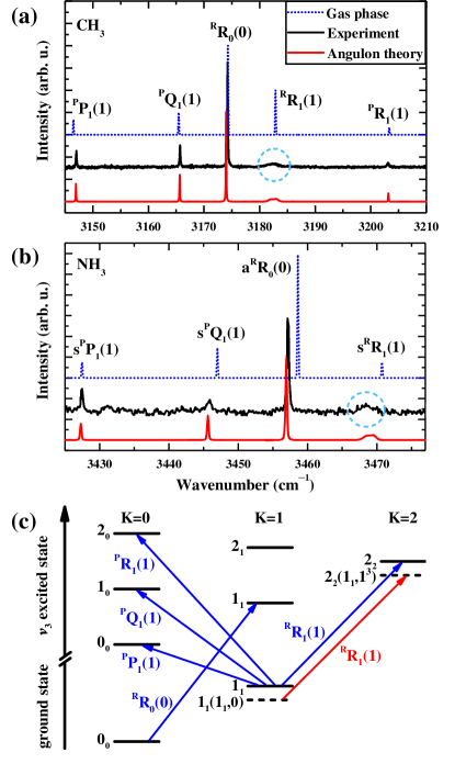
Figure 1: (a) $\nu_{3}$ ro-vibrational spectrum of CH₃: gase phase simulation (dashed blue) and experiment in superfluid helium nanodroplets (black) in comparison with the angulon theory (red). (b) Same as (a) for NH₃. (c) Schematics of relevant gas-phase molecular levels (black solid lines) and the corresponding spectroscopic transitions (blue arrows). The case of NH₃ involves additional inversion doubling of the levels, which is not shown Ruzi and Anderson (2013). In the presence of helium, the $\mathrm{{}^{R}R}_{1}(1)$ transition (red line) takes place between the angulon states, $1_{1}(1_{1},0)$ and $2_{2}(1_{1},1^{3})$ (dashed lines), which results in the line broadening encircled in (a) and (b). Experimental data adapted with permission from Refs. Morrison, Raston, and Douberly (2013); Slipchenko and Vilesov (2005).

Our aim here is to explain the anomalously large broadening of the $\mathrm{{}^{R}R_{1}(1)}$ transition, recently observed in in $\nu_{3}$ rovibrational spectra of CH₃ in helium droplets Morrison, Raston, and Douberly (2013). The experimental spectrum is shown in Fig. 1(a) by the black solid line; Fig. 1(c) provides a schematic illustration of the molecular levels in the gas phase. One can see that all the spectroscopic lines are left intact by the helium environment, except the $\mathrm{{}^{R}R_{1}(1)}$ line, which is broadened by $\sim 50$ GHz sup compared to the gas-phase simulation (blue dots). In Ref. Morrison, Raston, and Douberly (2013) this feature was qualitatively explained by the coupling between the $2_{2}$ and $1_{1}$ molecular levels induced by the $V_{33}(r)$ anisotropic term of the CH₃–He potential energy surface (PES) sup , based on the theory of Ref. Zillich and Whaley (2010). A similar effect was also present in earlier experiments on NH₃ Slipchenko and Vilesov (2005), see Fig. 1(b). Our goal is to provide a microscopic description of the spectra shown using the angulon theory and thereby demonstrate that the broadening is due to an angulon instability, accompanied by a resonant transfer of $3\hbar$ of angular momentum from the molecule to the superfluid. It is important to note that the angulon quasiparticle theory described below is substantially simpler – and therefore more transparent – than numerical calculations based on Monte-Carlo algorithms Zillich, Whaley, and von Haeften (2008); von Haeften et al. (2006); Zillich, Whaley, and von Haeften (2008); Zillich, Kwon, and Whaley (2004); Zillich and Whaley (2004, 2007, 2010); Moroni, Blinov, and Roy (2004); Moroni et al. (2003); Paesani et al. (2003); Blinov, Song, and Roy (2004); Miura (2007); Skrbic, Moroni, and Baroni (2007); Paesani, Kwon, and Whaley (2005); Paolini et al. (2005); Markovskiy and Mak (2009); Wang et al. (2011); Rodriguez-Cantano et al. (2013).

We start by generalizing the angulon Hamiltonian, derived in Refs. Schmidt and Lemeshko (2015); Lemeshko and Schmidt (2017) for linear-rotor molecules, to the case of symmetric tops such as CH₃ and NH₃ sup :

$$\begin{split}&\hat{H}=B\bm{\hat{\mathrm{J}}^{2}}+(C-B)\hat{J}^{\prime 2}_{z}+\sum_{q\lambda\mu}\omega(q)\hat{b}^{{\dagger}}_{q\lambda\mu}\hat{b}_{q\lambda\mu}+\\ +\alpha\sum_{q\lambda\mu\xi}&v_{\lambda\xi}(q)\bigg{(}\hat{b}^{\dagger}_{q\lambda\mu}[D^{\lambda}_{\mu\xi}(\hat{\Omega})+(-1)^{\xi}D^{\lambda}_{\mu-\xi}(\hat{\Omega})]+\text{h.c.}\bigg{)}\end{split}$$ (1)

where we introduced the notation $\sum_{q}\equiv\int dq$ and set $\hbar\equiv 1$. The first two terms of Eq. (LABEL:eq:hamil) correspond to the kinetic energy of a symmetric-top impurity, with $\mathbf{\hat{J}}$ and $\mathbf{\hat{J^{\prime}}}$ the angular momentum operators acting in the laboratory and impurity frames, respectively Herzberg (1945); Bernath (2005); Bunker and Jensen (2006); Lefebvre-Brion and Field (2004). $B$ and $C$ are rotational constants determined by the corresponding moments of inertia as $B=\frac{1}{2I_{x^{\prime}}}=\frac{1}{2I_{y^{\prime}}}$ and $C=\frac{1}{2I_{z^{\prime}}}$. The energies of the free impurity states are given by $E_{JK}=BJ(J+1)+(C-B)K^{2}$, and correspond to $(2J+1)$–fold degenerate states, $|JMK\rangle$. Here $J$ is the angular momentum of the molecule, $M$ gives its projection on the $z$-axis of the laboratory frame, and $K$ gives its projection on the $z^{\prime}$-axis of the molecular frame.

The third term of the Hamiltonian represents the kinetic energy of the bosons in the superfluid, as given by the dispersion relation, $\omega(q)$. Here the boson creation and annihilation operators, $\hat{b}^{{\dagger}}_{q\lambda\mu}$ and $\hat{b}_{q\lambda\mu}$, are expressed in the angular momentum basis, where $q=|\bm{\mathrm{q}}|$ labels the boson’s linear momentum, $\lambda$ is the angular momentum, and $\mu$ is the angular momentum projection onto the $z$-axis, see Ref. Lemeshko and Schmidt (2017) for details.

The last term of Eq. (LABEL:eq:hamil) defines the interactions between the molecular impurity and the superfluid, where we have introduced an auxiliary parameter $\alpha$, which for comparison with experiment will be set to $\alpha\equiv 1$. $D^{\lambda}_{\mu\xi}(\hat{\Omega})$ are Wigner $D$-matrices, and $\hat{\Omega}\equiv(\hat{\theta},\hat{\phi},\hat{\gamma})$ are the angle operators defining the orientation of the molecular axis in the laboratory frame. It is important to note that Eq. (LABEL:eq:hamil) becomes quantitatively accurate for a symmetric-top molecule immersed in a weakly-interacting Bose-Einstein Condensate Schmidt and Lemeshko (2015); Lemeshko and Schmidt (2017). It has been demonstrated, however, that one can develop a phenomenological theory based on the angulon Hamiltonian that describes rotations of molecules in superfluid ⁴He in good agreement with experiment Lemeshko (2017); Shepperson et al. (2017a). Here we pursue a similar route, i.e., we fix the interaction parameters, $v_{\lambda\xi}(q)$, based on ab inito PES’s sup ; Meyer et al. (1986); Hodges and Wheatley (2001); Dagdigian and Alexander (2011); Suarez et al. (2011); Green (1976, 1980) in such a way that the depth of the trapping potential (mean-field energy shift) for the molecule is reproduced Toennies and Vilesov (2004).

Let us proceed with calculating the spectrum of a symmetric-top impurity in ⁴He in the weakly-interacting regime, applicable to both CH₃ and NH₃ Lemeshko (2017). We start from constructing a variational ansatz based on single-boson excitations, analogous to that used in Ref. Schmidt and Lemeshko (2015) for linear molecules:

$$\begin{split}|\psi_{LMk_{0}}\rangle=Z^{1/2}_{LMk_{0}}&|0\rangle|LMk_{0}\rangle+\\ &+\sum_{\begin{subarray}{k}q\lambda\mu\\ jmk\end{subarray}}\beta_{\lambda jk}(q)C^{LM}_{jm,\lambda\mu}\hat{b}^{{\dagger}}_{q\lambda\mu}|0\rangle|jmk\rangle\end{split}$$ (2)

Here $|0\rangle$ is the vacuum of bosonic excitations, and $Z^{1/2}_{LMk_{0}}$ and $\beta_{\lambda jk}(q)$ are the variational parameters obeying the normalization condition, $Z_{LMk_{0}}=1-\sum_{q\lambda jk}|\beta_{\lambda jk}(q)|^{2}$. The coefficient $Z_{LMk_{0}}$ is the so-called quasiparticle weight Lifshitz and Pitaevskii (1980); Altland and Simons (2010), i.e., the overlap between the dressed angulon state, $|\psi_{LMk_{0}}\rangle$, and the free molecular state, $|LMk_{0}\rangle|0\rangle$.

The angulon state (2) is an eigenstate of the total angular momentum operators, $\mathbf{\hat{L}}^{2}$ and $\hat{L}_{z}$, which correspond to good quantum numbers $L$ and $M$. In the absence of external fields, the quantum number $M$ is irrelevant and will be omitted hereafter. In addition, we introduce approximate quantum numbers $j$ and $k$, describing the angular momentum of the molecule and its projection on the molecular axis $z^{\prime}$ ($k=k_{0}$ for $j=L$), and $\lambda$ giving angular momentum of the excited boson. The idea of approximate quantum numbers in the present context is analogous to (and inspired by) Hund’s cases of molecular spectroscopy Lefebvre-Brion and Field (2004). As a result, we can label the angulon states as $L_{k_{0}}(j_{k},N_{\lambda}$${}^{\lambda})$, where $N_{\lambda}$ gives the number of phonons in a state with angular momentum $\lambda$. The ansatz of Eq. (2) restricts the possible values of $N_{\lambda}$ to 0 or 1.

After the minimization of the energy, $E=\langle\psi_{LMk_{0}}|\hat{H}|\psi_{LMk_{0}}\rangle/\langle\psi_{LMk_{0}}|\psi_{LMk_{0}}\rangle$, with respect to $Z^{1/2\ast}_{LMk_{0}}$ and $\beta_{\lambda jk}^{\ast}(q)$, we arrive to the Dyson-like equation Schmidt and Lemeshko (2015); Lemeshko and Schmidt (2017):

$$E=BL(L+1)+(C-B)k_{0}^{2}-\Sigma_{Lk_{0}}(E)$$ (3)

Here $\Sigma_{Lk_{0}}(E)$ is the angulon self-energy containing all the information about the molecule-helium interaction:

$$\begin{split}&\Sigma_{Lk_{0}}(E)=\sum_{q\lambda jk\xi\xi^{\prime}}\frac{v_{\lambda\xi}(q)v_{\lambda\xi^{\prime}}(q)}{Bj(j+1)+(C-B)k^{2}-E+\omega(q)}\times\\ \times(C&{}^{jk}_{LK,\lambda\xi}+(-1)^{\xi}C^{jk}_{LK,\lambda-\xi})(C^{jk}_{LK,\lambda\xi^{\prime}}+(-1)^{\xi^{\prime}}C^{jk}_{LK,\lambda-\xi^{\prime}})\end{split}$$ (4)

In the limit of $k=0,K=0$, $\xi=0$, and $\xi^{\prime}=0$, Eqs. (3) and (4) reduce to the equations derived in Ref. Schmidt and Lemeshko (2015) for a linear molecule.

Within the electric dipole approximation, the angulon excitation spectrum is given by the following expression:

$$\begin{split}S^{v^{\prime}v}_{LMk_{0}}(E)=|\langle v^{\prime}|\langle&\psi_{L^{\prime}M^{\prime}k_{0}^{\prime}}|\bm{\hat{\mu}}|\psi_{LMk_{0}}\rangle|v\rangle|^{2}\times\\ \times&\frac{\mathrm{Im}\Sigma_{L^{\prime}k_{0}^{\prime}}(E)}{(\gamma_{L^{\prime}k_{0}^{\prime}}(E)-E)^{2}+[\mathrm{Im}\Sigma_{L^{\prime}k_{0}^{\prime}}(E)]^{2}}\end{split}$$ (5)

where $\gamma_{L^{\prime}k_{0}^{\prime}}(E)=BL^{\prime}(L^{\prime}+1)+(C-B)k_{0}^{\prime 2}-\mathrm{Re}\Sigma_{L^{\prime}k_{0}^{\prime}}$, $\bm{\hat{\mu}}$ is the dipole moment operator, and $|v\rangle$ and $|v^{\prime}\rangle$ label the initial and final vibrational states. We assume that only one initial state, $|\psi_{LMk_{0}}\rangle|v\rangle$, is populated and the optical transition occurs to all excited states, $|\psi_{L^{\prime}M^{\prime}k_{0}^{\prime}}\rangle|v^{\prime}\rangle$, in accordance with the selection rules determined by the electric dipole matrix elements. As can be seen, the imaginary part of the self-energy, $\mathrm{Im}\Sigma_{L^{\prime}k_{0}^{\prime}}(E)$, gives the width of the spectral lines. It is important to note that the angulon Hamiltonian (LABEL:eq:hamil) describes solely the rotational motion and does not explicitly take into account any effects related to molecular vibrations. While the vibrational corrections due to helium are relatively small Paesani and Gianturco (2002); Toennies and Vilesov (2004); Rudolph et al. (2007); Zillich and Whaley (2010), we have included them into our model for a more accurate comparison with experiment sup .

Let us compare the prediction of the angulon theory with the experimental data of Fig. 1(a),(b). In order to obtain quantitative results, we need to fix the model parameters. For the $\nu_{3}$ vibrational band of CH₃ the rotational constants are $B=9.47111(2)~{}\mathrm{cm^{-1}}$ and $C=4.70174(3)~{}\mathrm{cm^{-1}}$ Davis et al. (1997); for NH₃, $B=9.76647(17)~{}\mathrm{cm^{-1}}$ and $C=6.23370(21)~{}\mathrm{cm^{-1}}$ Guelachvili et al. (1989); Bach et al. (2002). For $\omega(q)$ we substitute the empirical dispersion relation Donnelly and Barenghi (1998). The coupling constants, $v_{\lambda\xi}(q)$, can be derived from the Fourier transforms of the spherical components of the PES Schmidt and Lemeshko (2015); sup ,

$$v_{\lambda\xi}(q)=\sqrt{\frac{nq^{4}}{\pi m\omega(q)}}(1+\delta_{\xi 0})^{-1}\int drr^{2}f_{\lambda\xi}(r)j_{\lambda}(rq),$$ (6)

where $m$ is the mass of a helium atom, $j_{\lambda}(rq)$ are the spherical Bessel functions, and $f_{\lambda\xi}(r)$ determines the components of the spherical harmonics expansion of the molecule-helium potentials Meyer et al. (1986); Hodges and Wheatley (2001); Dagdigian and Alexander (2011); Suarez et al. (2011). In order to derive the simplest possible model, we take into account only the isotropic term, $\lambda=\xi=0$, as well as the leading anisotropic term, $\lambda=\xi=3$. It has been previously shown Lemeshko (2017); Shepperson et al. (2017a) that the effects of helium can be parametrized by a few characteristic properties of the molecule-helium potential, such as the PES anisotropy and the depth of its minima, which renders the fine details of the PES irrelevant. Therefore, in order to further simplify the model, we choose effective potentials characterized by the Gaussian form-factors, $f_{\lambda\xi}(r)=u_{\lambda\xi}(2\pi)^{-3/2}e^{-\frac{r^{2}}{2r_{\lambda\xi}^{2}}}$, such that their magnitude, $u_{\lambda\xi}$, and range, $r_{\lambda\xi}$, reproduce known properties of the molecule-helium interaction. In particular, we set $r_{00}=r_{33}=3.45~{}\mathrm{\AA}$ ($r_{00}=r_{33}=3.22~{}\mathrm{\AA}$), to the position of the global minimum of the CH${}_{3}-$He Dagdigian and Alexander (2011) (NH${}_{3}-$He Suarez et al. (2011)) PES. The magnitude of the isotropic potential, $u_{00}=23.2~{}B$ for CH₃ and $u_{00}=26.0~{}B$ for NH₃, was chosen so as to reproduce the mean-field shift (‘trapping depth’ or ‘impurity chemical potential’) of $40~{}\mathrm{cm^{-1}}$, typical for small molecules dissolved in helium nanodroplets Toennies and Vilesov (2004). Finally, the anisotropy ratio, $u_{33}/u_{00}=0.22$ for CH₃ and $u_{33}/u_{00}=0.25$ for NH₃, was chosen to reproduce the ratio of the areas under the corresponding ab initio PES components sup .

Red lines in Fig. 1(a), (b) show the results of the angulon theory from Eqs. (4)–(5), with $\alpha\equiv 1$. One can see that the angulon theory is in a good agreement with experiment for all the spectroscopic lines considered. In particular, for the broadened $\mathrm{{}^{R}R}_{1}(1)$ line, we obtain the linewidth of 50 GHz for CH₃ and 47 GHz for NH₃, which is close to the experimental values of 57 GHz and 50 GHz, respectively. In order to gain insight into the origin of the line broadening, let us study how the angulon spectral function Schmidt and Lemeshko (2015); Lifshitz and Pitaevskii (1980); Altland and Simons (2010) changes with the molecule-helium interaction strength. The spectral function can be obtained from Eq. (5) by setting $\langle v^{\prime}|\langle\psi_{L^{\prime}M^{\prime}k_{0}^{\prime}}|\bm{\hat{\mu}}|\psi_{LMk_{0}}\rangle|v\rangle\equiv 1$, which corresponds to neglecting all the spectroscopic selection rules. Fig. 2(a) shows the spectral function for the parameters of the CH₃ molecule listed above, as a function of energy, $E/B$, and the molecule-helium interaction parameter, $\alpha$. The corresponding spectral function for NH₃ looks qualitatively similar.

The limit of $\alpha\to 0$ corresponds to the states of a free molecule, shown in Fig. 1(c). For finite $\alpha$, however, the angulon levels develop an additional fine structure, which was discussed in detail in Refs. Schmidt and Lemeshko (2015, 2016); Lemeshko and Schmidt (2017). Of a particular interest is the region in the vicinity of $\alpha=1$, where the so-called ‘angulon instability’ occurs. In this region, the state with total angular momentum $L=2$ (which is a good quantum number) changes its composition: for $\alpha\lesssim 0.8$, the angulon state corresponds to $2_{2}(2_{2},0)$, i.e., it is dominated by the molecular state $2_{2}$. In the region of $0.8\lesssim\alpha\lesssim 1.3$, the $L=2$ angulon state crosses the phonon continuum attached to the $j=1$ molecular state, which results in the phonon excitation. The collective state in the instability region is $2_{2}(1_{1},1^{3})$. That is, while the total angular momentum $L=2$ is conserved, it is shared between the molecule and the superfluid due to the molecule-helium interactions. Effectively, the molecule finds itself in the $1_{1}$ state, which is accompanied by a creation of one phonon with angular momentum $\lambda=3$. Fig. 2 (b) shows the phonon density, $|\beta_{311}(q)|^{2}$, in the vicinity of the instability, which is dominated by short-wavelength excitations with $q\sim 2.5$ Å located in the ‘beyond the roton’ region Azuah et al. (2013).

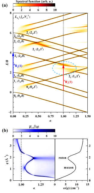
Figure 2: (a) Angulon spectral function for CH₃ as a function of the dimensionless energy $E/B$ and interaction parameter $\alpha$. The spectrum of Fig. 1(a) corresponds to $\alpha\equiv 1$ (dashed vertical line). The broadening of the $\mathrm{{}^{R}R_{1}(1)}$ line occurs due to the angulon instability (encircled). (b) Phonon density $|\beta_{311}(q)|^{2}$ in the vicinity of the angulon instability (left) and the experimentally measured dispersion relation of bulk ⁴He Donnelly and Barenghi (1998) (right). The phonon excitation takes place in the region of wavevectors $q\sim 2.5$ Å.

It is important to note that the qualitative discussion of Ref. Morrison, Raston, and Douberly (2013) attributed the broadening to excitation of at least two phonons, since the splitting between the $2_{2}$ and $1_{1}$ states ($\sim 21~{}\mathrm{cm^{-1}}$) exceeds the maximum energy of an elementary excitation in superfluid ⁴He ($\sim 14~{}\mathrm{cm^{-1}}$ Manousakis and Pahdharipande (1986)). The results presented above demonstrate that the broadening can be explained as a one-phonon transition between two many-particle states, $2_{2}(2_{2},0)$ and $2_{2}(1_{1},1^{3})$. In other words, in the presence of the superfluid, the level structure of the dressed molecule changes, and the energy conservation arguments have to be modified accordingly.

Thus, we have generalized the angulon theory to the case of light symmetric-top molecules and demonstrated that angulon instabilities predicted in Refs. Schmidt and Lemeshko (2015, 2016) have in fact been observed in the spectra of CH₃ and NH₃ immersed in superfluid helium nanodroplets. This paves the way to studying the decay of angulon quasiparticles and other microscopic mechanisms of the angular momentum transfer in experiments on quantum liquids, with possible applications to phonon quantum electrodynamics Soykal, Ruskov, and Tahan (2011). Furthermore, the angulon instabilities have been predicted to lead to anomalous screening of quantum impurities Yakaboylu and Lemeshko (2017) as well as to the emergence of non-abelian magnetic monopoles Yakaboylu, Lemeshko, and Deuchert , which opens the door for the study of exotic physical phenomena in helium droplet experiments. Future measurements on isotopologues, such as CD₃ or ND₃, would allow the variation of the molecular rotational constants without altering the molecule-helium interactions, thereby providing an additional test of the model. It would be of great interest to perform quench experiments involving short laser pulse excitations Pentlehner et al. (2013); Shepperson et al. (2017a, b) of CH₃ and NH₃ in helium nanodroplets aiming to observe the dynamical emergence of the angulon instability.

S1 Supplemental Material

S1.1 Derivation of the angulon hamiltonian

The Hamiltonian for a rotating molecule interacting with a bath of bosons has the following structure: $\hat{H}=\hat{H}_{\text{mol}}+\hat{H}_{\text{bos}}+\hat{H}_{\text{mol-bos}}$. The present derivation for a symmetric-top impurity is analogous to the linear impurity case described in detail in Refs. Lemeshko and Schmidt (2017); Schmidt and Lemeshko (2015, 2016). For a symmetric-top impurity, the anisotropic molecule-helium potential is expanded in spherical harmonics as follows Green (1976, 1980):

$$V_{\text{mol-He}}(r,\theta,\phi)=\sum_{\lambda\xi}V_{\lambda\xi}(r)(1+\delta_{\xi 0})^{-1}[Y_{\lambda\xi}(\theta,\phi)+Y_{\lambda\xi}^{*}(\theta,\phi)]$$ (S1)

Here $(r,\theta,\phi)$ describe the position of the helium atom with respect to the center of mass of the molecule in the molecular (body-fixed) coordinate system. Spherical components, $V_{\lambda\xi}(r)$, of the PES for the CH${}_{3}-$He and NH${}_{3}-$He complexes Dagdigian and Alexander (2011); Suarez et al. (2011) are shown in Fig. S1.

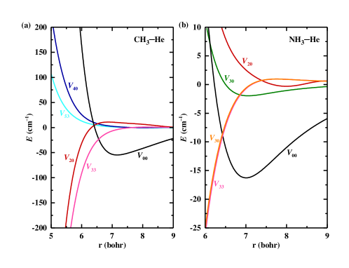
Figure S1: (a) Spherical components, $V_{\lambda\xi}(r)$, of the CH${}_{3}-$He PES Dagdigian and Alexander (2011). (b) Same as (a) for NH${}_{3}-$He Suarez et al. (2011).

The pairwise interaction potential determines the explicit form for the last term of the Hamiltonian (LABEL:eq:hamil), which contains the coupling constants $v_{\lambda\xi}(q)$, defined as:

$$v_{\lambda\xi}(q)=\sqrt{\frac{2nq^{2}\epsilon(q)}{\pi\omega(q)}}(1+\delta_{\xi 0})^{-1}\int drr^{2}f_{\lambda\xi}(r)j_{\lambda}(rq)$$ (S2)

Here $\epsilon(q)=\frac{q^{2}}{2m}$ is the kinetic energy of a boson of mass $m$, and $j_{\lambda}(rq)$ are spherical Bessel functions. We choose model interaction potentials characterized by the Gaussian form-factors, $f_{\lambda\xi}(r)=u_{\lambda\xi}(2\pi)^{-3/2}e^{-\frac{r^{2}}{2r_{\lambda\xi}^{2}}}$, with parameters $r_{\lambda\xi}$ corresponding to the global minimum of the CH₃–He (NH₃–He) PES. The isotropic component, $u_{00}$, was chosen such that it reproduces the mean-field shift (‘trapping potential’) of 40 $\mathrm{cm^{-1}}$, typical for small molecules in helium nanodroplets Toennies and Vilesov (2004). The mean-field shift can be expressed in terms of $f_{00}(r)$ as follows Lemeshko and Schmidt (2017):

$$E_{\text{mf}}=\sqrt{4\pi}n\int r^{2}f_{00}(r)dr$$ (S3)

The ratio of $u_{33}/u_{00}$ was fixed to satisfy the following condition:

$$\frac{\int^{\infty}_{0}drr^{2}f_{33}(r)j_{3}(rq)}{\int^{\infty}_{0}drr^{2}f_{00}(r)j_{0}(rq)}=\frac{\int_{r_{c}}^{\infty}drr^{2}V_{33}(r)j_{3}(rq)}{\int_{r_{c}}^{\infty}drr^{2}V_{00}(r)j_{0}(rq)},$$ (S4)

where $V_{\lambda\xi}(r)$ are the spherical components of the ab initio PES. The cut-off distance, $r_{c}$, was set to the classical turning point for a collision at the temperature inside a helium droplet, i.e. such that $V_{00}(r_{c})=k_{B}\times 0.4~{}\mathrm{K}$, with $k_{B}$ the Boltzmann constant Toennies and Vilesov (2004).

S1.2 The Dyson equation

Minimization of energy, $E=\langle\psi_{LMk_{0}}|\hat{H}|\psi_{LMk_{0}}\rangle/\langle\psi_{LMk_{0}}|\psi_{LMk_{0}}\rangle$, with respect to $Z^{1/2\ast}_{LMk_{0}}$ and $\beta_{\lambda jk}^{\ast}(q)$ leads to the Dyson-like equation Lemeshko and Schmidt (2017):

$$[G^{\text{ang}}_{Lk_{0}}(E)]^{-1}=[G^{0}_{Lk_{0}}(E)]^{-1}-\Sigma_{Lk_{0}}(E)=0,$$ (S5)

where

$$G^{0}_{Lk_{0}}(E)=\frac{1}{BL(L+1)+(C-B)k_{0}^{2}-E}$$ (S6)

is the Green’s function of the unperturbed molecule and $G^{\text{ang}}_{Lk_{0}}(E)$ is the angulon Green’s function. The energy can be found self-consistently, as a set of solutions to Eq. (S5) for a given total angular momentum $L$, which is the conserved quantity of the problem. Alternatively, one can reveal stable and meta-stable states of the system by calculating the spectral function Lifshitz and Pitaevskii (1980); Altland and Simons (2010); Lemeshko and Schmidt (2017):

$$\mathcal{A}_{Lk_{0}}=\mathrm{Im}[G^{\text{ang}}_{Lk_{0}}(E+i0^{+})]$$ (S7)

The spectral function (S7) corresponds to Eq. (5) with $\langle v^{\prime}|\langle\psi_{L^{\prime}M^{\prime}k_{0}^{\prime}}|\bm{\hat{\mu}}|\psi_{LMk_{0}}\rangle|v\rangle\equiv 1$.

S1.3 Matrix elements for spectroscopic transitions

Within the electric dipole approximation, the probability of a perpendicular optical transition between two angulon states, $|\psi_{LMk_{0}}\rangle|v\rangle$ and $|\psi_{L^{\prime}M^{\prime}k^{\prime}_{0}}\rangle|v^{\prime}\rangle$, is given by:

$$I_{LMk_{0},v}^{L^{\prime}M^{\prime}k^{\prime}_{0},v^{\prime}}\sim\frac{g^{\prime}}{g}|\langle v^{\prime}|\langle\psi_{L^{\prime}M^{\prime}k^{\prime}_{0}}|\bm{\mathrm{\hat{\mu}}}|\psi_{LMk_{0}}\rangle|v\rangle|^{2}$$ (S8)

where $g$ and $g^{\prime}$ give the degeneracies of the $|\psi_{LMk_{0}}\rangle|v\rangle$ and $|\psi_{L^{\prime}M^{\prime}k^{\prime}_{0}}\rangle|v^{\prime}\rangle$ states, respectively, $\bm{\mathrm{\hat{\mu}}}$ is the dipole moment operator. Substituting the angulon wavefunctions from Eq. (2), for a perpendicular optical transition, we obtain Bunker and Jensen (2006):

$$I_{LMk_{0},v}^{L^{\prime}M^{\prime}k^{\prime}_{0},v^{\prime}}\sim\frac{g^{\prime}}{g}|\langle v^{\prime}|\bm{\mathrm{\hat{\mu}}}|v\rangle|^{2}\left[Z^{1/2*}_{LMk_{0}}Z^{1/2}_{L^{\prime}M^{\prime}k^{\prime}_{0}}M_{LMk_{0}}^{L^{\prime}M^{\prime}k^{\prime}_{0}}+\sum_{\begin{subarray}{q}~{}q\lambda\mu\\ ~{}jmk\\ j^{\prime}m^{\prime}k^{\prime}\end{subarray}}\beta^{*}_{\lambda jk}(q)\beta_{\lambda j^{\prime}k^{\prime}}(q)C^{LM}_{jm,\lambda\mu}C^{L^{\prime}M^{\prime}}_{j^{\prime}m^{\prime},\lambda\mu}M^{j^{\prime}m^{\prime}k^{\prime}}_{jmk}\right]^{2}$$ (S9)

where $M^{jmk}_{j^{\prime}m^{\prime}k^{\prime}}$ is a rotational matrix element for the transition between the molecular states $|jmk\rangle$ and $|j^{\prime}m^{\prime}k^{\prime}\rangle$ Bunker and Jensen (2006).

$$M^{jmk}_{j^{\prime}m^{\prime}k^{\prime}}=\sqrt{\frac{2j+1}{8\pi^{2}}}\sqrt{\frac{2j^{\prime}+1}{8\pi^{2}}}\Bigg{[}\begin{pmatrix}1&j&j^{\prime}\\ 0&m&-m^{\prime}\end{pmatrix}\begin{pmatrix}-1&j&j^{\prime}\\ 0&k&-k^{\prime}\end{pmatrix}+\begin{pmatrix}1&j&j^{\prime}\\ 0&m&-m^{\prime}\end{pmatrix}\begin{pmatrix}1&j&j^{\prime}\\ 0&k&-k^{\prime}\end{pmatrix}\Bigg{]}$$ (S10)

S1.4 Corrections to the angulon energy

We corrected the energies of angulons states for the vibrational shift in He droplets, inversion splitting of NH₃ and Coriolis coupling. The shift of the vibrational frequency and ground-state inversion splitting of NH₃ were set to their empirical values: $\delta\nu=\nu_{\text{He}}-\nu_{\text{gas}}=0.08~{}\mathrm{cm^{-1}}$ for CH₃ Morrison, Raston, and Douberly (2013), $\delta\nu=-0.5~{}\mathrm{cm^{-1}}$, $\Delta^{\text{inv}}_{0}=0.8~{}\mathrm{cm^{-1}}$ for NH₃ Slipchenko and Vilesov (2005). The rotation-vibration Coriolis coupling is given by the following matrix element Bunker and Jensen (2006):

$$\langle v|\langle\psi_{Lk_{0}}|-2\zeta C\hat{\pi}^{\prime}_{z}\hat{J^{\prime}_{z}}|\psi_{Lk_{0}}\rangle|v\rangle=-2\zeta Cl\bigg{(}Z^{\ast}_{Lk_{0}}k_{0}+\sum_{qjk}|\beta_{\lambda jk}(q)|^{2}k\bigg{)}$$ (S11)

where $|\psi_{Lk_{0}}\rangle$ is the angulon state of Eq. (2), $\zeta$ is the constant parametrizing the Coriolis coupling, $\hat{\pi}^{\prime}_{z}$ is the vibrational angular momentum operator with respect to the symmetric top axis with eigenvalues $l$. For a given vibrational state $|v\rangle$, the vibrational angular momentum $|l|=v,v-2,\ldots,1$ or $0$. For the ground vibrational state $l=0$, and $|l|=1$ for the excited state under consideration, $|\nu_{3}=1\rangle$. We used the Coriolis constants $\zeta C=0.35$ cm^-1 for CH₃ Davis et al. (1997), and $\zeta C=0.29$ cm^-1 for NH₃ Guelachvili et al. (1989).

S1.5 Comparison to experiment

Table S1 lists the spectral characteristics of the experimental lines shown in Fig. 1(a), (b), as well as the results of the angulon theory. One can see that the angulon theory is able to reproduce the width of the ^RR₁(1) line, which is approximately one order of magnitude broader compared to other transitions. The model tends to underestimate the line broadening by a few GHz, which we attribute to the fact that only single-phonon excitations are included into the ansatz (2). Using more involved, diagrammatic approaches Bighin and Lemeshko (2017) to the Hamiltonian (LABEL:eq:hamil) is expected to further improve the agreement.

Table S1: Comparison of the $\nu_{3}$ spectral line frequencies, $\nu$ (in $\mathrm{cm^{-1}}$), and widths, $\Gamma$ (in GHz), obtained using the angulon model with the experimental ones. Spectral lines are labeled as ${}^{\Delta K}\Delta L_{K^{\prime\prime}}(L^{\prime\prime})$, where the initial state is marked with a double prime. We omit the $\bm{\mathrm{s}}$ and $\bm{\mathrm{a}}$ indices labelling the inversion splitting in NH₃ Ruzi and Anderson (2013).

Line	CH3				NH3
	Angulon theory		Experiment Morrison, Raston, and Douberly (2013)		Angulon theory		Experiment Slipchenko and Vilesov (2005)
	$\nu$	$\Gamma$	$\nu$	$\Gamma$	$\nu$	$\Gamma$	$\nu$	$\Gamma$
PP1(1)	3146.96	2.15	3147.0161(2)	4.12(1)	3427.29	6.46	3427.5	10(1)
PQ1(1)	3165.60	2.27	3165.6899(2)	3.77(2)	3445.63	6.52	3445.9	21(6)
RR0(0)	3173.97	2.36	3174.2373(1)	4.66(1)	3456.92	6.68	3457.3	11.1(3)
RR1(1)	3182.61	49.92	3182.410(6)	57.0(6)	3469.11	47.11	3468.8	50(10)
PR1(1)	3203.15	2.46	3203.080(1)	8.6(1)	–	–	–	–