Graphical Methods in Device-Independent
Quantum
Cryptography
Abstract
We introduce a framework for graphical security proofs in device-independent quantum cryptography using the methods of categorical quantum mechanics. We are optimistic that this approach will make some of the highly complex proofs in quantum cryptography more accessible, facilitate the discovery of new proofs, and enable automated proof verification. As an example of our framework, we reprove a previous result from device-independent quantum cryptography: any linear randomness expansion protocol can be converted into an unbounded randomness expansion protocol. We give a graphical proof of this result, and implement part of it in the Globular proof assistant.
1 Introduction
Graphical methods have long been used in the study of physics and computation. In physics, this can be traced back at least as far as Penrose’s use of diagrams [1]. During the last decade of the twentieth century, rigorous methods for graphical reasoning in monoidal categories were developed by Joyal, Street, and others [2, 3]. When Abramsky and Coecke proposed monoidal categories as an alternative foundation for quantum physics [4], they were able to draw from these technical developments to introduce an elaborate graphical language for reasoning about quantum mechanical concepts. Since then, the use of rigorous graphical methods has been extended widely, ranging from foundations [4] to quantum algorithms [5], quantum error correction [6], and beyond [7, 8]. The great success of graphical methods in the quantum sciences is largely due to their ability to deal with elaborate concepts in a simple way. This is especially true when compared to the standard methods involving linear operators acting on Hilbert space.
Quantum cryptography, the study of cryptographic protocols that are based on quantum mechanical principles (see Section 12.6 of [9] for an introduction) is an ideal candidate for graphical analysis. Indeed, proofs in quantum cryptography are often long and complicated even when the central idea of the proof is relatively clear. Pictures are regularly used as a conceptual aid in discussions of quantum cryptography, but it would be beneficial for both accessibility and rigor if proofs themselves could be expressed as pictures. For this reason, we believe that the field of quantum cryptography can benefit from the abstract methods of categorical quantum mechanics [8].
To our knowledge the use of graphical methods to formalize quantum cryptography is fairly new, although the literature provides some useful beginnings. Graphical security proofs for quantum key distribution (one of the original problems in the field) have been presented in [10, 11, 12], although these are not yet at the level of security that has been proved through non-graphical means. Meanwhile, the literature has a number of formal treatments of cryptography that are not primarily based on graphical reasoning. An important example is [13], which has a focus similar to the current paper. See also [14, 15, 16, 17].
One of the recent major achievements of quantum cryptography is the development of device-independent security proofs [18]. In such proofs, not only the adversary but also the quantum devices are untrusted, and allowed to exhibit uncharacterized behavior. Protocols in this field always include a classical test of the quantum devices which lead to a “succeed” or “abort” event at the end of the protocol, and we must prove that if the protocol “succeeds,” then the desired cryptographic task has been securely carried out. Device-independence is a desirable level of security for quantum cryptography (in particular because it accounts for arbitrary noise or imperfection in the quantum hardware) and it will be our focus in this paper.
As a specific problem to study, we consider device-independent randomness expansion. Research over the last decade has led to a proof that random numbers can be generated with devices that are completely untrusted [19, 20, 21, 22, 23, 24, 25, 26, 27, 28, 29, 30, 13]. Precisely, two untrusted quantum devices, together with a perfectly random seed of length , can be manipulated by a classical user to generate a perfectly random output of size with negligible error. See [31] for a gentle introduction to this topic and [32] for a discussion of a possible implementation.
Going further, it has been proved that one can take two copies of such a randomness expansion protocol (using different pairs of devices for each copy) and cross-feed them to produce an arbitrarily large quantity of random bits from a fixed-length seed [23, 13, 28]. Proving that randomness expansion can be extended in this way is not easy (indeed, the paper containing the first proof of unbounded expansion [33] was 34 pages long). Here, we give a proof of this extension (based on [13, 28]) using a graphical language. Explicitly, we prove that any secure protocol for linear randomness expansion implies a secure protocol for unbounded randomness expansion. The proof is based on formal graphical reasoning and is fairly compact.
A great benefit of graphical proofs is they are amenable to computer verification. The Globular proof assistant software [34] carries out category-theoretic proofs, using diagrams that are easily compatible with graphical languages for quantum mechanics. To further demonstrate the utility of our work we implemented the proof of unbounded randomness expansion in Globular. The proof is available as a video at [35].
This paper is organized as follows. In Section 2 we formalize a language to deal with quantum processes, building on the diagrammatic language given [36, 37]. Section 3 provides the formal basis for quantum cryptographic protocols that are based on untrusted devices. In Section 4 we give the proof that linear randomness expansion implies unbounded randomness expansion, and comment on our use of computer-assisted proof software. We conclude and discuss future work in Section 5.
The recent paper [38] also addresses graphical proofs of quantum cryptography, albeit with a different focus (device-dependent quantum key distribution). The graphical concepts in the present paper and in [38] were developed independently, and we expect that there will be a useful synergy between the two papers.
1.1 Our contributions
The graphical language used in this paper is based primarily on [36, 37]. We added new elements to enable quantum cryptographic proofs. Here are some of the additions:
-
1.
Diagrams for sets of processes. Whereas a diagram in the language of [36, 37] represents a quantum process, we expanded this to allow diagrams with uncharacterized elements to represent sets of processes. This is especially useful in the device-independent context for expressing security statements (see Definition 2.2).
-
2.
Approximations. We use the symbol when the state represented by one diagram is approximately equal to the state represented by another. This allows proofs via chains of approximations. A similar feature was independently used in [38].
-
3.
Duplication of states. We define the “duplication” of a classical-quantum state (see Section 2.3), a convenient shorthand which subsumes both the copying of classical states and the purification of quantum states.
-
4.
A graphical formalization of device-independence. We give a graphical formalization of what it means for a protocol to be device-independent (Section 3.2).
2 Fundamentals
In this section, we cover useful graphical techniques and concepts, building on [36, 37]. First, we describe the graphical language of categorical quantum mechanics. Next, we introduce a notion of distance between diagrams. Finally, we define the process of duplicating states. For further details the reader is encouraged to consult [36, 37] or the more recent [8] for categorical quantum mechanics, and [39] for notions of distance relevant to quantum information theory.
2.1 The graphical language of categorical quantum mechanics
Throughout, denotes a collection of finite-dimensional Hilbert spaces, each with a fixed orthonormal basis. We use Dirac notation when it is convenient: for any , we denote the fixed orthonormal basis by (with the subscript typically dropped). For any , the expression is simply another way of writing the vector , and denotes the dual of .
We assume that is closed under tensor products (i.e., if then ) and contains the space for every non-negative integer . We sometimes refer to the elements of as types or registers. The elements of are the objects of the category in which our graphical reasoning takes place. We refer the reader to [8] for further details. To simplify the notation in our diagrams, we sometimes write to represent the -bit quantum register .
We say that is a process of type if is a linear operator whose domain is and whose codomain is . It is represented by a box labeled whose input and output wires are labeled with the types and as follows.
|
|
(1) |
Note that diagrams are read from bottom to top. The identity operator is a process represented by a box-less diagram (below, left). The composition and tensor product of processes are respectively represented by the vertical and horizontal composition of diagrams (below, center and right).
|
|
(2) |
Note that two processes can be vertically composed only if their types are compatible. A process with no input wires is a state. A state of type should be interpreted as a vector in and is represented by the first diagram on the left below. The conjugate, transpose, and conjugate-transpose (i.e., adjoint) of are also depicted below (second, third, and fourth diagram respectively).
|
|
(3) |
A process with no output wires is called an effect. A process with no input and no output is a number, and is represented by a diamond whose label indicates its value.
Let be a register. Then the diagram
|
|
(4) |
denotes the vector and is called a spider. Spiders can have an arbitrary number of outgoing wires (with all of the wires being of the same type, and the definition extending in the obvious way). Because they will play an important role below, we will also introduce the uniform vector, which is denoted by a gray node:
| (5) |
where . The diagram on the left-hand side of (5) denotes the vector .
A quantum type, or quantum register, is an element of of the form . To graphically distinguish them for their classical counterparts, quantum states, effects, and processes are drawn with thick lines as in the diagrams below.
|
|
(6) |
A pure quantum state is a state of the form with . Graphically, a quantum state is pure if it satisfies the diagrammatic equality below.
| (7) |
A mixed quantum state of is a state of the form satisfying . A subnormalized mixed state is only required to satisfy . Unless otherwise specified, the word “state” refers to a normalized mixed state.
The above definition can be related to more conventional notation for quantum states (see, e.g., [39]) as follows. If
| (8) |
is a density operator on the vector space which represents a quantum state in the conventional sense, then the corresponding quantum state in the notation that we are using is given by
| (9) |
The main difference between (8) and (9) is that (8) is a linear map from to , while (9) is simply an element of .
A linear map is a quantum effect if it maps all states to the interval . In other words, is a quantum effect if
| (10) |
for all quantum states of . Effects correspond to positive semidefinite operators on with operator norm less than or equal to one. The effect given by is denoted by the diagram below
|
|
(11) |
and corresponds to taking the trace of a linear operator. If is a classical register then
|
|
(12) |
denotes the linear map given by .
For use in later proofs, we note the obvious fact that uniform states absorb terminations, i.e.,
| (13) |
A causal quantum process from a register to a register is a linear homomorphism such that for any state of , the diagram below represents a state.
|
|
(14) |
A stochastic quantum process is one that satisfies the same condition, with the weaker requirement that the diagram above is a subnormalized quantum state. Intuitively, a causal process is a process that always gives an outcome, while a stochastic process is a process that may sometimes “fail” and give no outcome (hence the trace of its output state may be smaller than the trace of its input state). Unless otherwise specified, the phrase “quantum process” refers to a stochastic quantum process.
Diagrammatically, a process is causal if and only if the process of applying and then discarding its output wires is equal to the process of merely discarding the input wires, e.g.,
| (15) |
Causal quantum processes correspond to completely positive trace-preserving maps in the conventional notation.
A pure process is a quantum process of the form
| (16) |
Note that pure processes map pure subnormalized states to pure subnormalized states.
If is a state of , then we can terminate one of its wires and obtain a state of :
|
|
(17) |
(This corresponds to taking a partial trace in the conventional framework.)
If is a register, then a classical state is a vector of the form , where is a probability distribution. If is a quantum register, then a classical-quantum state of is a state of the form , where is a probability distribution and each is a normalized state of . A quantum process on that is controlled by the classical register is a process of the form , where each is a process on .
In our context, it will be useful to represent sets of linear maps diagrammatically. A diagram in which every element is specified by an explicit linear map can itself be regarded a linear map (obtained by composition and tensor product). A diagram in which some elements are unspecified represents the set of all specifications of that form. For example, the following diagrams
|
|
(18) |
represent, respectively, the set of all (normalized, mixed) states on , the set of all stochastic quantum processes , and the set of all classical-quantum states in which the classical register is and the quantum register can be arbitrary. Notice that when a wire is unlabeled and otherwise unspecified, the quantification ranges over all (quantum or classical) registers. Similarly, the diagram represents an arbitrary element of the interval .
2.2 Approximations
In what follows, we will need to be able to discuss the distance between certain processes. We therefore define a relation between diagrams which captures the appropriate metric (half of the diamond norm distance — see [39] for further details).
Definition 2.1.
If , , and are real numbers, we write if . Let and be two processes of the same type. Then, we write if for all states and effects ,
| (19) |
Note that the above definition remains equivalent if the phrase “for all states ” is replaced by “for all pure states .”
It follows from the definition that the notion of approximation defined above satisfies the triangle inequality (if and , then ) and that it is preserved by composition (if , then and for all stochastic processes of appropriate input and output type). If we restrict the processes and to be states (i.e., to have no inputs) then if and only if and differ by no more than in trace distance.
We now generalize the notion of distance between processes to a notion of distance between sets of processes. A similar notion of approximation appears in the non-graphical formalism of [15].
Definition 2.2.
Let and be two sets of processes, all of which have the same type. We write if for every , there exists such that . Moreover, we write if and .
These relations also satisfy a triangle inequality: if and , then . Note that the symbol is used to denote a relation between numbers, a relation between processes, and a relation between sets of processes. However, it will always be clear from the context whether numbers, processes, or sets of processes are being compared so that no ambiguity should arise from this slight abuse of notation.
2.3 Duplication
We now introduce the notion of duplicate states. Informally speaking, duplicating a classical-quantum state means copying its classical component and purifying its quantum component. See section 2.5 of [9] for a discussion of the notion of quantum state purification.
If is a subnormalized classical-quantum state of a register , then we can write , where . The matrices are then positive semidefinite. We can alternatively express as
| (20) |
where is the linear map defined by
| (21) |
Then, the canonical duplicate state of is given by
| (22) |
See equation (59) in the appendix for an expression for this state in conventional notation. Note that
| (23) |
More generally, a state of is a duplicate state (or simply duplication) of if (23) holds (with replaced by ) and has the form , where each is a pure subnormalized state of . Note that if is a classical state (with no quantum component), then there is only one duplicate of , and that is the “copied” state .
Duplicate states have the following universality property: for any subnormalized classical-quantum state of , where is a quantum register and is a classical register, such that
| (24) |
there exists a causal process from to satisfying
| (25) |
Additionally, if and are any two states of that are both duplicate states of , then there exists a unitary operator on , controlled by the register , such that
| (26) |
The following proposition follows from standard techniques and is proved in Appendix A.
Proposition 2.3.
If are subnormalized states that satisfy , and denote their respective canonical duplicate states, then .
The next corollary will be useful in later proofs.
Corollary 2.4.
Suppose that
| (27) |
and let be a state on that is a duplicate of . Then, there exists a causal process from to satisfying
| (28) |
Proof.
Let denote the canonical duplicate state of . By the property noted in equation (26) above, it suffices to prove the desired relation (28) with replaced by . By Proposition 2.3, the canonical duplicate state of the state on the left side of (27) satisfies . There is a causal process from to such that
| (29) |
Applying the same process to yields a state that is within distance from . ∎
3 Untrusted quantum processes
An untrusted quantum process is represented by a diagram in which all of the quantum processes are unlabeled and all of the classical processes are labeled. We discuss an example of such processes and then give a definition of the more specific class of device-independent quantum protocols.
3.1 Example: Quantum strategies for nonlocal games
A nonlocal game is a game played by parties () in which the players are given random inputs according to some fixed joint probability distribution. The players produce outputs and these outputs are scored as , where is a deterministic function that maps to . An example (the Clauser-Horne-Shimony-Holt game) is given below. The registers are classical bit registers (each isomorphic to ).
|
|
(30) |
The effect at the top denotes the map given by . This game is a common building block for device-independent protocols (including in particular the randomness expansion results that we will consider in section 4).
3.2 Device-independent quantum protocols
We are now ready to formalize the notion of a protocol in the device-independent setting. Historically, a quantum protocol is device-independent if all of its quantum processes are untrusted and uncharacterized (whereas strictly “classical” aspects, such as timing, non-communication, and computation, are still trusted). This definition can be traced back to early papers such as Mayers and Yao [18] and Ekert [40]. There is some room for interpretation as to exactly which quantum processes are allowed in device-independence, and we offer a specific formalism here. (Our treatment can be compared to the non-graphical formalization of device-independent protocols in section 4 of [13].)
For simplicity our definition is for a -device protocol, but it could easily be generalized to an -device protocol.
Definition 3.1.
A device-independent protocol with quantum devices is a diagram of the form
|
|
(31) |
where is constructed from the following subdiagrams.
-
1.
Communication between devices. An untrusted process transferring information (one way) from one of the two quantum registers to the other:
(32) -
2.
Deterministic classical functions. A deterministic function is applied to the register .
(33) -
3.
Failure. The value of the classical register is checked to see if it lies in a chosen subset ; if it does not, the protocol aborts. (Diagrammatically, this is the linear map from to given by .)
-
4.
Giving input to a device. A deterministic function is applied to and the result is given to one of the devices.
(34) -
5.
Receiving input from a device. Classical information is received from one of the devices.
(35)
Note that every device-independent protocol has two representations: as a diagram (including some unlabeled elements) and as a set of processes from to . We may use the label to refer to either representation. Device-independent protocols can be composed (e.g., the output quantum states of one protocol can be given as inputs to another, which corresponds to re-using the devices from the first protocol in the second).
4 Randomness expansion
4.1 Linear randomness expansion
We can now phrase security results on device-independent randomness expansion [22] in terms of diagrams. A device-independent randomness expansion protocol accepts a seed and returns a larger output. Security results for such protocols consist of asserting that if the seed is uniformly random, then except with negligible probability, the output is also uniformly random. The protocols that we consider for randomness expansion consist of iterating untrusted devices many times, and sometimes at random playing a nonlocal game (such as the CHSH game) to test that the devices are behaving properly (see Figure 2 in [28]).
A simple way to assert security for a -device randomness expansion protocol is to say that replacing the output with a true uniformly random state has a negligible effect, i.e.,
| (36) |
Above we compressed the two device states of into a single thick wire, and we are using the labels and as a shorthand for and . But it is preferable to have a stronger assertion: we wish to know that the output of the protocol is also approximately uniform when conditioned on the seed and on any quantum information entangled with the devices. The following theorem captures this stronger assertion.
Theorem 4.1 (Spot-check protocol).
There exist device-independent protocols , where has classical input dimension and classical output dimension , and there exists a function , such that the following hold.
-
1.
Soundness. For any and any state ,
(37) -
2.
Completeness.
(38)
“Soundness” asserts that the protocols must either produce random numbers or fail. “Completeness” asserts that there exist processes which will make succeed with probability approaching .
The following corollary will be a key step in our proof of unbounded randomness expansion. Whereas Theorem 4.1 assumes that the state of the devices is destroyed, the next lemma addresses the case where the device-state is preserved. In any diagram, let denote the set of all causal processes (with input and output types as implied by the diagram).
Lemma 4.2 (Spot-Check Lemma).
There exists such that for every integer ,
| (39) |
Proof.
Let be as in Theorem 4.1, let be a positive integer, and let . We have
| (40) |
for any pure state . We construct a duplication of the state on the right side of the above equation. Let denote the quantum register represented by the thick input wire received by the process . The effect
| (41) |
is an element in the dual of which can be written as , where the matrices are positive semidefinite. Let denote the controlled pure process
| (42) |
Then, the state
|
|
(43) |
is a duplication of the state
|
|
(44) |
Likewise, the state
|
|
(45) |
is a duplication of the state on the right side of (40). Therefore by Corollary 2.4, there is a causal process such that
| (46) |
The desired result follows (with ). ∎
Additionally, we note the following alternative form of the completeness assertion for . The next lemma asserts that the set of all possible classical outputs of the spot-checking protocol must contain a state that is close to the (normalized) uniform state on . This is similar to the use of “adjustment completeness error” in [28].
Lemma 4.3.
There exists such that
| (47) |
Proof.
Combining the soundness and completeness claims in Theorem 4.1, we have
| (48) |
The desired result follows, with . ∎
4.2 Unbounded randomness expansion
Now we discuss a graphical proof of unbounded (rather than linear) randomness expansion. We would like to apply the spot-checking protocol and lemma repeatedly, in order to obtain unbounded randomness expansion. Naively stacking operations atop one another does not work. Intuitively, this is because the results of subsection 4.1 only apply if the initial seed is independent of the state of the devices in the protocol . If we reuse devices in two successive iterations of the protocol, that independence assumption may not hold. However, it was observed in [13, 23, 28] that we can still obtain unbounded randomness by employing two pairs of devices and alternating which pair is employed in the protocol. In effect, one proves that the second application of the protocol wipes out any correlation with the first device, which may then be used in the third step to erase correlation with the second, and so on.
Definition 4.4.
For any integer , let denote the set of processes given by
|
|
where denotes the process set from Theorem 4.1. Let denote the composition .
We prove the following lemma (which will be a building block for a later induction proof). For the remainder of this section, let be the error function from Lemma 4.2.
Lemma 4.5.
For every integer , we have
| (49) |
where .
Proof.
We first use Definition 4.4 to expand the left-hand side of Equation 49 and then apply Lemma 4.2 to the occurrence of in the resulting diagram.
| (50) |
We can now move the spider of type along its wire to place it below the occurrence of and apply Lemma 4.2 again.
| (51) |
In the rightmost diagram above, the three lower boxes form a stochastic process, and this completes the proof. ∎
Lemma 4.6.
For all integers , we have
| (52) |
where .
Proof.
By induction on . The case follows from Lemma 4.5 by setting . So suppose that . Then we can expand the left-hand side of Equation 52 and apply the induction hypothesis to obtain
| (53) |
where and . The desired result follows. ∎
Theorem 4.7 (Soundness for Unbounded Expansion).
There is a function such that for any ,
| (54) |
Proof.
By the property noted in Equation 13, we can add a terminated branch to the left-hand side of Equation 54 so that we can apply Lemma 4.6.
| (55) |
We next apply causality (see the discussion of Equation 15) followed by Equation 13.
| (56) |
The set of processes described by the rightmost diagram consist of a uniform state of dimension together with a subnormalized state of , as desired.
Let , which upper bounds the error term . Note that for any nonnegative function on the set
| (57) |
Thus . This completes the proof. ∎
4.3 Formalization
In addition to their intuitive appeal, the graphical structures of categorical quantum mechanics are amenable to computer formalization. In the long term, this will be critically important for managing the complexity of medium- and large-scale security proofs. In this respect, computers can play a number of roles including validation and verification, copying and reuse, and proof search and discovery.
As part of our investigations, we have produced a computer-verified skeleton version of the main sequence of steps from our proof, for the case . We used the Globular proof assistant [34]. The reader can find and explore the proof object at [42], and a video of the diagrammatic moves involved in the proof is available at [35]. The Globular proof assistant provides a system for creating string diagram proofs, based on the perspective of higher-dimensional re-writing. In this project we used the system to prototype our arguments, and found the tool quite useful despite a few rough edges.
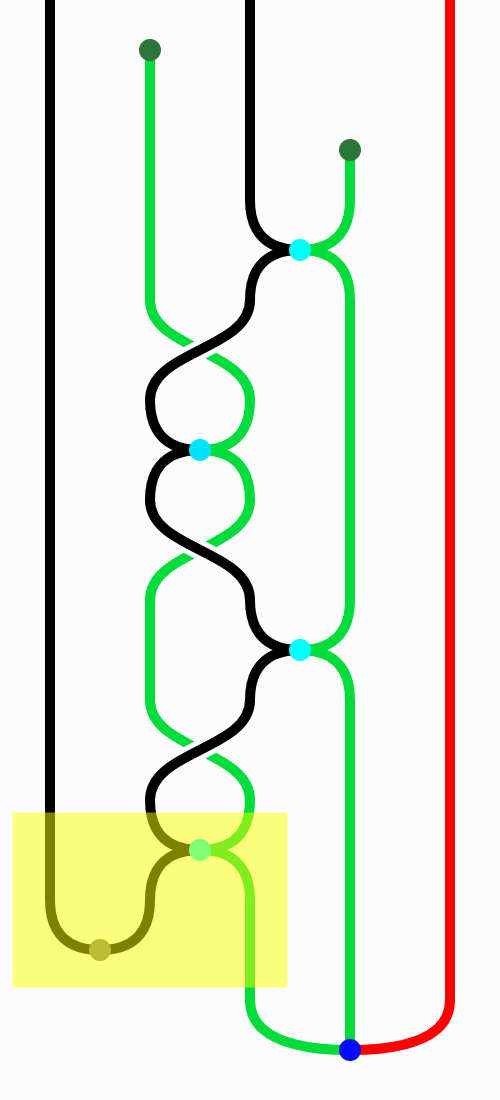
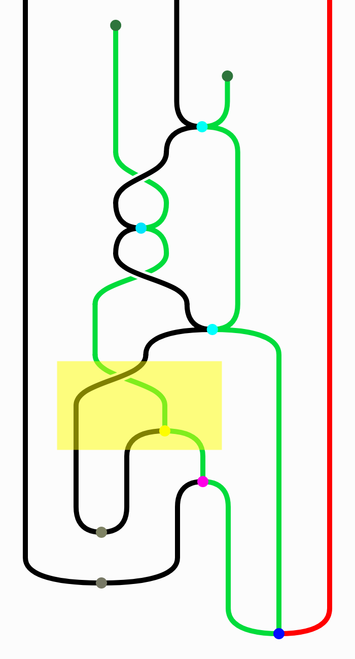
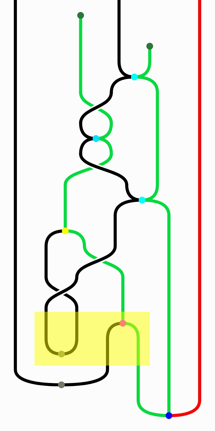
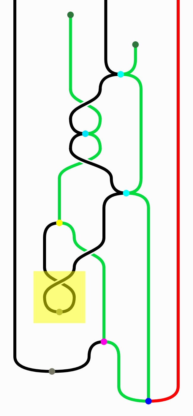
In Globular, one begins by declaring generators, atomic components which can be joined together into more complex diagrams. These generators come in several dimensions; strings in dimension 1 (classical, quantum), processes in dimension 2 (e.g., the spot-check protocols), and equations in dimension 3 (e.g., the spot-check lemma, the causality principle). More general protocols are complex two-dimensional diagrams. A proof becomes a three-dimensional diagram, though we often think of it as a “movie” whose frames are iterated slices of the 3-D diagram, tracing through the diagrammatic moves of the proof.
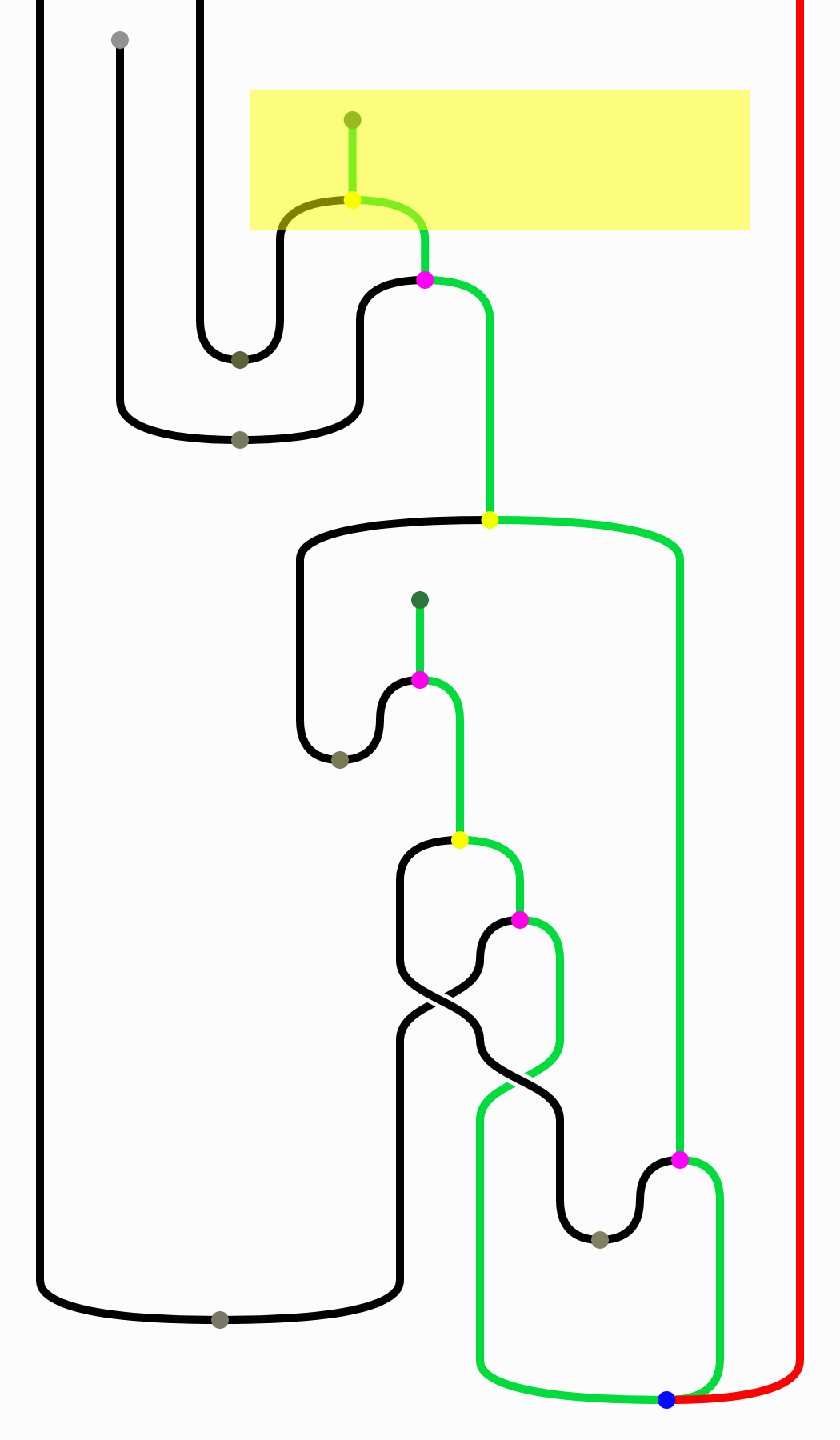
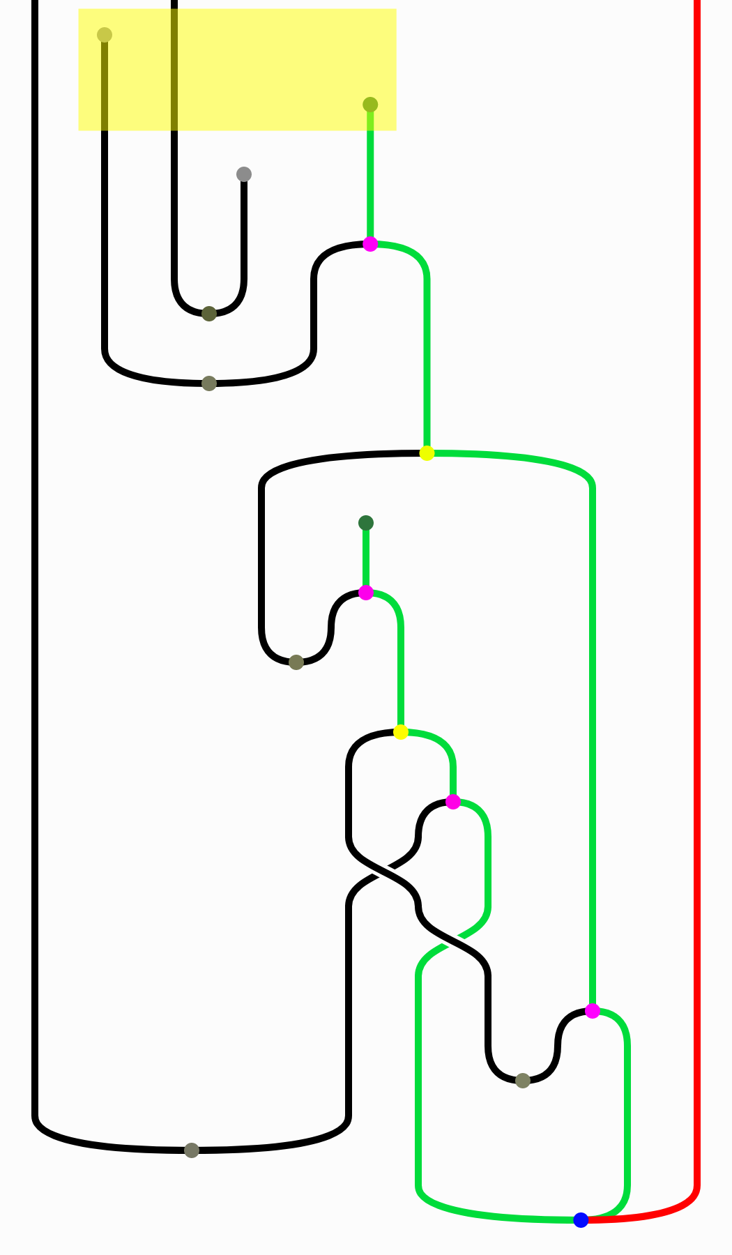
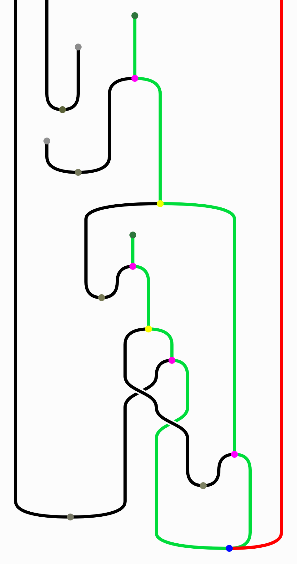
We used Globular to prototype the proof of Theorem 4.7. In particular, we used it to prototype and validate the general strategy of our proof in the case . Figure 1 shows part of the sequence of Globular diagrams in our proof of Theorem 4.7 for ; the entire sequence involved 60 steps. (The sequence includes four applications of Lemma 4.2 followed by the final application of causality.)
 |
 |
 |
 |
… |  |
 |
… |  |
| 0 | 1 | 2 | 3 | … | 55 | 56 | … | 60 |
We found several significant benefits to building proofs in Globular. As diagrams become more complex, our ability to manipulate them with pen and paper is limited. Globular automates the management of diagrams, allowing for easy reuse and undo.
The proof assistant also “type-checks” the user, admitting only valid constructions and proof. This allows the user to explore the space of possible diagrams and proofs without accidentally introducing errors. This will be particularly important for learning because it permits a focus on concepts over calculation.
More generally, formalization serves to identify gaps in our reasoning. In this case, we first identified the graphical form of the spot-check lemma (Lemma 4.2) and the final form of Theorem 4.7. By trying to prove the theorem in Globular we first validated the back-and-forth approach described in the proof of our theorem, but also showed that it was insufficient to yield our desired result. This, in turn, helped to identify the role of causality in our argument.
Overall, we found the Globular proof assistant to be quite helpful in prototyping and managing our arguments, although some issues limit its practical application. For example, three steps are needed to pass from step 56 to step 60 (see above), despite the fact that the two diagrams are more-or-less identical. This problem reifies as diagrams become more complicated; in our proof, 19 steps of sliding operations were needed between the second and third applications of the spot-check protocol. Improvements to such tools, both in underlying computation and representation and in user interface would be valuable areas for future research.
5 Conclusion
Our graphical proof of unbounded expansion was based on two central steps: one was the application of the Spot-Check Lemma (Lemma 4.2), and the other was the principle of causality. Causality is an elementary step in symbolic proofs for quantum information, but in the case of our graphical proof it is an important manipulation.
We have used the tools of categorical quantum mechanics to give a streamlined proof that unbounded randomness expansion can be obtained via the spot-checking protocol. We hope to have convinced the reader of the usefulness and potential of graphical methods in quantum cryptography for proof exposition. Also, when graphical proofs are appropriately created, they open the door to automated proof-checking. Our experience using the Globular proof assistant can be seen as interesting case study in the usefulness of the software and we hope that our experience can motivate future work.
Our goal for later work is to develop a language for quantum cryptography that allows a wide range of expositions of old results and proofs of new results. Some proofs (including unbounded randomness expansion) seem easiest to understand in graphical form, while others (such as Proposition 2.3) may be most accessible as algebraic proofs. Thus, an ideal framework would allow easy translation back and forth between algebraic and graphical expositions.
Acknowledgements
We are greatly indebted to David Spivak for providing some of the original inspiration for this project and for helping us to get it started. CAM would also like to thank Brad Lackey for seminars at the University of Maryland that deepened his understanding of axiomatic quantum information. NJR is funded by the Department of Defense. This paper includes contributions from the U. S. National Institute of Standards and Technology, and is not subject to copyright in the United States.
References
- Penrose [1971] R. Penrose, in Combinatorial Mathematics and its Applications, edited by D. Welsh (Academic Press, New York, 1971) pp. 221–244.
- Joyal and Street [1991] A. Joyal and R. Street, Advances in Mathematics 88, 55 (1991).
- Selinger [2011] P. Selinger, “A Survey of Graphical Languages for Monoidal Categories,” in New Structures for Physics (Springer Berlin Heidelberg, Berlin, Heidelberg, 2011) pp. 289–355.
- Abramsky and Coecke [2004] S. Abramsky and B. Coecke, in Proceedings of the 19th Annual IEEE Symposium on Logic in Computer Science (LICS 2004) (2004) pp. 415–425.
- Vicary [2013] J. Vicary, in Proceedings of the 28th Annual ACM/IEEE Symposium on Logic in Computer Science (LICS 2013) (2013) pp. 93–102.
- Chancellor et al. [2016] N. Chancellor, A. Kissinger, S. Zohren, and D. Horsman, “Coherent Parity Check Construction for Quantum Error Correction,” (2016), available from arXiv:1611.08012.
- Coecke [2016] B. Coecke, “From Quantum Foundations via Natural Language Meaning to a Theory of Everything,” (2016), available from arXiv:1602.07618.
- Coecke and Kissinger [2017] B. Coecke and A. Kissinger, Picturing Quantum Processes: A First Course in Quantum Theory and Diagrammatic Reasoning (Cambridge University Press, 2017).
- Nielsen and Chuang [2002] M. A. Nielsen and I. L. Chuang, Quantum Computation and Quantum Information (Cambridge University Press, 2002).
- Coecke and Perdrix [2010] B. Coecke and S. Perdrix, in Computer Science Logic: 24th International Workshop, CSL 2010, 19th Annual Conference of the EACSL, Brno, Czech Republic, August 23-27, 2010. Proceedings (Springer Berlin Heidelberg, Berlin, Heidelberg, 2010) pp. 230–244, preprint available from arXiv:1004.1598.
- Coecke et al. [2011] B. Coecke, Q. Wang, B. Wang, Y. Wang, and Q. Zhang, in Proceedings of the 6th International Workshop on Quantum Physics and Logic (QPL 2009) (2011) pp. 231 – 249.
- Hillebrand [2012] A. Hillebrand, in Proceedings of the 8th International Workshop on Quantum Physics and Logic (QPL 2011) (2012) pp. 103–121.
- Chung et al. [2014] K.-M. Chung, Y. Shi, and X. Wu, “Physical Randomness Extractors: Generating Random Numbers with Minimal Assumptions,” (2014), available from arXiv:1402.4797.
- Heunen [2008] C. Heunen, Logical Methods in Computer Science 4, 4 (2008).
- Maurer and Renner [2011] U. Maurer and R. Renner, in Innovations in Computer Science (Tsinghua University Press, 2011) pp. 1–21.
- Pavlovic [2014] D. Pavlovic, in Categories and Types in Logic, Language, and Physics - Essays Dedicated to Jim Lambek on the Occasion of His 90th Birthday, Vol. 8222 (2014).
- Stay and Vicary [2013] M. Stay and J. Vicary, Electronic Notes in Theoretical Computer Science 298, 367 (2013), proceedings of the Twenty-ninth Conference on the Mathematical Foundations of Programming Semantics, MFPS XXIX.
- Mayers and Yao [1998] D. Mayers and A. Yao, in Proceedings 39th Annual Symposium on Foundations of Computer Science (Cat. No.98CB36280) (1998) pp. 503–509.
- Arnon-Friedman et al. [2018] R. Arnon-Friedman, F. Dupuis, O. Fawzi, R. Renner, and T. Vidick, Nature Communications 9, 459 (2018).
- Arnon-Friedman et al. [2016] R. Arnon-Friedman, R. Renner, and T. Vidick, “Simple and Tight Device-Independent Security Proofs,” (2016), available from arXiv:1607.01797.
- Bierhorst et al. [2017] P. Bierhorst, E. Knill, S. Glancy, A. Mink, S. Jordan, A. Rommal, Y.-K. Liu, B. Christensen, S. W. Nam, and L. K. Shalm, “Experimentally Generated Random Numbers Certified by the Impossibility of Superluminal Signaling,” (2017), available from arXiv:1702.05178.
- Colbeck [2007] R. Colbeck, “Quantum And Relativistic Protocols For Secure Multi-Party Computation,” Ph.D. thesis, University of York (2007), available from arXiv:0911.3814.
- Coudron and Yuen [2014] M. Coudron and H. Yuen, in Proceedings of the Forty-sixth Annual ACM Symposium on Theory of Computing, STOC ’14 (ACM, New York, NY, USA, 2014) pp. 427–436.
- Dupuis et al. [2016] F. Dupuis, O. Fawzi, and R. Renner, “Entropy Accumulation,” (2016), available from arXiv:1607.01796.
- Fehr et al. [2011] S. Fehr, R. Gelles, and C. Schaffner, Physical Review A 87 (2011), 10.1103/PhysRevA.87.012335.
- Knill et al. [2018] E. Knill, Y. Zhang, and H. Fu, “Quantum probability estimation for randomness with quantum side information,” (2018), arXiv:1806.04553.
- Miller and Shi [2017] C. A. Miller and Y. Shi, SIAM Journal on Computing 46, 1304 (2017).
- Miller and Shi [2016] C. A. Miller and Y. Shi, Journal of the ACM 63, 33:1 (2016).
- Pironio et al. [2010] S. Pironio, A. Acín, S. Massar, A. Boyer de la Giroday, D. Matsukevich, P. Maunz, S. Olmschenk, D. Hayes, L. Luo, T. A Manning, and C. Monroe, Nature 464, 1021 (2010).
- Pironio and Massar [2011] S. Pironio and S. Massar, Physical Review A 87 (2011), 10.1103/PhysRevA.87.012336.
- Aaronson [2014] S. Aaronson, American Scientist 102, 266 (2014).
- National Institute of Standards and Technology () [NIST] National Institute of Standards and Technology (NIST), “Randomness Beacon Program,” https://www.nist.gov/programs-projects/nist-randomness-beacon, accessed: 2019-02-01.
- Coudron and Yuen [2013] M. Coudron and H. Yuen, “Infinite Randomness Expansion and Amplification with a Constant Number of Devices,” (2013), preprint available from arXiv:1310.6755.
- Bar et al. [2018] K. Bar, A. Kissinger, and J. Vicary, Logical Methods in Computer Science 14 (2018).
- Globular [2019a] Globular, “Video,” Available as ancillary material at arXiv:1705.09213 (2019a), accessed: 2019-04-25.
- Coecke and Kissinger [2015] B. Coecke and A. Kissinger, “Categorical Quantum Mechanics I: Causal Quantum Processes,” (2015), available from arXiv:1510.05468.
- Coecke and Kissinger [2016] B. Coecke and A. Kissinger, “Categorical Quantum Mechanics II: Classical-Quantum Interaction,” (2016), available from arXiv:1605.08617.
- Kissinger et al. [2017] A. Kissinger, S. Tull, and B. Westerbaan, “Picture-perfect Quantum Key Distribution,” (2017), available from arXiv:1704.08668.
- Watrous [2018] J. Watrous, The Theory of Quantum Information (Cambridge University Press, 2018).
- Ekert [1991] A. K. Ekert, Phys. Rev. Lett. 67, 661 (1991).
- Vazirani and Vidick [2012] U. Vazirani and T. Vidick, in Proceedings of the Forty-fourth Annual ACM Symposium on Theory of Computing, STOC ’12 (ACM, New York, NY, USA, 2012) pp. 61–76.
- Globular [2019b] Globular, “Proof,” http://globular.science/1904.001 (2019b), accessed: 2019-04-25.
- De et al. [2012] A. De, C. Portmann, T. Vidick, and R. Renner, SIAM Journal on Computing 41, 915 (2012).
- Bonchi et al. [2014] F. Bonchi, P. Soboci’nski, and F. Zanasi, in CONCUR 2014 - Concurrency Theory, Lecture Notes in Computer Science, Vol. 8704 (2014) pp. 435–450.
- Kissinger and Uijlen [2017] A. Kissinger and S. Uijlen, in Proceedings of the 32nd Annual ACM/IEEE Symposium on Logic in Computer Science (LICS 2017) (2017) pp. 1–12.
Appendix A Proof of Proposition 2.3
In this section we revert to standard notation for quantum systems. The state can be written as a density operator
| (58) |
where are positive semidefinite operators on , with . Then, the duplicated state of is given by
| (59) |
where the sum is taken over , and where denotes the vector for any . If is such that
| (60) |
then
| (61) |
and therefore if we let
| (62) |
we have
| (63) |
By Lemma 3.37 from [39], we have
| (64) |
For any ,
| (65) | |||||
| (67) | |||||
| (68) | |||||
Therefore, applying the Cauchy-Schwartz inequality, the trace distance between the duplicated states of and is upper bounded by
| (69) | |||||
| (70) | |||||
| (71) | |||||
| (72) | |||||
as desired.
Appendix B Formal Justification of Theorem 4.1
Theorem 4.1 is a special case of known results on randomness expansion [41, 28, 27, 20]. In this appendix we demonstrate one way to derive Theorem 4.1.
We first define the conditional min-entropy of a classical-quantum state. Any subnormalized classical-quantum state
|
|
(73) |
where , can be expressed in conventional form as an operator on :
| (74) |
where each is a positive semidefinite matrix on . Then, the smooth min-entropy of conditioned on is given by
| (75) |
where the minimum is taken over all Hermitian operators on that satisfy for all . (If is normalized, this quantity is the negative log of the optimal probability with which an adversary can guess the value of given .)
Let
|
|
(76) |
denote the set of all subnormalized classical-quantum states of satisfying
| (77) |
B.1 Achieving high min-entropy from a uniform seed
We will work with Protocol from Figure 2 in [27]. Fix the game to be the CHSH game, and let the score threshold be equal to . Let denote classical bit registers, and let and . For any real number with , let denote the distribution on given by
| (81) |
(This is the distribution used in a single round of Protocol when the game is the CHSH game.) The protocol can be expressed diagrammatically as follows.
|
|
(82) |
where denotes the process described in steps in the device-independent Protocol .
Remark B.1.
The highest possible quantum winning probability for the CHSH game is , which is strictly greater than . Therefore, an honest quantum device employing the optimal strategy at each round will succeed at Protocol with probability .
Applying Theorem 1.1 from [27] with , and making use of formula (5.18) from [27], we obtain the following.
Theorem B.2.
There exist device-independent protocols such that the following holds (soundness):
| (83) |
where we have written and for and respectively, and the following also holds (completeness):
| (84) |
(The figure in diagram (83) above is somewhat arbitrary – any figure that is less than could be used in its place and the theorem statement would still hold true.)
Next we address the source distribution . The following definition will be useful.
Definition B.3.
Let be a subnormalized probability distribution on a finite set , and let be an integer. Then, is -rational if is an integer for all .
Note that the condition above is equivalent to the condition that can be expressed in the form , where is a uniform random variable on a set of size and is a deterministic process.
Proposition B.4.
For any and , there is a subnormalized probability distribution on such that
-
1.
The distribution is -rational, and
-
2.
The statistical distance between and is .
Proof.
Let be the subnormalized probability distribution which assigns to all sequences
| (85) |
satisfying , and assigns the same value as to all other sequences. Then, the statistical distance between and is precisely the probability that the sum exceeds . By elementary probability arguments, this probability is . Additionally, the size of the support of is no more than . (Here, denotes the binary Shannon entropy function.)
Let , and let be the subnormalized probability distribution which assigns to each sequence the value
| (86) |
Then, the statistical distance between and is no more than , and is -rational. This implies the desired result. ∎
The previous proposition asserts that we can simulate the distribution up to error by applying a deterministic process to uniformly random bits. When we fix to be sufficiently small so that the function the function represented by in Proposition B.4 is upper bounded by as , and also so that the function represented by in Theorem B.2 is positive, we obtain the following reformulation of Theorem B.2.
Theorem B.5.
There exist device-independent protocols such that the following holds for any :
| (87) |
where the register has dimension and the register has dimension . Also, the following soundness claim holds:
| (88) |
B.2 Randomness extraction
A randomness extractor converts a high min-entropy source into a near-uniformly random source, with the aid of a uniformly random seed. We will make use of a known construction (Trevisan’s extractor).
Theorem B.6.
Let be functions and suppose that . Then, there exist deterministic processes and a function such the following relation holds
| (89) |
for any normalized state whose min-entropy conditioned on is at least .
Proof.
This follows from Theorem 4.6, Lemma C.2, and Proposition C.5 in [43], letting and where is a sufficiently small constant. ∎
We next assert that Theorem B.6 continues to hold when the phrase “normalized state” is replaced with “subnormalized state.”
Corollary B.7.
Let be functions and suppose that . Then, there exist deterministic processes and a function such the following relation holds
| (90) |
for any subnormalized state whose min-entropy conditioned on is at least .
Proof.
Choose a function such that and . By Theorem B.6, there exists and deterministic processes such that the following holds for any normalized state whose min-entropy conditioned on is at least :
| (91) |
Let be a function that is less than or equal to both and for all . Let be an arbitrary subnormalized state whose min-entropy conditioned on is at least (rather than ). If the trace of is at least , then the next relation follows easily from the previous one (with ):
| (92) |
On the other hand, if the trace of is less than , then both diagrams in relation (92) have trace less than and so the relation obviously holds. This completes the proof. ∎
B.3 Randomness expansion
Now we combine the results of the previous two subsections to prove Theorem 4.1. For any positive integer , let denote the protocol defined in Theorem B.5. Define a device-independent protocol by
| (93) |
where denotes the process defined in Corollary B.7, with .
Then for any and normalized state , there is some satisfying the following (the twist in the upper-left maintains the order of the original register ):
| (94) |
Now we can apply Theorem B.5 and Corollary B.7 to conclude that
| (95) |
from which it follows easily that
| (96) |
This implies the soundness claim in Theorem 4.1. The completeness claim in Theorem 4.1 follows easily from the completeness claim in Theorem B.5.
