Momentum-space resummation for transverse observables and the Higgs $p_{\perp}$ at N³LL+NNLO

Abstract

We present an approach to the momentum-space resummation of global, recursively infrared and collinear safe observables that can vanish away from the Sudakov region. We focus on the hadro-production of a generic colour singlet, and we consider the class of observables that depend only upon the total transverse momentum of the radiation, prime examples being the transverse momentum of the singlet, and $\phi^{*}$ in Drell-Yan pair production. We derive a resummation formula valid up to next-to-next-to-next-to-leading-logarithmic accuracy for the considered class of observables. We use this result to compute state-of-the-art predictions for the Higgs-boson transverse-momentum spectrum at the LHC at next-to-next-to-next-to-leading-logarithmic accuracy matched to fixed next-to-next-to-leading order. Our resummation formula reduces exactly to the customary resummation performed in impact-parameter space in the known cases, and it also predicts the correct power-behaved scaling of the cross section in the limit of small value of the observable. We show how this formalism is efficiently implemented by means of Monte Carlo techniques in a fully exclusive generator that allows one to apply arbitrary cuts on the Born variables for any colour singlet, as well as to automatically match the resummed results to fixed-order calculations.

1 Introduction

After the discovery of the Higgs boson Aad:2012tfa ; Chatrchyan:2012xdj , the precise measurements from Run 2 of the LHC programme have so far confirmed the Standard Model with remarkable precision. Given that signals of new physics will most likely be elusive, it is important to define and study observables that can be both experimentally measured and theoretically predicted with a few-percent uncertainty. In this scenario, a prominent role is played by processes featuring the production of a colour singlet of high invariant mass, for instance gluon-fusion Higgs and Drell-Yan, where quantities like the transverse momentum of the singlet or angular observables defined on its decay products have been studied with increasing accuracy in the last decades.

The differential study of these processes not only is important from a purely phenomenological perspective, but also because it represents the ideal baseline for a more fundamental understanding of the underlying theory. Their structural simplicity indeed allows one to provide predictions that include several orders of perturbative corrections, hence probing in depth many non-trivial features of QCD.

In this paper, we consider the hadro-production of a heavy colour singlet, and we study the class of observables, henceforth denoted by the symbol $v$, which are both transverse (i.e. which do not depend on the rapidity of the radiation) and inclusive (i.e. that depend only upon the total momentum of the radiation). As such, they only depend on the total transverse momentum of the radiation. Specifically, we concentrate on the transverse-momentum distribution of a Higgs boson in gluon fusion, but we stress that the same formulae hold for the whole class of transverse and inclusive observables, for instance the $\phi^{*}$ angle in Drell-Yan pair production. Moreover, although we limit ourselves to inclusive observables, the formalism presented in this work can be systematically extended to all transverse observables in colour-singlet hadro-production.

Inclusive and differential distributions for gluon-fusion Higgs production are nowadays known with very high precision. The inclusive cross section is now known at next-to-next-to-next-to-leading-order (N³LO) accuracy in QCD Anastasiou:2015ema ; Anastasiou:2016cez in the heavy top-quark limit. The N³LO correction amounts to a few percent of the total cross section, indicating that the perturbative series has started to manifest convergence and that missing higher-order corrections are now getting under theoretical control. Current estimates show that they are very moderate in size Bonvini:2016frm . The state-of-the-art results for the Higgs transverse-momentum spectrum in fixed-order perturbation theory are the next-to-next-to-leading-order (NNLO) computations of refs. Boughezal:2015dra ; Boughezal:2015aha ; Caola:2015wna ; Chen:2016zka , which have been obtained in the heavy top-quark limit. The impact of quark masses on differential distributions in the large-transverse-momentum limit is still poorly known beyond leading order, while in the moderate-$p_{t}$ region, next-to-leading-order (NLO) QCD corrections to the top-bottom interference contribution were recently computed Melnikov:2016qoc ; Melnikov:2017pgf ; Lindert:2017pky .

Although fixed-order results are crucial to obtain reliable theoretical predictions away from the soft and collinear regions of the phase space ($v\sim 1$), it is well known that regions dominated by soft and collinear QCD radiation — which give rise to the bulk of the total cross section — are affected by large logarithmic terms of the form $\alpha_{s}^{n}\ln^{k}(1/v)/v$, with $k\leq 2n-1$, which spoil the convergence of the perturbative series at small $v$. In order to have a finite calculation in this limit, the subtraction of the infrared and collinear divergences requires an all-order resummation of the logarithmically divergent terms. The logarithmic accuracy is commonly defined in terms of the perturbative series of the logarithm of the cumulative cross section $\Sigma$ as

$$\ln\Sigma(v) \equiv\ln\int_{0}^{v}dv^{\prime}\frac{d\sigma(v^{\prime})}{dv^{\prime}}$$

$$=\sum_{n}\left\{{\cal O}\left(\alpha_{s}^{n}\ln^{n+1}(1/v)\right)+{\cal O}\left(\alpha_{s}^{n}\ln^{n}(1/v)\right)+{\cal O}\left(\alpha_{s}^{n}\ln^{n-1}(1/v)\right)+\dots\right\}.$$ (1)

One refers to the dominant terms $\alpha_{s}^{n}\ln^{n+1}(1/v)$ as leading logarithmic (LL), to terms $\alpha_{s}^{n}\ln^{n}(1/v)$ as next-to-leading logarithmic (NLL), to $\alpha_{s}^{n}\ln^{n-1}(1/v)$ as next-to-next-to-leading logarithmic (NNLL), and so on.

The resummation of the $p_{t}$ spectrum of a heavy colour singlet was first analysed in the seminal work by Parisi and Petronzio Parisi:1979se , where it was shown that in the low-$p_{t}$ region the spectrum vanishes as $d\sigma/dp_{t}\sim p_{t}$, instead of vanishing exponentially as suggested by Sudakov suppression. This power-law behaviour is due to configurations in which $p_{t}$ vanishes due to cancellations among the non-vanishing transverse momenta of all emissions. Around and below the peak of the distribution, this mechanism dominates with respect to kinematical configurations where $p_{t}$ becomes small due to all the emissions having a small transverse momentum, i.e. the configurations which would yield an exponential suppression. In order to properly deal with these two competing mechanisms, in ref. Collins:1984kg it was proposed to perform the resummation in the impact-parameter ($b$) space, where both effects leading to a vanishing $p_{t}$ are handled through a Fourier transform.

Using the $b$-space formulation, the Higgs $p_{t}$ spectrum was resummed at NNLL accuracy in Bozzi:2003jy ; Bozzi:2005wk using the formalism developed in Collins:1984kg ; Catani:2000vq , as well as in Becher:2012yn by means of a soft-collinear-effective-theory (SCET) approach Becher:2010tm ; GarciaEchevarria:2011rb . A study of the related theory uncertainties in the SCET formulation was presented in ref. Neill:2015roa . More recently, all the necessary ingredients for the N³LL resummation were computed Catani:2011kr ; Catani:2012qa ; Gehrmann:2014yya ; Li:2016ctv ; Vladimirov:2016dll , with the exception of the four-loop cusp anomalous dimension which is currently unknown. This paves the way to more precise predictions for transverse observables in the infrared region. The impact of both threshold and high-energy resummation on the small-transverse-momentum region was also studied in detail in refs. Li:1998is ; Laenen:2000ij ; Kulesza:2003wn ; Marzani:2015oyb ; Forte:2015gve ; Caola:2016upw ; Lustermans:2016nvk ; Marzani:2016smx ; Muselli:2017bad .

The problem of the resummation of the transverse momentum distribution in direct ($p_{t}$) space received substantial attention throughout the years Ellis:1997ii ; Frixione:1998dw ; Kulesza:1999sg , but remained unsolved until recently. Due to the vectorial nature of these observables, it is indeed not possible to define a resummed cross section at a given logarithmic accuracy in direct space that is simultaneously free of any subleading logarithmic contributions and of spurious singularities at finite values of $p_{t}>0$. Last year some of us proposed a solution to this problem by formulating a resummation formalism in direct space up to NNLL order Monni:2016ktx , and used it to match the NNLL resummation to the NNLO Higgs $p_{t}$ spectrum. The problem of direct-space resummation for the transverse-momentum distribution was also considered more recently in ref. Ebert:2016gcn following a SCET approach, where the renormalisation-group evolution is addressed directly in momentum space. In this article we explain in detail the formalism introduced in Monni:2016ktx . Furthermore, we extend it to N³LL, and formulate it in general terms, so that a direct application at this logarithmic accuracy to all transverse, inclusive observables is possible. We point out that our final result lacks the contribution of the unknown four-loop cusp anomalous dimension, which is set to zero in the following.

The paper is structured as follows: in Section 2.1 we sketch the main features of our formalism, based on and extending the one developed in ref. Banfi:2004yd , through the derivation of a simplified NLL formula relevant to the case of scale-independent parton densities. Section 2.2 discusses the choice of the resolution variable and kinematic ordering in the evolution of the radiation. In Section 2.3 we discuss the structure of higher-order corrections, and in particular in Section 2.3.2 we treat the inclusion of parton densities and of hard-collinear radiation, thereby making our formalism fully capable of dealing with initial-state radiation. In Section 2.4 we prove that our method is formally equivalent to the more common $b$-space formulation of transverse-momentum resummation. Section 3 shows how to evaluate our formula to N³LL order and in Section 3.2 we present a study of the scaling property of the differential distribution in the $p_{t}\to 0$ limit, and compare our findings to the classic result by Parisi and Petronzio Parisi:1979se . Finally, in Section 4 we discuss the matching to NNLO, and in Section 4.4 we present N³LL accurate predictions for the Higgs-boson transverse momentum spectrum at the LHC, matched to NNLO.

In Appendix A we show that, at NLL, the approach used here is equivalent to a backward-evolution algorithm for this class of observables, while Appendix B collects some of the relevant equations used in the article.

2 Derivation of the master formula

We consider the resummation of a continuously global, recursive infrared and collinear (rIRC) safe Banfi:2004yd observable $V$ in the reaction $pp\to B$, $B$ being a generic colourless system with high invariant mass $M$. It is instructive to work out in detail the case of NLL resummation first. This will be done in Section 2.1, where we assume that the parton densities are independent of the scale. We then discuss the inclusion of higher-order corrections in Section 2.3, and the correct treatment of the parton luminosity will be dealt with in Section 2.3.2. Finally, in Section 2.4, we discuss the connection to the impact-parameter space formulation for transverse-momentum resummation.

2.1 Cancellation of IRC divergences and NLL resummation

In the present subsection we assume that the parton densities are independent of the scale and set to one for the sake of simplicity. To set up the notation we work in the rest frame of the produced colour singlet, and we introduce two reference light-like momenta that will serve to parametrise the radiation

$$\tilde{p}_{1}=\frac{M}{2}(1,0,0,1)\,,\qquad\tilde{p}_{2}=\frac{M}{2}(1,0,0,-1)\,,$$ (2)

where $M$ is the invariant mass of the colour singlet with momentum $p_{B}$ that in this frame reads

$$p_{B}=\tilde{p}_{1}+\tilde{p}_{2}.$$ (3)

The directions of the two momenta in Eq. (2) coincide with the beam axis at the Born level. Beyond the Born level, radiation of gluons and quarks takes place, so that the final state consists in general of $n$ partons with outgoing momenta $k_{1},\dots,k_{n}$, and of the colour singlet. Due to this radiation, the singlet acquires a transverse momentum with respect to the beam direction. We express the final-state momenta by means of the Sudakov parametrisation

$$k_{i}=(1-y_{i}^{(1)})\tilde{p}_{1}+(1-y_{i}^{(2)})\tilde{p}_{2}+\tilde{\kappa}_{ti}\,,$$ (4)

where $\tilde{\kappa}_{ti}$ are space-like four-vectors, orthogonal to both $\tilde{p}_{1}$ and $\tilde{p}_{2}$. In the reference frame (2) each $\tilde{\kappa}_{ti}$ has no time component, and can be written as $\tilde{\kappa}_{ti}=(0,\vec{\tilde{k}}_{ti})$, such that $\tilde{\kappa}_{ti}^{2}=-\tilde{k}_{ti}^{2}$. Notice that since $k_{i}$ is massless

$$\tilde{k}_{ti}^{2}=(1-y_{i}^{(1)})(1-y_{i}^{(2)})M^{2}=\frac{2(\tilde{p}_{1}k_{i})2(\tilde{p}_{2}k_{i})}{2(\tilde{p}_{1}\tilde{p}_{2})}\,.$$

In the chosen parametrisation, the emission’s (pseudo-)rapidity $\eta_{i}$ in this frame is

$$\eta_{i}=\frac{1}{2}\ln\frac{1-y_{i}^{(1)}}{1-y_{i}^{(2)}}.$$ (5)

The observable $V$ is in general a function of all momenta, and we denote it by $V(\{\tilde{p}\},k_{1},\dots,k_{n})$; without loss of generality we assume that it vanishes in Born-like kinematic configurations. The transverse observables considered in this paper are those which obey the following general parametrisation for a single soft emission $k$ collinear to leg $\ell$:

$$V(\{\tilde{p}\},k)\equiv V(k)=d_{\ell}\,g_{\ell}(\phi)\left(\frac{k_{t}}{M}\right)^{a}\,,$$ (6)

where $k_{t}$ is the transverse momentum with respect to the beam axis, $g_{\ell}(\phi)$ is a generic function of the angle $\phi$ that $\vec{k}_{t}$ forms with a fixed reference vector $\vec{n}$ orthogonal to the beam axis, $d_{\ell}$ is a normalisation factor, and $a>0$ due to collinear and infrared safety. In particular, in this work we focus on the family of inclusive observables that will be defined in the next section. Examples of such observables are the transverse momentum of the colour-singlet system (corresponding to $d_{\ell}=g_{\ell}(\phi)=a=1$), and $\phi^{*}$ Banfi:2010cf (corresponding to $d_{\ell}=a=1\,,\,g_{\ell}(\phi)=|\sin(\phi)|$). In the latter case, the reference vector $\vec{n}$ is chosen along the direction of the dilepton system in the rest frame of the $Z$ boson.

The transverse momentum of the parametrisation (4) is related to the one relative to the beam axis, which enters the definition of the observable, by recoil effects due to hard-collinear emissions off the same leg $\ell$. To find the relationship, we consider the radiation collinear to $\tilde{p}_{1}$. The momentum of the initial-state parton before any radiation $p_{1}$ is related to the latter as follows

$$p_{1}=\tilde{p}_{1}+\sum_{j\in 1}k_{j},$$ (7)

where the notation $j\in 1$ indicates all emissions $k_{i}$ radiated off leg $1$. The above equation can be recast as

$$p_{1}=(1+\sum\limits_{j\in 1}(1-y_{j}^{(1)}))\tilde{p}_{1}+\sum\limits_{j\in 1}(1-y_{j}^{(2)})\tilde{p}_{2}+\sum_{j\in 1}\tilde{\kappa}_{tj}.$$ (8)

We can use the above equation to express $\tilde{p}_{1}$ as a function of $p_{1}$. By plugging the resulting equation into Eq. (4), we find that the transverse momentum of emission $k_{i}$ with respect to $p_{1}$ is

$$\vec{k}_{ti}=\vec{\tilde{k}}_{ti}-\frac{1-y_{i}^{(1)}}{1+\sum\limits_{j\in 1}(1-y_{j}^{(1)})}\left(\sum_{j\in 1}\vec{\tilde{k}}_{tj}\right).$$ (9)

Generalising the above equation for $k_{i}$ emitted off any leg $\ell=1,2$ we obtain

$$\vec{k}_{ti}=\vec{\tilde{k}}_{ti}-\frac{1-y_{i}^{(\ell)}}{1+\sum\limits_{j\in\ell}(1-y_{j}^{(\ell)})}\left(\sum_{j\in\ell}\vec{\tilde{k}}_{tj}\right),$$ (10)

where with the notation $j\in\ell$ we refer to partons that are emitted off the same leg $\tilde{p}_{\ell}$ as $k_{i}$. When only one emission is present, the above relation reduces to

$$\vec{k}_{ti}=\frac{\vec{\tilde{k}}_{ti}}{2-y_{i}^{(\ell)}}.$$ (11)

In the soft approximation the two quantities coincide as $y_{i}^{(\ell)}\simeq 1$. In the present section we work under the assumption of soft kinematics in order to introduce the notation and derive the NLL result. The treatment of hard-collinear emissions will be discussed in detail in Section 2.3.2, where we extend the results derived here to the general case of initial-state radiation.

The central quantity under study is the resummed cumulative cross section for $V$ smaller than some value $v$, $\Sigma(v)$, defined as

$$\Sigma(v)=\int_{0}^{v}dv^{\prime}\frac{d\sigma(v^{\prime})}{dv^{\prime}}.$$ (12)

In the infrared and collinear (IRC) limit, $\Sigma(v)$ receives contributions from both virtual corrections and soft and/or collinear real emissions. The IRC divergences of the form factor exponentiate at all orders (see, for instance, refs. Dixon:2008gr ; Magnea:1990zb and references therein), and we denote them by ${\cal V}(\Phi_{B})$ in the following discussion, where $\Phi_{B}$ is the phase space of the underlying Born. Therefore we can recast Eq. (12) as follows

$$\Sigma(v)=\int d\Phi_{B}{\cal V}(\Phi_{B})\sum_{n=0}^{\infty}\int\prod_{i=1}^{n}[dk_{i}]|M(\tilde{p}_{1},\tilde{p}_{2},k_{1},\dots,k_{n})|^{2}\,\Theta\left(v-V(\{\tilde{p}\},k_{1},\dots,k_{n})\right)\,,$$ (13)

where $M$ is the matrix element for $n$ real emissions (the case with $n=0$ reduces to the Born matrix element $M_{B}$), and $[dk_{i}]$ denotes the phase space for the emission $k_{i}$. The $\Theta$ function represents the measurement function for the observable under consideration. Finally, to keep the notation concise, we have defined $d\Phi_{B}\equiv dx_{1}dx_{2}d\Phi_{n}(2\pi)^{d}\delta(\tilde{p}^{\mu}_{1}+\tilde{p}^{\mu}_{2}-p^{\mu}_{B})$, where $d\Phi_{n}$ is the $n$-body phase space of the singlet system, and we have absorbed the partonic flux factor $1/(4\,\tilde{p}_{1}\!\cdot\!\tilde{p}_{2})$ into the squared amplitude $|M|^{2}$ (and analogously in $|M_{B}|^{2}$ below).

The renormalised squared amplitude for $n$ real emissions ($pp\to B+n$ gluons) can be conveniently decomposed as 

$$|M(\tilde{p}_{1},\tilde{p}_{2},k_{1},\dots,k_{n})|^{2}=|M_{B}(\tilde{p}_{1},\tilde{p}_{2})|^{2}\left\{\left(\frac{1}{n!}\prod_{{\begin{subarray}{c}i=1\\ \phantom{x}\end{subarray}}}^{n}\left|M(k_{i})\right|^{2}\right)+\right.$$

$$\left.\left[\sum_{a>b}\frac{1}{(n-2)!}\left(\prod_{\begin{subarray}{c}i=1\\ i\neq a,b\end{subarray}}^{n}\left|M(k_{i})\right|^{2}\right)\left|\tilde{M}(k_{a},k_{b})\right|^{2}+\right.\right.$$

$$\left.\left.\sum_{a>b}\sum_{\begin{subarray}{c}c>d\\ c,d\neq a,b\end{subarray}}\frac{1}{(n-4)!2!}\left(\prod_{\begin{subarray}{c}i=1\\ i\neq a,b,c,d\end{subarray}}^{n}\left|M(k_{i})\right|^{2}\right)\left|\tilde{M}(k_{a},k_{b})\right|^{2}\left|\tilde{M}(k_{c},k_{d})\right|^{2}\right.+\dots\right]$$

$$\left.+\left[\sum_{a>b>c}\frac{1}{(n-3)!}\left(\prod_{\begin{subarray}{c}i=1\\ i\neq a,b,c\end{subarray}}^{n}\left|M(k_{i})\right|^{2}\right)\left|\tilde{M}(k_{a},k_{b},k_{c})\right|^{2}+\dots\right]+\dots\right\},$$ (14)

where we have introduced the $n$-particle correlated matrix elements squared $|\tilde{M}(k_{a},\dots,k_{n})|^{2}$, which are defined recursively as follows

$$|\tilde{M}(k_{a})|^{2}= \frac{|M(\tilde{p}_{1},\tilde{p}_{2},k_{a})|^{2}}{|M_{B}(\tilde{p}_{1},\tilde{p}_{2})|^{2}}=~{}|M(k_{a})|^{2},$$

$$|\tilde{M}(k_{a},k_{b})|^{2}= ~{}\frac{|M(\tilde{p}_{1},\tilde{p}_{2},k_{a},k_{b})|^{2}}{|M_{B}(\tilde{p}_{1},\tilde{p}_{2})|^{2}}-\frac{1}{2!}|M(k_{a})|^{2}|M(k_{b})|^{2},$$

$$|\tilde{M}(k_{a},k_{b},k_{c})|^{2}= ~{}\frac{|M(\tilde{p}_{1},\tilde{p}_{2},k_{a},k_{b},k_{c})|^{2}}{|M_{B}(\tilde{p}_{1},\tilde{p}_{2})|^{2}}-\frac{1}{3!}|M(k_{a})|^{2}|M(k_{b})|^{2}|M(k_{c})|^{2}$$

$$~{}-|\tilde{M}(k_{a},k_{b})|^{2}|M(k_{c})|^{2}-|\tilde{M}(k_{a},k_{c})|^{2}|M(k_{b})|^{2}-|\tilde{M}(k_{b},k_{c})|^{2}|M(k_{a})|^{2},$$ (15)

and so on. These represent the contributions to the $n$-particle squared matrix element that vanish in strongly-ordered kinematic configurations, that can not be factorised in terms of lower-multiplicity squared amplitudes. Each of the correlated squared amplitudes admits a perturbative expansion

$$|\tilde{M}(k_{a},\dots,k_{n})|^{2}~{}\equiv~{}\sum_{j=0}^{\infty}\left(\frac{\alpha_{s}(\mu)}{2\pi}\right)^{n+j}n\mbox{PC}^{(j)}(k_{a},\dots,k_{n}),$$ (16)

where $\mu$ is a common renormalisation scale, and $\alpha_{s}$ is the strong coupling constant in the $\overline{\rm MS}$ scheme. The notation $n\mbox{PC}$ in Eq. (2.1) stands for “$n$-particle correlated” and it will be used throughout the article.

The rIRC safety of the observables considered here guarantees a hierarchy between the different blocks in the decomposition (2.1), in the sense that, generally, correlated blocks with $n$ particles start contributing at one logarithmic order higher than correlated blocks with $n-1$ particles Banfi:2004yd ; Banfi:2014sua . In the present article, we focus on the family of inclusive observables $V$ for which

$$V(\{\tilde{p}\},k_{1},\dots,k_{n})=V(\{\tilde{p}\},k_{1}+\dots+k_{n})\,.$$ (17)

In this case, we can integrate the nPC blocks for $n>1$ inclusively prior to evaluating the observable. Hence, starting from Eq. (2.1) for the pure gluonic case, we can replace it with the following squared amplitude

$$\sum_{n=0}^{\infty}|M(\tilde{p}_{1}, \tilde{p}_{2},k_{1},\dots,k_{n})|^{2}\longrightarrow|M_{B}(\tilde{p}_{1},\tilde{p}_{2})|^{2}$$

$$\times\sum_{n=0}^{\infty}\frac{1}{n!}\left\{\prod_{i=1}^{n}\left(|M(k_{i})|^{2}+\int[dk_{a}][dk_{b}]|\tilde{M}(k_{a},k_{b})|^{2}\delta^{(2)}(\vec{k}_{ta}+\vec{k}_{tb}-\vec{k}_{ti})\delta(Y_{ab}-Y_{i})\right.\right.$$

$$\left.\left.+\int[dk_{a}][dk_{b}][dk_{c}]|\tilde{M}(k_{a},k_{b},k_{c})|^{2}\delta^{(2)}(\vec{k}_{ta}+\vec{k}_{tb}+\vec{k}_{tc}-\vec{k}_{ti})\delta(Y_{abc}-Y_{i})+\dots\right.\bigg{)}\right.\Bigg{\}}$$

$$\equiv|M_{B}(\tilde{p}_{1},\tilde{p}_{2})|^{2}\sum_{n=0}^{\infty}\frac{1}{n!}\prod_{i=1}^{n}|M(k_{i})|_{\rm inc}^{2},$$ (18)

where $Y_{abc...}$ is the rapidity of the $k_{a}+k_{b}+k_{c}+\dots$ system in the centre-of-mass frame of the collision. We refer to this treatment of the squared amplitude as to the inclusive approximation. With the above notation, we can rewrite Eq. (13) as

$$\Sigma(v)=\int d\Phi_{B}|M_{B}(\tilde{p}_{1},\tilde{p}_{2})|^{2}{\cal V}(\Phi_{B})\sum_{n=0}^{\infty}\frac{1}{n!}\int\prod_{i=1}^{n}[dk_{i}]|M(k_{i})|_{\rm inc}^{2}\,\Theta\left(v-V(\{\tilde{p}\},k_{1},\dots,k_{n})\right)\,,$$ (19)

where $|M(k_{i})|_{\rm inc}^{2}$ is defined in Eq. (2.1).

Once the logarithmic counting for the squared amplitude has been set up, as a next step we need to discuss the cancellation of the exponentiated divergences of virtual origin against the real ones. At all perturbative orders at a given logarithmic accuracy, we need to single out the IRC singularities of the real matrix elements, which can again be achieved by exploiting Banfi:2003je ; Banfi:2004yd ; Banfi:2014sua the rIRC safety of the observable $V(\{\tilde{p}\},k_{1},\dots,k_{n})$ that we are computing.

We then order the inclusive blocks described by $|M(k_{i})|_{\rm inc}^{2}$ according to their contribution to the observable $V(k_{i})$, i.e. $V(k_{1})>V(k_{2})>\dots>V(k_{n})$. We consider configurations where the radiation corresponding to the first (hardest) block $|M(k_{1})|_{\rm inc}^{2}$ has occurred, where we use the fact that the contribution with $n=0$ in Eq. (19) (which does not have any real emissions) vanishes since it is infinitely suppressed by the pure virtual corrections ${\cal V}(\Phi_{B})$ The rIRC safety of the observable allows us to introduce a resolution parameter $\epsilon\ll 1$ independent of the observable such that all inclusive blocks with $V(k_{i})<\epsilon V(k_{1})$ can be neglected in the computation of the observable up to power-suppressed corrections ${\cal O}(\epsilon^{p}V(k_{1}))$, that eventually will vanish once we take the limit $\epsilon\to 0$. Therefore, we classify inclusive blocks $k$ as resolved if $V(k)>\epsilon V(k_{1})$, and as unresolved if $V(k)<\epsilon V(k_{1})$. This definition is collinear safe at all perturbative orders. With this separation Eq. (19) becomes

$$\Sigma(v) =\int d\Phi_{B}|M_{B}(\tilde{p}_{1},\tilde{p}_{2})|^{2}{\cal V}(\Phi_{B})$$

$$\times\int[dk_{1}]|M(k_{1})|_{\rm inc}^{2}\left(\sum_{l=0}^{\infty}\frac{1}{l!}\int\prod_{j=2}^{l+1}[dk_{j}]|M(k_{j})|_{\rm inc}^{2}\,\Theta(\epsilon V(k_{1})-V(k_{j}))\right)$$

$$\times\left(\sum_{m=0}^{\infty}\frac{1}{m!}\int\prod_{i=2}^{m+1}[dk_{i}]|M(k_{i})|_{\rm inc}^{2}\,\Theta(V(k_{i})-\epsilon V(k_{1}))\Theta\left(v-V(\{\tilde{p}\},k_{1},\dots,k_{m+1})\right)\right)\,.$$ (20)

The phase space of the unresolved real ensemble is now solely constrained by the upper resolution scale, since it does not contribute to the evaluation of the observable. As a consequence, it can be exponentiated directly in Eq. (2.1) and employed to cancel the divergences of the virtual corrections ${\cal V}(\Phi_{B})$.

We can now proceed with an explicit evaluation of Eq. (2.1) at NLL order. As we mentioned earlier, at different logarithmic orders the cross section will receive contributions from different classes of correlated blocks. This, for instance, means that double-logarithmic terms of the form $\alpha_{s}^{n}\ln^{2n}(1/v)$ entirely arise from 1PC⁽⁰⁾ blocks, in particular from their soft-collinear part.
If one wants to control all the leading-logarithmic terms of order $\alpha_{s}^{n}\ln^{n+1}(1/v)$ in $\ln\left(\Sigma(v)\right)$ (Eq. (1)) then the leading (soft-collinear) term of the 1PC⁽¹⁾ and 2PC⁽⁰⁾ blocks must be included as well. In particular, within the inclusive approximation defined in Eq. (2.1) we find that

$$|M(k)|_{\rm inc}^{2} \simeq|M(k)|^{2}+\int[dk_{a}][dk_{b}]|\tilde{M}(k_{a},k_{b})|^{2}\delta^{(2)}(\vec{k}_{ta}+\vec{k}_{tb}-\vec{k}_{t})\delta(Y_{ab}-Y)$$

$$=\frac{\alpha_{s}(\mu)}{2\pi}1{\rm PC}^{(0)}(k)\left(1+\alpha_{s}(\mu)\left(\beta_{0}\ln\frac{k_{t}^{2}}{\mu^{2}}+\frac{K}{2\pi}\right)+\dots\right),$$ (21)

where $\beta_{0}$ is the leading term of the QCD beta function (see Appendix B). Moreover, the QCD coupling is renormalised in the $\overline{\rm MS}$ scheme. The contribution of the one-loop cusp anomalous dimension $K$, defined as

$$K=\left(\frac{67}{18}-\frac{\pi^{2}}{6}\right)C_{A}-\frac{5}{9}n_{f}\,,$$ (22)

enters at NLL order, and it will be considered later in this section. Up to, and including, the NLL term proportional to $K$ in Eq. (2.1), one can integrate inclusively over the invariant mass of the 2PC⁽⁰⁾ block, while keeping the bounds on the rapidity $Y$ as computed from the massless kinematics. This approximation neglects terms which are at most NNLL, and are denoted by the ellipsis in the second line of Eq. (2.1).

We notice that the leading soft-collinear terms proportional to $\beta_{0}$ in Eq. (2.1) can be entirely encoded in the running of the coupling of the single-emission squared amplitude $1{\rm PC}^{(0)}(k)$ through a proper choice of the scale $\mu$ at which the latter is evaluated. It is indeed easy to see from Eq. (2.1) that this is achieved by setting $\mu$ to the $k_{t}$ (equal to $\tilde{k}_{t}$ for soft radiation) of each emission $k$ in the parametrisation (4) Catani:1992ua ; Catani:1989ne . The inclusive matrix element squared and phase space controlling all $\alpha_{s}^{n}\ln^{n+1}(1/v)$ terms are thus

$$[dk]|M(k)|_{\rm inc}^{2}\simeq[dk]M^{2}_{\rm sc}(k)=\sum_{\ell=1,2}2C_{\ell}\frac{\alpha_{s}(k_{t})}{\pi}\frac{dk_{t}}{k_{t}}\frac{dz^{(\ell)}}{1-z^{(\ell)}}\,\Theta\left((1-z^{(\ell)})-k_{t}/M\right)\Theta(z^{(\ell)})\frac{d\phi}{2\pi}\,,$$ (23)

where we use $M_{\rm sc}(k)$ to denote the amplitude in the soft approximation. We denoted by $C_{\ell}$ the Casimir relative to the emitting leg ($C_{\ell}=C_{F}$ for quarks, and $C_{\ell}=C_{A}$ for gluons).

For initial-state radiation, $1-z^{(\ell)}$ is the fraction of the incoming momentum (entering the emission vertex) that is carried by the emitted parton. This will in general differ from the $y^{(\ell)}$ fractions of the Sudakov parametrisation (4) when some emissions are not soft. In particular, while $(1-z^{(\ell)})\leq 1$, this is not true in general for the $(1-y^{(\ell)})$ appearing in our initial parametrisation. However, in the soft limit, the energy of the emission is much smaller than the singlet’s mass $M$, which restricts $y_{i}^{(\ell)}$ to positive values in this limit.
For a single emission, the two variables are related by

$$1-y^{(\ell)}=\frac{1-z^{(\ell)}}{z^{(\ell)}},$$ (24)

from which is clear that in the soft limit $z^{(\ell)}\simeq 1$ one has $z^{(\ell)}\simeq y^{(\ell)}$. The upper bound for $z^{(\ell)}$ in the single-emission case can be worked out by imposing that $y^{(\ell)}<1-\tilde{k}_{t}/M$, and subsequently relating $\tilde{k}_{t}$ to $k_{t}$ relative to the beam axis. This yields

$$z^{(\ell)}<1-k_{t}/M+{\cal O}(k_{t}^{2}).$$ (25)

To extend the above discussion to all NLL terms of order $\alpha_{s}^{n}\ln^{n}(1/v)$ in the logarithm of $\Sigma(v)$, we must include the less singular part of the 1PC⁽¹⁾ and 2PC⁽⁰⁾ blocks in the soft limit, that is the term proportional to $K$ in Eq. (2.1) that was previously ignored. This simply amounts to replacing the inclusive (soft) matrix element in the r.h.s. of  (23) with

$$[dk]M^{2}_{\rm CMW}(k)=\sum_{\ell=1,2}2C_{\ell}\frac{\alpha_{s}(k_{t})}{\pi}\left(1+\frac{\alpha_{s}(k_{t})}{2\pi}K\right)\frac{dk_{t}}{k_{t}}\frac{dz^{(\ell)}}{1-z^{(\ell)}}\,\Theta\left((1-z^{(\ell)})-k_{t}/M\right)\Theta(z^{(\ell)})\frac{d\phi}{2\pi}\,.$$ (26)

The above operation is also known as the Catani-Marchesini-Webber (CMW) scheme Catani:1990rr for the running coupling.

At this logarithmic order the cross section also receives contributions from the hard-collinear part of the 1PC⁽⁰⁾ block, that we ignored so far. Thus, one has to modify Eq. (26) as

$$[dk]|M(k)|_{\rm inc}^{2} =[dk]M^{2}_{\rm CMW}(k)$$

$$+\sum_{\ell=1,2}\frac{dk_{t}^{2}}{k_{t}^{2}}\frac{dz^{(\ell)}}{1-z^{(\ell)}}\frac{d\phi}{2\pi}\frac{\alpha_{s}(k_{t})}{2\pi}\left((1-z^{(\ell)})P^{(0)}(z^{(\ell)})-\lim_{z^{(\ell)}\to 1}\left[(1-z^{(\ell)})P^{(0)}(z^{(\ell)})\right]\right)\,,$$ (27)

where $P^{(0)}(z^{(\ell)})$ is the leading-order unregularised splitting function, reported in Appendix B. At NLL order, the above hard-collinear contribution can be treated by neglecting the effect of recoil both in the phase-space boundaries of other emissions and in the observable, both of which enter at NNLL order. Therefore, also for this contribution we can use the soft kinematics derived in the first part of this section. Moreover, in colour-singlet production, we can use the azimuthally averaged splitting functions (see Appendix B) up to NNLL accuracy. At N³LL, corrections from azimuthal correlations arise Catani:2010pd , and they will be introduced in Section 2.3.3.

We insert Eq. (2.1) back into Eq. (2.1). At NLL accuracy, we can neglect the constant terms of the virtual corrections. The remaining singular structure of the virtual corrections only depends upon the invariant mass of the singlet $M^{2}$

$${\cal V}(\Phi_{B})\simeq{\cal V}(M^{2})=\exp\left\{-\int[dk]|M(k)|_{\rm inc}^{2}\right\}\,\,\,{\rm at\,\,\,NLL}.$$ (28)

The combination of unresolved real and virtual contributions is thus finite and gives rise to a Sudakov suppression factor

$${\cal V}(M^{2}) \exp\left\{\int[dk]|M(k)|_{\rm inc}^{2}\,\Theta(\epsilon V(k_{1})-V(k))\right\}$$

$$\simeq \exp\left\{-\int[dk]|M(k)|_{\rm inc}^{2}\,\Theta(V(k)-\epsilon V(k_{1}))\right\}=e^{-R(\epsilon V(k_{1}))},$$ (29)

where $R$ is the radiator which at this order reads Banfi:2004yd ; Banfi:2014sua

$$\begin{split}R(v)\simeq R_{\rm NLL}(v)&\equiv\int[dk]M_{\rm CMW}^{2}(k)\Theta\left(\ln\left(\frac{k_{t}}{M}\right)^{a}-\ln v\right)+\int[dk]M_{\rm CMW}^{2}(k)\ln\bar{d}_{\ell}\,\delta\left(\ln\left(\frac{k_{t}}{M}\right)^{a}-\ln v\right)\\ &+\sum_{\ell=1,2}C_{\ell}B_{\ell}\int\frac{dk_{t}^{2}}{k_{t}^{2}}\frac{\alpha_{s}(k_{t})}{2\pi}\Theta\left(\ln\left(\frac{k_{t}}{M}\right)^{a}-\ln v\right)\,,\end{split}$$ (30)

where

$$\ln\bar{d}_{\ell}=\int_{0}^{2\pi}\frac{d\phi}{2\pi}\ln d_{\ell}g_{\ell}(\phi)\,,$$ (31)

and

$$C_{\ell}B_{\ell}=\int_{0}^{1}\frac{dz^{(\ell)}}{1-z^{(\ell)}}\left((1-z^{(\ell)})P^{(0)}(z^{(\ell)})-\lim_{z^{(\ell)}\to 1}\left[(1-z^{(\ell)})P^{(0)}(z^{(\ell)})\right]\right)\,.$$ (32)

The next and final step is to treat the resolved real blocks $k_{i}$ for which $V(k_{i})>\epsilon V(k_{1})$. It is therefore necessary to work out the kinematics and phase space in the presence of additional radiation, which modifies the relations (24) and (25) obtained in the single-emission case. For this we use the fact that the radiation is ordered in $V(k_{i})$. For a given inclusive block of total momentum $k_{i}$, one then has

$$1-y_{i}^{(\ell)}=\frac{1-z_{i}^{(\ell)}}{z_{1}^{(\ell)}z_{2}^{(\ell)}\dots z_{i}^{(\ell)}},$$ (33)

where emissions $k_{1},k_{2},\dots,k_{i-1}$ have been radiated off the same hard leg before $k_{i}$. In general, this implies that the phase space available for each emissions is changed by the previous resolved radiation. At the NLL order considered in this section, as already stressed, the real-radiation kinematics can be approximated with its soft limit Banfi:2004yd ; Banfi:2014sua . This allows us to approximate $y_{i}^{(\ell)}\simeq z^{(\ell)}_{i}$ and $k_{t}\simeq{\tilde{k}}_{t}$ for all real emissions and therefore the phase space of each emission becomes in fact independent of the remaining radiation in the event.

The squared matrix element (2.1) and phase space for a resolved real emission can be parametrised by introducing the functions

$$\begin{split}R^{\prime}_{1}\left(\frac{v}{d_{1}g_{1}(\bar{\phi})}\right)&=\int[dk]|M(k)|^{2}_{\rm inc}\,(2\pi)\delta(\phi-\bar{\phi})\,v\delta\left(v-V(k)\right)\Theta(y^{(2)}-y^{(1)})\,,\\ R^{\prime}_{2}\left(\frac{v}{d_{2}g_{2}(\bar{\phi})}\right)&=\int[dk]|M(k)|^{2}_{\rm inc}\,(2\pi)\delta(\phi-\bar{\phi})\,v\delta\left(v-V(k)\right)\Theta(y^{(1)}-y^{(2)})\,,\end{split}$$ (34)

and

$$R^{\prime}(v,\phi)=R^{\prime}_{1}\left(\frac{v}{d_{1}g_{1}(\phi)}\right)+R^{\prime}_{2}\left(\frac{v}{d_{2}g_{2}(\phi)}\right)\,.$$ (35)

From the generic form of the rIRC safe observable $V(k)$ (6), it is easy to verify that the $R^{\prime}$ functions only depend upon the ratio $v/(d_{\ell}g_{\ell}(\bar{\phi}))$ up to regular terms, which are neglected Banfi:2004yd ; Banfi:2014sua . Indeed, the only non-trivial integration in Eqs. (34) is the one over the rapidity of $k$, which can be performed inclusively since the observable $V(k)$ does not depend on it (see Eq. (6)). Then the final integral only depends on the ratio of the two remaining scales, i.e. the invariant mass of the singlet $M$, and its transverse momentum that is set to $(v/(d_{\ell}g_{\ell}(\bar{\phi})))^{1/a}M$ by the constraint $\delta\left(v-V(k)\right)$. Upon inclusive integration over the rapidity of momentum $k$, by using Eq. (2.1), we can parametrise the inclusive squared amplitude and its phase space as

$$\begin{split}[dk_{i}]|M(k_{i})|^{2}_{\rm inc}&=\frac{dv_{i}}{v_{i}}\frac{d\phi_{i}}{2\pi}\sum_{\ell_{i}=1,2}R^{\prime}_{\ell_{i}}\left(\frac{v_{i}}{d_{\ell_{i}}g_{\ell_{i}}(\phi_{i})}\right)=\frac{d\zeta_{i}}{\zeta_{i}}\frac{d\phi_{i}}{2\pi}\sum_{\ell_{i}=1,2}R^{\prime}_{\ell_{i}}\left(\frac{\zeta_{i}v_{1}}{d_{\ell_{i}}g_{\ell_{i}}(\phi_{i})}\right)\,,\end{split}$$ (36)

where we defined $v_{i}=V(k_{i})$ and $\zeta_{i}=V(k_{i})/V(k_{1})$.

With the above considerations, Eq. (2.1) finally becomes

$$\Sigma(v) =\sigma^{(0)}\int\frac{dv_{1}}{v_{1}}\int_{0}^{2\pi}\frac{d\phi_{1}}{2\pi}e^{-R(\epsilon v_{1})}\sum_{\ell_{1}=1,2}R_{\ell_{1}}^{\prime}\left(\frac{v_{1}}{d_{\ell_{1}}g_{\ell_{1}}(\phi_{1})}\right)\times$$

$$\times\sum_{n=0}^{\infty}\frac{1}{n!}\prod_{i=2}^{n+1}\int_{\epsilon}^{1}\frac{d\zeta_{i}}{\zeta_{i}}\int_{0}^{2\pi}\frac{d\phi_{i}}{2\pi}\sum_{\ell_{i}=1,2}R_{\ell_{i}}^{\prime}\left(\frac{\zeta_{i}v_{1}}{d_{\ell_{i}}g_{\ell_{i}}(\phi_{i})}\right)\,\Theta\left(v-V(\{\tilde{p}\},k_{1},\dots,k_{n+1})\right)\,,$$ (37)

where we introduced the total Born cross section

$$\sigma^{(0)}=\int d\Phi_{B}|M_{B}(\tilde{p}_{1},\tilde{p}_{2})|^{2}.$$ (38)

Eq. (2.1) resembles equation (2.34) of ref. Banfi:2004yd which after a number of approximations leads to the general NLL formula of the CAESAR method for global rIRC observables in processes with two hard legs. We remind the reader that additional corrections coming from the parton luminosities start at NLL order, and they will be discussed in Section 2.3.2.

Eq. (2.1) can be directly evaluated using Monte-Carlo (MC) techniques since it is finite in four dimensions. However, as it is formulated now it contains effects that are logarithmically subleading with respect to the formal NLL accuracy we are considering in this section. For observables that vanish only in the Sudakov limit, these subleading effects can be systematically disposed of by means of a few approximations, as described in ref. Banfi:2004yd . We now briefly review such approximations on Eq. (2.1), and show that in the case of observables that vanish away from the Sudakov region they lead to a divergent result, hence they cannot be trivially performed.

In order to neglect subleading corrections from Eq. (2.1), we need to consistently treat the resolved squared amplitude and the corresponding Sudakov radiator. In particular, with NLL accuracy, ref. Banfi:2004yd suggests to perform the following Taylor expansions in Eq. (2.1)

$$R(\epsilon v_{1})= R(v)+\frac{dR(v)}{d\ln(1/v)}\ln\frac{v}{\epsilon v_{1}}+{\cal O}\left(\ln^{2}\frac{v}{\epsilon v_{1}}\right),$$

$$R^{\prime}_{\ell_{i}}\left(\frac{v_{i}}{d_{\ell_{i}}g_{\ell_{i}}(\phi_{i})}\right)= R^{\prime}_{\ell_{i}}(v)+{\cal O}\left(\ln\frac{vd_{\ell_{i}}g_{\ell_{i}}(\phi_{i})}{v_{i}}\right).$$ (39)

This is motivated by the fact that at NLL the resolved real emissions are such that $v_{i}\sim v_{1}\sim v$, and hence the terms neglected in the above expansions are at most NNLL. Only by expanding consistently (i.e. to the same logarithmic order) the $\epsilon$ dependence in the Sudakov and in the resolved real emissions we are sure that the result is completely $\epsilon$-independent.

We observe that, since we expanded out the $\phi_{i}$ dependence in $R^{\prime}$, we have $dR(v)/d\ln(1/v)=\sum_{\ell}R^{\prime}_{\ell}(v)$ and Eq. (2.1) becomes

$$\Sigma(v) \simeq\sigma^{(0)}\int\frac{dv_{1}}{v_{1}}\int_{0}^{2\pi}\frac{d\phi_{1}}{2\pi}e^{-R(v)}e^{-\sum_{\ell}R_{\ell}^{\prime}(v)\ln\frac{v}{\epsilon v_{1}}}\sum_{\ell_{1}=1,2}R_{\ell_{1}}^{\prime}\left(v\right)\times$$

$$\times\sum_{n=0}^{\infty}\frac{1}{n!}\prod_{i=2}^{n+1}\int_{\epsilon}^{1}\frac{d\zeta_{i}}{\zeta_{i}}\int_{0}^{2\pi}\frac{d\phi_{i}}{2\pi}\sum_{\ell_{i}=1,2}R_{\ell_{i}}^{\prime}\left(v\right)\,\Theta\left(v-V(\{\tilde{p}\},k_{1},\dots,k_{n+1})\right)\,.$$ (40)

At this stage, the integration over $v_{1}$ can be performed analytically, and Eq. (2.1) reproduces exactly the known CAESAR formula.

However, in order to perform the latter expansions about the observable’s value $v$, one has to make sure that the ratio $v_{i}/v$ remains of order one in the real-emission phase space. rIRC safety ensures that emissions with $v_{i}\ll v$ do not contribute to the observable, and are fully exponentiated and accounted for in the Sudakov radiator. Therefore, the condition $v_{i}/v\sim 1$ is fulfilled only if configurations in which $v_{i}\gg v$ never occur.

While the latter condition holds true for most rIRC observables, it is clearly violated for observables that vanish away from the Sudakov limit. An example is given by the transverse momentum of a colour singlet, which can vanish even in the presence of several emissions with a finite (non-zero) transverse momentum. In that case, as shown in ref. Monni:2016ktx , Eq. (2.1) has a divergence at $\sum_{\ell}R^{\prime}_{\ell}(v)\simeq 2$. For a different observable vanishing away from the Sudakov limit, the divergence will occur at a different, non-zero value of $v$.

For such observables, Eq. (2.1) cannot be expanded around $v$. As we will discuss in detail in Section 3.1, we suggest to perform the following alternative expansion about the observable’s value of the hardest block $v_{1}$

$$R(\epsilon v_{1})= R(v_{1})+\frac{dR(v_{1})}{d\ln(1/v_{1})}\ln\frac{1}{\epsilon}+{\cal O}\left(\ln^{2}\frac{1}{\epsilon}\right),$$

$$R^{\prime}_{\ell_{i}}\left(\frac{v_{i}}{d_{\ell_{i}}g_{\ell_{i}}(\phi_{i})}\right)= R^{\prime}_{\ell_{i}}(v_{1})+{\cal O}\left(\ln\frac{v_{1}d_{\ell_{i}}g_{\ell_{i}}(\phi_{i})}{v_{i}}\right).$$ (41)

In this way, the rIRC safety of the observable guarantees that $v_{i}\sim v_{1}$ ($\zeta_{i}\sim 1$) and therefore the terms neglected in Eqs. (2.1) are at most NNLL. However, a class of higher-order terms still remains in Eq. (2.1) through the dependence of the considered terms on $v_{1}$. These higher-order terms cannot be disposed of entirely, as they regularise the divergence discussed above. Therefore, while the resulting equation is finite and accurate at NLL order also for rIRC-safe observables that vanish away from the Sudakov limit, subleading corrections beyond NLL cannot be entirely removed.

The above approximations make the evaluation of Eq. (2.1) considerably simpler than its original form, as it will be shown in Section 3. Its implementation can be carried out efficiently with MC methods as described in detail in Section 4.3.

2.2 Choice of the resolution and ordering variable

The derivation that we carried out for the resummation formalism relies to a large extent on the introduction of a resolution variable that separates resolved real blocks from unresolved ones as discussed in the previous section. This resolution variable acts on the total momentum of each of the correlated blocks.

One has some freedom in choosing the resolution variable. In principle, the only necessary property for a good resolution variable is that it must guarantee, at all orders, the cancellation of the IRC divergences of the exponentiated virtual corrections, and hence has to be rIRC safe. A particular choice is motivated by convenience in formulating the calculation. For instance, choosing a variable that shares the same leading logarithms with the resummed observable allows for a much easier implementation of the all-order result, as it will be discussed in Section 3. A natural choice, which fulfils the above requirements, is the value of observable in its soft-collinear approximation, as discussed in refs. Banfi:2001bz ; Banfi:2004yd ; Banfi:2014sua ; Banfi:2016zlc .

However, we note that for the whole class of transverse observables (that scale like Eq. (6) for a single emission), a more convenient choice for the resolution variable is $V(k)=(k_{t}/M)^{a}$, $k$ being the sum of the four-momenta in each correlated block. While this exactly coincides with the above prescription for observables with $d_{\ell}=g_{\ell}(\phi)=1$, it is a legitimate choice also for observables with $d_{\ell}\neq 1$, $g_{\ell}(\phi)\neq 1$ since the dependence on $d_{\ell}g_{\ell}(\phi)$ first enters at NLL order, hence the leading logarithms of the resolution variable are the same as for the resummed observable.

The advantage of the latter choice, besides the simplifications in the implementation to be discussed in Section 3, is that it leads to a universal Sudakov radiator for all observables with the same $a$ in the parametrisation (6), while the resolved real radiation will correctly encode the full observable dependence through the measurement function $\Theta\left(v-V(\{\tilde{p}\},k_{1},\dots,k_{n+1})\right)$. In the present article, we adopt this choice, and we present explicitly the case for $a=1$. The generalisation to any $a>0$ is straightforward following our derivation. With this choice, Eq. (2.1) reads

$$\Sigma(v) =\sigma^{(0)}\int\frac{dk_{t1}}{k_{t1}}\int_{0}^{2\pi}\frac{d\phi_{1}}{2\pi}e^{-R(\epsilon k_{t1})}\sum_{\ell_{1}=1,2}R_{\ell_{1}}^{\prime}\left(k_{t1}\right)\times$$

$$\times\sum_{n=0}^{\infty}\frac{1}{n!}\prod_{i=2}^{n+1}\int_{\epsilon}^{1}\frac{d\zeta_{i}}{\zeta_{i}}\int_{0}^{2\pi}\frac{d\phi_{i}}{2\pi}\sum_{\ell_{i}=1,2}R_{\ell_{i}}^{\prime}\left(\zeta_{i}k_{t1}\right)\,\Theta\left(v-V(\{\tilde{p}\},k_{1},\dots,k_{n+1})\right)\,,$$ (42)

where, with a little abuse of notation, we redefined $\zeta_{i}=k_{ti}/k_{t1}$. As it will be described in Section 4.3, the above equation can be efficiently evaluated as a simplified shower of primary emissions off the initial-state legs, ordered in transverse momentum. This choice of the ordering variable is dictated by the choice of the resolution scale, that in turn leads to the Sudakov radiator for a $k_{t}$ ordered evolution in Eq. (2.2).

2.3 Structure of higher-order corrections

In deriving the main result of the previous section, Eq. (2.1), we made two approximations. Firstly, we ignored $n$PC correlated blocks with $n>2$ in the squared amplitudes (2.1). Secondly, we did not specify a complete treatment of hard-collinear radiation. Indeed, the only hard-collinear contribution entering at NLL (in Eq. (2.1)) has been treated with soft kinematics. We discuss how to relax both approximations in the next two subsections.

2.3.1 Correlated blocks at higher-logarithmic order

Higher-order corrections require the inclusion of higher-multiplicity and higher-order blocks with respect to those relevant to Eq. (2.1). The relevant blocks necessary to a given order are summarised in Table 1.

Logarithmic order	Blocks required
LL	{1PC(0) (sc)}
NLL	{1PC(0), 1PC(1) (sc)}; {2PC(0) (sc)}
NNLL	{1PC(m≤1), 1PC(2) (sc)}; {2PC(0), 2PC(1) (sc)};
	{3PC(0) (sc)}
N3LL	{1PC(m≤2), 1PC(3) (sc)}; {2PC(m≤1), 2PC(2) (sc)};
	{3PC(0), 3PC(1) (sc)}; {4PC(0) (sc)}
$\vdots$	$\vdots$
NkLL	{1PC(m≤k-1), 1PC(k) (sc)}; $\cdots$ ; {$(k+1)$PC(0) (sc)}

Table 1: Blocks to be included in the squared-amplitude decomposition at a given logarithmic order. At each order, the higher-rank blocks are to be included in the soft-collinear limit (“sc” in the table).

For instance, at NNLL, for the observables (17), one has to include 2PC⁽⁰⁾ (i.e. the fully correlated double emission), and 1PC⁽¹⁾ both in the soft and in the hard-collinear limit, and 3PC⁽⁰⁾, 2PC⁽¹⁾, and 1PC⁽²⁾ blocks in the soft-collinear limit. Given the inclusive nature of the observables (17) that we are treating in this article, the inclusion of higher-order blocks can be done in a simple systematic way by adding more terms to the r.h.s. of Eq. (2.1).

We remind the reader of the fact that, while at NLL the bounds for rapidity $Y_{i}$ of the inclusive block $|M(k_{i})|^{2}_{\rm inc}$ can be approximated with their massless limit (see Eq. (2.1) and comments below it), starting at NNLL the integration over the rapidity $Y_{i}$ must be performed exactly.

2.3.2 Hard-collinear emissions and treatment of recoil

In order to repeat the procedure that led to Eq. (2.1) at higher logarithmic accuracy, we need to handle the phase space in the multiple-emission kinematics. In the NLL case derived in the previous section, indeed, all resolved real emissions are soft and collinear and therefore they do not modify each other’s phase space. However, starting at NNLL one or more real emissions can be hard and collinear to the emitting leg and this changes the available phase space for subsequent real emissions. More precisely, at NNLL we need to work out the corrections due to a single hard-collinear resolved emission within an ensemble of soft-collinear radiation. Similarly, at N³LL, one has to consider up to two resolved hard-collinear emissions embedded in an ensemble of soft-collinear radiation. The kinematics and the proper treatment of hard-collinear emissions, still missing in our formulation, will be discussed in this section.

To correctly include the evolution of the hard-collinear radiation in our formulation, we first consider how initial-state radiation modifies the real-emission kernels, illustrating this in the single-emission case for the sake of clarity. Throughout this section and in the rest of this article we use the tree-level splitting functions as reported in Appendix B.

We start by formulating the single-emission probability for a gluon-initiated process. For the sake of concreteness, all prefactors in this subsection are given under the assumption that the colour singlet is a single particle, e.g. a Higgs boson. We express the probability of emitting either a gluon or a quark off leg $1$ (an analogous term can be written for an emission off leg $2$), for an observable $v$, as

$$\Sigma(v)=2\pi\,|M_{B}|_{gg}^{2}\int dx_{1}dx_{2}\delta(x_{1}x_{2}s-M^{2})\int\frac{dk_{t}}{k_{t}}\frac{\alpha_{s}}{\pi}\frac{d\phi}{2\pi}$$

$$\times\,\bigg{(}\int_{x_{1}}^{1-k_{t}/M}dz\left[{2}\frac{P^{(0)}_{gg}(z)}{z}f_{g}(\mu_{F},\frac{x_{1}}{z})+\frac{P^{(0)}_{gq}(z)}{z}\left(f_{q}(\mu_{F},\frac{x_{1}}{z}){+f_{\bar{q}}(\mu_{F},\frac{x_{1}}{z})}\right)\right]f_{g}(\mu_{F},x_{2})\Theta(v-v(k))$$

$$-\int_{0}^{1-k_{t}/M}dz\left[P^{(0)}_{gg}(z)+n_{f}P^{(0)}_{qg}(z)\right]f_{g}(\mu_{F},x_{1})f_{g}(\mu_{F},x_{2})$$

$$-\left(\hat{P}^{(0)}_{gg}\otimes f_{g}\right)(x_{1})f_{g}(\mu_{F},x_{2})-\left(P^{(0)}_{gq}\otimes f_{q}\right)(\mu_{F},x_{1})f_{g}(\mu_{F},x_{2})-\left(P^{(0)}_{gq}\otimes f_{\bar{q}}\right)(\mu_{F},x_{1})f_{g}(\mu_{F},x_{2})\bigg{)}\,$$

$$+\textrm{constant terms}\,,$$ (43)

where $f_{g}(\mu_{F},x)$ is the gluon density renormalised in the ${\rm\overline{MS}}$ scheme, evaluated at a factorisation scale $\mu_{F}$, and $\hat{P}$ denotes the regularised splitting function. Since $\hat{P}^{(0)}_{gq}(z)=P^{(0)}_{gq}(z)$ (see Appendix B), the regularised label $``\,\,\hat{}\,\,"$ applies only to $P_{gg}^{(0)}$. The second, third, and fourth line of Eq. (2.3.2) denote the real emission, the virtual corrections, and collinear counterterm, respectively. For the virtual correction, we simply use the first-order expansion of the resummed form factor ${\cal V}(\Phi_{B})$ Dixon:2008gr expressed in terms of leading-order splitting functions, of which we take the limit in four dimensions. The unregulated soft and collinear divergences of the four-dimensional virtual corrections manifestly cancel against the ones in the real emissions at the integrand level. We stress once again that in colour-singlet production we can use the azimuthally averaged splitting functions (see Appendix B) up to NNLL accuracy. At N³LL, corrections from azimuthal correlations arise Catani:2010pd , and they will be introduced in Section 2.3.3.

In general, the upper bound of the $z$ integration in the virtual corrections is different from the one in the real correction when more than one hard-collinear emission is present, since the available phase space for the real emissions is changed by the presence of the hard-collinear radiation. However, for the single-emission case treated in Eq. (2.3.2), the upper bound, derived in Eq. (25), is identical for the real and virtual contributions.

Eq. (2.3.2) also contains constant contributions arising from both the finite terms of the virtual form factor in ${\rm\overline{MS}}$, and the ${\cal O}(\alpha_{s})$ collinear coefficient functions. For the sake of simplicity, in the following discussion we neglect these NNLL constant terms, which we will however include in our final formula.

We now add and subtract the term

$$2\pi\,|M_{B}|_{gg}^{2}\int dx_{1}dx_{2}\delta(x_{1}x_{2}s-M^{2})\int\frac{dk_{t}}{k_{t}}\frac{\alpha_{s}}{\pi}\frac{d\phi}{2\pi}$$

$$\times\int_{0}^{1-k_{t}/M}dz\left[P^{(0)}_{gg}(z)+n_{f}P^{(0)}_{qg}(z)\right]f_{g}(\mu_{F},x_{1})f_{g}(\mu_{F},x_{2})\Theta(v-v(k))\,,$$ (44)

and recast Eq. (2.3.2) as

$$\Sigma(v) =2\pi\,|M_{B}|_{gg}^{2}\int dx_{1}dx_{2}\delta(x_{1}x_{2}s-M^{2})\int\frac{dk_{t}}{k_{t}}\frac{\alpha_{s}}{\pi}\frac{d\phi}{2\pi}$$

$$\times\bigg{(}\int_{x_{1}}^{1-k_{t}/M}dz\,{2}\frac{P^{(0)}_{gg}(z)}{z}f_{g}(\mu_{F},\frac{x_{1}}{z})f_{g}(\mu_{F},x_{2})\Theta(v-v(k))-\int_{x_{1}}^{1}dz\frac{\hat{P}^{(0)}_{gg}(z)}{z}f_{g}(\mu_{F},\frac{x_{1}}{z})f_{g}(\mu_{F},x_{2})$$

$$-\int_{0}^{1-k_{t}/M}dz\left[P^{(0)}_{gg}(z)+n_{f}P^{(0)}_{qg}(z)\right]f_{g}(\mu_{F},x_{1})f_{g}(\mu_{F},x_{2})\Theta(v-v(k))$$

$$+\int_{0}^{1-k_{t}/M}dz\left[P^{(0)}_{gg}(z)+n_{f}P^{(0)}_{qg}(z)\right]f_{g}(\mu_{F},x_{1})f_{g}(\mu_{F},x_{2})\left(\Theta(v-v(k))-1\right)$$

$$+\int_{x_{1}}^{1}dz\frac{P^{(0)}_{gq}(z)}{z}\left(f_{q}(\mu_{F},\frac{x_{1}}{z}){+f_{\bar{q}}(\mu_{F},\frac{x_{1}}{z})}\right)f_{g}(\mu_{F},x_{2})\left(\Theta(v-v(k))-1\right)$$

$$-\int_{1-k_{t}/M}^{1}dz\frac{P^{(0)}_{gq}(z)}{z}\left(f_{q}(\mu_{F},\frac{x_{1}}{z}){+f_{\bar{q}}(\mu_{F},\frac{x_{1}}{z})}\right)f_{g}(\mu_{F},x_{2})\Theta(v-v(k))\bigg{)}.$$ (45)

By using the symmetry of the $P_{gg}$ splitting function under $z\leftrightarrow 1-z$, one finds that

$$\int_{x_{1}}^{1}dz\,{2}\frac{P^{(0)}_{gg}(z)}{z}f_{g}(\mu_{F},\frac{x_{1}}{z})-\int_{0}^{1}dz\left(P^{(0)}_{gg}(z)+n_{f}P^{(0)}_{qg}(z)\right)f_{g}(\mu_{F},x_{1})=\int_{x_{1}}^{1}dz\frac{\hat{P}^{(0)}_{gg}(z)}{z}f_{g}(\mu_{F},\frac{x_{1}}{z})\,,$$ (46)

which allows us to recast the previous equation as

$$\Sigma(v) =2\pi\,|M_{B}|_{gg}^{2}\int dx_{1}dx_{2}\delta(x_{1}x_{2}s-M^{2})\int\frac{dk_{t}}{k_{t}}\frac{\alpha_{s}}{\pi}\frac{d\phi}{2\pi}$$

$$\times\bigg{\{}\int_{x_{1}}^{1}dz\frac{\hat{P}^{(0)}_{gg}(z)}{z}f_{g}(\mu_{F},\frac{x_{1}}{z})f_{g}(\mu_{F},x_{2})\left(\Theta(v-v(k))-1\right)$$

$$+\int_{0}^{1-k_{t}/M}dz\left[P^{(0)}_{gg}(z)+n_{f}P^{(0)}_{qg}(z)\right]f_{g}(\mu_{F},x_{1})f_{g}(\mu_{F},x_{2})\left(\Theta(v-v(k))-1\right)$$

$$+\int_{x_{1}}^{1}dz\frac{P^{(0)}_{gq}(z)}{z}\left(f_{q}(\mu_{F},\frac{x_{1}}{z}){+f_{\bar{q}}(\mu_{F},\frac{x_{1}}{z})}\right)f_{g}(\mu_{F},x_{2})\left(\Theta(v-v(k))-1\right)$$

$$-\int_{1-k_{t}/M}^{1}dz\left({2}\frac{P^{(0)}_{gg}(z)}{z}f_{g}(\mu_{F},\frac{x_{1}}{z})f_{g}(\mu_{F},x_{2})-\left[P^{(0)}_{gg}(z)+n_{f}P^{(0)}_{qg}(z)\right]f_{g}(\mu_{F},x_{1})f_{g}(\mu_{F},x_{2})\right.$$

$$\left.+\frac{P^{(0)}_{gq}(z)}{z}\left(f_{q}(\mu_{F},\frac{x_{1}}{z}){+f_{\bar{q}}(\mu_{F},\frac{x_{1}}{z})}\right)f_{g}(\mu_{F},x_{2})\right)\Theta(v-v(k))\bigg{\}}\,.$$ (47)

Analogously, it is straightforward to show that the logarithmic part for a quark-initiated process with an emission off the leg $1$ reads

$$\Sigma(v) =2\pi\,|M_{B}|_{q\bar{q}}^{2}\int dx_{1}dx_{2}\delta(x_{1}x_{2}s-M^{2})\int\frac{dk_{t}}{k_{t}}\frac{\alpha_{s}}{\pi}\frac{d\phi}{2\pi}$$

$$\times\,\bigg{\{}\int_{x_{1}}^{1}dz\frac{P^{(0)}_{qg}(z)}{z}f_{g}(\mu_{F},\frac{x_{1}}{z})f_{\bar{q}}(\mu_{F},x_{2})\left(\Theta(v-v(k))-1\right)$$

$$+\int_{0}^{1-k_{t}/M}dzP^{(0)}_{qq}(z)f_{q}(\mu_{F},x_{1})f_{\bar{q}}(\mu_{F},x_{2})\left(\Theta(v-v(k))-1\right)$$

$$+\int_{x_{1}}^{1}dz\frac{\hat{P}^{(0)}_{qq}(z)}{z}f_{q}(\mu_{F},\frac{x_{1}}{z})f_{\bar{q}}(\mu_{F},x_{2})\left(\Theta(v-v(k))-1\right)$$

$$-\int_{1-k_{t}/M}^{1}dz\left(\frac{P^{(0)}_{qq}(z)}{z}f_{q}(\mu_{F},\frac{x_{1}}{z})f_{\bar{q}}(\mu_{F},x_{2})-P^{(0)}_{qq}(z)f_{q}(\mu_{F},x_{1})f_{\bar{q}}(\mu_{F},x_{2})\right.$$

$$\left.+\frac{P^{(0)}_{qg}(z)}{z}f_{g}(\mu_{F},\frac{x_{1}}{z})f_{\bar{q}}(\mu_{F},x_{2})\right)\Theta(v-v(k))\bigg{\}}\,,$$ (48)

where we have set ${\hat{P}}^{(0)}_{qg}(z)=P^{(0)}_{qg}(z)$.

In Eqs. (2.3.2) and (2.3.2), the last integral from $1-k_{t}/M$ to $1$ gives rise to regular terms and can therefore be neglected. As far as the remaining terms are concerned, we notice that the squared matrix element for an initial-state emission, which corresponds to the terms containing a $\Theta$ function in Eqs. (2.3.2) and (2.3.2), can be separated into two pieces:

• The first one, encoded in the third line of Eqs. (2.3.2) and (2.3.2), modifies neither the flavour nor the momentum fraction of the incoming partons, and the bounds of the relative $z$ integration are those of the corresponding virtual phase space. This contribution is fully analogous to the case treated in Sec. 2.3, that gives rise to $R^{\prime}$ in Eq. (2.1). When evaluating this term explicitly, we can further split it, as done in Eq. (2.1), into a soft term and a hard-collinear contribution. The exact upper bound of the $z$ integral is only relevant in the soft contribution, while it can be extended up to $1$ in the hard-collinear term up to regular (non logarithmic) terms. In the following, we will refer to this term as the $R^{\prime}$ contribution.

• The second one (second and fourth lines of Eqs. (2.3.2) and (2.3.2)) does modify both flavour and momentum fraction. This contribution corresponds to an exclusive step of DGLAP evolution. The corresponding $z$ integration can be extended up to the soft limit ($z=1$) as this limit is regularised by the plus distribution in the corresponding splitting function. We stress once again that the latter extension of the upper bound of the $z$ integration in the hard-collinear radiation’s phase space is correct up to regular terms that are ignored in our treatment. We will refer to this term as the exclusive DGLAP evolution step.

This decomposition is only a convenient way of expressing the squared amplitude and phase space for an initial-state emission, and only the sum of all logarithmic terms in Eqs. (2.3.2) and (2.3.2) is physically well defined. The considerations above will be useful in the rest of this section when the all-order kinematics is discussed.

As anticipated in the beginning of this subsection, in order to achieve N³LL accuracy, one has to consider configurations with up to two resolved hard-collinear emissions together with any number of soft-collinear partons in the final state. We therefore study how the presence of hard-collinear emissions affects the phase space of the remaining radiation in the all-order picture. We consider again the emissions ordered according to their transverse momentum. In this picture, the relation between the $z^{(\ell)}$ variable and the Sudakov variable $y^{(\ell)}$ for a given emission $k$ will be modified by the radiation that occurred before $k$ as described in Eq. (33).

We consider the case of an ensemble of resolved emissions off a leg $\ell$ of which a single one is hard and collinear, while all the remaining radiation is soft. We can group the emissions into the following three sets: the soft emissions that occur before the hard-collinear parton is emitted (i.e. at larger transverse momenta), the hard-collinear emission itself, and the soft emissions that occur after the hard-collinear one (at smaller transverse momenta). The soft radiation emitted before the hard-collinear emission has $z_{i}^{(\ell)}\simeq y_{i}^{(\ell)}\simeq 1$ and therefore $k_{ti}\simeq\tilde{k}_{ti}$, so its phase space boundaries are as described in Section 2.1. For the hard-collinear emission $k^{hc}$ the relation between $z_{hc}^{(\ell)}$ and $y_{hc}^{(\ell)}$ is reported in Eq. (24) and the corresponding $z_{hc}^{(\ell)}$ integration bound is in Eq. (25). Finally, soft emissions that occur after the hard-collinear one will again have $k_{ti}\simeq\tilde{k}_{ti}$ but now $1-y_{i}^{(\ell)}\simeq(1-z_{i}^{(\ell)})/z^{(\ell)}_{hc}$. The upper bound of their $z_{i}^{(\ell)}$ integral is therefore

$$z_{i}^{(\ell)}<1-z_{hc}^{(\ell)}k_{ti}/M.$$ (49)

From the above equation we see that the phase space of the soft radiation emitted after the hard-collinear emission is modified by the presence of the latter. However, the squared amplitude and phase space for emissions in the soft limit only depend on $z_{i}^{(\ell)}$ through $dz_{i}^{(\ell)}/(1-z_{i}^{(\ell)})$. Therefore, using the relation

$$\frac{dz_{i}^{(\ell)}}{1-z_{i}^{(\ell)}}=\frac{dy_{i}^{(\ell)}}{1-y_{i}^{(\ell)}},$$ (50)

and using the fact that $k_{ti}\simeq\tilde{k}_{ti}$ for these emissions, we can replace the integral over $z_{i}^{(\ell)}$ with an integral over $y_{i}^{(\ell)}$ whose upper bound is given by

$$y_{i}^{(\ell)}<1-k_{ti}/M.$$ (51)

This allows one to disentangle the phase space of all emissions in the considered kinematic configuration and, hence, to iterate the procedure at all orders.

The remaining kinematic configuration to be considered in a N³LL resummation is given by an ensemble of soft-collinear emissions accompanied by two hard-collinear ones. We label the two hard collinear emissions by $k^{hc}_{1}$ and $k^{hc}_{2}$ and we assume, without any loss of generality, that $k^{hc}_{1}$ is emitted before $k^{hc}_{2}$ (hence it has a larger transverse momentum in our picture). The upper bounds of the corresponding $z^{(\ell)}$ integrals for the real contribution will now be complicated functions of the transverse momenta $k^{hc}_{t1}$ and $k^{hc}_{t2}$ that can be obtained starting from Eqs. (10), (33). However, things are much simplified if we use the decomposition described in the first part of this section, as follows. We recall that the real matrix element can be decomposed as a sum of the $R^{\prime}$ contribution (that does not modify the momentum fraction of the emitter, and whose kinematics is soft by construction), and an exclusive DGLAP step that modifies the momentum fraction of the emitting leg, as shown in Eqs. (2.3.2), (2.3.2). In the latter term, the upper bound of the $z^{(\ell)}$ integration can be extended to $1$ (hence it becomes independent of the kinematics of the rest of the event) since the soft limit is regularised by the plus prescription in the corresponding splitting functions. As for the $R^{\prime}$ contributions relative to $k^{hc}_{1}$ and $k^{hc}_{2}$, they can be further decomposed into a soft-collinear term and a term that contains the hard-collinear part of the matrix element (which however does not modify the momentum fraction of the emitting leg). Once again, in the latter contribution the $z^{(\ell)}$ integration can be extended to $1$, while in the soft-collinear contribution one can simply replace the $z^{(\ell)}$ integral with an integral over $y^{(\ell)}$ by means of Eq. (50). Moreover, using the fact that for a soft emission $\tilde{k}_{t}\simeq k_{t}$, the corresponding upper bound of the $y^{(\ell)}$ integral can be replaced by $1-k_{t}/M$.

This procedure allows one to disentangle completely the phase space of the $R^{\prime}$ contributions (whose kinematics is soft by construction) from that of the exclusive DGLAP evolution step which are by construction hard and collinear. The lower bounds in the $z^{(\ell)}$ integrals of multiple resolved DGLAP evolution steps are entangled as each of them modifies significantly the momentum available for the subsequent hard-collinear ones, resulting in a convolution between the splitting kernels and the corresponding parton density.

The above treatment of the double-hard-collinear case is valid up to regular terms. In this section we neglected the constant terms that arise from the finite part of the renormalised form factor, and from the collinear coefficient functions, which are relevant already for a NNLL resummation. For inclusive observables considered in this article, the collinear coefficient functions factorise in front of the Sudakov factor and, for the processes considered here, they were computed to ${\cal O}(\alpha_{s}^{2})$ in refs. Catani:2011kr ; Catani:2012qa ; Gehrmann:2014yya . These will be introduced in the following section when we iterate the arguments discussed here at all perturbative orders in $\alpha_{s}$.

2.3.3 Resummed formula for initial-state radiation

The arguments derived in the previous section can be used to formulate the structure of the cross section at all orders by iterating the single-emission picture defined above. Given the inclusive nature of the observables studied here, the inclusion of higher-order logarithmic corrections can be achieved in a simple way by just adding the relevant correlated blocks (as reported in Table 1) in the inclusive approximation (2.1). The contribution to the cross section from each inclusive block, in turn, can be split into an $R^{\prime}$-type contribution (which does not modify either the momentum fraction or the flavour of the emitting leg), and a DGLAP step (inclusive in the content of each correlated block, but differential in its transverse momentum), and hence it can be treated in a fully analogous way to what done for single emissions in the previous subsection. This simple prescription allows us to discuss the inclusion of the parton densities by referring to emissions (for the sake of simplicity), while keeping in mind that they are to be thought of as inclusive sums of correlated blocks as defined in Eq. (2.1).

To show how the parton densities are accounted for, we start by evaluating them at a scale $\mu_{0}$ that is assumed to be smaller than all transverse momenta in the event. We consider the situation in which the emissions are ordered in transverse momentum, and the hardest (resolved) emission $k_{1}$ occurred. The phase-space diagram for any secondary emission $k_{i}$ with $i>1$ is depicted in Fig. 1 in the $\ln(k_{t}/M)-\eta$ (Lund) plane, where now $\eta$ denotes the rapidity in the centre-of-mass frame of the incoming partons which are extracted from the proton at a factorisation scale $\mu_{0}$, and the transverse momentum $k_{t}$ is taken with respect to the beam direction. As stated in Section 2.1, due to rIRC safety, only emissions that take place in the strip between $\epsilon k_{t1}$ and $k_{t1}$ (labelled with “REAL EMISSIONS” in Fig. 1) modify the observable significantly and are resolved. The remaining unresolved real emissions ($k_{ti}<\epsilon k_{t1}$) are combined with the virtual corrections, which populate the whole region below the two diagonal lines that denote the upper rapidity limits. The result of this combination is indeed the Sudakov form factor associated with the first emission that vetoes secondary emissions in the yellow region (labelled with “SUDAKOV SUPPRESSION” in Fig. 1) of the Lund plane. In addition, the combination of virtual and unresolved emissions gives also rise to a constant term that multiplies the Sudakov and encodes both the finite part of the virtual corrections and the constant contribution due to soft and/or collinear emissions exactly at the edges of their phase space, encoded in the collinear coefficient functions.

In the initial-state-radiation case at hand, hard-collinear emissions define the evolution of the parton densities. These emissions occur on a strip (labelled with “DGLAP” in Fig. 1) along the upper rapidity bounds, and their evolution is encoded in the DGLAP equations.

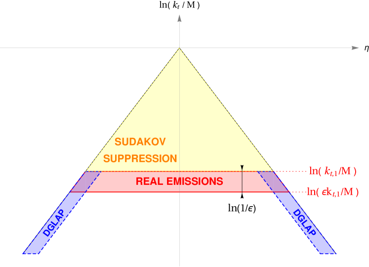
Figure 1: Phase space for a secondary real emission.

In the unresolved region ($k_{ti}<\epsilon k_{t1}$), the DGLAP evolution can be performed inclusively since emissions in this phase-space region do not affect the value of the observable. On the other hand, when $k_{t1}>k_{ti}>\epsilon k_{t1}$ the corresponding hard-collinear emissions modify significantly the observable’s value and therefore must be treated exclusively, namely unintegrated in $k_{t}$.

In addition to the parton densities, starting at ${\cal O}(\alpha_{s})$, one needs to include the coefficient functions that emerge from their renormalisation, and originate from emissions that occur at the edges of the phase space in Fig. 1. The coefficient functions contribute to the logarithmic structure only through the scale of their running coupling, which is the transverse momentum of the emission(s) they are associated with. As done for the parton densities, one can evaluate them initially at a scale $\mu_{0}$ smaller than any transverse momentum in the event, and subsequently evolve them inclusively up to the resolution scale $\epsilon k_{t1}$. Their evolution must be instead treated exclusively in the resolved strip $k_{t1}>k_{ti}>\epsilon k_{t1}$.

In order to introduce the all-order result, it is convenient to simplify the flavour structure of the evolution for the time being. We neglect real-emission kernels that modify the flavour of the emitting leg, namely those that do not have a soft singularity $P_{qg}$ and $P_{gq}$. This ensures that the flavour of the initial parton densities is only modified by the coefficient functions and is conserved by the resolved real radiation. This approximation is made without any loss of generality, and for the only sake of simplicity. The extension to the full flavour case will be trivial once the final formula is obtained.

For the remaining part of the section, it is useful to introduce a matrix notation to simplify the structure of our expressions in flavour space. We define ${\bf f}$ as the array containing the $2n_{f}+1$ partonic densities, where $n_{f}$ denotes the number of active flavours. To handle different Born configurations with different incoming flavours ${c_{\ell}}$, we then define the coefficient-function matrix ${\bf C}^{c_{\ell}}$ as a $(2n_{f}+1)\times(2n_{f}+1)$ diagonal matrix in flavour space whose entries are

$$[{\bf C}^{c_{\ell}}]_{ab}=C_{c_{\ell}f(a)}\delta_{ab},$$ (52)

where $C_{ij}$ are the collinear coefficient functions, $c_{\ell}$ is the flavour of the leg $\ell$ entering the Born process, and $f(a)$ is the flavour corresponding to the $a$-th entry of the parton-density array. For instance, we explicitly show the above convention in the case of Higgs production, considering only a single quark flavour $q$. By defining the array $\mathbf{f}=(f_{g},f_{q},f_{\bar{q}})^{T}$, the matrix ${\bf C}^{g}$ reads

$${\bf C}^{g} = \left(\begin{array}[]{ccc}C_{gg}&0&0\\ 0&C_{gq}&0\\ 0&0&C_{g\bar{q}}\end{array}\right).$$ (56)

The evolution of (52) between two scales is entirely encoded in the evolution of the running coupling. By introducing the corresponding anomalous-dimension matrix ${\bf\Gamma}^{(C)}$

$${\bf\Gamma}^{(C)}(\alpha_{s}(k_{t}))=2\beta(\alpha_{s}(k_{t}))\frac{d\ln{\bf C}^{c_{\ell}}(\alpha_{s}(k_{t}))}{d\alpha_{s}(k_{t})},$$ (57)

we can write the Renormalisation-Group evolution (RGE) of the coefficient function matrix as

$${\bf C}^{c_{\ell}}(\alpha_{s}(\mu))=\exp\left\{-\int_{\mu}^{\mu_{0}}\frac{dk_{t}}{k_{t}}{\bf\Gamma}^{(C)}(\alpha_{s}(k_{t}))\right\}{\bf C}^{c_{\ell}}(\alpha_{s}(\mu_{0})).$$ (58)

In principle, the matrix ${\bf\Gamma}^{(C)}$ should also explicitly carry a label $c_{\ell}$ to specify that it evolves the coefficient function ${\bf C}^{c_{\ell}}$ associated with the Born flavour $c_{\ell}$. We omit this label as the notation in what follows is unambiguous. We stress however that the flavour of the coefficient function is not modified by its RG evolution, indeed it is manifestly flavour diagonal.

The iterative structure of the squared amplitudes appears more transparent if we work in Mellin space, where convolutions become products. We therefore introduce the Mellin transform of a function $g(x)$ as

$$g_{N_{\ell}}\equiv\int_{0}^{1}dx\,x^{N_{\ell}-1}g(x).$$ (59)

The DGLAP Gribov:1972ri ; Altarelli:1977zs ; Dokshitzer:1977sg evolution of the parton-density vector ${\bf f}$ can be conveniently written in Mellin space as

$${\bf f}_{N_{\ell}}(\mu)={\cal P}\exp\left\{-\int_{\mu}^{\mu_{0}}\frac{dk_{t}}{k_{t}}\frac{\alpha_{s}(k_{t})}{\pi}{\bf\Gamma}_{N_{\ell}}(\alpha_{s}(k_{t}))\right\}{\bf f}_{N_{\ell}}(\mu_{0}).$$ (60)

In the previous equation $\cal P$ is the path-ordering symbol, and the matrix ${\bf\Gamma}$ is defined as

$$\left[{\bf\Gamma}_{N_{\ell}}(\alpha_{s}(\mu))\right]_{ab}=\int_{0}^{1}dz\,z^{N_{\ell}-1}\hat{P}_{f(a)f(b)}(z,\alpha_{s}(\mu))\equiv\gamma_{N_{\ell};f(a)f(b)}=\sum_{n=0}^{\infty}\left(\frac{\alpha_{s}(\mu)}{2\pi}\right)^{n}\gamma_{N_{\ell};f(a)f(b)}^{(n)},$$ (61)

where $\hat{P}_{f(a)f(b)}$ are the regularised splitting functions (see Appendix B). We stress that, within the simplifying assumption made above on flavour-conserving real-emission kernels, no splitting functions involving a real quark emission are included, therefore the matrix ${\bf\Gamma}$ is diagonal. Within this assumption, the path ordering in Eq. (60) can be lifted.

With this notation, the hadronic cumulative cross section, differential with respect to the Born phase space $\Phi_{B}$, can be written as

$$\frac{d\Sigma(v)}{d\Phi_{B}}=\int_{{\cal C}_{1}}\frac{dN_{1}}{2\pi i}\int_{{\cal C}_{2}}\frac{dN_{2}}{2\pi i}x_{1}^{-N_{1}}x_{2}^{-N_{2}}\,\sum_{c_{1},c_{2}}\frac{d|M_{B}|_{c_{1}c_{2}}^{2}}{d\Phi_{B}}{\bf f}^{T}_{N_{1}}(\mu_{0})\hat{\bf\Sigma}^{c_{1},c_{2}}_{N_{1},N_{2}}(v){\bf f}_{N_{2}}(\mu_{0}),$$ (62)

where the sum runs over all possible Born configurations and we employed a double inverse Mellin transform. The contours ${\cal C}_{1}$ and ${\cal C}_{2}$ are understood to lie along the imaginary axis to the right of all singularities of the integrand. In Eq. (62), and from now on, we define the notation

$$\frac{d|M_{B}|_{c_{1}c_{2}}^{2}}{d\Phi_{B}}\equiv\int d\Phi^{\prime}_{B}|M_{B}|_{c_{1}c_{2}}^{2}\delta(x_{1}-x_{1}^{\prime})\delta(x_{2}-x_{2}^{\prime})\delta(\Omega_{B}-\Omega_{B}^{\prime})\,,$$

where $\Omega_{B}$ denotes any set of internal phase-space variables used to parametrise the colour-singlet system. The right-hand side differs from the squared amplitude $|M_{B}|_{c_{1}c_{2}}^{2}$ simply by a jacobian factor.

The matrix $\hat{\bf\Sigma}$ encodes the effect of the all-order radiation that evolves the partonic cross section and the corresponding parton densities. To write down an all-order expression for $\hat{\bf\Sigma}$ for the observables (17), we need to iterate the single-emission probability derived in the previous section. Given that the phase space of the $R^{\prime}$ contributions and the exclusive DGLAP evolution steps are completely disentangled in the resolved real radiation, this operation can be performed straightforwardly in Mellin space, yielding

$$\hat{\bf\Sigma}^{c_{1},c_{2}}_{N_{1},N_{2}}(v) =\left[{\bf C}^{c_{1};T}_{N_{1}}(\alpha_{s}(\mu_{0}))H(\mu_{R}){\bf C}^{c_{2}}_{N_{2}}(\alpha_{s}(\mu_{0}))\right]\,\int_{0}^{M}\frac{dk_{t1}}{k_{t1}}\int_{0}^{2\pi}\frac{d\phi_{1}}{2\pi}$$

$$\times e^{-{\bf R}(\epsilon k_{t1})}\exp\left\{-\sum_{\ell=1}^{2}\left(\int_{\epsilon k_{t1}}^{\mu_{0}}\frac{dk_{t}}{k_{t}}\frac{\alpha_{s}(k_{t})}{\pi}{\bf\Gamma}_{N_{\ell}}(\alpha_{s}(k_{t}))+\int_{\epsilon k_{t1}}^{\mu_{0}}\frac{dk_{t}}{k_{t}}{\bf\Gamma}_{N_{\ell}}^{(C)}(\alpha_{s}(k_{t}))\right)\right\}$$

$$\sum_{\ell_{1}=1}^{2}\left({\bf R}_{\ell_{1}}^{\prime}\left(k_{t1}\right)+\frac{\alpha_{s}(k_{t1})}{\pi}{\bf\Gamma}_{N_{\ell_{1}}}(\alpha_{s}(k_{t1}))+{\bf\Gamma}_{N_{\ell_{1}}}^{(C)}(\alpha_{s}(k_{t1}))\right)$$

$$\times\sum_{n=0}^{\infty}\frac{1}{n!}\prod_{i=2}^{n+1}\int_{\epsilon}^{1}\frac{d\zeta_{i}}{\zeta_{i}}\int_{0}^{2\pi}\frac{d\phi_{i}}{2\pi}\sum_{\ell_{i}=1}^{2}\left({\bf R}_{\ell_{i}}^{\prime}\left(k_{ti}\right)+\frac{\alpha_{s}(k_{ti})}{\pi}{\bf\Gamma}_{N_{\ell_{i}}}(\alpha_{s}(k_{ti}))+{\bf\Gamma}_{N_{\ell_{i}}}^{(C)}(\alpha_{s}(k_{ti}))\right)$$

$$\times\Theta\left(v-V(\{\tilde{p}\},k_{1},\dots,k_{n+1})\right),$$ (63)

where now $\zeta_{i}=k_{ti}/k_{t1}$ since we are using the transverse momentum as a resolution and ordering variable. ${\bf R}_{\ell}^{\prime}$ is a diagonal matrix in flavour space: given the flavour $c_{\ell}$ of the Born leg $\ell$, it describes the flavour-conserving resolved radiation off leg $\ell$. It is defined as

$$[{\bf R}_{\ell}^{\prime}]_{ab}=R_{\ell}^{\prime}\delta_{ab},$$ (64)

and $R_{\ell}^{\prime}$ is defined in Eq. (34). The Sudakov operator ${\bf R}$ is then defined as

$${\bf R}(\epsilon k_{t1})=\sum_{\ell=1}^{2}\int_{\epsilon k_{t1}}^{M}\frac{dk_{t}}{k_{t}}{\bf R}_{\ell}^{\prime}(k_{t}).$$ (65)

The terms proportional to ${\bf R}^{\prime}$ in Eq. (2.3.3) encode the contribution of the radiation which is flavour-diagonal, and does not modify the momentum fraction of the incoming partons. This is the analogue of what has been derived in Sec. 2.1 in the case of scale-independent parton densities. In addition, the real emission probability now involves the exclusive evolution for the parton densities and coefficient functions.

The matrices $\hat{\bf\Sigma}^{c_{1},c_{2}}$ are diagonal in flavour space within the flavour assumption that we are making here. The first line of Eq. (2.3.3) contains the factor $\left[{\bf C}^{c_{1};T}_{N_{1}}(\alpha_{s}(\mu_{0}))H(\mu_{R}){\bf C}^{c_{2}}_{N_{2}}(\alpha_{s}(\mu_{0}))\right]$ that encodes the hard-virtual corrections to the form factor and the collinear coefficient functions. Explicit expressions for these quantities will be given later (see Sec. 3.1 and references therein). As discussed above, the coupling of the coefficient functions here is evaluated at $\mu_{0}$ and subsequently evolved up to $\epsilon k_{t1}$ by the operator containing the diagonal matrix ${\bf\Gamma}_{N_{\ell}}^{(C)}$ in the second line of (2.3.3). Similarly, the parton densities are evolved from $\mu_{0}$ up to $\epsilon k_{t1}$. As it was shown in ref. Catani:2010pd , starting at a given order in perturbation theory one needs to include the contribution from the collinear coefficient functions ${\bf G}$, that describe the azimuthal correlations with the initial-state gluons. Such a contribution starts at ${\cal O}(\alpha_{s}^{2})$ (i.e. N³LL) for gluon-fusion processes, and at yet higher orders for quark-initiated ones. It is included in the above formulation by simply adding to Eq. (2.3.3) an analogous term where one makes the replacements

$$\left[{\bf C}^{c_{1};T}_{N_{1}}(\alpha_{s}(\mu_{0}))H(\mu_{R}){\bf C}^{c_{2}}_{N_{2}}(\alpha_{s}(\mu_{0}))\right]\to\left[{\bf G}^{c_{1};T}_{N_{1}}(\alpha_{s}(\mu_{0}))H(\mu_{R}){\bf G}^{c_{2}}_{N_{2}}(\alpha_{s}(\mu_{0}))\right],$$ (66)

and

$${\bf\Gamma}_{N_{\ell}}^{(C)}(\alpha_{s}(k_{t}))\to{\bf\Gamma}_{N_{\ell}}^{(G)}(\alpha_{s}(k_{t})),$$ (67)

where ${\bf\Gamma}_{N_{\ell}}^{(G)}$ is defined analogously to Eq. (57), and the flavour structure of ${\bf G}$ is analogous to the one of the ${\bf C}$ matrix. In what follows this contribution, whenever not reported, is understood.

Eq. (2.3.3) has been derived by iterating the single-emission probability. As discussed above, higher-order logarithmic corrections are simply included by adding higher-order correlated blocks. Specifically, this amounts to including higher-order logarithmic corrections to the radiator $R$ and its derivative $R^{\prime}$, as well as in the anomalous dimensions which drive the evolution of the parton densities and coefficient functions.

We conclude the discussion by pointing out that even if the all-order formulation has been conveniently obtained in Mellin space, it is possible to evaluate Eq. (62) directly in momentum space at any given logarithmic order. We will describe how to do this in Sec. 3.1. Eq. (2.3.3) holds for all inclusive observables (see definition in Sec. 2.3) that do not depend on the rapidity of the initial-state radiation. In the remaining part of this article we specialise to the study of the transverse-momentum case, but analogous conclusions will apply to other observables of the same class.

2.4 Equivalence with impact-parameter-space formulation

In this section we show how to relate our Eq. (62) to the impact-parameter-space formulation of Parisi:1979se . We show the equivalence for the differential partonic cross section (2.3.3) in the case of the transverse momentum $p_{t}$. An analogous proof can be carried out in the case of the $\phi^{*}$.

Our starting point is the differential partonic cross section, where we now set $\mu_{0}=\mu_{R}=M$ without loss of generality:

$$\frac{d}{d^{2}\vec{p}_{t}} \hat{\bf\Sigma}_{N_{1},N_{2}}^{c_{1}c_{2}}(p_{t})={\bf C}^{c_{1};T}_{N_{1}}(\alpha_{s}(M))H(M){\bf C}^{c_{2}}_{N_{2}}(\alpha_{s}(M))\,\int_{0}^{M}\frac{dk_{t1}}{k_{t1}}\int_{0}^{2\pi}\frac{d\phi_{1}}{2\pi}$$

$$\times e^{-{\bf R}(\epsilon k_{t1})}\exp\left\{-\sum_{\ell=1}^{2}\left(\int_{\epsilon k_{t1}}^{M}\frac{dk_{t}}{k_{t}}\frac{\alpha_{s}(k_{t})}{\pi}{\bf\Gamma}_{N_{\ell}}(\alpha_{s}(k_{t}))+\int_{\epsilon k_{t1}}^{M}\frac{dk_{t}}{k_{t}}{\bf\Gamma}_{N_{\ell}}^{(C)}(\alpha_{s}(k_{t}))\right)\right\}$$

$$\times\sum_{\ell_{1}=1}^{2}\left({\bf R}_{\ell_{1}}^{\prime}\left(k_{t1}\right)+\frac{\alpha_{s}(k_{t1})}{\pi}{\bf\Gamma}_{N_{\ell_{1}}}(\alpha_{s}(k_{t1}))+{\bf\Gamma}_{N_{\ell_{1}}}^{(C)}(\alpha_{s}(k_{t1}))\right)$$

$$\times\sum_{n=0}^{\infty}\frac{1}{n!}\prod_{i=2}^{n+1}\int_{\epsilon}^{1}\frac{d\zeta_{i}}{\zeta_{i}}\int_{0}^{2\pi}\frac{d\phi_{i}}{2\pi}\sum_{\ell_{i}=1}^{2}\left({\bf R}_{\ell_{i}}^{\prime}\left(k_{ti}\right)+\frac{\alpha_{s}(k_{ti})}{\pi}{\bf\Gamma}_{N_{\ell_{i}}}(\alpha_{s}(k_{ti}))+{\bf\Gamma}_{N_{\ell_{i}}}^{(C)}(\alpha_{s}(k_{ti}))\right)$$

$$\times\delta^{(2)}\left(\vec{p}_{t}-\left(\vec{k}_{t1}+\dots+\vec{k}_{t(n+1)}\right)\right).$$ (68)

We transform the $\delta$ function into $b$-space as

$$\delta^{(2)}\left(\vec{p}_{t}-\left(\vec{k}_{t1}+\dots+\vec{k}_{t(n+1)}\right)\right)=\int\frac{d^{2}\vec{b}}{4\pi^{2}}e^{-i\vec{b}\cdot\vec{p}_{t}}\prod_{i=1}^{n+1}e^{i\vec{b}\cdot\vec{k}_{ti}},$$ (69)

and we evaluate the azimuthal integrals, which simply amounts to replacing each of the factors $e^{\pm i\vec{b}\cdot\vec{k}_{t}}$ with a Bessel function $J_{0}(bk_{t})$. It is now straightforward to see that the sum in Eq. (2.4) gives rise to an exponential function, yielding

$$\frac{d}{dp_{t}} \hat{\bf\Sigma}_{N_{1},N_{2}}^{c_{1}c_{2}}(p_{t})={\bf C}^{c_{1};T}_{N_{1}}(\alpha_{s}(M))H(M){\bf C}^{c_{2}}_{N_{2}}(\alpha_{s}(M))\,p_{t}\int\!\!b\,dbJ_{0}(p_{t}b)\int_{0}^{M}\frac{dk_{t1}}{k_{t1}}$$

$$\times\sum_{\ell_{1}=1}^{2}\left({\bf R}_{\ell_{1}}^{\prime}\left(k_{t1}\right)+\frac{\alpha_{s}(k_{t1})}{\pi}{\bf\Gamma}_{N_{\ell_{1}}}(\alpha_{s}(k_{t1}))+{\bf\Gamma}_{N_{\ell_{1}}}^{(C)}(\alpha_{s}(k_{t1}))\right)J_{0}(bk_{t1})$$

$$\times\exp\left\{-\sum_{\ell=1}^{2}\int_{k_{t1}}^{M}\frac{dk_{t}}{k_{t}}\left({\bf R}_{\ell}^{\prime}\left(k_{t}\right)+\frac{\alpha_{s}(k_{t})}{\pi}{\bf\Gamma}_{N_{\ell}}(\alpha_{s}(k_{t}))+{\bf\Gamma}_{N_{\ell}}^{(C)}(\alpha_{s}(k_{t}))\right)J_{0}(bk_{t})\right\}$$

$$\times\exp\left\{-\sum_{\ell=1}^{2}\int_{\epsilon k_{t1}}^{M}\frac{dk_{t}}{k_{t}}\left({\bf R}_{\ell}^{\prime}\left(k_{t}\right)+\frac{\alpha_{s}(k_{t})}{\pi}{\bf\Gamma}_{N_{\ell}}(\alpha_{s}(k_{t}))+{\bf\Gamma}_{N_{\ell}}^{(C)}(\alpha_{s}(k_{t}))\right)(1-J_{0}(bk_{t}))\right\}.$$ (70)

We finally notice that we can set $\epsilon\to 0$ in the above formula, given that now the cancellation of divergences is manifest. The $k_{t1}$ integrand is a total derivative and it integrates to one, leaving

$$\frac{d}{dp_{t}} \hat{\bf\Sigma}_{N_{1},N_{2}}^{c_{1}c_{2}}(p_{t})={\bf C}^{c_{1};T}_{N_{1}}(\alpha_{s}(M))H(M){\bf C}^{c_{2}}_{N_{2}}(\alpha_{s}(M))\,p_{t}\int\!\!b\,dbJ_{0}(p_{t}b)$$

$$\times\exp\left\{-\sum_{\ell=1}^{2}\int_{0}^{M}\frac{dk_{t}}{k_{t}}\left({\bf R}_{\ell}^{\prime}\left(k_{t}\right)+\frac{\alpha_{s}(k_{t})}{\pi}{\bf\Gamma}_{N_{\ell}}(\alpha_{s}(k_{t}))+{\bf\Gamma}_{N_{\ell}}^{(C)}(\alpha_{s}(k_{t}))\right)(1-J_{0}(bk_{t}))\right\}.$$ (71)

We now insert the resulting partonic cross section back into the definition of the hadronic cross section (62), and use the second and third terms in the exponent of Eq. (2.4) to evolve the parton densities and the coefficient functions down to $b_{0}/b$, with $b_{0}=2e^{-\gamma_{E}}$. After performing the inverse Mellin transform, and neglecting N⁴LL corrections, we obtain (hereafter we simplify the notation for the parton densities by omitting their $x_{1}$ and $x_{2}$ dependence, which is determined by the Born kinematics $\Phi_{B}$)

$$\frac{d^{2}\Sigma(v)}{d\Phi_{B}dp_{t}} =\sum_{c_{1},c_{2}}\frac{d|M_{B}|_{c_{1}c_{2}}^{2}}{d\Phi_{B}}\int\!\!b\,db\,p_{t}J_{0}(p_{t}b)\,{\bf f}^{T}(b_{0}/b){\bf C}^{c_{1};T}_{N_{1}}(\alpha_{s}(b_{0}/b))H(M){\bf C}^{c_{2}}_{N_{2}}(\alpha_{s}(b_{0}/b)){\bf f}(b_{0}/b)$$

$$\times\exp\left\{-\sum_{\ell=1}^{2}\int_{0}^{M}\frac{dk_{t}}{k_{t}}{\bf R}_{\ell}^{\prime}\left(k_{t}\right)(1-J_{0}(bk_{t}))\right\}.$$ (72)

Eq. (2.4) represents indeed the $b$-space formulation of transverse-momentum resummation. Commonly, it is expressed in the equivalent form Collins:1984kg

$$\frac{d^{2}\Sigma(v)}{d\Phi_{B}dp_{t}} =\sum_{c_{1},c_{2}}\frac{d|M_{B}|_{c_{1}c_{2}}^{2}}{d\Phi_{B}}\int\!\!b\,db\,p_{t}J_{0}(p_{t}b)\,{\bf f}^{T}(b_{0}/b){\bf C}^{c_{1};T}_{N_{1}}(\alpha_{s}(b_{0}/b))H_{\text{\scriptsize CSS}}(M){\bf C}^{c_{2}}_{N_{2}}(\alpha_{s}(b_{0}/b)){\bf f}(b_{0}/b)$$

$$\times\exp\left\{-\sum_{\ell=1}^{2}\int_{0}^{M}\frac{dk_{t}}{k_{t}}{\bf R}_{\text{\scriptsize CSS},\ell}^{\prime}\left(k_{t}\right)\Theta(k_{t}-\frac{b_{0}}{b})\right\}.$$ (73)

where ${\bf R}_{\text{\scriptsize CSS},\ell}^{\prime}$ and $H_{\text{\scriptsize CSS}}(M)$ are the Sudakov and hard function commonly used for a $b$-space formulation Collins:1984kg . As shown in ref. Catani:2010pd , and as already stressed above, both Eqs. (2.4) and (2.4) receive an extra contribution due to the azimuthal correlations which are parametrised by the ${\bf G}$ coefficient functions. We omit them in this comparison for the sake of simplicity, however it is clear that analogous considerations apply in that case. The comparison between Eqs. (2.4) and (2.4) allows us to extract the N³LL ingredients from the latter formulation as obtained in refs. Catani:2011kr ; Catani:2012qa ; Li:2016ctv ; Vladimirov:2016dll , that will be reported in the next section.

We start by using the relation

$$(1-J_{0}(bk_{t}))\simeq\Theta(k_{t}-\frac{b_{0}}{b})+\frac{\zeta_{3}}{12}\frac{\partial^{3}}{\partial\ln(Mb/b_{0})^{3}}\Theta(k_{t}-\frac{b_{0}}{b})+\dots,$$ (74)

where we ignored N⁴LL terms. In the above formula the derivative in the second term of the right-hand-side is meant to act on the integral whose bounds are set by $\Theta(k_{t}-\frac{b_{0}}{b})$. This yields, at N³LL,

$$\frac{d^{2}\Sigma(v)}{d\Phi_{B}dp_{t}} =\sum_{c_{1},c_{2}}\frac{d|M_{B}|_{c_{1}c_{2}}^{2}}{d\Phi_{B}}\int\!\!b\,db\,p_{t}J_{0}(p_{t}b)\,{\bf f}^{T}(b_{0}/b){\bf C}^{c_{1};T}_{N_{1}}(\alpha_{s}(b_{0}/b))H(M){\bf C}^{c_{2}}_{N_{2}}(\alpha_{s}(b_{0}/b)){\bf f}(b_{0}/b)$$

$$\times\exp\left\{-\sum_{\ell=1}^{2}\left(\int_{b_{0}/b}^{M}\frac{dk_{t}}{k_{t}}{\bf R}_{\ell}^{\prime}\left(k_{t}\right)+\frac{\zeta_{3}}{12}\frac{\partial^{3}}{\partial\ln(Mb/b_{0})^{3}}\int_{b_{0}/b}^{M}\frac{dk_{t}}{k_{t}}{\bf R}_{\ell}^{\prime}\left(k_{t}\right)\right)\right\}.$$ (75)

The second term in the exponent of Eq. (2.4) starts at N³LL, so up to NNLL the two definitions (the one in terms of a $J_{0}$ and the one in terms of the theta function) are manifestly equivalent. To relate the two formulations we recall the definition of ${\bf R}^{\prime}$ in Eq. (64) and we express the Sudakov radiators as (65)

$$R(b) =\sum_{\ell=1}^{2}\int_{b_{0}/b}^{M}\frac{dk_{t}}{k_{t}}R_{\ell}^{\prime}\left(k_{t}\right)=\sum_{\ell=1}^{2}\int_{b_{0}/b}^{M}\frac{dk_{t}}{k_{t}}\left(A_{\ell}(\alpha_{s}(k_{t}))\ln\frac{M^{2}}{k_{t}^{2}}+B_{\ell}(\alpha_{s}(k_{t}))\right)$$

$$R_{\text{\scriptsize CSS}}(b) =\sum_{\ell=1}^{2}\int_{b_{0}/b}^{M}\frac{dk_{t}}{k_{t}}{R}_{\text{\scriptsize CSS},\ell}^{\prime}\left(k_{t}\right)=\sum_{\ell=1}^{2}\int_{b_{0}/b}^{M}\frac{dk_{t}}{k_{t}}\left(A_{\text{\scriptsize CSS},\ell}(\alpha_{s}(k_{t}))\ln\frac{M^{2}}{k_{t}^{2}}+B_{\text{\scriptsize CSS},\ell}(\alpha_{s}(k_{t}))\right).$$ (76)

The anomalous dimensions $A_{\ell}$ and $B_{\ell}$ relative to leg $\ell$ and the hard function $H$ admit an expansion in the strong coupling as

$$A_{\ell}(\alpha_{s})=\sum_{n=1}^{4}\left(\frac{\alpha_{s}}{2\pi}\right)^{n}A^{(n)}_{\ell},\,\quad B_{\ell}(\alpha_{s})=\sum_{n=1}^{3}\left(\frac{\alpha_{s}}{2\pi}\right)^{n}B^{(n)}_{\ell},\quad H(M)=1+\sum_{n=1}^{2}\left(\frac{\alpha_{s}(M)}{2\pi}\right)^{n}H^{(n)}(M).$$ (77)

The relation between the coefficients that enter at N³LL can be deducted by equating Eqs. (2.4) and (2.4), obtaining

$$A_{\ell}^{(4)} =A_{\text{\scriptsize CSS},\ell}^{(4)}-32A^{(1)}_{\ell}\pi^{3}\beta_{0}^{3}\zeta_{3},$$

$$B_{\ell}^{(3)} =B_{\text{\scriptsize CSS},\ell}^{(3)}-16A^{(1)}_{\ell}\pi^{2}\beta_{0}^{2}\zeta_{3},$$

$$H^{(2)}(M) =H_{\text{\scriptsize CSS}}^{(2)}(M)+\frac{8}{3}\pi\beta_{0}\zeta_{3}\left(\frac{1}{2}\sum_{\ell=1}^{2}A^{(1)}_{\ell}\right).$$ (78)

The above equations constitute the ingredients for our N³LL resummation. Physically, the extra terms proportional to $\zeta_{3}$ arise from the fact that the ${\cal O}(\alpha_{s}^{2})$ terms proportional to $\delta(1-z)$ in the coefficient functions in momentum space differ from their $b$-space counterpart. This difference precisely amounts to the new contributions in Eqs. (2.4). We stress that only the combination of $A_{\ell}^{(4)}$, $B_{\ell}^{(3)}$, $H^{(2)}$ and $C^{(2)}$ is resummation-scheme invariant, hence our choice of absorbing the new terms into $A_{\ell}^{(4)}$, $B_{\ell}^{(3)}$, $H^{(2)}$ is indeed arbitrary. One could analogously define an alternative scheme in which the extra terms are directly absorbed into the ${\cal O}(\alpha_{s}^{2})$ coefficient functions, thus leaving the two-loop form factor unchanged.

3 Evaluation up to N³LL

In this section we evaluate our all-order master formulae (62) and (2.3.3) explicitly up to N³LL accuracy. The latter equations can already be evaluated as they are by means of Monte Carlo techniques; however, at any given logarithmic order it is possible, and convenient, to further manipulate them in order to evaluate them directly in momentum space, without the need of the Mellin transform.

3.1 Momentum-space formulation

We firstly focus on the partonic cross section (2.3.3). There are three main ingredients: the Sudakov radiator and its derivative, the block containing coefficient functions $C(\alpha_{s})$ and hard-virtual corrections to the form factor $H(\mu_{R})$, and the anomalous dimensions that rule the evolution of parton densities and coefficient functions.

For colour-singlet production, the coefficients entering the Sudakov radiator satisfy $A^{(n)}_{1}=A^{(n)}_{2}=A^{(n)}$, and $B^{(n)}_{1}=B^{(n)}_{2}=B^{(n)}$. Coefficients $A^{(1)}$, $A^{(2)}$, $A^{(3)}$, $B^{(1)}$, $B^{(2)}$ have been known for several years deFlorian:2001zd ; Davies:1984hs ; Becher:2010tm , and they are collected, for instance, in the appendix of ref. Banfi:2012jm . The N³LL coefficient $B^{(3)}$ can be extracted from the recent result Li:2016ctv ; Vladimirov:2016dll . For gluon processes it reads:

$$B^{(3)} =C_{A}^{3}\left(\frac{22\zeta_{3}\zeta_{2}}{3}-\frac{799\zeta_{2}}{81}-\frac{5\pi^{2}\zeta_{3}}{9}-\frac{2533\zeta_{3}}{54}-\frac{77\zeta_{4}}{12}+20\zeta_{5}-\frac{319\pi^{4}}{1080}+\frac{6109\pi^{2}}{1944}+\frac{34219}{1944}\right)$$

$$+C_{A}^{2}n_{f}\left(\frac{103\zeta_{2}}{81}+\frac{202\zeta_{3}}{27}-\frac{5\zeta_{4}}{6}+\frac{41\pi^{4}}{540}-\frac{599\pi^{2}}{972}-\frac{10637}{1944}\right)+C_{A}C_{F}n_{f}\left(2\zeta_{4}-\frac{\pi^{4}}{45}-\frac{\pi^{2}}{12}+\frac{241}{72}\right)$$

$$-\frac{1}{4}C_{F}^{2}n_{f}+C_{A}n_{f}^{2}\left(-\frac{2\zeta_{3}}{27}+\frac{5\pi^{2}}{162}+\frac{529}{1944}\right)-\frac{11}{36}C_{F}n_{f}^{2}-32C_{A}\pi^{2}\beta_{0}^{2}\zeta_{3}$$

$$\approx-492.908-32C_{A}\pi^{2}\beta_{0}^{2}\zeta_{3},$$ (79)

while for quark processes

$$B^{(3)} =C_{A}^{2}C_{F}\left(\frac{22\zeta_{3}\zeta_{2}}{3}-\frac{799\zeta_{2}}{81}-\frac{11\pi^{2}\zeta_{3}}{9}+\frac{2207\zeta_{3}}{54}-\frac{77\zeta_{4}}{12}-10\zeta_{5}-\frac{83\pi^{4}}{360}-\frac{7163\pi^{2}}{1944}+\frac{151571}{3888}\right)$$

$$+C_{F}^{3}\left(\frac{4\pi^{2}\zeta_{3}}{3}-17\zeta_{3}+60\zeta_{5}-\frac{2\pi^{4}}{5}-\frac{3\pi^{2}}{4}-\frac{29}{8}\right)+C_{F}^{2}n_{f}\left(\frac{34\zeta_{3}}{3}+2\zeta_{4}-\frac{7\pi^{4}}{54}-\frac{13\pi^{2}}{36}+\frac{23}{4}\right)$$

$$+C_{A}C_{F}^{2}\left(-\frac{2}{3}\pi^{2}\zeta_{3}-\frac{211\zeta_{3}}{3}-30\zeta_{5}+\frac{247\pi^{4}}{540}+\frac{205\pi^{2}}{36}-\frac{151}{16}\right)$$

$$+C_{A}C_{F}n_{f}\left(\frac{103\zeta_{2}}{81}-\frac{128\zeta_{3}}{27}-\frac{5\zeta_{4}}{6}+\frac{11\pi^{4}}{180}+\frac{1297\pi^{2}}{972}-\frac{3331}{243}\right)+C_{F}n_{f}^{2}\left(\frac{10\zeta_{3}}{27}-\frac{5\pi^{2}}{54}+\frac{1115}{972}\right)$$

$$-32C_{F}\pi^{2}\beta_{0}^{2}\zeta_{3}\approx-116.685-32C_{F}\pi^{2}\beta_{0}^{2}\zeta_{3}.$$ (80)

The remaining N³LL anomalous dimension $A^{(4)}$ is currently incomplete given that the four-loop cusp anomalous dimension is still unknown. Here we compute $A^{(4)}$ according to Eq. (71) of ref. Becher:2010tm or Eq. (4.6) of ref. Monni:2011gb , using the results of refs. Li:2016ctv ; Vladimirov:2016dll for the soft anomalous dimension, and setting the four-loop cusp anomalous dimension to zero. For gluon-initiated processes we get

$$A^{(4)} =C_{A}^{4}\left(\frac{121}{3}\zeta_{3}\zeta_{2}-\frac{8789\zeta_{2}}{162}-\frac{19093\zeta_{3}}{54}-\frac{847\zeta_{4}}{24}+132\zeta_{5}+\frac{3761815}{11664}\right)$$

$$+C_{A}^{3}n_{f}\left(-\frac{22}{3}\zeta_{3}\zeta_{2}+\frac{2731\zeta_{2}}{162}+\frac{4955\zeta_{3}}{54}+\frac{11\zeta_{4}}{6}-24\zeta_{5}-\frac{31186}{243}\right)$$

$$+C_{A}^{2}C_{F}n_{f}\left(\frac{272\zeta_{3}}{9}+11\zeta_{4}-\frac{7351}{144}\right)+C_{A}^{2}n_{f}^{2}\left(-\frac{103\zeta_{2}}{81}-\frac{47\zeta_{3}}{27}+\frac{5\zeta_{4}}{6}+\frac{13819}{972}\right)$$

$$+C_{A}C_{F}n_{f}^{2}\left(-\frac{38\zeta_{3}}{9}-2\zeta_{4}+\frac{215}{24}\right)+C_{A}n_{f}^{3}\left(-\frac{4\zeta_{3}}{9}-\frac{232}{729}\right)-64C_{A}\pi^{3}\beta_{0}^{3}\zeta_{3}$$

$$\approx-2675.68-64C_{A}\pi^{3}\beta_{0}^{3}\zeta_{3},$$ (81)

while for quark-initiated ones

$$A^{(4)} =C_{A}^{3}C_{F}\left(\frac{121}{3}\zeta_{3}\zeta_{2}-\frac{8789\zeta_{2}}{162}-\frac{19093\zeta_{3}}{54}-\frac{847\zeta_{4}}{24}+132\zeta_{5}+\frac{3761815}{11664}\right)$$

$$+C_{A}^{2}C_{F}n_{f}\left(-\frac{22}{3}\zeta_{3}\zeta_{2}+\frac{2731\zeta_{2}}{162}+\frac{4955\zeta_{3}}{54}+\frac{11\zeta_{4}}{6}-24\zeta_{5}-\frac{31186}{243}\right)$$

$$+C_{A}C_{F}^{2}n_{f}\left(\frac{272\zeta_{3}}{9}+11\zeta_{4}-\frac{7351}{144}\right)+C_{A}C_{F}n_{f}^{2}\left(-\frac{103\zeta_{2}}{81}-\frac{47\zeta_{3}}{27}+\frac{5\zeta_{4}}{6}+\frac{13819}{972}\right)$$

$$+C_{F}^{2}n_{f}^{2}\left(-\frac{38\zeta_{3}}{9}-2\zeta_{4}+\frac{215}{24}\right)+C_{F}n_{f}^{3}\left(-\frac{4\zeta_{3}}{9}-\frac{232}{729}\right)-64C_{F}\pi^{3}\beta_{0}^{3}\zeta_{3}$$

$$\approx-1189.19-64C_{F}\pi^{3}\beta_{0}^{3}\zeta_{3}.$$ (82)

We have left the additional terms arising from Eq. (2.4) unexpanded to facilitate the comparison to the existing literature. The remaining quantities are evaluated with $n_{f}=5$. The expression of the Sudakov radiator is analogous to the $b$-space one, i.e.

$$R(\epsilon k_{t1}) =\sum_{\ell=1}^{2}\int_{\epsilon k_{t1}}^{M}\frac{dk_{t}}{k_{t}}R_{\ell}^{\prime}\left(k_{t}\right)=\sum_{\ell=1}^{2}\int_{\epsilon k_{t1}}^{M}\frac{dk_{t}}{k_{t}}\left(A_{\ell}(\alpha_{s}(k_{t}))\ln\frac{M^{2}}{k_{t}^{2}}+B_{\ell}(\alpha_{s}(k_{t}))\right),$$ (83)

and, as above, we define $R^{\prime}$ as the logarithmic derivative of $R$

$$R^{\prime}_{\ell}(k_{t1})=\frac{dR_{\ell}(k_{t1})}{dL},$$ (84)

where we defined

$$L=\ln\frac{M}{k_{t1}}.$$ (85)

In order to make the numerical evaluation of our master formula Eq. (2.3.3) more efficient, we can make a further approximation on the integrand without spoiling the logarithmic accuracy of the result. Before we describe the procedure in detail, we stress that this additional manipulation is not strictly necessary and one could in principle implement directly Eq. (2.3.3) in a Monte-Carlo program.

Since the ratios $k_{ti}/k_{t1}$ for all resolved blocks are of order 1, we can expand $R$ and its derivative about $k_{t1}$, retaining terms that contribute at the desired logarithmic accuracy. At N³LL one has

$$R(\epsilon k_{t1}) =R(k_{t1})+R^{\prime}(k_{t1})\ln\frac{1}{\epsilon}+\frac{1}{2!}R^{\prime\prime}(k_{t1})\ln^{2}\frac{1}{\epsilon}+\frac{1}{3!}R^{\prime\prime\prime}(k_{t1})\ln^{3}\frac{1}{\epsilon}+\dots$$

$$R^{\prime}(k_{ti}) =R^{\prime}(k_{t1})+R^{\prime\prime}(k_{t1})\ln\frac{1}{\zeta_{i}}+\frac{1}{2!}R^{\prime\prime\prime}(k_{t1})\ln^{2}\frac{1}{\zeta_{i}}+\dots,$$ (86)

where the dots denote N⁴LL terms, and we have employed the usual notation $\zeta_{i}=k_{ti}/k_{t1}$.

We recall that the transverse momenta of blocks in the resolved ensemble are parametrically of the same order. This is because rIRC safety ensures that blocks $k$ with $k_{t}\ll k_{t1}$ do not contribute to the observable and are encoded in the Sudakov radiator. Therefore, since $\ln(1/\zeta_{i})$ in the above formula is the logarithm of an ${\cal O}(1)$ quantity, each term in the right-hand-side of Eq. (3.1) is logarithmically subleading with respect to the one to its left.

The logarithms $\ln(1/\epsilon)$ in the first line of Eq. (3.1) are a parametrisation of the IRC divergences arising from the combination of real-unresolved blocks and virtual corrections, expanded at a given logarithmic order. The $\epsilon$ dependence exactly cancels against the corresponding terms in the resolved real corrections (denoted by the same-order derivative of $R$) upon integration over $\zeta_{i}$, as it will be shown below. This is a convenient way to recast the subtraction of IRC divergences at each logarithmic order in our formulation.

The terms proportional to $R^{\prime}(k_{t1})$ are to be retained starting at NLL, those proportional to $R^{\prime\prime}(k_{t1})$ contribute at NNLL and, finally, the ones proportional to $R^{\prime\prime\prime}(k_{t1})$ are needed at N³LL. Starting from the NLL ensemble, we note that correcting a single block with respect to its $R^{\prime}(k_{t1})$ approximation (i.e. including for that block the subleading terms of Eq. (3.1)) gives rise at most to a NNLL correction of order ${\cal O}(\alpha_{s}^{n}L^{n-1})$ in our counting. Modifying two blocks would lead to a relative correction of order ${\cal O}(\alpha_{s}^{n}L^{n-2})$, i.e. N³LL, and so on. Therefore, at any given logarithmic order, it is sufficient to keep terms beyond the $R^{\prime}(k_{t1})$ approximation only for a finite number of blocks (namely a single block at NNLL, two blocks at N³LL, and so forth). Consistently, one has to expand out the corresponding terms in the Sudakov that cancel the $\epsilon$ divergences of the modified real blocks to the given logarithmic order. This prescription has been derived and discussed in detail at NNLL in ref. Banfi:2014sua , and will be used later in this section.

As a next step we address the evolution of the parton densities and relative coefficient functions encoded in Eq. (2.3.3), whose anomalous dimensions $\Gamma_{N}$ and $\Gamma_{N}^{(C)}$ have been defined in Eqs. (60), and (58). Only a finite number of terms in their perturbative series needs to be retained at a given logarithmic accuracy: in particular, contributions from the ${\cal O}(\alpha_{s}^{n})$ term in $\Gamma_{N}$ enter for a Nⁿ⁺¹LL resummation (we recall that the series of $\Gamma_{N}$ starts at ${\cal O}(\alpha_{s}^{0})$, hence these terms start contributing at NLL). On the other hand, the contribution of the coefficient functions, and therefore of the corresponding anomalous dimension, starts at NNLL. Therefore the ${\cal O}(\alpha_{s}^{m})$ term in $\Gamma_{N}^{(C)}$ is necessary at N^m+1LL, since its expansion starts at ${\cal O}(\alpha_{s})$.

We can then perform the same expansion about $k_{t1}$ for the terms in Eq. (2.3.3) containing ${\bf\Gamma}$ and ${\bf\Gamma}^{(C)}$. Up to N³LL we expand the exponent of the evolution operators as

$$\int_{\epsilon k_{t1}}^{\mu_{0}}\frac{dk_{t}}{k_{t}}\frac{\alpha_{s}(k_{t})}{\pi}{\bf\Gamma}_{N_{\ell}}(\alpha_{s}(k_{t})) =\int_{k_{t1}}^{\mu_{0}}\frac{dk_{t}}{k_{t}}\frac{\alpha_{s}(k_{t})}{\pi}{\bf\Gamma}_{N_{\ell}}(\alpha_{s}(k_{t}))+\frac{d}{dL}\int_{k_{t1}}^{\mu_{0}}\frac{dk_{t}}{k_{t}}\frac{\alpha_{s}(k_{t})}{\pi}{\bf\Gamma}_{N_{\ell}}(\alpha_{s}(k_{t}))\ln\frac{1}{\epsilon}$$

$$+\frac{1}{2}\frac{d^{2}}{dL^{2}}\int_{k_{t1}}^{\mu_{0}}\frac{dk_{t}}{k_{t}}\frac{\alpha_{s}(k_{t})}{\pi}{\bf\Gamma}_{N_{\ell}}(\alpha_{s}(k_{t}))\ln^{2}\frac{1}{\epsilon}+\dots$$ (87)

$$\int_{\epsilon k_{t1}}^{\mu_{0}}\frac{dk_{t}}{k_{t}}{\bf\Gamma}_{N_{\ell}}^{(C)}(\alpha_{s}(k_{t})) =\int_{k_{t1}}^{\mu_{0}}\frac{dk_{t}}{k_{t}}{\bf\Gamma}_{N_{\ell}}^{(C)}(\alpha_{s}(k_{t}))+\frac{d}{dL}\int_{k_{t1}}^{\mu_{0}}\frac{dk_{t}}{k_{t}}{\bf\Gamma}_{N_{\ell}}^{(C)}(\alpha_{s}(k_{t}))\ln\frac{1}{\epsilon}+\dots,$$ (88)

and the corresponding resolved real-emission kernels as

$$\frac{\alpha_{s}(k_{tj})}{\pi}{\bf\Gamma}_{N_{\ell}}(\alpha_{s}(k_{tj})) =\frac{\alpha_{s}(k_{t1})}{\pi}{\bf\Gamma}_{N_{\ell}}(\alpha_{s}(k_{t1}))+\frac{d}{dL}\frac{\alpha_{s}(k_{t1})}{\pi}{\bf\Gamma}_{N_{\ell}}(\alpha_{s}(k_{t1}))\ln\frac{1}{\zeta_{j}}+\dots$$ (89)

$${\bf\Gamma}_{N_{\ell}}^{(C)}(\alpha_{s}(k_{tj})) ={\bf\Gamma}_{N_{\ell}}^{(C)}(\alpha_{s}(k_{t1}))+\dots,$$ (90)

where as usual $L=\ln(M/k_{t1})$. The first terms on the right-hand side of Eqs. (87), and (88) represent the evolution operator that runs the parton densities and the coefficient functions, respectively, from $\mu_{0}$ up to $k_{t1}$. The remaining terms describe the exclusive evolution of the parton densities and of the coefficient functions in the resolved strip. In particular, the $\epsilon$-dependent terms completely cancel against the corresponding terms in the real-emission kernel of Eqs. (89), and (90) upon integration over the resolved-radiation phase space.

At NLL the coefficient functions are an identity matrix in flavour space, and therefore their evolution operator is trivial. The contribution of the ${\bf\Gamma}_{N}$ in the exponent starts at NLL, while the exclusive evolution of the parton densities in the resolved strip starts at NNLL since it corresponds to emissions in the hard-collinear edge of the phase space. Therefore, at NLL one only needs to retain the first term in the right-hand side of Eq. (87), and ignore everything else in Eqs. (87), (88), (89), and (90), which corresponds to evaluating the parton densities at $\mu_{F}=k_{t1}$. At this order, the evolution can be carried out by means of the tree-level anomalous dimension $\gamma^{(0)}_{N}$.

Similarly, at NNLL one needs to take into account the second term in the r.h.s. of Eq. (87) and the first term in the r.h.s. of Eq. (89), where now the anomalous dimension ${\bf\Gamma}_{N}$ is evaluated at one-loop accuracy (i.e. including $\gamma_{N}^{(1)}$). At this order also the coefficient functions start contributing with their inclusive evolution, therefore one needs to add the first term in the r.h.s. of Eq. (88). The corresponding exclusive evolution of the coefficient functions in the resolved strip, encoded in the r.h.s. of Eq. (90) only starts at N³LL. At higher orders, one simply needs to add subsequent terms from the above equations, and evaluate the anomalous dimensions at the appropriate perturbative accuracy.

As discussed above for the Sudakov radiator, at any given logarithmic order beyond NLL, it is sufficient to include the extra $\epsilon$-dependent terms from Eqs. (87), (88) in the exponent, and the corresponding terms in the resolved real radiation from Eqs. (89), (90) only for a finite number of emissions, namely a single emission at NNLL, two emissions at N³LL, and so forth.

Finally, we need to deal with the block ${\bf C}^{c_{1};T}_{N_{1}}(\alpha_{s}(\mu_{0}))H(\mu_{R}){\bf C}^{c_{2}}_{N_{2}}(\alpha_{s}(\mu_{0}))$ in Eq. (2.3.3). As discussed in the previous section, for a generic process this block receives a contribution from the gluon collinear correlations ${\bf G}$, as in Eq. (67). Since the contribution of the ${\bf G}$ functions starts at N³LL, at this order one can drop the $\epsilon$ dependence in their evolution; namely, in the analogue of Eq. (88) with ${\bf\Gamma}_{N}^{(C)}\to{\bf\Gamma}_{N}^{(G)}$, only the first term on the right-hand side needs to be retained. This amounts to evaluating the coupling of the ${\bf G}$ coefficient functions at $k_{t1}$.

With the expansions detailed above, Eq. (2.3.3) becomes

$$\hat{\bf\Sigma}_{N_{1},N_{2}}^{c_{1}c_{2}}(v)={\bf C}^{c_{1};T}_{N_{1}}(\alpha_{s}(\mu_{0}))H(\mu_{R}){\bf C}^{c_{2}}_{N_{2}}(\alpha_{s}(\mu_{0}))\,\int_{0}^{M}\frac{dk_{t1}}{k_{t1}}\int_{0}^{2\pi}\frac{d\phi_{1}}{2\pi}$$

$$\times e^{-{\bf R}(k_{t1})-{\bf R}^{\prime}(k_{t1})\ln\frac{1}{\epsilon}-\frac{1}{2!}{\bf R}^{\prime\prime}(k_{t1})\ln^{2}\frac{1}{\epsilon}-\frac{1}{3!}{\bf R}^{\prime\prime\prime}(k_{t1})\ln^{3}\frac{1}{\epsilon}+\dots}$$

$$\times\exp\left\{-\sum_{\ell=1}^{2}\left(\int_{k_{t1}}^{\mu_{0}}\frac{dk_{t}}{k_{t}}\frac{\alpha_{s}(k_{t})}{\pi}{\bf\Gamma}_{N_{\ell}}(\alpha_{s}(k_{t}))+\frac{d}{dL}\int_{k_{t1}}^{\mu_{0}}\frac{dk_{t}}{k_{t}}\frac{\alpha_{s}(k_{t})}{\pi}{\bf\Gamma}_{N_{\ell}}(\alpha_{s}(k_{t}))\ln\frac{1}{\epsilon}\right.\right.$$

$$\left.\left.\hskip 28.45274pt+\frac{1}{2!}\frac{d^{2}}{dL^{2}}\int_{k_{t1}}^{\mu_{0}}\frac{dk_{t}}{k_{t}}\frac{\alpha_{s}(k_{t})}{\pi}{\bf\Gamma}_{N_{\ell}}(\alpha_{s}(k_{t}))\ln^{2}\frac{1}{\epsilon}+\dots\right.\right.$$

$$\left.\hskip 28.45274pt+\int_{k_{t1}}^{\mu_{0}}\frac{dk_{t}}{k_{t}}{\bf\Gamma}_{N_{\ell}}^{(C)}(\alpha_{s}(k_{t}))+\frac{d}{dL}\int_{k_{t1}}^{\mu_{0}}\frac{dk_{t}}{k_{t}}{\bf\Gamma}_{N_{\ell}}^{(C)}(\alpha_{s}(k_{t}))\ln\frac{1}{\epsilon}+\dots\right)\Bigg{\}}$$

$$\times\sum_{\ell_{1}=1}^{2}\left({\bf R}_{\ell_{1}}^{\prime}\left(k_{t1}\right)+\frac{\alpha_{s}(k_{t1})}{\pi}{\bf\Gamma}_{N_{\ell_{1}}}(\alpha_{s}(k_{t1}))+{\bf\Gamma}_{N_{\ell_{1}}}^{(C)}(\alpha_{s}(k_{t1}))\right)$$

$$\times\sum_{n=0}^{\infty}\frac{1}{n!}\prod_{i=2}^{n+1}\int_{\epsilon}^{1}\frac{d\zeta_{i}}{\zeta_{i}}\int_{0}^{2\pi}\frac{d\phi_{i}}{2\pi}\sum_{\ell_{i}=1}^{2}\Bigg{\{}{\bf R}_{\ell_{i}}^{\prime}\left(k_{t1}\right)+{\bf R}_{\ell_{i}}^{\prime\prime}\left(k_{t1}\right)\ln\frac{1}{\zeta_{i}}+\frac{1}{2}{\bf R}_{\ell_{i}}^{\prime\prime\prime}\left(k_{t1}\right)\ln^{2}\frac{1}{\zeta_{i}}+\dots$$

$$+\frac{\alpha_{s}(k_{t1})}{\pi}{\bf\Gamma}_{N_{\ell_{i}}}(\alpha_{s}(k_{t1}))+\frac{d}{dL}\left(\frac{\alpha_{s}(k_{t1})}{\pi}{\bf\Gamma}_{N_{\ell_{i}}}(\alpha_{s}(k_{t1}))\right)\ln\frac{1}{\zeta_{i}}+\dots$$

$$+{\bf\Gamma}_{N_{\ell_{i}}}^{(C)}(\alpha_{s}(k_{t1}))+\dots\Bigg{\}}\Theta\left(v-V(\{\tilde{p}\},k_{1},\dots,k_{n+1})\right)+\{{\bf C}\to{\bf G};{\bf\Gamma}^{(C)}\to{\bf\Gamma}^{(G)}\}\,.$$ (91)

Following the procedure of ref. Banfi:2014sua , we can express the $\ln(1/\epsilon)$ singularities in the exponent of Eq. (3.1) as integrals over dummy real emissions as follows

$$\ln\frac{1}{\epsilon}=\int_{\epsilon}^{1}\frac{d\zeta}{\zeta},\qquad\quad\frac{1}{2}\ln^{2}\frac{1}{\epsilon}=\int_{\epsilon}^{1}\frac{d\zeta}{\zeta}\ln\frac{1}{\zeta},\qquad\quad\frac{1}{3!}\ln^{3}\frac{1}{\epsilon}=\frac{1}{2}\int_{\epsilon}^{1}\frac{d\zeta}{\zeta}\ln^{2}\frac{1}{\zeta},$$ (92)

and subsequently expand out the divergent part of the exponent, retaining the terms necessary at a given logarithmic order. We further introduce the average of a function $G(\{\tilde{p}\},\{k_{i}\})$ over the measure $d{\cal Z}$

$$\begin{split}\int d{\cal Z}[\{R^{\prime},k_{i}\}]G(\{\tilde{p}\},\{k_{i}\})=\epsilon^{R^{\prime}(k_{t1})}\sum_{n=0}^{\infty}\frac{1}{n!}\prod_{i=2}^{n+1}\int_{\epsilon}^{1}\frac{d\zeta_{i}}{\zeta_{i}}\int_{0}^{2\pi}\frac{d\phi_{i}}{2\pi}R^{\prime}(k_{t1})G(\{\tilde{p}\},k_{1},\dots,k_{n+1})\,,\end{split}$$ (93)

where we simplified the notation by using

$$R^{\prime}(k_{t1})=\sum_{\ell=1,2}R^{\prime}_{\ell}(k_{t1}).$$ (94)

The dependence on the regulator $\epsilon$ cancels exactly in Eq. (93).

We can plug Eq. (3.1) into the definition of the hadronic cross section (62). We define the derivatives of the parton densities by means of the DGLAP evolution equation

$$\frac{\partial f(\mu,x)}{\partial\ln\mu}=\frac{\alpha_{s}(\mu)}{\pi}\int_{x}^{1}\frac{dz}{z}\hat{P}(z,\alpha_{s}(\mu))f(\mu,\frac{x}{z}),$$ (95)

where $\hat{P}(z,\alpha_{s}(\mu))$ is the regularised splitting function

$$\hat{P}(z,\alpha_{s}(\mu))=\hat{P}^{(0)}(z)+\frac{\alpha_{s}(\mu)}{2\pi}\hat{P}^{(1)}(z)+\left(\frac{\alpha_{s}(\mu)}{2\pi}\right)^{2}\hat{P}^{(2)}(z)+\dots$$ (96)

Moreover, we introduce the following parton luminosities

$${\cal L}_{\rm NLL}(k_{t1})=\sum_{c,c^{\prime}}\frac{d|M_{B}|_{cc^{\prime}}^{2}}{d\Phi_{B}}f_{c}\!\left(k_{t1},x_{1}\right)f_{c^{\prime}}\!\left(k_{t1},x_{2}\right),$$ (97)

$${\cal L}_{\rm NNLL}(k_{t1})=\sum_{c,c^{\prime}}\frac{d|M_{B}|_{cc^{\prime}}^{2}}{d\Phi_{B}}\sum_{i,j}\int_{x_{1}}^{1}\frac{dz_{1}}{z_{1}}\int_{x_{2}}^{1}\frac{dz_{2}}{z_{2}}f_{i}\!\left(k_{t1},\frac{x_{1}}{z_{1}}\right)f_{j}\!\left(k_{t1},\frac{x_{2}}{z_{2}}\right)$$

$$\Bigg{(}\delta_{ci}\delta_{c^{\prime}j}\delta(1-z_{1})\delta(1-z_{2})\left(1+\frac{\alpha_{s}(\mu_{R})}{2\pi}H^{(1)}(\mu_{R})\right)$$

$$+\frac{\alpha_{s}(\mu_{R})}{2\pi}\frac{1}{1-2\alpha_{s}(\mu_{R})\beta_{0}L}\left(C_{ci}^{(1)}(z_{1})\delta(1-z_{2})\delta_{c^{\prime}j}+\{z_{1}\leftrightarrow z_{2};c,i\leftrightarrow c^{\prime}j\}\right)\Bigg{)},$$ (98)

$${\cal L}_{\rm N^{3}LL}(k_{t1})=\sum_{c,c^{\prime}}\frac{d|M_{B}|_{cc^{\prime}}^{2}}{d\Phi_{B}}\sum_{i,j}\int_{x_{1}}^{1}\frac{dz_{1}}{z_{1}}\int_{x_{2}}^{1}\frac{dz_{2}}{z_{2}}f_{i}\!\left(k_{t1},\frac{x_{1}}{z_{1}}\right)f_{j}\!\left(k_{t1},\frac{x_{2}}{z_{2}}\right)$$

$$\Bigg{\{}\delta_{ci}\delta_{c^{\prime}j}\delta(1-z_{1})\delta(1-z_{2})\left(1+\frac{\alpha_{s}(\mu_{R})}{2\pi}H^{(1)}(\mu_{R})+\frac{\alpha^{2}_{s}(\mu_{R})}{(2\pi)^{2}}H^{(2)}(\mu_{R})\right)$$

$$+\frac{\alpha_{s}(\mu_{R})}{2\pi}\frac{1}{1-2\alpha_{s}(\mu_{R})\beta_{0}L}\left(1-\alpha_{s}(\mu_{R})\frac{\beta_{1}}{\beta_{0}}\frac{\ln\left(1-2\alpha_{s}(\mu_{R})\beta_{0}L\right)}{1-2\alpha_{s}(\mu_{R})\beta_{0}L}\right)$$

$$\times\left(C_{ci}^{(1)}(z_{1})\delta(1-z_{2})\delta_{c^{\prime}j}+\{z_{1}\leftrightarrow z_{2};c,i\leftrightarrow c^{\prime},j\}\right)$$

$$+\frac{\alpha^{2}_{s}(\mu_{R})}{(2\pi)^{2}}\frac{1}{(1-2\alpha_{s}(\mu_{R})\beta_{0}L)^{2}}\Bigg{(}\left(C_{ci}^{(2)}(z_{1})-2\pi\beta_{0}C_{ci}^{(1)}(z_{1})\ln\frac{M^{2}}{\mu_{R}^{2}}\right)\delta(1-z_{2})\delta_{c^{\prime}j}$$

$$+\{z_{1}\leftrightarrow z_{2};c,i\leftrightarrow c^{\prime},j\}\Bigg{)}+\frac{\alpha^{2}_{s}(\mu_{R})}{(2\pi)^{2}}\frac{1}{(1-2\alpha_{s}(\mu_{R})\beta_{0}L)^{2}}\Big{(}C_{ci}^{(1)}(z_{1})C_{c^{\prime}j}^{(1)}(z_{2})+G_{ci}^{(1)}(z_{1})G_{c^{\prime}j}^{(1)}(z_{2})\Big{)}$$

$$+\frac{\alpha^{2}_{s}(\mu_{R})}{(2\pi)^{2}}H^{(1)}(\mu_{R})\frac{1}{1-2\alpha_{s}(\mu_{R})\beta_{0}L}\Big{(}C_{ci}^{(1)}(z_{1})\delta(1-z_{2})\delta_{c^{\prime}j}+\{z_{1}\leftrightarrow z_{2};c,i\leftrightarrow c^{\prime},j\}\Big{)}\Bigg{\}},$$ (99)

where

$$x_{1}=\frac{M}{\sqrt{s}}e^{Y},\qquad x_{2}=\frac{M}{\sqrt{s}}e^{-Y},$$ (100)

and $Y$ is the rapidity of the colour singlet in the centre-of-mass frame of the collision at the Born level. $|M_{B}|_{cc^{\prime}}^{2}$ is the Born squared matrix element, and $L=\ln(1/v_{1})$, with $v_{1}=k_{t1}/M$, $v=p_{t}/M$. We transform back to momentum space, thus abandoning the matrix notation used so far, by means of the following identities, valid up to N³LL

$$\frac{d|M_{B}|_{c_{1}c_{2}}^{2}}{d\Phi_{B}}{\bf f}^{T}_{N_{1}}(k_{t1})\left(\sum_{\ell=1}^{2}\frac{\alpha_{s}(k_{t1})}{\pi}{\bf\Gamma}_{N_{\ell}}(\alpha_{s}(k_{t1}))\right){\bf f}_{N_{2}}(k_{t1})$$

$$\hskip 199.16928pt\to\frac{\alpha_{s}(k_{t1})}{\pi}\hat{P}(z,\alpha_{s}(k_{t1}))\otimes{\cal L}_{\rm NLL}(k_{t1})=-\partial_{L}{\cal L}_{\rm NLL}(k_{t1})$$

$$\frac{d|M_{B}|_{c_{1}c_{2}}^{2}}{d\Phi_{B}}{\bf f}^{T}_{N_{1}}(k_{t1}){\bf C}^{c_{1};T}_{N_{1}}(\alpha_{s}(k_{t1}))H(\mu_{R})\left(\sum_{\ell=1}^{2}\left(\frac{\alpha_{s}(k_{t1})}{\pi}{\bf\Gamma}_{N_{\ell}}(\alpha_{s}(k_{t1}))\right.\right.$$

$$\hskip 199.16928pt\left.\left.+{\bf\Gamma}_{N_{\ell}}^{(C)}(\alpha_{s}(k_{t1}))\right)\right){\bf C}^{c_{2}}_{N_{2}}(\alpha_{s}(k_{t1})){\bf f}_{N_{2}}(k_{t1})\to-\partial_{L}{\cal L}(k_{t1})$$

$$\frac{d|M_{B}|_{c_{1}c_{2}}^{2}}{d\Phi_{B}}{\bf f}^{T}_{N_{1}}(k_{t1})\left(\sum_{\ell=1}^{2}\frac{d}{dL}\left(\frac{\alpha_{s}(k_{t1})}{\pi}{\bf\Gamma}_{N_{\ell}}(\alpha_{s}(k_{t1}))\right)\right){\bf f}_{N_{2}}(k_{t1})\to 2\frac{\beta_{0}}{\pi}\alpha_{s}^{2}(k_{t1})\hat{P}^{(0)}\otimes{\cal L}_{\rm NLL}(k_{t1})$$

$$\frac{d|M_{B}|_{c_{1}c_{2}}^{2}}{d\Phi_{B}}{\bf f}^{T}_{N_{1}}(k_{t1})\left(\sum_{\ell_{i}=1}^{2}\frac{\alpha_{s}(k_{t1})}{\pi}{\bf\Gamma}_{N_{\ell_{i}}}(\alpha_{s}(k_{t1}))\right)\left(\sum_{\ell_{j}=1}^{2}\frac{\alpha_{s}(k_{t1})}{\pi}{\bf\Gamma}_{N_{\ell_{j}}}(\alpha_{s}(k_{t1}))\right){\bf f}_{N_{2}}(k_{t1})\to$$

$$\hskip 28.45274pt\to\frac{\alpha^{2}_{s}(k_{t1})}{\pi^{2}}\hat{P}(z,\alpha_{s}(k_{t1}))\otimes\hat{P}(z,\alpha_{s}(k_{t1}))\otimes{\cal L}_{\rm NLL}(k_{t1})\simeq\frac{\alpha^{2}_{s}(k_{t1})}{\pi^{2}}\hat{P}^{(0)}\otimes\hat{P}^{(0)}\otimes{\cal L}_{\rm NLL}(k_{t1})$$ (101)

where we defined $\partial_{L}=d/dL$. Since we evaluated explicitly the sum over the emitting legs $\ell_{i}$, the convolution of a regularised splitting kernel $\hat{P}^{(0)}$ with the NLL parton luminosity is now defined as

$$\hat{P}^{(0)}\otimes{\cal L}_{\rm NLL}(k_{t1}) \equiv\sum_{c,c^{\prime}}\frac{d|M_{B}|_{cc^{\prime}}^{2}}{d\Phi_{B}}\bigg{\{}\left(\hat{P}^{(0)}\otimes f\right)_{c}\left(k_{t1},x_{1}\right)f_{c^{\prime}}\!\left(k_{t1},x_{2}\right)$$

$$\hskip 142.26378pt+f_{c}\!\left(k_{t1},x_{1}\right)\left(\hat{P}^{(0)}\otimes f\right)_{c^{\prime}}\left(k_{t1},x_{2}\right)\bigg{\}}.$$ (102)

The term $\hat{P}^{(0)}\otimes\hat{P}^{(0)}\otimes{\cal L}_{\rm NLL}(k_{t1})$ is to be interpreted as

$$\hat{P}^{(0)}\otimes\hat{P}^{(0)} \otimes{\cal L}_{\rm NLL}(k_{t1})\equiv\sum_{c,c^{\prime}}\frac{d|M_{B}|_{cc^{\prime}}^{2}}{d\Phi_{B}}\bigg{\{}\left(\hat{P}^{(0)}\otimes\hat{P}^{(0)}\otimes f\right)_{c}\left(k_{t1},x_{1}\right)f_{c^{\prime}}\!\left(k_{t1},x_{2}\right)$$

$$+f_{c}\!\left(k_{t1},x_{1}\right)\left(\hat{P}^{(0)}\otimes\hat{P}^{(0)}\otimes f\right)_{c^{\prime}}\left(k_{t1},x_{2}\right)+2\left(\hat{P}^{(0)}\otimes f\right)_{c}\!\left(k_{t1},x_{1}\right)\left(\hat{P}^{(0)}\otimes f\right)_{c^{\prime}}\left(k_{t1},x_{2}\right)\bigg{\}}.$$ (103)

Including terms up to N³LL, we can therefore recast Eqs. (3.1), (62) as

$$\frac{d\Sigma(v)}{d\Phi_{B}}=\int\frac{dk_{t1}}{k_{t1}}\frac{d\phi_{1}}{2\pi}\partial_{L}\left(-e^{-R(k_{t1})}{\cal L}_{\rm N^{3}LL}(k_{t1})\right)\int d{\cal Z}[\{R^{\prime},k_{i}\}]\Theta\left(v-V(\{\tilde{p}\},k_{1},\dots,k_{n+1})\right)$$

$$+\int\frac{dk_{t1}}{k_{t1}}\frac{d\phi_{1}}{2\pi}e^{-R(k_{t1})}\int d{\cal Z}[\{R^{\prime},k_{i}\}]\int_{0}^{1}\frac{d\zeta_{s}}{\zeta_{s}}\frac{d\phi_{s}}{2\pi}\Bigg{\{}\bigg{(}R^{\prime}(k_{t1}){\cal L}_{\rm NNLL}(k_{t1})-\partial_{L}{\cal L}_{\rm NNLL}(k_{t1})\bigg{)}$$

$$\times\left(R^{\prime\prime}(k_{t1})\ln\frac{1}{\zeta_{s}}+\frac{1}{2}R^{\prime\prime\prime}(k_{t1})\ln^{2}\frac{1}{\zeta_{s}}\right)-R^{\prime}(k_{t1})\left(\partial_{L}{\cal L}_{\rm NNLL}(k_{t1})-2\frac{\beta_{0}}{\pi}\alpha_{s}^{2}(k_{t1})\hat{P}^{(0)}\otimes{\cal L}_{\rm NLL}(k_{t1})\ln\frac{1}{\zeta_{s}}\right)$$

$$+\frac{\alpha_{s}^{2}(k_{t1})}{\pi^{2}}\hat{P}^{(0)}\otimes\hat{P}^{(0)}\otimes{\cal L}_{\rm NLL}(k_{t1})\Bigg{\}}\bigg{\{}\Theta\left(v-V(\{\tilde{p}\},k_{1},\dots,k_{n+1},k_{s})\right)-\Theta\left(v-V(\{\tilde{p}\},k_{1},\dots,k_{n+1})\right)\bigg{\}}$$

$$+\frac{1}{2}\int\frac{dk_{t1}}{k_{t1}}\frac{d\phi_{1}}{2\pi}e^{-R(k_{t1})}\int d{\cal Z}[\{R^{\prime},k_{i}\}]\int_{0}^{1}\frac{d\zeta_{s1}}{\zeta_{s1}}\frac{d\phi_{s1}}{2\pi}\int_{0}^{1}\frac{d\zeta_{s2}}{\zeta_{s2}}\frac{d\phi_{s2}}{2\pi}R^{\prime}(k_{t1})$$

$$\times\Bigg{\{}{\cal L}_{\rm NLL}(k_{t1})\left(R^{\prime\prime}(k_{t1})\right)^{2}\ln\frac{1}{\zeta_{s1}}\ln\frac{1}{\zeta_{s2}}-\partial_{L}{\cal L}_{\rm NLL}(k_{t1})R^{\prime\prime}(k_{t1})\bigg{(}\ln\frac{1}{\zeta_{s1}}+\ln\frac{1}{\zeta_{s2}}\bigg{)}$$

$$+\frac{\alpha_{s}^{2}(k_{t1})}{\pi^{2}}\hat{P}^{(0)}\otimes\hat{P}^{(0)}\otimes{\cal L}_{\rm NLL}(k_{t1})\Bigg{\}}$$

$$\times\bigg{\{}\Theta\left(v-V(\{\tilde{p}\},k_{1},\dots,k_{n+1},k_{s1},k_{s2})\right)-\Theta\left(v-V(\{\tilde{p}\},k_{1},\dots,k_{n+1},k_{s1})\right)-$$

$$\Theta\left(v-V(\{\tilde{p}\},k_{1},\dots,k_{n+1},k_{s2})\right)+\Theta\left(v-V(\{\tilde{p}\},k_{1},\dots,k_{n+1})\right)\bigg{\}}+{\cal O}\left(\alpha_{s}^{n}\ln^{2n-6}\frac{1}{v}\right).$$ (104)

Until now we have explicitly considered the case of flavour-conserving real emissions, for which we derived Eq. (3.1). We now turn to the inclusion of the flavour-changing splitting kernels, that enter purely in the hard-collinear limit and contribute to the DGLAP evolution.

We observe that at a given logarithmic order only a finite number of hard-collinear emissions are actually necessary. As we mentioned several times in the above sections, at N³LL one needs to account for the effect of up to two hard-collinear resolved partons. Therefore, the inclusion of the flavour-changing kernels can be done directly at the level of the splitting functions and parton luminosities in Eq. (3.1).

In the above expressions for the luminosity we have used the following expansions in powers of the strong coupling for the functions $C$, $H$ and $G$, up to N³LL:

$$C_{ab}(\alpha_{s}(\mu)) =\delta(1-z)\delta_{ab}+\sum_{n=1}^{2}\left(\frac{\alpha_{s}(\mu)}{2\pi}\right)^{n}\,C_{ab}^{(n)}(z),$$ (105)

$$H(\mu_{R}) =1+\sum_{n=1}^{2}\left(\frac{\alpha_{s}(\mu_{R})}{2\pi}\right)^{n}\,H^{(n)}(\mu_{R}),$$ (106)

$$G_{ab}(\alpha_{s}(\mu)) =\frac{\alpha_{s}(\mu)}{2\pi}\,G_{ab}^{(1)}(z),$$ (107)

where $\mu$ is the same scale at which the parton densities are evaluated, and $\mu_{R}$ is the renormalisation scale.

The expressions for $C^{(1)}$ and $H^{(1)}$ have been known for a long time, and are collected, for instance, in the appendix of ref. Banfi:2012jm . The hard-virtual coefficient $H(\mu_{R})$ is defined as the finite part of the renormalised QCD form factor in the $\overline{\rm MS}$ renormalisation scheme, divided by the underlying Born squared matrix element. The hard coefficients for gluonic processes up to ${\cal O}(\alpha_{s}^{2})$ evaluated at the invariant mass of the colour singlet $H^{(1)}(M)$ and $H^{(2)}(M)$ read Kramer:1996iq ; Chetyrkin:1997iv ; Harlander:2000mg

$$H_{g}^{(1)}(M) =C_{A}\left(5+\frac{7}{6}\pi^{2}\right)-3C_{F},$$

$$H_{g}^{(2)}(M) =\frac{5359}{54}+\frac{137}{6}\ln\frac{m_{H}^{2}}{m_{t}^{2}}+\frac{1679}{24}\pi^{2}+\frac{37}{8}\pi^{4}-\frac{499}{6}\zeta_{3}+C_{A}\frac{16}{3}\pi\beta_{0}\zeta_{3}\,,\qquad n_{f}=5,$$ (108)

where the last term in $H_{g}^{(2)}$ was deliberately left symbolic to stress its origin from Eq. (2.4). Analogously, for quark-initiated reactions one has Kramer:1986sg ; Matsuura:1988sm ; Gehrmann:2005pd

$$H_{q}^{(1)}(M) =C_{F}\left(-8+\frac{7}{6}\pi^{2}\right),$$

$$H_{q}^{(2)}(M) =-\frac{57433}{972}+\frac{281}{162}\pi^{2}+\frac{22}{27}\pi^{4}+\frac{1178}{27}\zeta_{3}+C_{F}\frac{16}{3}\pi\beta_{0}\zeta_{3}\,,\qquad n_{f}=5.$$ (109)

The renormalisation-scale dependence of the first two hard-function coefficients is given by

$$H^{(1)}(\mu_{R}) =H^{(1)}(M)+2d_{B}\pi\beta_{0}\ln\frac{\mu_{R}^{2}}{M^{2}},$$ (110)

$$H^{(2)}(\mu_{R}) =H^{(2)}(M)+4d_{B}\left(\frac{1+d_{B}}{2}\pi^{2}\beta_{0}^{2}\ln^{2}\frac{\mu_{R}^{2}}{M^{2}}+\pi^{2}\beta_{1}\ln\frac{\mu_{R}^{2}}{M^{2}}\right)$$

$$+2\left(1+d_{B}\right)\pi\beta_{0}\ln\frac{\mu_{R}^{2}}{M^{2}}H^{(1)}(M),$$ (111)

where $d_{B}$ is the strong-coupling order of the Born squared amplitude (e.g. $d_{B}=2$ for Higgs production).

The $C^{(2)}$ and $G^{(1)}$ functions for gluon-fusion processes are obtained in refs. Catani:2011kr ; Gehrmann:2014yya , while for quark-induced processes they are derived in ref. Catani:2012qa . In the present work we extract their expressions using the results of refs. Catani:2011kr ; Catani:2012qa . For gluon-fusion processes, the $C^{(2)}_{gq}$ and $C^{(2)}_{gg}$ coefficients normalised as in Eq. (105) are extracted from Eqs. (30) and (32) of ref. Catani:2011kr , respectively, where we use the hard coefficients of Eqs. (3.1) without the new term proportional to $\beta_{0}$ in the $H_{g}^{(2)}(M)$ coefficient. The coefficient $G^{(1)}$ is taken from Eq. (13) of ref. Catani:2011kr . Similarly, for quark-initiated processes, we extract $C^{(2)}_{qg}$ and $C^{(2)}_{qq}$ from Eqs. (32) and (34) of ref. Catani:2012qa , respectively, where we use the hard coefficients from Eqs. (3.1) without the new term proportional to $\beta_{0}$ in the $H_{q}^{(2)}(M)$ coefficient. The remaining quark coefficient function $C^{(2)}_{q\bar{q}}$, $C^{(2)}_{q\bar{q}^{\prime}}$ and $C^{(2)}_{qq^{\prime}}$ are extracted from Eq. (35) of the same article.

Eq. (3.1) resums all logarithmic towers of $\ln(1/v)$ (with $v=p_{t}/M$) up to N³LL, therefore neglecting subleading-logarithmic terms of order $\alpha_{s}^{n}\ln^{2n-6}(1/v)$. Constant terms of order ${\cal O}(\alpha_{s}^{3})$ relative to the Born will be extracted automatically from a matching to the N³LO cumulative cross section in Section 4. This will allow us to control all terms of order $\alpha_{s}^{n}\ln^{2n-6}(1/v)$ in the matched cross section, therefore neglecting terms ${\cal O}\left(\alpha_{s}^{n}\ln^{2n-7}(1/v)\right)$. We have split the result into a sum of three terms. The first term (first line of Eq. (3.1)) starts at LL and contains the full NLL corrections. The second term of Eq. (3.1) (second to fourth lines) is necessary to achieve NNLL accuracy, while the third term (fifth to ninth lines) is purely N³LL.

Since Eq. (3.1) still contains subleading-logarithmic terms (i.e. starting at N⁴LL in $\ln(M/p_{t})$), one could, even if not strictly required, perform further expansions on each of the terms of Eq. (3.1) in order to neglect at least some of the corrections beyond the desired logarithmic order. For instance, for a N³LL resummation, the full N³LL radiator is necessary in the first term of Eq. (3.1), while the radiator can be evaluated at NNLL in the second term, and at NLL in third term. Analogously, for a NNLL resummation, the NLL radiator suffices in the second term of Eq. (3.1). Furthermore, at NNLL, one could split $R^{\prime}(k_{t1})$ into the sum of a NLL term $\hat{R}^{\prime}(k_{t1})$ and a NNLL one $\delta\hat{R}^{\prime}(k_{t1})$, and expand Eq. (3.1) about the former retaining only contributions linear in $\delta\hat{R}^{\prime}(k_{t1})$. The last two considerations relate Eq. (3.1) to Eq. (9) of ref. Monni:2016ktx where this approach was first formulated at NNLL for the Higgs-boson transverse-momentum distribution.

Eq. (3.1) can be evaluated in its present form with fast Monte Carlo techniques, as we will discuss in Section 4.

We performed numerous tests to verify the correctness of Eq. (3.1). Firstly, we performed the expansion of Eq. (3.1) to ${\cal O}(\alpha_{s}^{3})$ relative to the Born for the transverse momentum of the boson as well as for the $\phi^{*}$ distribution in Drell-Yan production, and compared it to the corresponding result from the $b$-space formulation, finding full agreement for the N³LL terms. This is a highly non-trivial test of the logarithmic structure of Eq. (3.1). The differential ${\cal O}(\alpha_{s}^{2})$ expansion for both observables was also compared to MCFM Campbell:2011bn and we found that the difference between the two predictions vanishes in the logarithmic region. Finally, we checked numerically that the coefficient of the scaling $\Sigma(p_{t})\propto p_{t}^{2}$ in the small-$p_{t}$ limit of Eq. (3.1) agrees with the prediction obtained with the $b$-space formulation. The agreement of the NNLL prediction obtained using our formula (3.1) with the $b$-space result from the program HqT Bozzi:2005wk across the spectrum was shown in ref. Monni:2016ktx .

3.2 Perturbative scaling in the $p_{t}\to 0$ regime

In this section we show that our formulation of the transverse-momentum resummation of Eq. (3.1) reproduces the correct scaling in the $p_{t}\to 0$ limit as first observed in Parisi:1979se . Moreover, we obtain a correspondence between the logarithmic accuracy and the perturbative accuracy in this limit. In the following we follow the approximations made in Ref. Parisi:1979se to derive an analytic estimate for the $p_{t}\to 0$ scaling of the differential cross section. Such approximations are further discussed in Appendix C. To perform a comparison with the results of Parisi:1979se , we consider NLL resummation and neglect the evolution of the parton densities with the energy scale. However the same procedure can be easily extended to the general case. We have

$$\frac{d^{2}\Sigma(v)}{d^{2}\vec{p}_{t}d\Phi_{B}}=\sigma^{(0)}(\Phi_{B})\int\frac{dk_{t1}}{k_{t1}}\frac{d\phi_{1}}{2\pi}e^{-R(k_{t1})}R^{\prime}(k_{t1})\int d{\cal Z}[\{R^{\prime},k_{i}\}]\delta^{(2)}\left(\vec{p}_{t}-\left(\vec{k}_{t1}+\dots+\vec{k}_{t(n+1)}\right)\right),$$ (112)

where

$$\sigma^{(0)}(\Phi_{B})\equiv\frac{d\sigma^{(0)}}{d\Phi_{B}},$$ (113)

and $d{\cal Z}[\{R^{\prime},k_{i}\}]$ is defined in Eq. (93). In order to evaluate the integral over $d{\cal Z}[\{R^{\prime},k_{i}\}]$ analytically we proceed as in Sec. 2.4. After integrating over the azimuthal direction of $\vec{p}_{t}$ we obtain

$$\frac{d^{2}\Sigma(v)}{dp_{t}d\Phi_{B}} =\sigma^{(0)}(\Phi_{B})\,p_{t}\int\!\!b\,dbJ_{0}(p_{t}b)\int\frac{dk_{t1}}{k_{t1}}e^{-R(k_{t1})}R^{\prime}(k_{t1})J_{0}(bk_{t1})$$

$$\hskip 113.81102pt\times\exp\left\{-R^{\prime}\left(k_{t1}\right)\int^{k_{t1}}_{0}\frac{dk_{t}}{k_{t}}(1-J_{0}(bk_{t}))\right\}.$$ (114)

Before proceeding to the evaluation of Eq. (3.2), a remark is in order. At NLL one would be tempted to perform the replacement (see Sec. 2.4)

$$(1-J_{0}(bk_{t}))\simeq\Theta(k_{t}-\frac{b_{0}}{b})+\dots,$$ (115)

and recast Eq. (3.2) as

$$\frac{d^{2}\Sigma(v)}{dp_{t}d\Phi_{B}} =\sigma^{(0)}(\Phi_{B})\,p_{t}\int\!\!b\,dbJ_{0}(p_{t}b)\int\frac{dk_{t1}}{k_{t1}}e^{-R(k_{t1})}R^{\prime}(k_{t1})J_{0}(bk_{t1})\left(\frac{b_{0}}{bk_{t1}}\right)^{R^{\prime}\left(k_{t1}\right)}$$

$$=\sigma^{(0)}(\Phi_{B})\,p_{t}\int\frac{dk_{t1}}{k_{t1}}e^{-R(k_{t1})}R^{\prime}(k_{t1})\left(\frac{b_{0}}{k_{t1}}\right)^{R^{\prime}\left(k_{t1}\right)}\frac{2^{1-R^{\prime}\left(k_{t1}\right)}}{\left(p_{t}^{2}+k_{t1}^{2}\right)^{1-R^{\prime}\left(k_{t1}\right)/2}}$$

$$\hskip 28.45274pt\times\frac{\Gamma\left(1-R^{\prime}\left(k_{t1}\right)/2\right)}{\Gamma(R^{\prime}(k_{t1})/2)}~{}{}_{2}F_{1}\left(\frac{2-R^{\prime}\left(k_{t1}\right)}{4},1-\frac{R^{\prime}\left(k_{t1}\right)}{4},1,\frac{4p_{t}^{2}k_{t1}^{2}}{\left(p_{t}^{2}+k_{t1}^{2}\right)^{2}}\right).$$ (116)

The above result is singular for $R^{\prime}\left(k_{t1}\right)\geq 2$, owing to the fact that the integrand scales as $b^{1-R^{\prime}(k_{t1})}$ in the $b\to 0$ limit. This singular behaviour is however entirely due to the approximation in Eq. (115), where all power-suppressed terms are neglected, while Eq. (3.2) is regular, as the integral in its exponent vanishes as ${\cal O}(b^{2})$ for small $b$. Therefore, when using Eq. (115) one must regularise the $b\to 0$ limit, for instance by means of modified logarithms as in ref. Bozzi:2003jy . In our formalism, instead, Eq. (3.2) is evaluated numerically without further approximations so that the $b\to 0$ region is correctly described.

It is interesting to study the scaling of Eq. (3.2) in the small-$p_{t}$ limit. In this limit, the dominant mechanism that produces a vanishing $p_{t}$ involves several soft and collinear emissions with finite transverse momentum that mutually balance in the transverse plane.

In this kinematic configuration one has $k_{t1}\gg p_{t}$, thus expanding $k_{t1}$ about $p_{t}$ in Eq. (3.2) is not allowed: such an operation would give rise to spurious singularities at $R^{\prime}(p_{t})\geq 2$, as reported several times in the literature Frixione:1998dw ; Dasgupta:2001eq ; Banfi:2001bz ; Becher:2010tm ; Monni:2016ktx ; Ebert:2016gcn .

We therefore evaluate the $b$ integral of Eq. (3.2) and observe that in the limit where $M\gg k_{t1}\gg p_{t}$ it gives

$$\int\!\!b\,dbJ_{0}(p_{t}b)J_{0}(bk_{t1})\exp\left\{-R^{\prime}\left(k_{t1}\right)\int^{k_{t1}}_{0}\frac{dk_{t}}{k_{t}}(1-J_{0}(bk_{t}))\right\}\simeq 4\frac{k_{t1}^{-2}}{R^{\prime}\left(k_{t1}\right)},$$ (117)

namely it is constant in $p_{t}$ in first approximation. In this regime Eq. (3.2) becomes

$$\frac{d^{2}\Sigma(v)}{dp_{t}d\Phi_{B}} =4\,\sigma^{(0)}(\Phi_{B})\,p_{t}\int\frac{dk_{t1}}{k^{3}_{t1}}e^{-R(k_{t1})}.$$ (118)

In order to directly compare with the result of ref. Parisi:1979se , we specialise to the case of the Drell-Yan process, and compute $R(k_{t1})$ at the lowest order using the leading-order running coupling expressed in terms of the QCD scale $\Lambda_{\rm QCD}$ (with $n_{f}=4$),

$$\alpha_{s}(k_{t})=\frac{12}{25}\pi\frac{1}{\ln(k_{t}^{2}/\Lambda_{\rm QCD}^{2})}.$$

We obtain ($A^{(1)}=2C_{F}$ in this case)

$$R(k_{t1})=\frac{16}{25}\ln\frac{M^{2}}{\Lambda_{\rm QCD}^{2}}\ln\left(\frac{\ln\frac{M^{2}}{\Lambda_{\rm QCD}^{2}}}{\ln\frac{k_{t1}^{2}}{\Lambda_{\rm QCD}^{2}}}\right)-\frac{16}{25}\ln\frac{M^{2}}{k_{t1}^{2}}.$$

We now integrate over $k_{t1}$ in Eq. (118) from $\Lambda_{\rm QCD}$ up to the invariant mass of the Drell-Yan pair, obtaining

$$\frac{d^{2}\Sigma(v)}{dp_{t}d\Phi_{B}}=4\,\sigma^{(0)}(\Phi_{B})\,p_{t}\int_{\Lambda_{\rm QCD}}^{M}\frac{dk_{t1}}{k^{3}_{t1}}e^{-R(k_{t1})}\simeq 2\sigma^{(0)}(\Phi_{B})p_{t}\left(\frac{\Lambda_{\rm QCD}^{2}}{M^{2}}\right)^{\frac{16}{25}\ln\frac{41}{16}},$$ (119)

that reproduces the scaling of ref. Parisi:1979se . We stress that this power-like scaling is not due, by any means, to higher-order effects that one would be missing in performing the naive expansion of $k_{t1}$ about $p_{t}$, but rather to a collective kinematical effect that requires the presence of any number of emissions. Indeed, the expansion of Eq. (3.2) to any order in the strong coupling only gives rise to logarithmic effects and no terms scaling as ${\cal O}(p_{t})$ arise. To reproduce the correct scaling an all-order treatment is necessary.

In order to study how this result is modified by the inclusion of higher-order logarithmic corrections, we evaluate Eq. (118) in the fixed-coupling-constant approximation. This is a simple toy model for the more complicated running coupling case. At lowest order one has

$$R(k_{t1})=A^{(1)}\frac{\alpha_{s}}{\pi}L^{2},$$ (120)

with $A^{(1)}=2C$ (with $C=C_{A}$ for gluons and $C=C_{F}$ for quarks), and $L=\ln M/k_{t1}$. In the perturbative regime Eq. (118) therefore reads

$$\frac{d^{2}\Sigma(v)}{dp_{t}d\Phi_{B}} \simeq 4\,\sigma^{(0)}(\Phi_{B})\frac{p_{t}}{M^{2}}\frac{\pi}{2}\frac{e^{\frac{\pi}{2C\alpha_{s}}}}{\sqrt{2C\alpha_{s}}}\left(1+{\rm Erf}\left(\frac{\sqrt{\pi}}{\sqrt{2C\alpha_{s}}}\right)\right).$$ (121)

Eq. (121) shows that in the small-$p_{t}$ limit the differential spectrum features a non-perturbative scaling in $\alpha_{s}$ (see also Eq. (2.12) of ref. Parisi:1979se ). However, the coefficient of this scaling can be systematically improved in perturbation theory: the inclusion of NLL terms $\alpha_{s}^{n}L^{n}$ in the right-hand side of Eq. (118) contributes an ${\cal O}(1)$ correction to the right-hand side of Eq. (121). Analogously, NNLL terms $\alpha_{s}^{n}L^{n-1}$ will produce an ${\cal O}(\alpha_{s})$ correction relative to the non-perturbative factor $e^{\pi/(2C\alpha_{s})}/\sqrt{2C\alpha_{s}}$, and so on. In particular, with our N³LL calculation we have control over the terms of relative order ${\cal O}(\alpha_{s}^{2})$. From this scaling we deduce that the correspondence $L\sim 1/\alpha_{s}$ is still valid in the deep infrared regime. However, this does not mean that the above prediction is accurate in this limit: indeed non-perturbative effects due to soft-gluon radiation below $\Lambda_{\rm QCD}$, as well as due to the intrinsic transverse momentum of the partons in the proton, feature a similar scaling. This is because the colour singlet’s transverse momentum is sensitive to non-perturbative dynamics only through kinematical recoil, that is the same mechanism that drives the scaling (119).

4 Numerical implementation

In order to have a prediction that is valid accross different kinematic regions of the spectrum, one needs to match the resummed calculation, valid in the small-$v$ limit, to a fixed-order calculation that describes the hard (large-$v$) region. In this section we discuss the matching of the result described in the previous sections, in particular Eq. (3.1), to a fixed-order prediction that is NNLO accurate in the hard region of the phase space. We then describe how to evaluate Eq. (3.1) exactly using a Monte Carlo Markov process, and discuss the implementation in a parton-level generator that is fully differential in the Born kinematics.

4.1 Normalisation constraint and resummation-scale dependence

In order to match the resummed calculation to a fixed-order prediction one has to ensure that the hard region of the phase space receives no contamination from resummation effects. We therefore need to modify Eq. (3.1) so that at large $v$ ($v=p_{t}/M$ in the transverse-momentum case) all resummation effects vanish. At N³LL, it reduces to

$$\frac{d\Sigma(v)}{d\Phi_{B}}={\cal L}_{\rm N^{3}LL}(\mu_{F})|_{L=0},$$ (122)

where ${\cal L}_{\rm N^{3}LL}$ is defined in Eq. (3.1). The normalisation constraint (122) can be implemented in several ways; in what follows we impose it by modifying the structure of the logarithms $L$ everywhere in Eq. (3.1), as commonly done for this observable in the literature.

Before defining the modified logarithms, it is convenient to have a way to estimate the resummation uncertainties due to higher-order logarithmic corrections that are not included in the calculation. To this aim, we introduce the dimensionless resummation scale $x_{Q}$ by using the identity

$$L\equiv\ln\frac{1}{v_{1}}=\ln\frac{x_{Q}}{v_{1}}-\ln x_{Q},$$ (123)

and then we expand the right-hand side about $\ln(x_{Q}/v_{1})$ to the nominal logarithmic accuracy (in terms of $\ln(x_{Q}/v_{1})$), neglecting subleading corrections. In the transverse-momentum case one has $v_{1}=k_{t1}/M$ and $x_{Q}=Q/M$, where $Q$, the resummation scale, has dimension of a mass. A variation of $x_{Q}$ will therefore provide an estimate of the size of higher-order logarithmic corrections.

The normalisation constraint can now be imposed by replacing the resummed logarithms $\ln(x_{Q}/v_{1})$ by

$$\ln\frac{x_{Q}}{v_{1}}\to\tilde{L}=\frac{1}{p}\ln\left(\left(\frac{x_{Q}}{v_{1}}\right)^{p}+1\right),$$ (124)

where the positive real parameter $p$ is chosen in such a way that resummation effects vanish rapidly enough at $v_{1}\sim x_{Q}$. Eq. (124) amounts to imposing unitarity by introducing in the resummed logarithms power-suppressed terms that scale as $(x_{Q}/v_{1})^{p}$, which ultimately give rise to terms of order $v^{-p}$ in the cumulative cross section $\Sigma(v)$. Given that the differential spectrum tends to zero with a power law ($\sim v^{-n}$ with positive $n$) at large $v$, it follows that one should have $p\geq n-1$ in order not to affect the correct fixed-order scaling at large $v$. However, since we are interested in turning off the resummation at transverse momentum values of the order of the singlet’s mass, the relevant scaling $n$ to be considered in the choice of $p$ is the one relative to the differential distribution in this region. We stress, finally, that the prescription (124) is only one of the possible ways of turning off resummation effects in the hard regions of the spectrum. For instance one could, analogously, directly constrain the first block to have $k_{t1}\leq Q$, which would naturally suppress radiation effects at large $v$. This solution would however lead to more complicated integrals in the expansion of the resummation formula used in the matching to fixed order. For this reason, we stick to prescription (124) while leaving the study of alternative solutions for future work.

We notice that, with the prescription (124), the single-emission event in the first line of Eq. (3.1) is not a total derivative any longer. One can however restore this property by introducing the jacobian factor

$${\cal J}(v_{1}/x_{Q},p)=\left(\frac{x_{Q}}{v_{1}}\right)^{p}\left(1+\left(\frac{x_{Q}}{v_{1}}\right)^{p}\right)^{-1}$$ (125)

in all integrals over $v_{1}=k_{t1}/M$ in Eq. (3.1). This jacobian tends to one at small $v_{1}$ and therefore does not modify the logarithmic structure. Moreover, in the large-$v$ region where the single-emission event dominates, this prescription prevents the proliferation of power-suppressed terms. The prescription (124) effectively maps the point at which the logarithms are turned off onto infinity. This also gives us the freedom to extend the upper bound of the integration over $k_{t1}$ from $M$ to $\infty$ in Eq. (3.1) without spoiling the logarithmic accuracy.

We therefore implement the prescription (124) in the Sudakov radiator and its derivatives. We denote all modified quantities by a ‘$\sim$’ superscript. The expansion about $\ln(x_{Q}/v)$ induces some constant terms in the Sudakov radiator that are expanded out up to ${\cal O}(\alpha_{s}^{2})$ and included in the hard-function coefficients. The modified quantities in Eq. (3.1) are

$$\tilde{R}(k_{t1}) =-\tilde{L}g_{1}(\alpha_{s}(\mu_{R})\tilde{L})-g_{2}(\alpha_{s}(\mu_{R})\tilde{L})-\frac{\alpha_{s}(\mu_{R})}{\pi}g_{3}(\alpha_{s}(\mu_{R})\tilde{L})-\frac{\alpha^{2}_{s}(\mu_{R})}{\pi^{2}}g_{4}(\alpha_{s}(\mu_{R})\tilde{L}),$$

$$\tilde{H}^{(1)}(\mu_{R}, x_{Q})=H^{(1)}(\mu_{R})+\left(-\frac{1}{2}A^{(1)}\ln x_{Q}^{2}+B^{(1)}\right)\ln x_{Q}^{2}$$

$$\tilde{H}^{(2)}(\mu_{R}, x_{Q})=H^{(2)}(\mu_{R})+\frac{(A^{(1)})^{2}}{8}\ln^{4}x_{Q}^{2}-\left(\frac{A^{(1)}B^{(1)}}{2}+\frac{A^{(1)}}{3}\pi\beta_{0}\right)\ln^{3}x_{Q}^{2}$$

$$+\left(\frac{-A^{(2)}+(B^{(1)})^{2}}{2}+\pi\beta_{0}\left(B^{(1)}+A^{(1)}\ln\frac{x_{Q}^{2}M^{2}}{\mu_{R}^{2}}\right)\right)\ln^{2}x_{Q}^{2}$$

$$-\left(-B^{(2)}+B^{(1)}2\pi\beta_{0}\ln\frac{x_{Q}^{2}M^{2}}{\mu_{R}^{2}}\right)\ln x_{Q}^{2}+H^{(1)}(\mu_{R})\ln x_{Q}^{2}\left(-\frac{1}{2}A^{(1)}\ln x_{Q}^{2}+B^{(1)}\right),$$ (126)

where the functions $g_{i}$ are given in Appendix B. All derivatives of the $R$ function are to be consistently replaced by derivatives of $\tilde{R}$ with respect to $\tilde{L}$. Notice that no constant terms are present in the radiator and therefore $g_{i}(0)=0$.

The same replacement must be consistently performed in the parton densities. In addition, it is convenient to have the latter evaluated at a common factorisation scale $\mu_{F}$ at large $v_{1}$, in order to match the fixed-order convention. Both steps can be implemented by expressing the parton densities $f$ at the scale $\mu_{F}e^{-\tilde{L}}$, and expanding out the difference between $f(\mu_{F}e^{-\tilde{L}},x)$ and $f(k_{t1},x)$ neglecting regular terms as well as logarithmic terms beyond N³LL. The relevant terms in this expansion can be absorbed into a redefinition of the coefficient functions $C^{(i)}(z)$, thereby introducing an explicit dependence upon $\mu_{F}$ and $x_{Q}$. We obtain

$$\tilde{C}_{ij}^{(1)}(z, \mu_{F},x_{Q})=C_{ij}^{(1)}(z)+\hat{P}_{ij}^{(0)}(z)\ln\frac{x_{Q}^{2}M^{2}}{\mu_{F}^{2}},$$

$$\tilde{C}_{ij}^{(2)}(z, \mu_{F},x_{Q})=C_{ij}^{(2)}(z)+\pi\beta_{0}\hat{P}_{ij}^{(0)}(z)\left(\ln^{2}\frac{x_{Q}^{2}M^{2}}{\mu_{F}^{2}}-2\ln\frac{x_{Q}^{2}M^{2}}{\mu_{F}^{2}}\ln\frac{x_{Q}^{2}M^{2}}{\mu_{R}^{2}}\right)+\hat{P}_{ij}^{(1)}(z)\ln\frac{x_{Q}^{2}M^{2}}{\mu_{F}^{2}}$$

$$+\frac{1}{2}(\hat{P}^{(0)}\otimes\hat{P}^{(0)})_{ij}(z)\ln^{2}\frac{x_{Q}^{2}M^{2}}{\mu_{F}^{2}}+(C^{(1)}\otimes\hat{P}^{(0)})_{ij}(z)\ln\frac{x_{Q}^{2}M^{2}}{\mu_{F}^{2}}-2\pi\beta_{0}C_{ij}^{(1)}(z)\ln\frac{x_{Q}^{2}M^{2}}{\mu_{R}^{2}}.$$ (127)

Finally, we also approximate the strong coupling in the terms proportional to $\alpha_{s}^{2}(k_{t1})$ in Eq. (3.1), featuring the convolution of one and two splitting functions with the NLL luminosity, by retaining only terms relevant to N³LL as

$$\alpha_{s}(k_{t1})\simeq\frac{\alpha_{s}(\mu_{R})}{1-2\alpha_{s}(\mu_{R})\beta_{0}\tilde{L}}.$$ (128)

Summarising, the final formula that we employ in the matching to fixed order will be Eq. (3.1) with the following replacements:

$$L \to\tilde{L},\qquad\frac{dk_{t1}}{k_{t1}}\to{\cal J}(v_{1}/x_{Q},p)\frac{dk_{t1}}{k_{t1}},$$

$$R \to\tilde{R},\qquad R^{\prime}\to d\tilde{R}/d\tilde{L},\qquad R^{\prime\prime}\to d\tilde{R^{\prime}}/d\tilde{L},\qquad R^{\prime\prime\prime}\to d\tilde{R^{\prime\prime}}/d\tilde{L},$$

$${\cal L}_{\rm NLL} \to\tilde{\cal L}_{\rm NLL},\qquad{\cal L}_{\rm NNLL}\to\tilde{\cal L}_{\rm NNLL},\qquad{\cal L}_{\rm N^{3}LL}\to\tilde{\cal L}_{\rm N^{3}LL}.$$ (129)

Moreover the coupling is treated according to Eq. (128) in the terms $\hat{P}^{(0)}\otimes\tilde{\cal L}_{\rm NLL}$ and $\hat{P}^{(0)}\otimes\hat{P}^{(0)}\otimes\tilde{\cal L}_{\rm NLL}$, and the upper bound of the $k_{t1}$ integration in Eq. (3.1) is extended to infinity. The modified luminosity factors appearing in the previous equation are defined as

$$\tilde{\cal L}_{\rm NLL}(k_{t1})=\sum_{c,c^{\prime}}\frac{d|M_{B}|_{cc^{\prime}}^{2}}{d\Phi_{B}}f_{c}\!\left(\mu_{F}e^{-\tilde{L}},x_{1}\right)f_{c^{\prime}}\!\left(\mu_{F}e^{-\tilde{L}},x_{2}\right),$$ (130)

$$\tilde{\cal L}_{\rm NNLL}(k_{t1})=\sum_{c,c^{\prime}}\frac{d|M_{B}|_{cc^{\prime}}^{2}}{d\Phi_{B}}\sum_{i,j}\int_{x_{1}}^{1}\frac{dz_{1}}{z_{1}}\int_{x_{2}}^{1}\frac{dz_{2}}{z_{2}}f_{i}\!\left(\mu_{F}e^{-\tilde{L}},\frac{x_{1}}{z_{1}}\right)f_{j}\!\left(\mu_{F}e^{-\tilde{L}},\frac{x_{2}}{z_{2}}\right)$$

$$\Bigg{(}\delta_{ci}\delta_{c^{\prime}j}\delta(1-z_{1})\delta(1-z_{2})\left(1+\frac{\alpha_{s}(\mu_{R})}{2\pi}\tilde{H}^{(1)}(\mu_{R},x_{Q})\right)$$

$$+\frac{\alpha_{s}(\mu_{R})}{2\pi}\frac{1}{1-2\alpha_{s}(\mu_{R})\beta_{0}\tilde{L}}\left(\tilde{C}_{ci}^{(1)}(z_{1},\mu_{F},x_{Q})\delta(1-z_{2})\delta_{c^{\prime}j}+\{z_{1}\leftrightarrow z_{2};c,i\leftrightarrow c^{\prime}j\}\right)\Bigg{)},$$ (131)

$$\tilde{\cal L}_{\rm N^{3}LL}(k_{t1})=\sum_{c,c^{\prime}}\frac{d|M_{B}|_{cc^{\prime}}^{2}}{d\Phi_{B}}\sum_{i,j}\int_{x_{1}}^{1}\frac{dz_{1}}{z_{1}}\int_{x_{2}}^{1}\frac{dz_{2}}{z_{2}}f_{i}\!\left(\mu_{F}e^{-\tilde{L}},\frac{x_{1}}{z_{1}}\right)f_{j}\!\left(\mu_{F}e^{-\tilde{L}},\frac{x_{2}}{z_{2}}\right)$$

$$\Bigg{\{}\delta_{ci}\delta_{c^{\prime}j}\delta(1-z_{1})\delta(1-z_{2})\left(1+\frac{\alpha_{s}(\mu_{R})}{2\pi}\tilde{H}^{(1)}(\mu_{R},x_{Q})+\frac{\alpha^{2}_{s}(\mu_{R})}{(2\pi)^{2}}\tilde{H}^{(2)}(\mu_{R},x_{Q})\right)$$

$$+\frac{\alpha_{s}(\mu_{R})}{2\pi}\frac{1}{1-2\alpha_{s}(\mu_{R})\beta_{0}\tilde{L}}\left(1-\alpha_{s}(\mu_{R})\frac{\beta_{1}}{\beta_{0}}\frac{\ln\left(1-2\alpha_{s}(\mu_{R})\beta_{0}\tilde{L}\right)}{1-2\alpha_{s}(\mu_{R})\beta_{0}\tilde{L}}\right)$$

$$\times\left(\tilde{C}_{ci}^{(1)}(z_{1},\mu_{F},x_{Q})\delta(1-z_{2})\delta_{c^{\prime}j}+\{z_{1}\leftrightarrow z_{2};c,i\leftrightarrow c^{\prime},j\}\right)$$

$$+\frac{\alpha^{2}_{s}(\mu_{R})}{(2\pi)^{2}}\frac{1}{(1-2\alpha_{s}(\mu_{R})\beta_{0}\tilde{L})^{2}}\Bigg{(}\tilde{C}_{ci}^{(2)}(z_{1},\mu_{F},x_{Q})\delta(1-z_{2})\delta_{c^{\prime}j}+\{z_{1}\leftrightarrow z_{2};c,i\leftrightarrow c^{\prime},j\}\Bigg{)}$$

$$+\frac{\alpha^{2}_{s}(\mu_{R})}{(2\pi)^{2}}\frac{1}{(1-2\alpha_{s}(\mu_{R})\beta_{0}\tilde{L})^{2}}\Big{(}\tilde{C}_{ci}^{(1)}(z_{1},\mu_{F},x_{Q})\tilde{C}_{c^{\prime}j}^{(1)}(z_{2},\mu_{F},x_{Q})+G_{ci}^{(1)}(z_{1})G_{c^{\prime}j}^{(1)}(z_{2})\Big{)}$$

$$+\frac{\alpha^{2}_{s}(\mu_{R})}{(2\pi)^{2}}\tilde{H}^{(1)}(\mu_{R},x_{Q})\frac{1}{1-2\alpha_{s}(\mu_{R})\beta_{0}\tilde{L}}\Big{(}\tilde{C}_{ci}^{(1)}(z_{1},\mu_{F},x_{Q})\delta(1-z_{2})\delta_{c^{\prime}j}+\{z_{1}\leftrightarrow z_{2};c,i\leftrightarrow c^{\prime},j\}\Big{)}\Bigg{\}}.$$ (132)

4.2 Matching to fixed order

To match the above result to a fixed-order calculation we design a scheme belonging to the class of multiplicative matchings Antonelli:1999kx ; Dasgupta:2001eq . This, at present, is preferable to the more common additive $R$ scheme Catani:1992ua , since the ${\cal O}(\alpha_{s}^{3})$ constant terms of the cumulative cross section are currently unknown analytically (except for the three-loop corrections to the form factor that were computed in ref. Baikov:2009bg ; Lee:2010cga ; Gehrmann:2010tu ) and they can therefore be recovered numerically from our matching procedure. This ensures that our matched prediction controls all terms up to and including ${\cal O}(\alpha_{s}^{n}\ln^{2n-6}(1/v))$. Moreover, the multiplicative scheme has the feature of being less sensitive to numerical instabilities of the fixed-order prediction close to the infrared and collinear regions.

However, the multiplicative scheme in hadronic collisions can give rise to higher-order terms in the high-$p_{t}$ tail, due to the cross product of parton luminosities. These are effectively subleading and therefore they never spoil the perturbative accuracy, nevertheless they can be numerically non-negligible, especially for processes featuring large $K$ factors like Higgs production. In order to suppress such spurious terms, we introduce a factor $Z$ defined as

$$Z=\left(1-\left(\frac{v}{v_{0}}\right)^{u}\right)^{h}\Theta(v_{0}-v),$$ (133)

where $v_{0}$ is the point at which the fixed-order is recovered, while $h$ and $u$ are positive parameters. $h$ should be larger than two in order to avoid small kinks in the differential distribution. In our predictions below we set $v_{0}=1/2$ and $h=3$, and check that the variations $v_{0}=1$ and $h=1,2$ do not produce sizeable differences. The parameter $u$ will be discussed shortly. In what follows, with a slight abuse of notation, we denote by $\Sigma(v,\Phi_{B})$ the generic exclusive cross section $d\Sigma(v)/d\Phi_{B}$. We therefore define the matched cross section as

$$\Sigma_{\rm MAT}(v,\Phi_{B})=\left(\Sigma_{\rm RES}(v,\Phi_{B})\right)^{Z}\frac{\Sigma_{\rm FO}(v,\Phi_{B})}{\left(\Sigma_{\rm EXP}(v,\Phi_{B})\right)^{Z}},$$ (134)

where $\Sigma_{\rm FO}$ is the fixed-order cross section at order $\alpha_{s}^{n}$ differential in the Born kinematics, and $\Sigma_{\rm EXP}$ is the expansion of the resummed cross section $\Sigma_{\rm RES}$ to ${\cal O}(\alpha_{s}^{n})$. The factor $Z$ ensures that the resummation is smoothly turned off for $v\geq v_{0}$. We stress that at small $v$ the factor $Z$ leads to extra terms which are suppressed as $(v/v_{0})^{u}$. Therefore $u$ can be chosen in order to make these terms arbitrarily small, although they are already very suppressed in the small-$v$ region. In our case we simply set $u=1$.

Up to N³LO we now express the fixed-order and the expanded cross sections as

$$\Sigma_{\rm FO}(v,\Phi_{B}) =\sum_{i=0}^{3}\Sigma^{(i)}_{\rm FO}(v,\Phi_{B}),$$

$$\Sigma^{(i)}_{\rm FO}(v,\Phi_{B}) =\sigma^{(i)}(\Phi_{B})-\int_{v}dv^{\prime}\frac{d\Sigma^{(i)}_{\rm FO}(v^{\prime},\Phi_{B})}{dv^{\prime}}=\sigma^{(i)}(\Phi_{B})+\bar{\Sigma}^{(i)}_{\rm FO}(v,\Phi_{B}),$$

$$\Sigma_{\rm EXP}(v,\Phi_{B}) =\sum_{i=0}^{3}\Sigma^{(i)}_{\rm EXP}(v,\Phi_{B}),$$ (135)

where $\bar{\Sigma}^{(0)}_{\rm FO}(v,\Phi_{B})=0$, $\Sigma_{\rm EXP}^{(0)}(v,\Phi_{B})=\sigma^{(0)}$, and we defined $\sigma^{(i)}(\Phi_{B})=d\sigma^{(i)}/d\Phi_{B}$ as the $i$-th order of the total cross section differential in the Born kinematics

$$\sigma(\Phi_{B})=\sum_{i=0}^{3}\sigma^{(i)}(\Phi_{B}).$$ (136)

With this notation, Eq. (134) becomes

$$\Sigma {}_{\rm MAT}(v,\Phi_{B})=\left(\frac{\Sigma_{\rm RES}(v,\Phi_{B})}{\sigma^{(0)}(\Phi_{B})}\right)^{Z}\Bigg{\{}\sigma^{(0)}(\Phi_{B})+\sigma^{(1)}(\Phi_{B})+\bar{\Sigma}^{(1)}_{\rm FO}(v,\Phi_{B})-Z\,\Sigma^{(1)}_{\rm EXP}(v,\Phi_{B})$$

$$+\sigma^{(2)}(\Phi_{B})+\bar{\Sigma}^{(2)}_{\rm FO}(v,\Phi_{B})-Z\,\Sigma^{(2)}_{\rm EXP}(v,\Phi_{B})+\frac{Z(1+Z)}{2}\frac{(\Sigma^{(1)}_{\rm EXP}(v,\Phi_{B}))^{2}}{\sigma^{(0)}(\Phi_{B})}$$

$$-Z\,\Sigma^{(1)}_{\rm EXP}(v,\Phi_{B})\frac{\sigma^{(1)}(\Phi_{B})+\bar{\Sigma}^{(1)}_{\rm FO}(v,\Phi_{B})}{\sigma^{(0)}(\Phi_{B})}$$

$$+\sigma^{(3)}(\Phi_{B})+\bar{\Sigma}^{(3)}_{\rm FO}(v,\Phi_{B})-Z\,\Sigma^{(3)}_{\rm EXP}(v,\Phi_{B})-Z\frac{(1+Z)(2+Z)}{6}\frac{(\Sigma^{(1)}_{\rm EXP}(v,\Phi_{B}))^{3}}{(\sigma^{(0)}(\Phi_{B}))^{2}}$$

$$+\frac{Z(1+Z)}{2}\left(\Sigma^{(1)}_{\rm EXP}(v,\Phi_{B})\right)^{2}\frac{\sigma^{(1)}(\Phi_{B})+\bar{\Sigma}^{(1)}_{\rm FO}(v,\Phi_{B})}{(\sigma^{(0)}(\Phi_{B}))^{2}}-Z\,\Sigma^{(2)}_{\rm EXP}(v,\Phi_{B})\frac{\sigma^{(1)}(\Phi_{B})+\bar{\Sigma}^{(1)}_{\rm FO}(v,\Phi_{B})}{\sigma^{(0)}(\Phi_{B})}$$

$$+Z\,\Sigma^{(1)}_{\rm EXP}(v,\Phi_{B})\frac{(1+Z)\Sigma^{(2)}_{\rm EXP}(v,\Phi_{B})-\sigma^{(2)}(\Phi_{B})-\bar{\Sigma}^{(2)}_{\rm FO}(v,\Phi_{B})}{\sigma^{(0)}(\Phi_{B})}\Bigg{\}},$$ (137)

where terms contributing at different orders in $\alpha_{s}$ are separated by an extra blank line in the above equation.

To work out the expansion, we start from the three contributions of Eq. (3.1) with the replacements discussed in Sec. 4.1. The first contribution starts with a single emission, the second features at least two emissions, and the third contributes to events with at least three emissions. The single-emission term can be worked out analytically, since the integrand is a total derivative, while the remaning terms can be expanded to ${\cal O}(\alpha_{s}^{3})$ at the integrand level and integrated over the real-emission phase space. When the integrand is expanded out, one can safely set $\epsilon=0$ as the cancellation of all singularities is now manifest. The expanded result can be expressed as a linear combination in terms of the following three classes of integrals (we write them in terms of $v_{1}=k_{t1}/M$):

$$I_{2}^{(n,m)}(v) =\int_{0}^{\infty}\frac{dv_{1}}{v_{1}}\int_{0}^{2\pi}\frac{d\phi_{1}}{2\pi}\int_{0}^{1}\frac{d\zeta_{2}}{\zeta_{2}}\int_{0}^{2\pi}\frac{d\phi_{2}}{2\pi}{\cal J}(v_{1}/x_{Q},p)\tilde{L}^{n}\ln^{m}\frac{1}{\zeta_{2}}$$

$$\hskip 142.26378pt\times\big{\{}\Theta(v-V(\{\tilde{p}\},k_{1},k_{2}))-\Theta(v-V(\{\tilde{p}\},k_{1}))\big{\}},$$

$$I_{3}^{(n,m)}(v) =\int_{0}^{\infty}\frac{dv_{1}}{v_{1}}\int_{0}^{2\pi}\frac{d\phi_{1}}{2\pi}\int_{0}^{1}\frac{d\zeta_{2}}{\zeta_{2}}\int_{0}^{2\pi}\frac{d\phi_{2}}{2\pi}\int_{0}^{1}\frac{d\zeta_{3}}{\zeta_{3}}\int_{0}^{2\pi}\frac{d\phi_{3}}{2\pi}{\cal J}(v_{1}/x_{Q},p)\tilde{L}^{n}\left(\ln^{m}\frac{1}{\zeta_{2}}+\ln^{m}\frac{1}{\zeta_{3}}\right)$$

$$\times\big{\{}\Theta(v-V(\{\tilde{p}\},k_{1},k_{2},k_{3}))-\Theta(v-V(\{\tilde{p}\},k_{1},k_{2}))$$

$$\hskip 142.26378pt-\Theta(v-V(\{\tilde{p}\},k_{1},k_{3}))+\Theta(v-V(\{\tilde{p}\},k_{1}))\big{\}},$$

$$I^{(n)}_{3,R^{\prime\prime}}(v) =\int_{0}^{\infty}\frac{dv_{1}}{v_{1}}\int_{0}^{2\pi}\frac{d\phi_{1}}{2\pi}\int_{0}^{1}\frac{d\zeta_{2}}{\zeta_{2}}\int_{0}^{2\pi}\frac{d\phi_{2}}{2\pi}\int_{0}^{1}\frac{d\zeta_{3}}{\zeta_{3}}\int_{0}^{2\pi}\frac{d\phi_{3}}{2\pi}{\cal J}(v_{1}/x_{Q},p)\tilde{L}^{n}\ln\frac{1}{\zeta_{2}}\ln\frac{1}{\zeta_{3}}$$

$$\times\big{\{}\Theta(v-V(\{\tilde{p}\},k_{1},k_{2},k_{3}))-\Theta(v-V(\{\tilde{p}\},k_{1},k_{2}))$$

$$\hskip 142.26378pt-\Theta(v-V(\{\tilde{p}\},k_{1},k_{3}))+\Theta(v-V(\{\tilde{p}\},k_{1}))\big{\}},$$ (138)

where $\tilde{L}$ and $\cal{J}$ are defined in Eqs. (124) and (125), respectively. We stress that we extended the upper bound of the integration over $v_{1}$ to infinity, following the discussion of Sec. 4.1. The integral over $v_{1}$ can be evaluated analytically. The remaining integrations are carried out numerically and the final results are tabulated with fine grids as a function of $v/x_{Q}$.

4.3 Event generation

Before presenting a phenomenological application of this formalism, we comment briefly on how Eq. (3.1) is implemented numerically using a Monte Carlo method. We follow a variant of the procedure used in refs. Banfi:2001bz ; Banfi:2004yd ; Banfi:2014sua . For the first emission we generate $v_{1}$ uniformly according to the integration measure $dv_{1}/v_{1}{\cal J}(v_{1}/x_{Q},p)$, and assign it a weight in terms of the Sudakov radiator and parton luminosities. All the identical emissions belonging to the ensemble $d{\cal Z}[\{R^{\prime},k_{i}\}]$ are generated via a shower ordered in $v_{i}$. This is done by expressing the term $\epsilon^{R^{\prime}(k_{t1})}$ as

$$e^{-R^{\prime}(k_{t1})\ln\frac{1}{\epsilon}}=\prod_{i=2}^{n+2}e^{-R^{\prime}(k_{t1})\ln\frac{\zeta_{i-1}}{\zeta_{i}}},$$ (139)

with $\zeta_{1}=1$ and $\zeta_{n+2}=\epsilon$. Each emission in $d{\cal Z}[\{R^{\prime},k_{i}\}]$ now has a weight

$$\frac{d\zeta_{i}}{\zeta_{i}}R^{\prime}(k_{t1})e^{-R^{\prime}(k_{t1})\ln\frac{\zeta_{i-1}}{\zeta_{i}}},$$

and therefore it can be generated by solving for $\zeta_{i}$ the equation

$$e^{-R^{\prime}(k_{t1})\ln\frac{\zeta_{i-1}}{\zeta_{i}}}=r,$$ (140)

with $r$ being a random number extracted uniformly in the range $[0,1]$. The above equation has no solution for $\zeta_{i}>\zeta_{i-1}$, therefore this amounts to a shower ordered in $\zeta_{i}$ (or, equivalently, in $v_{i}$). The procedure is stopped as soon as a $\zeta_{i}<\epsilon$ is generated. The azimuthal angles are generated uniformly in the range $[0,2\pi]$ for all emissions. Finally, the special emissions, denoted by the subscript $s$ in Eq. (3.1), do not have an associated Sudakov suppression since their contribution is always finite in four dimensions. Therefore we generate them according to their phase-space measure and weight as they appear in the master formula.

This recipe is sufficient to evaluate Eq. (3.1), and it can be implemented in a fast numerical code. We stress that it is an exact procedure, meaning that no truncation at any perturbative order is involved. The algorithm leads to the generation of an arbitrary number of emissions with $\zeta_{i}>\epsilon$, while all unresolved emissions with $\zeta_{i}<\epsilon$ are accounted for analytically in the Sudakov radiator. This ensures that the whole singular part of the radiation phase space and all perturbative orders are treated exactly. We choose conservatively $\epsilon=e^{-20}$ for our tests, although we observe that a much larger value (e.g. $\epsilon\sim e^{-7}$) can be chosen in practice given that emissions below this threshold will be very soft and/or collinear, hence improving slightly the efficiency of the event generation.

We generate Born events using the LO matrix elements and phase-space-integrator routines of MCFM Campbell:2011bn , and we use HOPPET Salam:2008qg to handle the evolution of the parton densities and the convolution with the various coefficient functions.

For each Born event we run the above algorithm to produce the initial-state radiation, and fill the histograms on the fly, thereby yielding $d\Sigma_{\rm RES}(v)/d\Phi_{B}$. As a byproduct, this allows us to have exclusive events with N³LL accuracy for the observables treated in this article. For each Born event we also generate a histogram filled with the expansion counterterm, which is computed as described in the previous section. After the generation, the two histograms are combined with the corresponding fixed-order cumulative distribution according to Eq. (4.2).

We point out that the Sudakov radiator has a singularity in correspondence of the Landau pole at $2\alpha_{s}(\mu_{R})\beta_{0}\tilde{L}=1$ (see expressions in Appendix B). One could use different prescriptions to handle this singularity, all differing by power-suppressed terms in the perturbative expansion. We choose to set the result to zero below the singularity which, anyway, occurs at very small $p_{t}$ values. We stress that other schemes can be adopted, and that this choice has no consequences above the scale of the singularity.

The resummation and matching as described above are implemented in the program RadISH that can simulate the production of any colour singlet with arbitrary phase-space cuts on the Born kinematics. The code will be released in due course.

4.4 Predictions for Higgs-boson production at 13 TeV $pp$ collisions

We now apply the method described in the previous sections to obtain the inclusive transverse-momentum distribution of the Higgs boson at the LHC. We stress that the results shown in the following are to be considered as a proof of concept of our method, and a more detailed phenomenology discussion on the precise choice of the matching scheme as well as on the theory uncertainties will be the subject of a forthcoming publication.

We perform the calculation in the large-top-mass limit, and we match our N³LL result to the NNLO distribution that was computed in refs. Boughezal:2015dra ; Boughezal:2015aha ; Chen:2016zka . In particular, here we use results obtained with the code of ref. Caola:2015wna with a cut on the Higgs transverse momentum at $5$ GeV. The matched distribution integrates to the inclusive N³LO cross section that is taken from ref. Anastasiou:2015ema .

We consider $13$ TeV collisions, and we use parton densities from the PDF4LHC15_nnlo_mc set Butterworth:2015oua ; Dulat:2015mca ; Ball:2014uwa ; Harland-Lang:2014zoa ; Carrazza:2015hva ; Watt:2012tq . The value of the parameter $p$ appearing in the modified logarithms $\tilde{L}$ is chosen considering the scaling of the spectrum in the hard region, in order to make the matching to the fixed order smooth in this region. On the other hand, its value should not be too large, in order to prevent the peak of the distribution from being artificially pushed upwards due to the normalisation constraint. We therefore set $p=2$ as our reference value, but nevertheless checked that the choice $p=3$ induces negligible differences.

As central scales we employ $\mu_{R}=\mu_{F}=m_{H}$, and $x_{Q}=Q/m_{H}=1/2$. The perturbative uncertainty is estimated by performing a seven-scale variation of $\mu_{R}$, $\mu_{F}$ by a factor of two in either direction, while keeping $1/2<\mu_{R}/\mu_{F}<2$ and $x_{Q}=1/2$; moreover, for central $\mu_{R}$ and $\mu_{F}$ scales, $x_{Q}$ is varied around its central value in a range that we now turn to discuss. The total error is defined as the envelope of all above variations.

In the case of the transverse momentum $k_{t1}$ of a colour singlet of mass $M$, the resummation scale $Q$ is introduced by splitting the resummed logarithms as

$$\ln\frac{M}{k_{t1}}=\ln\frac{Q}{k_{t1}}+\ln\frac{M}{Q},$$ (141)

and subsequently assuming that

$$\ln\frac{Q}{k_{t1}}\gg\ln\frac{M}{Q}.$$ (142)

The latter condition is true at small $k_{t1}$, and it allows one to expand $\ln(M/k_{t1})$ about $\ln(Q/k_{t1})$, retaining only terms relevant to a given logarithmic accuracy. In this case, variations of $Q$ give a handle to estimate the size of subleading-logarithmic terms in the region where all-order effects are important.

However, in the matching region $k_{t1}\sim M/2$, condition (142) is violated for $k_{t1}\gtrsim Q^{2}/M$. In this regime, the variation of the resummation scale is physically meaningless, since the logarithmic hierarchy it is based upon is not valid at these scales. In particular, for Higgs production, a variation of $Q$ by a factor of two around $m_{H}/2$ can have a couple of drawbacks. On the one hand, for $Q=m_{H}/4$, it leads to values of $Q^{2}/m_{H}$ which are below the peak of the distribution, implying that the corresponding resummation-scale variation is technically reliable only to the left of the peak. On the other hand, for $Q=m_{H}$, resummation effects are allowed to survive up to the Higgs scale, which is a fairly hard region of the phase space, where one expects to be predictive with the sole fixed-order calculation. In practice, however, in our matching procedure the resummed contribution is subtracted up to the perturbative order one is matching to, which ensures that the residual variations of $Q$ away from the region of large logarithms induce effects that are numerically very small.

For these two reasons, we believe that a more suitable variation range is given by $Q\in[m_{H}/3,3m_{H}/4]$, which corresponds to a variation by a factor of $3/2$ around the central value $Q=m_{H}/2$. This range, that was already adopted in ref. Banfi:2015pju , ensures that the resummation-scale variation is reliable in the peak region and that resummation effects are turned off well below the hard scale of the reaction, hence avoiding artifacts in the matched spectrum.

To study the impact of this choice, in the left panel of Figure 2 we show the comparison between the pure resummed N³LL normalised spectra with two uncertainty prescriptions: in the green coarse-textured band, $Q$ is varied by a factor of two around $m_{H}/2$, while the red fine-textured band involves the aforementioned reduced variation by a factor of $3/2$; in both cases $\mu_{R}$ and $\mu_{F}$ undergo the seven-point variation described above. As expected, the choice $Q\in[m_{H}/3,3m_{H}/4]$ reduces the impact of the resummation-scale uncertainty in the matching region where the logarithms are not large, while leaving the uncertainty unchanged in the small-$p_{t}$ regime where the all-order treatment is necessary.

The right panel of Figure 2 shows the comparison between the two prescriptions for the matched N³LL+NLO distribution. In the NLO matching, the resummed component is subtracted up to and including ${\cal O}(\alpha_{s}^{2})$ terms relative to the Born. Therefore, in the region where the logarithms are moderate in size, the issues due to the large scale variation are suppressed by ${\cal O}(\alpha_{s}^{3})$, and we indeed observe that the two bands differ negligibly at intermediate $p_{t}$ values.

We conclude that the resummation-scale variation by a factor of $3/2$ still provides a wide enough variation range to probe the size of subleading-logarithmic corrections, while avoiding that some moderate resummation effects persist away from the region where the logarithms are large. We therefore adopt the modified variation in our prescription to estimate the perturbative uncertainty.

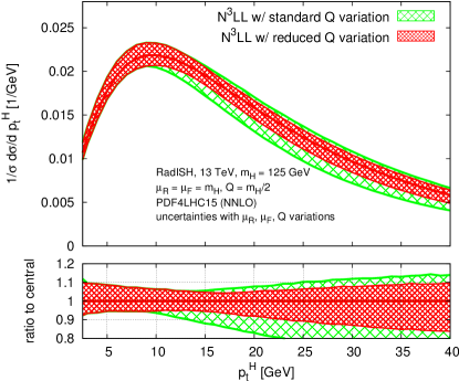
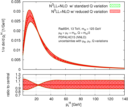
Figure 2: Comparison between two different prescriptions for the resummation-scale-variation range, as described in the text. The comparison is shown both at the resummation level (left) and with a matching to NLO (right).

We next turn to the comparison with NNLL. The left panel of Figure 3 shows a comparison between the pure resummed predictions for the normalised spectrum at N³LL and NNLL. In this plot, the NNLL curve is normalised to the NLO total cross section, while the N³LL curve is normalised to the NNLO total cross section. The plot shows that the inclusion of the N³LL corrections leads to a reduction in the scale uncertainty of the resummed prediction compared to the NNLL result.

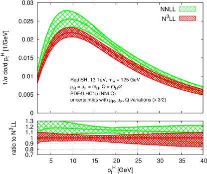
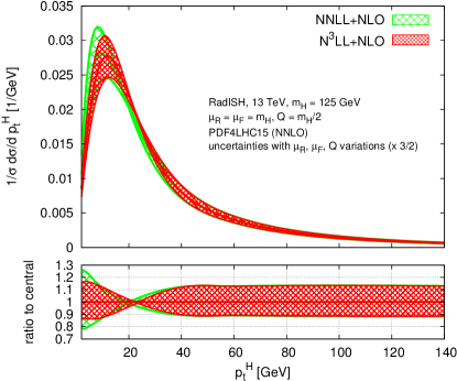
Figure 3: Left: comparison between the resummed distributions at N³LL and NNLL; the lower panel shows the ratio of the two distributions. Right: comparison between the matched N³LL+NLO and the NNLL+NLO predictions for the inclusive Higgs spectrum; the lower panel shows the ratio of each distribution to its central value.

The right plot of Figure 3 shows the matching of the NNLL and N³LL predictions to NLO. Both curves are now normalised to the NNLO total cross section. We observe that at the matched level, the N³LL corrections amount to $\sim 10\%$ around the peak of the spectrum, and they get slightly larger for smaller $p_{t}$ values ($\lesssim 10$ GeV). A substantial reduction of the total scale uncertainty is observed for $p_{t}\lesssim 10$ GeV.

We notice that, at the matched level, the impact of the N³LL corrections is reduced with respect to the sole resummation shown in the left plot of Figure 3. This is to a good extent due to the matching scheme that we chose here. Indeed, in a multiplicative scheme we include the ${\cal O}(\alpha_{s}^{2})$ constant terms already at NNLL, although they are formally of higher-order accuracy. While these terms enter at N³LL, they are numerically sizeable and therefore their inclusion reduces the difference between the N³LL+NLO and the NNLL+NLO predictions.

To conclude this section, in Figure 4 we report the N³LL+NNLO prediction for the normalised distribution. The latter is compared both to NNLL+NNLO and to the pure NNLO result. All curves in the plot are now normalised to the total N³LO cross section. When matched to NNLO, the N³LL corrections give rise to a few-percent shift of the central value with respect to the NNLL+NNLO prediction around the peak of the distributions, while they have a somewhat larger effect for $p_{t}\lesssim 10$ GeV. We recall that some of the N³LL effects are already included in the NNLL+NNLO prediction by means of the multiplicative matching scheme that we adopt here. As a consequence, this reduces the difference between the N³LL+NNLO and the NNLL+NNLO curves. We also observe that the matched N³LL and NNLL predictions are only moderately different in their theoretical-uncertainty bands. While this is of course expected in the hard region of the spectrum, we point out that, in the region $p_{t}\lesssim 30$ GeV, the latter feature is due (and increasingly so at smaller $p_{t}$) to numerical instabilities of the fixed-order runs with one of the scales ($\mu_{R}$ or $\mu_{F}$) set to $m_{H}/2$. As we already observed at NLO, it is indeed necessary to have stable fixed-order predictions for $p_{t}<10$ GeV in order to benefit from the uncertainty reduction due to the higher-order resummation. We leave this for future work.

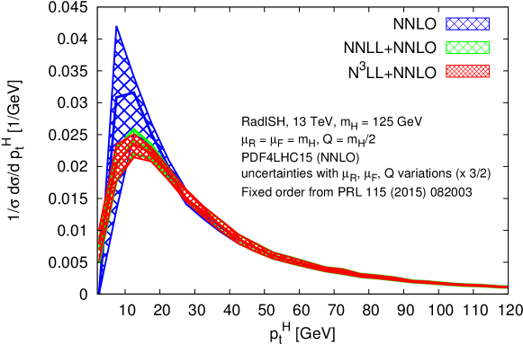
Figure 4: Comparison among the matched normalised distributions at N³LL+NNLO, NNLL+NNLO, and NNLO. The uncertainties are obtained as described in the text.

5 Conclusions

In this article we presented a formulation of the momentum-space resummation for global, recursive infrared and collinear safe observables that vanish far from the Sudakov limit because of kinematic cancellations implicit in the observable’s definition. In particular, we studied the class of inclusive observables that do not depend on the rapidity of the QCD radiation. Members of this class are, among others, the transverse momentum of a heavy colour singlet and the $\phi^{*}$ observable in Drell-Yan pair production. We obtained an all-order formula that is valid for all observables belonging to this class, and we explicitly evaluated it to N³LL up to effects due to the yet unknown four-loop cusp anomalous dimension. In the case of the transverse momentum of a colour singlet, we proved that our formulation is equivalent to the more common solution in impact-parameter space at this accuracy. This evidence is also supported by the numerous checks that we have documented. This equivalence allowed us to extract the ingredients necessary to compute the Sudakov radiator at N³LL using the recently computed $B^{(3)}$ coefficient Li:2016ctv ; Vladimirov:2016dll . The radiator is universal for all observables of this class Banfi:2014sua , which can therefore be resummed to this accuracy with our approach. The all-order result was shown to reproduce the correct power-like scaling in the small-$p_{t}$ limit, where the perturbative component of the coefficient of the intercept can be systematically improved by including higher-order logarithmic corrections. We implemented our results in the exclusive generator RadISH, which performs the resummation and the matching to fixed order, and allows the user to apply arbitrary kinematic cuts on the Born phase space. Although we explicitly treated the case of Higgs production, the code developed here can automatically handle any colour-singlet system.

As a phenomenological application, we computed the Higgs transverse-momentum spectrum at the LHC. In comparison to the NNLL+NLO prediction, we find that N³LL+NLO effects are moderate in size, and lead to ${\cal O}(10\%)$ corrections near the peak of the distribution and they are somewhat larger for $p_{t}\lesssim 10$ GeV. The scale uncertainty of the matched calculation is reduced by the inclusion of the N³LL corrections in the small transverse-momentum region. When matched to NNLO, the effect of the N³LL is pushed towards lower $p_{t}$ values, leading to a few percent correction to the previously known NNLL+NNLO prediction Monni:2016ktx around the peak, and to more sizeable effects at smaller $p_{t}$ values. In order to further improve the theoretical control in the small-medium transverse momentum region, it will be necessary to consider the deviations from the large-$m_{t}$ approximation. Recently, progress has been made in this respect by computing the NLO corrections to the top-bottom interference Lindert:2017pky . Higher-order effects due to the leading tower of logarithms of $p_{t}/m_{b}$ were addressed in ref. Melnikov:2016emg and were found to be moderate in size. The procedure for the inclusion of mass effects in the context of transverse-momentum resummation is a debated topic. While some prescriptions are available Grazzini:2013mca ; Banfi:2013eda , further studies are necessary to estimate these effects in the logarithmic region at this level of accuracy.

6 Acknowledgements

We wish to thank A. Banfi, C. Bauer, V. Bertone, G. Salam, G. Zanderighi for stimulating discussions on the topics treated here and very valuable comments on the manuscript. We also thank F. Caola for providing us with the fixed-order runs for the Higgs transverse-momentum spectrum at NNLO. The work of LR is supported by the European Research Council Starting Grant PDF4BSM, WB is supported by the European Research Council grant 614577 HICCUP (High Impact Cross Section Calculations for Ultimate Precision), and the work of ER is supported by a Marie Skłodowska-Curie Individual Fellowship of the European Commission’s Horizon 2020 Programme under contract number 659147 PrecisionTools4LHC. PM would like to thank the Erwin Schrödinger Institute of Vienna for hospitality and support while part of this work was carried out. PT would like to thank CERN’s Thoretical Physics Department for hospitality during the development of this work.

Appendix A Connection with the backward-evolution algorithm at NLL

It is interesting to relate our formulation for the transverse-momentum resummation to a NLL-accurate backward-evolution algorithm Sjostrand:1985xi ; Gottschalk:1986bk ; Marchesini:1987cf . We start from Eq. (2.3.3), that was deduced by considering only flavour-conserving real splitting kernels, for the sake of clarity. We briefly comment on the general flavour case below.

After neglecting the effect of the hard and coefficient functions, which starts at NNLL, we recast the NLL partonic cross section as

$$\hat{\bf\Sigma}_{N_{1},N_{2}}^{c_{1},c_{2}}(v)=\mathbb{1}^{(c_{1},c_{2})}\int_{0}^{M}\frac{dk_{t1}}{k_{t1}}\int_{0}^{2\pi}\frac{d\phi_{1}}{2\pi}e^{-{\bf R}(\epsilon k_{t1})}\exp\left\{-\sum_{\ell=1}^{2}\int_{\epsilon k_{t1}}^{\mu_{0}}\frac{dk_{t}}{k_{t}}\frac{\alpha_{s}(k_{t})}{\pi}{\bf\Gamma}_{N_{\ell}}(\alpha_{s}(k_{t}))\right\}$$

$$\sum_{\ell_{1}=1}^{2}\left({\bf R}_{\ell_{1}}^{\prime}\left(k_{t1}\right)+\frac{\alpha_{s}(k_{t1})}{\pi}{\bf\Gamma}_{N_{\ell_{1}}}(\alpha_{s}(k_{t1}))\right)\sum_{n=0}^{\infty}\frac{1}{n!}\prod_{i=2}^{n+1}\int_{\epsilon}^{1}\frac{d\zeta_{i}}{\zeta_{i}}\int_{0}^{2\pi}\frac{d\phi_{i}}{2\pi}$$

$$\times\sum_{\ell_{i}=1}^{2}\bigg{(}{\bf R}_{\ell_{i}}^{\prime}\left(k_{ti}\right)+\frac{\alpha_{s}(k_{ti})}{\pi}{\bf\Gamma}_{N_{\ell_{i}}}(\alpha_{s}(k_{ti}))\bigg{)}\Theta\left(v-V(\{\tilde{p}\},k_{1},\dots,k_{n+1})\right),$$ (143)

where $\mathbb{1}^{(c_{1},c_{2})}$ enforces the flavour of the two parton densities to be identical to that entering the Born process, i.e. ${\bf f}^{T}\mathbb{1}^{(c_{1},c_{2})}{\bf f}=f_{c_{1}}f_{c_{2}}$. At NLL order, the emission probabilities involve only tree-level splitting functions, whose coupling we evaluate in the CMW scheme, as discussed in Sec. 2.1:

$$\frac{\alpha_{s}(k_{t})}{\pi}\to\frac{\alpha^{\rm CMW}_{s}(k_{t})}{\pi}=\frac{\alpha_{s}(k_{t})}{\pi}\left(1+\frac{\alpha_{s}(k_{t})}{2\pi}K\right),$$ (144)

where $K$ is defined in Eq. (22). In order to perform the inverse Mellin transform of Eq. (A), we observe that, when inverted into $z$ space, each of the real-emission probabilities acts on a generic parton distribution $f(x_{\ell_{i}})$ as described in Section 2.3.3:

$$\bigg{(}R_{\ell_{i}}^{\prime}\left(k_{ti}\right) +\frac{\alpha_{s}(k_{ti})}{\pi}\gamma^{(0)}_{N_{\ell_{i}}}(\alpha_{s}(k_{ti}))\bigg{)}f_{N_{\ell_{i}}}(\mu)$$

$$\to\frac{\alpha^{\rm CMW}_{s}(k_{ti})}{\pi}\Bigg{(}\int_{0}^{1-k_{ti}/M}dz_{i}^{(\ell_{i})}P^{(0)}(z_{i}^{(\ell_{i})})f(\mu,x_{\ell_{i}})+\int_{x_{\ell_{i}}}^{1}dz_{i}^{(\ell_{i})}\frac{\hat{P}^{(0)}(z_{i}^{(\ell_{i})})}{z_{i}^{(\ell_{i})}}f(\mu,\frac{x_{\ell_{i}}}{z_{i}^{(\ell_{i})}})\Bigg{)},$$ (145)

where we reintroduced the regular terms in the hard-collinear contribution to $R^{\prime}_{\ell}$, whose $z^{(\ell)}$ upper limit was set to $1$ in Section 2.3.2.

Similarly, we can now restore the remaining power-suppressed terms in the single-emission probability that we neglected in our discussion of Section 2.3.2, and recast the right-hand side of Eq. (A) in terms of the unregularised splitting function as

$$\frac{\alpha_{s}^{\rm CMW}(k_{ti})}{\pi}\int_{x_{\ell_{i}}}^{1-k_{ti}/M}dz_{i}^{(\ell_{i})}\frac{P^{(0)}(z_{i}^{(\ell_{i})})}{z_{i}^{(\ell_{i})}}f(\mu,\frac{x_{\ell_{i}}}{z_{i}^{(\ell_{i})}}).$$ (146)

We furthermore introduce the shower Sudakov form factor $\Delta(Q_{i})$, that at NLL reads

$$\Delta(Q_{i})=\exp\left\{-\sum_{\ell=1}^{2}\int^{Q_{i}}_{\epsilon k_{t1}}\frac{dk_{t}}{k_{t}}\int_{0}^{1-k_{t}/M}dz^{(\ell)}\frac{\alpha^{\rm CMW}_{s}(k_{t})}{\pi}P^{(0)}(z^{(\ell)})\right\},$$ (147)

such that $\Delta(M)=\exp\left\{-R_{\rm NLL}(\epsilon k_{t1})\right\}$ up to non-logarithmic terms included in $\Delta$ but not in $\exp\left\{-R\right\}$.

As shown in the main text, in the all-order picture, the correct $z^{(\ell)}$ bounds for each emission depend on the radiation that was emitted before it. Following the discussion of Section 2.1, however, we recall that these effects contribute beyond NLL accuracy, and therefore can be neglected in the present case. We then plug Eq. (A) into Eq. (62) and perform the inverse Mellin transform as just described, obtaining

$$\frac{d\Sigma(v)}{d\Phi_{B}}=\frac{d|M_{B}|_{c_{1}c_{2}}^{2}}{d\Phi_{B}}$$

$$\times\int_{0}^{M}\frac{dk_{t1}}{k_{t1}}\int_{0}^{2\pi}\frac{d\phi_{1}}{2\pi}\frac{\Delta(M)}{\Delta(k_{t1})}\sum_{\ell_{1}=1}^{2}\int_{x_{\ell_{1}}}^{1-k_{t1}/M}dz_{1}^{(\ell_{1})}\frac{\alpha^{\rm CMW}_{s}(k_{t1})}{\pi}\frac{P^{(0)}(z_{1}^{(\ell_{1})})}{z_{1}^{(\ell_{1})}}\sum_{n=0}^{\infty}\frac{1}{n!}\prod_{i=2}^{n+1}\int_{\epsilon}^{1}\frac{d\zeta_{i}}{\zeta_{i}}\int_{0}^{2\pi}\frac{d\phi_{i}}{2\pi}$$

$$\times\frac{\Delta(k_{t(i-1)})}{\Delta(k_{ti})}\sum_{\ell_{i}=1}^{2}\int_{w_{\ell_{i}}}^{1-\zeta_{i}k_{t1}/M}dz_{i}^{(\ell_{i})}\frac{\alpha^{\rm CMW}_{s}(k_{ti})}{\pi}\frac{P^{(0)}(z_{i}^{(\ell_{i})})}{z_{i}^{(\ell_{i})}}f_{c_{1}}(\epsilon k_{t1},\bar{x}_{1})f_{c_{2}}(\epsilon k_{t1},\bar{x}_{2})$$

$$\hskip 256.0748pt\times\Theta\left(v-V(\{\tilde{p}\},k_{1},\dots,k_{n+1})\right),$$ (148)

with $\Delta(\epsilon k_{t1})=1$ and

$$w_{\ell_{i}}=x_{\ell_{i}}/\left(\prod_{\begin{subarray}{c}j=1\\ \ell_{j}=\ell_{i}\end{subarray}}^{i-1}z_{j}^{(\ell_{j})}\right),\qquad\bar{x}_{1}=x_{1}/\left(\prod_{\begin{subarray}{c}j=1\\ \ell_{j}=1\end{subarray}}^{n+1}z_{j}^{(\ell_{j})}\right),\qquad\bar{x}_{2}=x_{2}/\left(\prod_{\begin{subarray}{c}j=1\\ \ell_{j}=2\end{subarray}}^{n+1}z_{j}^{(\ell_{j})}\right).$$ (149)

We stress again that the $z_{i}^{(\ell)}$ limits in Eq. (A) are obtained in the approximation of soft kinematics which is valid at NLL accuracy. To implement Eq. (A) in a Markov process we can now impose an ordering in the transverse momentum of the emissions, which amounts to performing the following replacement in Eq. (A) (we remind that $\zeta_{i}=k_{ti}/k_{t1}$)

$$\frac{1}{n!}\prod_{i=2}^{n+1}\int_{\epsilon}^{1}\frac{d\zeta_{i}}{\zeta_{i}}\to\int_{\epsilon}^{1}\frac{d\zeta_{2}}{\zeta_{2}}\int_{\epsilon}^{\zeta_{2}}\frac{d\zeta_{3}}{\zeta_{3}}\dots\int_{\epsilon}^{\zeta_{n}}\frac{d\zeta_{n+1}}{\zeta_{n+1}}.$$ (150)

With this replacement, Eq. (A) reproduces the backward-evolution equation for a shower of primary gluons emitted off the two initial-state legs (see e.g. Eq. (49) of ref. Marchesini:1987cf ), ordered in transverse momentum. The only relevant difference with the common parton-shower formulation is in the fact that, unlike a parton shower, Eq. (A) does not contain a no-emission event. This term is indeed infinitely suppressed in our case and therefore it does not contribute to the final result. As a consequence, the cutoff (represented by $\epsilon k_{t1}$ in our formula) is replaced by a fixed cut $Q_{0}$ in the trasverse momentum of the emissions. In order for Eq. (A) to be NLL accurate for the transverse-momentum distribution, the recoil of all initial-state emissions must be entirely absorbed by the colour singlet. This shows that a branching algorithm for initial-state radiation that fulfils the above conditions is NLL accurate for this observable (see also Catani:1990rr ). Analogous considerations apply to other rIRC safe, global observables of the type (6). To extend the above discussion to the generic flavour case, one is forced to relax the assumption of $k_{t}$ ordering in order to implement the above solution in a Markov-chain Monte-Carlo program. Indeed, if some soft radiation occurs after the flavour-changing collinear emission has taken place, then it becomes quite cumbersome to determine the correct colour factor for the former. This is because coherence guarantees that a soft gluon feels the effective colour charge of the radiation at smaller angles, which now may involve combinations of different flavours. A correct solution to this problem requires to reformulate the evolution by ordering the radiation in angle. This ensures that the hard-collinear emissions contributing to the DGLAP evolution happen at last (see also the discussion in Appendix E.2 of ref. Banfi:2004yd ), and the colour structure of the soft radiation is easily determined. It is possible to show that the backward-evolution algorithm reproduces the resulting evolution formula in that case as well, and it is therefore NLL accurate.

Appendix B Analytic formulae for the N³LL radiator

In this Appendix we report the expressions for some of the quantities used in the article. The RGE equation for the QCD coupling reads

$$\frac{d\alpha_{s}(\mu)}{d\ln\mu^{2}}=\beta(\alpha_{s})\equiv-\alpha_{s}\left(\beta_{0}\alpha_{s}+\beta_{1}\alpha_{s}^{2}+\beta_{2}\alpha_{s}^{3}+\beta_{3}\alpha_{s}^{4}+\dots\right).$$ (151)

The coefficients of the $\beta$ function (with $n_{f}$ active flavours) are

$$\beta_{0}=\frac{11C_{A}-2n_{f}}{12\pi}\,,\quad\beta_{1}=\frac{17C_{A}^{2}-5C_{A}n_{f}-3C_{F}n_{f}}{24\pi^{2}}\,,$$ (152)

$$\beta_{2} = \frac{2857C_{A}^{3}+(54C_{F}^{2}-615C_{F}C_{A}-1415C_{A}^{2})n_{f}+(66C_{F}+79C_{A})n_{f}^{2}}{3456\pi^{3}}\,,$$ (153)

$$\beta_{3} = \frac{1}{(4\pi)^{4}}\Bigg{\{}C_{A}C_{F}n_{f}^{2}\frac{1}{4}\left(\frac{17152}{243}+\frac{448}{9}\zeta_{3}\right)+C_{A}C_{F}^{2}n_{f}\frac{1}{2}\left(-\frac{4204}{27}+\frac{352}{9}\zeta_{3}\right)$$ (154)

$$\hskip 28.45274pt+\frac{53}{243}C_{A}n_{f}^{3}+C_{A}^{2}C_{F}n_{f}\frac{1}{2}\left(\frac{7073}{243}-\frac{656}{9}\zeta_{3}\right)+C_{A}^{2}n_{f}^{2}\frac{1}{4}\left(\frac{7930}{81}+\frac{224}{9}\zeta_{3}\right)$$

$$\hskip 28.45274pt+\frac{154}{243}C_{F}n_{f}^{3}+C_{A}^{3}n_{f}\frac{1}{2}\left(-\frac{39143}{81}+\frac{136}{3}\zeta_{3}\right)+C_{A}^{4}\left(\frac{150653}{486}-\frac{44}{9}\zeta_{3}\right)$$

$$\hskip 28.45274pt+C_{F}^{2}n_{f}^{2}\frac{1}{4}\left(\frac{1352}{27}-\frac{704}{9}\zeta_{3}\right)+23C_{F}^{3}n_{f}+n_{f}\frac{d_{F}^{abcd}d_{A}^{abcd}}{N_{A}}\left(\frac{512}{9}-\frac{1664}{3}\zeta_{3}\right)$$

$$\hskip 28.45274pt+n_{f}^{2}\frac{d_{F}^{abcd}d_{F}^{abcd}}{N_{A}}\left(-\frac{704}{9}+\frac{512}{3}\zeta_{3}\right)+\frac{d_{A}^{abcd}d_{A}^{abcd}}{N_{A}}\left(-\frac{80}{9}+\frac{704}{3}\zeta_{3}\right)\Bigg{\}}\,,$$

where

$$\frac{d_{F}^{abcd}d_{F}^{abcd}}{N_{A}} = \frac{N_{c}^{4}-6N_{c}^{2}+18}{96N_{c}^{2}},$$

$$\frac{d_{F}^{abcd}d_{A}^{abcd}}{N_{A}} = \frac{N_{c}(N_{c}^{2}+6)}{48},$$

$$\frac{d_{A}^{abcd}d_{A}^{abcd}}{N_{A}} = \frac{N_{c}^{2}(N_{c}^{2}+36)}{24},$$

and $C_{A}=N_{c}$, $C_{F}=\frac{N_{c}^{2}-1}{2N_{c}}$, and $N_{c}=3$.

The lowest-order regularised Altarelli-Parisi splitting functions in four dimensions are

$$\hat{P}^{(0)}_{qq}(z) = C_{F}\left[\frac{1+z^{2}}{(1-z)_{+}}+\frac{3}{2}\delta(1-z)\right],$$

$$\hat{P}^{(0)}_{qg}(z) = \frac{1}{2}\left[z^{2}+(1-z)^{2}\right],$$

$$\hat{P}^{(0)}_{gq}(z) = C_{F}\frac{1+(1-z)^{2}}{z},$$

$$\hat{P}^{(0)}_{gg}(z) = 2C_{A}\left[\frac{z}{(1-z)_{+}}+\frac{1-z}{z}+z(1-z)\right]+2\pi\beta_{0}\delta(1-z),$$ (155)

where the plus prescription is defined as

$$\int_{0}^{1}dz\,\frac{f(z)}{(1-z)_{+}}=\int_{0}^{1}dz\,\frac{f(z)-f(1)}{1-z}.$$ (156)

The corresponding unregularised Altarelli-Parisi splitting functions in four dimensions are

$$P^{(0)}_{qq}(z) = C_{F}\frac{1+z^{2}}{1-z},$$

$$P^{(0)}_{qg}(z) = \frac{1}{2}\left[z^{2}+(1-z)^{2}\right],$$

$$P^{(0)}_{gq}(z) = C_{F}\frac{1+(1-z)^{2}}{z},$$

$$P^{(0)}_{gg}(z) = C_{A}\left[\frac{z}{1-z}+\frac{1-z}{z}+z(1-z)\right]\rightarrow C_{A}\left[2\frac{z}{1-z}+z(1-z)\right],$$ (157)

where in the last step we exploited the symmetry of the $P^{(0)}_{gg}(z)$ splitting function in $z\rightarrow 1-z$.

Next we report the functions that enter the definition of the Sudakov radiator (Eq. (4.1)) up to NNLL. To simplify the notation we set $\lambda=\alpha_{s}(\mu_{R})\beta_{0}L$. They read

$$g_{1}(\alpha_{s}L)= \frac{A^{(1)}}{\pi\beta_{0}}\frac{2\lambda+\ln(1-2\lambda)}{2\lambda},$$ (158)

$$g_{2}(\alpha_{s}L)= \frac{1}{2\pi\beta_{0}}\ln(1-2\lambda)\left(A^{(1)}\ln\frac{1}{x_{Q}^{2}}+B^{(1)}\right)-\frac{A^{(2)}}{4\pi^{2}\beta_{0}^{2}}\frac{2\lambda+(1-2\lambda)\ln(1-2\lambda)}{1-2\lambda}$$

$$+A^{(1)}\bigg{(}-\frac{\beta_{1}}{4\pi\beta_{0}^{3}}\frac{\ln(1-2\lambda)((2\lambda-1)\ln(1-2\lambda)-2)-4\lambda}{1-2\lambda}$$

$$\hskip 28.45274pt-\frac{1}{2\pi\beta_{0}}\frac{(2\lambda(1-\ln(1-2\lambda))+\ln(1-2\lambda))}{1-2\lambda}\ln\frac{\mu_{R}^{2}}{x_{Q}^{2}M^{2}}\bigg{)}\,,$$ (159)

$$g_{3}(\alpha_{s}L)= \left(A^{(1)}\ln\frac{1}{x_{Q}^{2}}+B^{(1)}\right)\bigg{(}-\frac{\lambda}{1-2\lambda}\ln\frac{\mu_{R}^{2}}{x_{Q}^{2}M^{2}}+\frac{\beta_{1}}{2\beta_{0}^{2}}\frac{2\lambda+\ln(1-2\lambda)}{1-2\lambda}\bigg{)}$$

$$-\frac{1}{2\pi\beta_{0}}\frac{\lambda}{1-2\lambda}\left(A^{(2)}\ln\frac{1}{x_{Q}^{2}}+B^{(2)}\right)-\frac{A^{(3)}}{4\pi^{2}\beta_{0}^{2}}\frac{\lambda^{2}}{(1-2\lambda)^{2}}$$

$$+A^{(2)}\bigg{(}\frac{\beta_{1}}{4\pi\beta_{0}^{3}}\frac{2\lambda(3\lambda-1)+(4\lambda-1)\ln(1-2\lambda)}{(1-2\lambda)^{2}}-\frac{1}{\pi\beta_{0}}\frac{\lambda^{2}}{(1-2\lambda)^{2}}\ln\frac{\mu_{R}^{2}}{x_{Q}^{2}M^{2}}\bigg{)}$$

$$+A^{(1)}\bigg{(}\frac{\lambda\left(\beta_{0}\beta_{2}(1-3\lambda)+\beta_{1}^{2}\lambda\right)}{\beta_{0}^{4}(1-2\lambda)^{2}}+\frac{(1-2\lambda)\ln(1-2\lambda)\left(\beta_{0}\beta_{2}(1-2\lambda)+2\beta_{1}^{2}\lambda\right)}{2\beta_{0}^{4}(1-2\lambda)^{2}}$$

$$\hskip 28.45274pt+\frac{\beta_{1}^{2}}{4\beta_{0}^{4}}\frac{(1-4\lambda)\ln^{2}(1-2\lambda)}{(1-2\lambda)^{2}}-\frac{\lambda^{2}}{(1-2\lambda)^{2}}\ln^{2}\frac{\mu_{R}^{2}}{x_{Q}^{2}M^{2}}$$

$$\hskip 28.45274pt-\frac{\beta_{1}}{2\beta_{0}^{2}}\frac{(2\lambda(1-2\lambda)+(1-4\lambda)\ln(1-2\lambda))}{(1-2\lambda)^{2}}\ln\frac{\mu_{R}^{2}}{x_{Q}^{2}M^{2}}\bigg{)}.$$ (160)

The new N³LL $g_{4}$ coefficient reads

$$g_{4}(\alpha_{s}L) = \frac{A^{(4)}(3-2\lambda)\lambda^{2}}{24\pi^{2}\beta_{0}^{2}(2\lambda-1)^{3}}$$ (161)

$$+\frac{A^{(3)}}{48\pi\beta_{0}^{3}(2\lambda-1)^{3}}\Bigg{\{}3\beta_{1}(1-6\lambda)\ln(1-2\lambda)+2\lambda\Bigg{(}\beta_{1}(5\lambda(2\lambda-3)+3)$$

$$\hskip 28.45274pt+6\beta_{0}^{2}(3-2\lambda)\lambda\ln\frac{\mu_{R}^{2}}{x_{Q}^{2}M^{2}}\Bigg{)}+12\beta_{0}^{2}(\lambda-1)\lambda(2\lambda-1)\ln\frac{1}{x_{Q}^{2}}\Bigg{\}}$$

$$+\frac{A^{(2)}}{24\beta_{0}^{4}(2\lambda-1)^{3}}\Bigg{\{}32\beta_{0}\beta_{2}\lambda^{3}-2\beta_{1}^{2}\lambda(\lambda(22\lambda-9)+3)$$

$$\hskip 28.45274pt+12\beta_{0}^{4}(3-2\lambda)\lambda^{2}\ln^{2}\frac{\mu_{R}^{2}}{x_{Q}^{2}M^{2}}+6\beta_{0}^{2}\ln\frac{\mu_{R}^{2}}{x_{Q}^{2}M^{2}}\times$$

$$\hskip 28.45274pt\left(\beta_{1}(1-6\lambda)\ln(1-2\lambda)+2(\lambda-1)\lambda(2\lambda-1)\left(\beta_{1}+2\beta_{0}^{2}\ln\frac{1}{x_{Q}^{2}}\right)\right)$$

$$\hskip 28.45274pt+3\beta_{1}\Bigg{(}\beta_{1}\ln(1-2\lambda)(2\lambda+(6\lambda-1)\ln(1-2\lambda)-1)$$

$$\hskip 28.45274pt-2\beta_{0}^{2}(2\lambda-1)(2(\lambda-1)\lambda-\ln(1-2\lambda))\ln\frac{1}{x_{Q}^{2}}\Bigg{)}\Bigg{\}}$$

$$+\frac{\pi A^{(1)}}{12\beta_{0}^{5}(2\lambda-1)^{3}}\Bigg{\{}\beta_{1}^{3}(1-6\lambda)\ln^{3}(1-2\lambda)+3\ln(1-2\lambda)\Bigg{(}\beta_{0}^{2}\beta_{3}(2\lambda-1)^{3}$$

$$\hskip 28.45274pt+\beta_{0}\beta_{1}\beta_{2}\left(1-2\lambda\left(8\lambda^{2}-4\lambda+3\right)\right)+4\beta_{1}^{3}\lambda^{2}(2\lambda+1)$$

$$\hskip 28.45274pt+\beta_{0}^{2}\beta_{1}\ln\frac{\mu_{R}^{2}}{x_{Q}^{2}M^{2}}\left(\beta_{0}^{2}(1-6\lambda)\ln\frac{\mu_{R}^{2}}{x_{Q}^{2}M^{2}}-4\beta_{1}\lambda\right)\Bigg{)}$$

$$\hskip 28.45274pt+3\beta_{1}^{2}\ln^{2}(1-2\lambda)\left(2\beta_{1}\lambda+\beta_{0}^{2}(6\lambda-1)\ln\frac{\mu_{R}^{2}}{x_{Q}^{2}M^{2}}\right)$$

$$\hskip 28.45274pt+3\beta_{0}^{2}(2\lambda-1)\ln\frac{1}{x_{Q}^{2}}\Bigg{(}-\beta_{1}^{2}\ln^{2}(1-2\lambda)+2\beta_{0}^{2}\beta_{1}\ln(1-2\lambda)\ln\frac{\mu_{R}^{2}}{x_{Q}^{2}M^{2}}$$

$$\hskip 28.45274pt+4\lambda\left(\lambda\left(\beta_{1}^{2}-\beta_{0}\beta_{2}\right)+\beta_{0}^{4}(\lambda-1)\ln^{2}\frac{\mu_{R}^{2}}{x_{Q}^{2}M^{2}}\right)\Bigg{)}$$

$$\hskip 28.45274pt+2\lambda\Bigg{(}\beta_{0}^{2}\beta_{3}((15-14\lambda)\lambda-3)+\beta_{0}\beta_{1}\beta_{2}(5\lambda(2\lambda-3)+3)$$

$$\hskip 28.45274pt+4\beta_{1}^{3}\lambda^{2}+2\beta_{0}^{6}(3-2\lambda)\lambda\ln^{3}\frac{\mu_{R}^{2}}{x_{Q}^{2}M^{2}}+3\beta_{0}^{4}\beta_{1}\ln^{2}\frac{\mu_{R}^{2}}{x_{Q}^{2}M^{2}}$$

$$\hskip 28.45274pt+6\beta_{0}^{2}\lambda(2\lambda+1)\left(\beta_{0}\beta_{2}-\beta_{1}^{2}\right)\ln\frac{\mu_{R}^{2}}{x_{Q}^{2}M^{2}}-8\beta_{0}^{6}\left(4\lambda^{2}-6\lambda+3\right)\zeta_{3}\Bigg{)}\Bigg{\}}$$

$$+\frac{B^{(3)}(\lambda-1)\lambda}{4\pi\beta_{0}(1-2\lambda)^{2}}+\frac{B^{(2)}\left(\beta_{1}\ln(1-2\lambda)-2(\lambda-1)\lambda\left(\beta_{1}-2\beta_{0}^{2}\ln\frac{\mu_{R}^{2}}{x_{Q}^{2}M^{2}}\right)\right)}{4\beta_{0}^{2}(1-2\lambda)^{2}}$$

$$+\frac{\pi B^{(1)}}{4\beta_{0}^{3}(1-2\lambda)^{2}}\Bigg{\{}4\lambda\left(\lambda\left(\beta_{1}^{2}-\beta_{0}\beta_{2}\right)+\beta_{0}^{4}(\lambda-1)\ln^{2}\frac{\mu_{R}^{2}}{x_{Q}^{2}M^{2}}\right)$$

$$\hskip 28.45274pt-\beta_{1}^{2}\ln^{2}(1-2\lambda)+2\beta_{0}^{2}\beta_{1}\ln(1-2\lambda)\ln\frac{\mu_{R}^{2}}{x_{Q}^{2}M^{2}}\Bigg{\}}.$$

Appendix C Additional considerations on the small-$p_{t}$ scaling

In this Appendix we discuss further the analysis of the $p_{t}\to 0$ limit of the differential cross section carried out in Sec. 3.2. Specifically, following Ref. Parisi:1979se , we have made a number of approximations to derive the scaling of the integral (3.2) with $\Lambda^{2}_{\rm QCD}/M^{2}$. Such approximations, however, are too rough to capture the correct ${\cal O}(1)$ normalisation of the scaling, and in this appendix we quantify the difference from the correct result obtained by directly integrating Eq. (3.2).

For the sake of convenience, we define the quantity

$$\Delta\equiv\lim_{p_{t}\rightarrow 0}\frac{1}{\sigma^{(0)}(\Phi_{B})}\frac{d^{2}\Sigma(v)}{p_{t}dp_{t}d\Phi_{B}}\equiv\lim_{p_{t}\rightarrow 0}\frac{d\bar{\sigma}}{p_{t}dp_{t}}\,,$$ (162)

where $\frac{d^{2}\Sigma(v)}{p_{t}dp_{t}d\Phi_{B}}$ was obtained in Eq. (3.2). The $p_{t}\to 0$ limit simply corresponds to setting $J_{0}(p_{t}b)=1+\mathcal{O}(p_{t}^{2})$, leading to

$$\Delta =\int\!\!b\,db\int\frac{dk_{t1}}{k_{t1}}e^{-R(k_{t1})}R^{\prime}(k_{t1})J_{0}(bk_{t1})$$

$$\hskip 113.81102pt\times\exp\left\{-R^{\prime}\left(k_{t1}\right)\int^{k_{t1}}_{0}\frac{dk_{t}}{k_{t}}(1-J_{0}(bk_{t}))\right\}.$$ (163)

The result given in Eq. (118) and (119) has been obtained by further approximating the integral in Eq. (117) with its asymptotic behaviour. While this approximation is sufficient to capture the correct scaling of the cross section at $p_{t}=0$, it leads to an inaccurate estimate of the ${\cal O}(1)$ normalisation. For comparison, we then recall Eq. (118):

$$\Delta_{\textrm{approx.}}=4\int\frac{dk_{t1}}{k_{t1}^{3}}e^{-R(k_{t1})}\,.$$ (164)

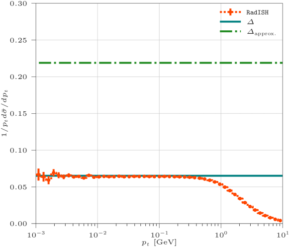
Figure 5: Comparison of different approximations for the small-$p_{t}$ limit.

To numerically quantify the difference between Eqs. (164) and (C), we consider the case of $Z$ production with $m_{Z}=91.1876$ GeV. We evaluate numerically Eq. (C) and Eq. (164) and we compare them with the prediction obtained with the RadISH code. For the sake of simplicity, we use everywhere the LL expressions for $R$ and its derivative $R^{\prime}$. To regulate the $b\rightarrow 0$ ($+\infty$) limits in Eq. (C) we set a lower (upper) limit of $b_{0}/m_{Z}$ ($b_{0}/Q_{0}$) in the $b$ integral, where $Q_{0}$ is the Landau singularity of the integrand which reads

$$Q_{0}=m_{Z}\,e^{-\frac{1}{2\alpha_{s}\beta_{0}}}\,.$$ (165)

Correspondingly, we integrate over $k_{t1}$ in both Eqs. (C) and (164) between $Q_{0}$ and $m_{Z}$ and we use the same limits in the numerical results obtained with RadISH. The results are displayed in Fig. 5, where we observe that the numerical result obtained with RadISH converges in the $p_{t}\rightarrow 0$ limit to the result given in Eq. (C). Both results differ significantly from the approximated result Eq. (164), which overestimates the normalisation by more than a factor of three. We observe that such a difference can be also obtained by computing the ratio of Eq. (164) to the $p_{t}\to 0$ limit of the original $b$-space formulation.