Configuration spaces of spatial linkages: Taking Collisions Into Account

Abstract.

We construct a completed version  $\widehat{{\mathcal{C}}}(\Gamma)$   of the configuration space of a linkage $\Gamma$ in  ${\mathbb{R}}^{3}$,  which takes into account the ways one link can touch another. We also describe a simplified version  $\underline{{\mathcal{C}}}(\Gamma)$   which is a blow-up of the space of immersions of $\Gamma$ in  ${\mathbb{R}}^{3}$.  A number of simple detailed examples are given.

0. Introduction

A linkage is a collection of rigid bars, or links, attached to each other at their vertices, with a variety of possible joints (fixed, spherical, rotational, and so on). These play a central role in the field of robotics, in both its mathematical and engineering aspects: see [Me, Se, T, Fa].

Such a linkage $\Gamma$, thought of as a metric graph, can be embedded in an ambient Euclidean space  ${\mathbb{R}}^{d}$   in various ways, called configurations of $\Gamma$. The space  ${\mathcal{C}}({\Gamma})$   of all such configurations has a natural topology and differentiable structure  –  see [Hal] and Section 1 below.

Such configuration spaces have been studied extensively, mostly for simple closed or open chains (cf. [FTY, G, HK, JS, KM1, MT]; but see [Ho, KT, OH, SSB]). In the plane, the convention is that links freely slide over each other, so that a configuration is determined solely by the locations of the joints. This convention is usually extended to spaces of polygons in  ${\mathbb{R}}^{3}$   (see, e.g., [KM2]), so they no longer provide realistic models of linkages (since in this model the links can pass through each other freely). Alternatively, some authors have studies spaces of embeddings of sets of disjoint lines in  ${\mathbb{R}}^{3}$,  for which the issue does not arise (cf. [CEGSS, DV, Vi]).

The goal of this paper is to address this question for spatial linkages, by constructing a model taking into account how different bars touch each other. We still use a simplified mathematical model, in which the links have no thickness, and so on. Our starting point is the space  ${\mathcal{C}}({\Gamma})$   of embeddings of $\Gamma$ in  ${\mathbb{R}}^{3}$.  If we allow the links to intersect, we obtain the larger space  ${\mathcal{C}}\,^{\operatorname{im}}(\Gamma)$   of immersions of $\Gamma$ in  ${\mathbb{R}}^{3}$.  However,  ${\mathcal{C}}\,^{\operatorname{im}}(\Gamma)$   disregards the fact that in reality two bars touch each other on one side or the other. To take this into account, we construct the completed configuration space  $\widehat{{\mathcal{C}}}(\Gamma)$   from  ${\mathcal{C}}({\Gamma})$   by completing it with respect to a suitable metric. The new points of  $\widehat{{\mathcal{C}}}(\Gamma)\setminus{\mathcal{C}}({\Gamma})$   are called virtual configurations: they correspond to immersed configurations decorated with an additional (discrete) set of labels. See Section 2.

Unfortunately, the completed configuration space  $\widehat{{\mathcal{C}}}(\Gamma)$   is very difficult to describe in most cases. Therefore, we also construct a simplified version, called the blow-up, denoted by  $\underline{{\mathcal{C}}}(\Gamma)$.  Here the labelling is described explicitly by a finite set of invariants (see Proposition 3.6 below), called linking numbers, which determine the mutual position of two infinitely thin tangent cylinders in space (cf. [Va]). See Section 3.

One advantage of the blow-up is that its set of singularities can be filtered in various ways, and the simpler types can be described explicitly. See Section 4.

The relation between these spaces can be described as follows:

(0.1)

The second half of the paper is devoted to the study of a number of examples:

1. The simplest “linkage” we describe consists of two oriented lines in  ${\mathbb{R}}^{3}$.  In this case  $\widehat{{\mathcal{C}}}(\Gamma)=\underline{{\mathcal{C}}}(\Gamma)$,  and the configuration space is described fully in §5.A.

2. More generally, in Section 6 we consider a collection of $n$ oriented lines in space, and show that its completed configuration space is homotopy equivalent to that of a linkage consisting of $n$ lines touching at the origin.

   We give a full cell structure for  $\widehat{{\mathcal{C}}}(\Gamma)$   when  $n=3$   in Section 7.

3. Finally, the case of a closed quadrilateral chain is analyzed in §8.A and that of an open chain of length three in §8.B.

1. Configuration spaces

Any embedding of a linkage in a (fixed) ambient Euclidean space  ${\mathbb{R}}^{d}$   is determined by the positions of its vertices, but not all embeddings of its vertices determine a legal embedding of the linkage. To make this precise, we require the following:

1.1 Definition.

An linkage type is a graph  ${\mathcal{T}}_{\Gamma}=(V,E)$,  determined by a set $V$ of $N$ vertices and a set  $E\subseteq V^{2}$   of $k$ edges (between distinct vertices). We assume there are no isolated vertices. A specific linkage  $\Gamma=({\mathcal{T}}_{\Gamma},\vec{\ell})$   of type  ${\mathcal{T}}_{\Gamma}$   is determined by a length vector  $\vec{\ell}:=(\ell_{1},\dotsc,\ell_{k})\in{\mathbb{R}}^{E}_{+}$,  specifying the length  $\ell_{i}>0$   of each edge  $(u_{i},v_{i})$   in $E$  ($i=1,\dotsc,k$).  This  $\vec{\ell}$   is required to satisfy the triangle inequality where appropriate. We call an edge with a specified length a link, (or bar) of the linkage $\Gamma$, and the vertices of $\Gamma$ are also known as joints.

An embedding of  ${\mathcal{T}}_{\Gamma}$   in the Euclidean space  ${\mathbb{R}}^{d}$   is an injective map  $\mathbf{x}:V\to{\mathbb{R}}^{d}$   such that the open intervals  $(\mathbf{x}(u_{i}),\mathbf{x}(v_{i}))$   and  $(\mathbf{x}(u_{j}),\mathbf{x}(v_{j}))$   in  ${\mathbb{R}}^{d}$   are disjoint if the edges  $(u_{i},v_{i})$   and  $(u_{j},v_{j})$   are distinct in $E$, and the corresponding closed intervals  $[\mathbf{x}(u_{i}),\mathbf{x}(v_{i})]$   and  $[\mathbf{x}(u_{j}),\mathbf{x}(v_{j})]$   intersect only at the common vertices. The space of all such embeddings is denoted by  $\operatorname{Emb}({\mathcal{T}}_{\Gamma})$;  it is an open subset of  $({\mathbb{R}}^{d})^{V}$.

We have a moduli function  $\lambda_{{\mathcal{T}}_{\Gamma}}:({\mathbb{R}}^{d})^{V}\to[0,\infty)$,  written  $\mathbf{x}\mapsto\lambda_{{\mathcal{T}}_{\Gamma}}(\vec{\mathbf{x}}):E\to[0,\infty)$,  with  $(\lambda_{{\mathcal{T}}_{\Gamma}}(\mathbf{x}))(u_{i},v_{i}):=\|\mathbf{x}(u_{i})-\mathbf{x}(v_{i})\|$   for  $(u_{i},v_{i})\in E$.  We think of  $\Lambda:=\operatorname{Im}(\lambda_{{\mathcal{T}}_{\Gamma}})$   as the moduli space for  ${\mathcal{T}}_{\Gamma}$.

The immersion space of the linkage  $\Gamma=({\mathcal{T}}_{\Gamma},\vec{\ell})$   is the subspace  ${\mathcal{C}}\,^{\operatorname{im}}(\Gamma):=\lambda_{{\mathcal{T}}_{\Gamma}}^{-1}(\vec{\ell})$   of  $({\mathbb{R}}^{3})^{V}$.  A point  $\mathbf{x}\in{\mathcal{C}}\,^{\operatorname{im}}(\Gamma)$   is called an immersed configuration of $\Gamma$: it is determined by the condition

(1.2) $${}\|\mathbf{x}(u_{i})-\mathbf{x}(v_{i})\|=\ell_{i}\hskip 28.45274pt\text{for each edge}\hskip 5.69054pt(u_{i},v_{i})\hskip 5.69054pt\text{in}~{}E~{}.$$

Finally, the configuration space of the linkage  $\Gamma=({\mathcal{T}}_{\Gamma},\vec{\ell})$   is the subspace  ${\mathcal{C}}({\Gamma}):={\mathcal{C}}\,^{\operatorname{im}}(\Gamma)\cap\operatorname{Emb}({\mathcal{T}}_{\Gamma})$   of  $\operatorname{Emb}({\mathcal{T}}_{\Gamma})$.  A point  $\mathbf{x}\in{\mathcal{C}}({\Gamma})$   is called an (embedded) configuration of $\Gamma$. Since  $\operatorname{Emb}({\mathcal{T}}_{\Gamma})$   is open in  $({\mathbb{R}}^{d})^{V}$,   ${\mathcal{C}}({\Gamma})$   is open in  ${\mathcal{C}}\,^{\operatorname{im}}(\Gamma)$.

1.3 Remark.

We may also consider linkage types  ${\mathcal{T}}_{\Gamma}$   containing lines (or half lines) as “generalized edges”  $e\in E$:  in this case we add two (or one) new vertices of $e$ to $V$, in order to ensure that any embedding of  ${\mathcal{T}}_{\Gamma}$   in  ${\mathbb{R}}^{d}$   is uniquely determined by the corresponding vertex embedding  $\mathbf{x}:V\to{\mathbb{R}}^{d}$.

1.4 Example.

The simplest kind of connected linkage is that of $k$-chain, with $k$ edges (of lengths  $\ell_{1},\dotsc,\ell_{k}$),  in which all nodes of degree $\leq 2$.

If all nodes are of degree $2$, it is called a closed chain, and denoted by  $\Gamma^{k}_{\operatorname{cl}}$;  otherwise, it is an open chain, denoted by  $\Gamma^{k}_{\operatorname{op}}$.

1.5.

Isometries acting on configuration spaces. The group  $\operatorname{Euc}^{d}$   of isometries of the Euclidean space  ${\mathbb{R}}^{d}$   acts on the spaces  $\operatorname{Emb}({\mathcal{T}}_{\Gamma})$   and  ${\mathcal{C}}({\Gamma})$,  and the action is generally free, but certain configurations (e.g, those contained in a proper subspace $W$ of  ${\mathbb{R}}^{d}$)  may be fixed by certain transformations (e.g., those fixing $W$) (see [K]).

Note in particular that we may choose any fixed node  $u_{0}$   as the base-point of $\Gamma$, and the action of the translation subgroup  $T\cong{\mathbb{R}}^{d}$   of  $\operatorname{Euc}^{d}$   on  $\mathbf{x}(u_{0})$   is free. Therefore, the action of $T$ on  ${\mathcal{C}}({\Gamma})$   is also free. We call the quotient space  $\operatorname{Emb}_{\ast}({{\mathcal{T}}_{\Gamma}}):=\operatorname{Emb}({\mathcal{T}}_{\Gamma})/T$   the pointed space of embeddings for  ${\mathcal{T}}_{\Gamma}$,  and  ${\mathcal{C}}_{\ast}({\Gamma}):={\mathcal{C}}({\Gamma})/T$   the pointed configuration space for $\Gamma$. Both quotient maps have canonical sections, and in fact  $\operatorname{Emb}({\mathcal{T}}_{\Gamma})\cong\operatorname{Emb}_{\ast}({{\mathcal{T}}_{\Gamma}})\times{\mathbb{R}}^{d}$   and  ${\mathcal{C}}({\Gamma})\cong{\mathcal{C}}_{\ast}({\Gamma})\times{\mathbb{R}}^{d}$.  A pointed configuration (i.e., an element  $[\mathbf{x}]$   of  ${\mathcal{C}}_{\ast}({\Gamma})$)  is equivalent to an ordinary configuration $\mathbf{x}$ expressed in terms of a coordinate frame for  ${\mathbb{R}}^{d}$   with  $\mathbf{x}(u_{0})=\mathbf{0}$   at the origin.

If we also choose a fixed edge  $(u_{0},v_{0})$   in  ${\mathcal{T}}_{\Gamma}$   starting at  $u_{0}$,  we obtain a smooth map  $p:\operatorname{Emb}({\mathcal{T}}_{\Gamma})\to S^{d-1}$   which assigns to a configuration $\mathbf{x}$ the direction of the vector from  $\mathbf{x}(u_{0})$   to  $\mathbf{x}(v_{0})$.  The fiber  $\operatorname{Emb}^{\operatorname{re}}_{\ast}({{\mathcal{T}}_{\Gamma}})$   of $p$ at  $\vec{\mathbf{e}}_{1}\in S^{d-1}$   will be called the reduced space of embeddings of  ${\mathcal{T}}_{\Gamma}$,  and the fiber  ${\mathcal{C}}^{\operatorname{re}}_{\ast}({\Gamma})$   of  $p\lvert_{{\mathcal{C}}_{\ast}({\Gamma})}$   at  $\vec{\mathbf{e}}_{1}$   will be called the reduced configuration space of $\Gamma$. Note that the bundles  $\operatorname{Emb}({\mathcal{T}}_{\Gamma})\to S^{d-1}$   and  ${\mathcal{C}}_{\ast}({\Gamma})\to S^{d-1}$   are locally trivial.

2. Virtual configurations

The space  ${\mathcal{C}}\,^{\operatorname{im}}(\Gamma)$   of immersed configurations can be used as a simplified model for the space of all possible configurations of $\Gamma$. However, this is not a very good approximation to the behavior of linkages in $3$-dimensional space. We now provide a more realistic (though still simplified) approach, as follows:

2.1 Definition.

Note that since  $j:\operatorname{Emb}({\mathcal{T}}_{\Gamma})\to({\mathbb{R}}^{3})^{V}$   is an embedding into a manifold, it has a path metric: for any two functions  $\vec{\mathbf{x}},\vec{\mathbf{x}}^{\prime}:V\to{\mathbb{R}}^{d}$   we let  $\delta^{\prime}(\vec{\mathbf{x}},\vec{\mathbf{x}}^{\prime})$   denote the infimum of the lengths of the rectifiable paths from $\vec{\mathbf{x}}$ to  $\vec{\mathbf{x}}^{\prime}$   in  $\operatorname{Emb}({\mathcal{T}}_{\Gamma})$   (and  $\delta^{\prime}(\vec{\mathbf{x}},\vec{\mathbf{x}}^{\prime}):=\infty$   if there is no such path). We then let   $d_{\operatorname{path}}(\vec{\mathbf{x}},\vec{\mathbf{x}}^{\prime}):=\min\{\delta^{\prime}(\vec{\mathbf{x}},\vec{\mathbf{x}}^{\prime}),1\}$.  This is clearly a metric, which is topologically equivalent to the Euclidean metric on  $\operatorname{Emb}({\mathcal{T}}_{\Gamma})$   inherited from  $({\mathbb{R}}^{3})^{V}$   (cf. [L, Lemma 6.2]). The same is true of the metric  $d_{\operatorname{path}}$   restricted to the subspace  ${\mathcal{C}}({\Gamma})$   (compare [RR]).

2.2 Remark.

Since any continuous path  $\gamma:[0,1]\to\operatorname{Emb}({\mathcal{T}}_{\Gamma})$   has an $\epsilon$-neighborhood of its image still contained in  $\operatorname{Emb}({\mathcal{T}}_{\Gamma})\subseteq({\mathbb{R}}^{d})^{V}$,  by the Stone-Weierstrass Theorem (cf. [Fr, §3.7]) we can approximate $\gamma$ by a smooth (even polynomial) path $\hat{\gamma}$. Thus we may assume that all paths between configurations used to define  $d_{\operatorname{path}}$   are in fact smooth.

2.3 Definition.

We define the completed space of embeddings of  ${\mathcal{T}}_{\Gamma}$   to be the completion  $\widehat{\operatorname{Emb}}({\mathcal{T}}_{\Gamma})$   of  $\operatorname{Emb}({\mathcal{T}}_{\Gamma})$   with respect to the metric  $d_{\operatorname{path}}$   (cf. [Mu, Theorem 43.7]). The completed configuration space  $\widehat{{\mathcal{C}}}(\Gamma)$   of a linkage $\Gamma$ is similarly defined to be the completion of the embedding configuration spaces  ${\mathcal{C}}({\Gamma})$   with respect to  $d_{\operatorname{path}}\lvert_{{\mathcal{C}}({\Gamma})}$.  The new points in  $\widehat{{\mathcal{C}}}(\Gamma)\setminus{\mathcal{C}}({\Gamma})$   will be called virtual configurations: they correspond to actual immersions of $\Gamma$ in  ${\mathbb{R}}^{d}$   in which (infinitely thin) links are allowed to touch, “remembering” on which side this happens.

The spaces we have defined so far fit into a commutative diagram as follows:

(2.4)

The pointed and reduced versions  $\widehat{\operatorname{Emb}}_{\ast}({{\mathcal{T}}_{\Gamma}})$,   $\widehat{\operatorname{Emb}}^{\operatorname{re}}_{\ast}({{\mathcal{T}}_{\Gamma}})$,   $\widehat{{\mathcal{C}}}_{\ast}(\Gamma))$,  and  $\widehat{{\mathcal{C}}}_{\ast}^{\operatorname{re}}(\Gamma)$,  are defined as in §1.5, and fit into a suitable extension of  (2.4).

Note that the moduli function  $\lambda_{{\mathcal{T}}_{\Gamma}}:\operatorname{Emb}(V)\to{\mathbb{R}}^{E}$   of §1.1 extends to  $\hat{\lambda}_{{\mathcal{T}}_{\Gamma}}:\widehat{\operatorname{Emb}}({\mathcal{T}}_{\Gamma})\to{\mathbb{R}}^{E}$,  and in fact  $\widehat{{\mathcal{C}}}(\Gamma)$   is just the pre-image  $\hat{\lambda}_{{\mathcal{T}}_{\Gamma}}(\vec{\ell})$   for the appropriate vector of lengths $\vec{\ell}$.

2.5 Remark.

Even though the metric  $d_{\operatorname{path}}$   is topologically equivalent to the Euclidean metric  $d_{2}$   on  $\operatorname{Emb}({\mathcal{T}}_{\Gamma})$,  its completion with respect to the latter is simply  $({\mathbb{R}}^{d})^{V}$,  so the corresponding completion of  ${\mathcal{C}}({\Gamma})$   is the space of immersed configurations  ${\mathcal{C}}\,^{\operatorname{im}}(\Gamma)$   of §1.1. In fact, from the properties of the completion we deduce:

2.6 Lemma.

For any linkage $\Gamma$ of type  ${\mathcal{T}}_{\Gamma}$,  there is a continuous map  $q:\widehat{{\mathcal{C}}}(\Gamma)\to{\mathcal{C}}\,^{\operatorname{im}}(\Gamma)$.

2.7 Remark.

The map $q$ is a quotient map, as long as  ${\mathcal{C}}({\Gamma})$   is dense in  ${\mathcal{C}}\,^{\operatorname{im}}(\Gamma)$.  This may fail to hold if $\Gamma$ has rigid non-embedded immersed configurations, which are isolated points in  ${\mathcal{C}}\,^{\operatorname{im}}(\Gamma)$).  In such cases we add the associated “virtual completed configurations” as isolated points in  $\widehat{{\mathcal{C}}}(\Gamma)$,  so that  $q^{\prime}:\widehat{{\mathcal{C}}}(\Gamma)\to{\mathcal{C}}\,^{\operatorname{im}}(\Gamma)$   extends to a surjection.

3. Blow-up of singular configurations

As in the proof of Lemma 9.2, we may think of points in  $\widehat{\operatorname{Emb}}({\mathcal{T}}_{\Gamma})$   as Cauchy sequences  $(x_{i})_{i=1}^{\infty}=(\gamma(t_{i}))_{i=1}^{\infty}$   lying on a smooth path $\gamma$ in  $\operatorname{Emb}({\mathcal{T}}_{\Gamma})$,  which we can partition into equivalence classes according to the limiting tangent direction  $\vec{\mathbf{v}}:=\lim_{i\to\infty}\gamma^{\prime}(t_{i})$   of $\gamma$.

We can use this idea to construct an approximation to  $\widehat{\operatorname{Emb}}({\mathcal{T}}_{\Gamma_{n}})$,  by blowing up the singular configurations where links or joints of $\Gamma$ meet (cf. [Sh, II, §4]). For our purpose the following simplified version will suffice:

3.1 Definition.

Given an abstract linkage  ${\mathcal{T}}_{\Gamma}=(V,E)$,  we have an orientation for each generalized edge (that is, edge, half-line, or line)  $e\in E$,  by Remark 1.3. Let ${\mathcal{P}}$ denote the collection of all ordered pairs  $(e^{\prime},e^{\prime\prime})\in E^{2}$   of distinct edges of $\Gamma$ which have no vertex in common.

For each embedding  $\mathbf{x}:V\to{\mathbb{R}}^{3}$   of  ${\mathcal{T}}_{\Gamma}$   in space and each pair  $\xi:=(e^{\prime},e^{\prime\prime})\in{\mathcal{P}}$,  let $\vec{\mathbf{w}}$ denote the linking vector connecting the closest points  ${\mathbf{a}}\in\mathbf{x}(e^{\prime})$   and  ${\mathbf{b}}\in\mathbf{x}(e^{\prime\prime})$   on the generalized segments  $\mathbf{x}(e^{\prime})$   and  $\mathbf{x}(e^{\prime\prime})$   (in that order). Since $\mathbf{x}$ is an embedding,  $\vec{\mathbf{w}}\neq\vec{\mathbf{0}}$.  We define an invariant  $\phi_{\xi}(\mathbf{x})\in{\mathbb{Z}}/3=\{-1,0,1\}$   by:

$$\phi_{\xi}(\mathbf{x})~{}:=~{}\begin{cases}\operatorname{sgn}(\vec{\mathbf{w}}\cdot(\mathbf{x}(e^{\prime})\times\mathbf{x}(e^{\prime\prime})))&\text{if ${\mathbf{a}}$ is interior to\ $\mathbf{x}(e^{\prime})${,}\ ${\mathbf{b}}$ to \ $\mathbf{x}(e^{\prime\prime})${,}\ }\\ &\text{and $\mathbf{x}(e^{\prime})$ and $\mathbf{x}(e^{\prime\prime})$ are not coplanar}\\ 0&\text{otherwise.}\end{cases}$$

This is just the linking number  $\operatorname{lk}_{(\ell^{\prime},\ell^{\prime\prime})}$   of the lines  $\ell^{\prime}$   and  $\ell^{\prime\prime}$   containing  $\mathbf{x}(e^{\prime})$   and  $\mathbf{x}(e^{\prime\prime})$,  respectively, although the usual convention is that  $\operatorname{lk}_{(\ell^{\prime},\ell^{\prime\prime})}$   is undefined when the two lines are coplanar (cf. [DV]).

3.2 Definition.

If we let ${\mathcal{F}}$ denote the product space  $({\mathbb{R}}^{3})^{V}\times({\mathbb{Z}}/3)^{{\mathcal{P}}}$,  the collection of invariants  $\phi_{\xi}(\mathbf{x})$   together define a (not necessarily continuous) function  $\Phi:\operatorname{Emb}({\mathcal{T}}_{\Gamma})\to{\mathcal{F}}$,  equipped with a projection  $\pi:{\mathcal{F}}\to({\mathbb{R}}^{3})^{V}$,  such that  $\pi\circ\Phi$   is the inclusion  $j:\operatorname{Emb}({\mathcal{T}}_{\Gamma})\hookrightarrow({\mathbb{R}}^{3})^{V}$   of §2.1.

We now define an equivalence relation $\sim$ on ${\mathcal{F}}$ generated as follows: consider a Cauchy sequence  $(\mathbf{x}_{i})_{i=1}^{\infty}$   in  $X=\operatorname{Emb}({\mathcal{T}}_{\Gamma})$   with respect to the path metric  $d_{\operatorname{path}}$   (cf. §2.1). Since  $j:\operatorname{Emb}({\mathcal{T}}_{\Gamma})\hookrightarrow({\mathbb{R}}^{3})^{V}$   is an inclusion into a complete metric space, and  $d_{\operatorname{path}}$   bounds the Euclidean metric in  $({\mathbb{R}}^{3})^{V}$,  the sequence  $j(\mathbf{x}_{i})_{i=1}^{\infty}$   converges to a point  $\mathbf{x}\in({\mathbb{R}}^{3})^{V}$.

If there are two (distinct) sequences  $\vec{\alpha}=(\alpha_{\xi})_{\xi\in{\mathcal{P}}}$   and  $\vec{\beta}=(\beta_{\xi})_{\xi\in{\mathcal{P}}}$   in  $({\mathbb{Z}}/3)^{{\mathcal{P}}}$   and a Cauchy sequence  $(\mathbf{x}_{i})_{i=1}^{\infty}$   as above such that for each  $N>0$   there are  $m,n\geq N$   with  $\phi_{\xi}(\mathbf{x}_{m})=\alpha_{\xi}$   and  $\phi_{\xi}(\mathbf{x}_{n})=\beta_{\xi}$   for all  $\xi\in{\mathcal{P}}$,  then we set  $(\mathbf{x},\vec{\alpha})\sim(\mathbf{x},\vec{\beta})$   in ${\mathcal{F}}$, where  $\mathbf{x}=\lim_{i}\ j(\mathbf{x}_{i})$   in  $({\mathbb{R}}^{3})^{V}$.

Finally, let  $\widetilde{{\mathcal{F}}}:={\mathcal{F}}/\sim$   be the quotient space, with  $q:{\mathcal{F}}\to\widetilde{{\mathcal{F}}}$   the quotient map. Note that the projection  $\pi:{\mathcal{F}}\to({\mathbb{R}}^{3})^{V}$   induces a well-defined surjection  $\widetilde{\pi}:\widetilde{{\mathcal{F}}}\to({\mathbb{R}}^{3})^{V}$.  The other projection  ${\mathcal{F}}\to({\mathbb{Z}}/3)^{{\mathcal{P}}}$   induces the completed linking number invariants  $\phi_{\xi}\colon\widetilde{{\mathcal{F}}}\to{\mathbb{Z}}/3$   for each  $\xi\in{\mathcal{P}}$   (where  $\phi_{\xi}(\mathbf{x})$   is set equal to $0$ if  $\alpha_{\xi}\neq\beta_{\xi}$).

By Definition 2.3 we have the following:

3.3 Proposition.

The function  $\Phi:\operatorname{Emb}({\mathcal{T}}_{\Gamma})\to{\mathcal{F}}$   induces a continuous map  $\widetilde{\Phi}:\widehat{\operatorname{Emb}}({\mathcal{T}}_{\Gamma})\to\widetilde{{\mathcal{F}}}$.

3.4 Definition.

Given an abstract linkage  ${\mathcal{T}}_{\Gamma}=(V,E)$,  the image of the map  $\widetilde{\Phi}:\widehat{\operatorname{Emb}}({\mathcal{T}}_{\Gamma})\to\widetilde{{\mathcal{F}}}$,  denoted by  $\underline{\operatorname{Emb}}({\mathcal{T}}_{\Gamma})$,  is called the blow-up of the space of embeddings  $\operatorname{Emb}({\mathcal{T}}_{\Gamma})$.  It contains the blow-up  $\underline{{\mathcal{C}}}(\Gamma)$   of the configuration space  $\widehat{{\mathcal{C}}}(\Gamma)$   as a closed subspace; this is defined to be the closure of the image of  $\widetilde{\Phi}\lvert_{\widehat{{\mathcal{C}}}(\Gamma)}$.

3.5.

The singular set of  ${\mathcal{C}}\,^{\operatorname{im}}(\Gamma)$. It is hard to analyze the completed space of embeddings  $\widehat{\operatorname{Emb}}({\mathcal{T}}_{\Gamma})$   or the corresponding configuration space  $\widehat{{\mathcal{C}}}(\Gamma)$,  since the new points are only describable in terms of Cauchy sequences in  $\operatorname{Emb}({\mathcal{T}}_{\Gamma})$.  However, for most linkages $\Gamma$, the space  ${\mathcal{C}}({\Gamma})$   of embedded configurations is dense in the space of immersed configurations  ${\mathcal{C}}\,^{\operatorname{im}}(\Gamma)$.  We denote its complement by  $\Sigma:={\mathcal{C}}\,^{\operatorname{im}}(\Gamma)\setminus{\mathcal{C}}({\Gamma})$.  A point (graph immersion)  $\mathbf{x}\in\Sigma$   must have at least one intersection between edges not at a common vertex.

Note that generically, in a dense open subset $U$ of $\Sigma$, for any two edges  $(e^{\prime},e^{\prime\prime})\in{\mathcal{P}}$   the intersection of  $\mathbf{x}(e^{\prime})$   and  $\mathbf{x}(e^{\prime\prime})$   is at an (isolated) points internal to both edges, and each of the intersections are independent.

3.6 Proposition.

All fibers of $\widetilde{\pi}$ are finite, the restriction of $\underline{\pi}$ to  ${\mathcal{C}}({\Gamma})$   (or  $\operatorname{Emb}({\mathcal{T}}_{\Gamma})$)  is an embedding, while the restriction of $\underline{\pi}$ to  $\underline{\pi}^{-1}(U)\to U$   is a covering map.

Proof.

Observe that the identifications made by the equivalence relation $\sim$ on ${\mathcal{F}}$ (or ${\mathcal{G}}$) do not occur over points of $U$, since for any  $\mathbf{x}\in U$   and  $\xi=(e^{\prime},e^{\prime\prime})\in{\mathcal{P}}$,  the intersection of  $\mathbf{x}(e^{\prime})$   and  $\mathbf{x}(e^{\prime\prime})$   is at a single point internal to both (and in particular,  $\mathbf{x}(e^{\prime})$   and  $\mathbf{x}(e^{\prime\prime})$   are not parallel). Therefore, for any Cauchy sequence  $(\mathbf{x}_{i})_{i=1}^{\infty}$   in  $\operatorname{Emb}({\mathcal{T}}_{\Gamma})$   (or  ${\mathcal{C}}({\Gamma})$)  converging to $\mathbf{x}$, there is a neighborhood $N$ of $\mathbf{x}$ in  $\operatorname{Emb}({\mathcal{T}}_{\Gamma})$   (or  ${\mathcal{C}}({\Gamma})$)  where  $\phi_{\xi}(\mathbf{x}_{i})$   is constant  $+1$   or constant  $-1$   for all  $\xi\in{\mathcal{P}}$.  ∎

We may summarize our constructions so far in the following two diagrams:

(3.7)

and similarly for the various types of configuration spaces:

(3.8)

where  $\widehat{\pi}$   is generically a surjection (unless  $\widehat{{\mathcal{C}}}(\Gamma)$   has isolated configurations).

4. Local description of the blow-up

As we shall see, the global structure of the blow up  $\underline{\operatorname{Emb}}({\mathcal{T}}_{\Gamma})$   (or  $\underline{{\mathcal{C}}}(\Gamma)$)  can be quite involved, even for the simple linkage  $\Gamma_{2}$   consisting of two lines. The local structure is also hard to understand, in general, since even the classification of the types of singularities can be arbitrarily complicated. In the complement of the generic singularity set $U$ (cf. §3.5) we have virtual configurations where:

1. $k\geq 3$   edges meet at a single point $P$ ($k$ will be called the multiplicity of the intersection at $P$);

2. Three or more edges meet pairwise (or with higher multiplicities);

3. One or more edges meet at a vertex (not belonging to the edges in question);

4. Two or more vertices (belonging to disjoint sets of edges) meet;

5. Two or more edges coinciding;

6. Any combination of the above situations (including the simple meeting of two edges at internal points, as in $U$ above) may result in a higher order singularity if one situation imposes a constraint on another (as when intervening links are aligned and stretched to their maximal length).

The goal of this section is to initiate a study of the simpler kinds of singularity as they appear in the blow-up.

4.1.

Double points. The simplest non-trivial case of a blow-up occurs for a blown-up configuration  $\mathbf{w}\in\underline{\operatorname{Emb}}({\mathcal{T}}_{\Gamma})$   where two edges  $e^{\prime}$   and  $e^{\prime\prime}$   have a single intersection point $P$ interior to both  $\mathbf{x}(e^{\prime})$   and  $\mathbf{x}(e^{\prime\prime})$.  We assume that restricting $\mathbf{w}$ to the submechanism  ${\mathcal{T}}_{\Gamma^{\prime}}:={\mathcal{T}}_{\Gamma}\setminus\{e^{\prime},e^{\prime\prime}\}$   obtained by omitting these two edges yields an embedding  $\mathbf{w}^{\prime}\in\operatorname{Emb}({\mathcal{T}}_{\Gamma^{\prime}})$.  In this case we have a neighborhood $N$ of  $\underline{\pi}(\mathbf{w})$   in  $({\mathbb{R}}^{3})^{V}$   for which  $\underline{\pi}^{-1}(N)$   is a product  $N^{\prime}\times M$,  where  $N^{\prime}$   is an open set in a Euclidean space  ${\mathbb{R}}^{k}$   corresponding to a coordinate patch around  $\mathbf{w}^{\prime}$   in  $\operatorname{Emb}({\mathcal{T}}_{\Gamma^{\prime}})$,  while $M$ is diffeomorphic to a suitable open set in the blow-up  $\underline{{\mathcal{C}}}(\Gamma_{2})$   for the two-line mechanism analyzed in §5A. below. Thus $M$ is homeomorphic to the disjoint union of two half-spaces:  ${\mathbb{H}}^{8}\times\{\pm 1\}$.

Nevertheless, we can list the simpler types of singularity (outside of $U$).

4.2.

Edge and elbow. Now consider the case where an interior point of one edge  $e_{1}$   meets a vertex $v$ common to two other edges  $e_{2}^{\prime}$   and  $e_{2}^{\prime\prime}$   (thus forming an “elbow”  $\Lambda_{2}$),  as in Figure 1:

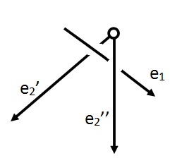
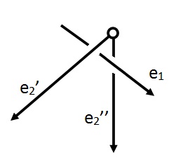
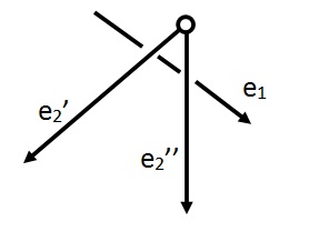
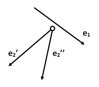
(a)	(b)	(c)	(d)

Figure 1. Edge and elbow embedding

We can think of  $\{e_{1},\Lambda\}$   as forming a (disconnected) abstract linkage  ${\mathcal{T}}_{\Gamma}=(V,E)$,  so as in §3.1, for each embedding  $\mathbf{x}:V\to{\mathbb{R}}^{3}$   of  ${\mathcal{T}}_{\Gamma}$   in space we have two invariants  $\phi_{\xi^{\prime}}(\mathbf{x}),\phi_{\xi^{\prime\prime}}(\mathbf{x})\in{\mathbb{Z}}/3=\{-1,0,1\}$   –  namely, the linking numbers of  $\mathbf{x}(e_{1})$   with  $\mathbf{x}(e_{2}^{\prime})$   and of  $\mathbf{x}(e_{1})$   with  $\mathbf{x}(e_{2}^{\prime\prime})$,  respectively. Together they yield  $\vec{\phi}(\mathbf{x})\in({\mathbb{Z}}/3)^{{\mathcal{P}}}={\mathbb{Z}}/3\times{\mathbb{Z}}/3$.

For example, if in the embedding $\mathbf{x}$ shown in Figure 1(a) we have chosen the orientation for  ${\mathbb{R}}^{3}$   so as to have linking numbers  $\vec{\phi}(\mathbf{x})=(+1,-1)$,  say, then Figure 1(b) will have  $\vec{\phi}(\mathbf{x})=(-1,+1)$.

On the other hand, for the embedding of Figure 1(c) we have  $\vec{\phi}(\mathbf{x})=(-1,-1)$,  while for Figure 1(d) we have  $\vec{\phi}(\mathbf{x})=(0,0)$,  since the nearest points to  $\mathbf{x}(e_{1})$   on  $\mathbf{x}(e_{2}^{\prime})$   or  $\mathbf{x}(e_{2}^{\prime\prime})$   are not interior points of the latter.

Thus we see that the immersed configuration represented by Figure 2(a), in which  $\mathbf{x}(e_{1})$   passes through the vertex  $\mathbf{x}(v)$,  but is not coplanar with  $\mathbf{x}(e_{2}^{\prime})$   and  $\mathbf{x}(e_{2}^{\prime\prime})$,  has two preimages in the blowup  $\underline{\operatorname{Emb}}({\mathcal{T}}_{\Gamma})=\underline{{\mathcal{C}}}(\Gamma)$,  one of which corresponds to Figure 1(a) (with invariants  $(+1,+1)$),  while the other preimage corresponds to both Figures 1(c)-(d), under the equivalence relation of §3.2, since we can have Cauchy sequences of either type converging to 2(a).

On the other hand, the immersed configuration represented by Figure 2(b), in which  $\mathbf{x}(e_{1})$   passes through the vertex  $\mathbf{x}(v)$,  and all edges are coplanar, is represented by three distinct types of inequivalent Cauchy sequences in  ${\mathcal{C}}({\Gamma})$,  corresponding to Figure 1(a), Figure 1(b), and Figure 1(c)-(d), respectively. Thus it has three preimages in the blowup  $\underline{\operatorname{Emb}}({\mathcal{T}}_{\Gamma})=\underline{{\mathcal{C}}}(\Gamma)$.  This is the reason we used invariants in  ${\mathbb{Z}}/3$,  rather than  ${\mathbb{Z}}/2$.

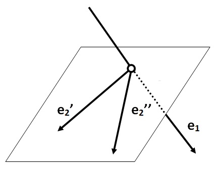
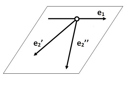
(a)	(b)

Figure 2. Virtual edge and elbow configuration

One further situation we must consider in analyzing the edge-elbow linkage is when two or more edges coincide:

1. When only  $\mathbf{x}(e_{2}^{\prime})$   and  $\mathbf{x}(e_{2}^{\prime\prime})$   coincide  –  that is, the elbow is closed  –  we still have the two cases described in Figure 2.

2. If  $\mathbf{x}(e_{1})$   coincides with  $\mathbf{x}(e_{2}^{\prime})$,  say, with  $\mathbf{x}(v)$   internal to  $\mathbf{x}(e_{1})$,  the pre-image in  $\underline{\operatorname{Emb}}({\mathcal{T}}_{\Gamma})$   is a single virtual configuration (since all cases are identified under $\sim$). This is true whether or not the elbow is closed.

4.3.

Two elbows. Next consider two elbows:  $\Lambda_{1}$,  consisting of two edges  $e_{1}^{\prime}$   and  $e_{1}^{\prime\prime}$   with a common vertex  $v_{1}$   and  $\Lambda_{2}$,  where two other edges  $e_{2}^{\prime}$   and  $e_{2}^{\prime\prime}$   are joined at the vertex  $v_{2}$,  as in Figure 3:

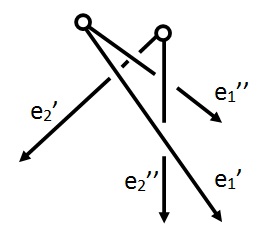
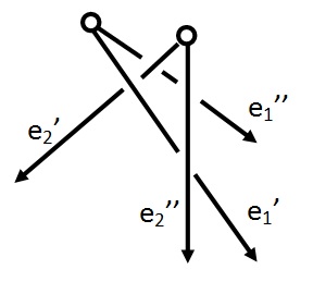
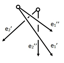
(a)	(b)	(c)

Figure 3. Double elbow configurations

Now we have four two-edge configurations, consisting of pairs of edges  $(e_{1}^{\prime},\,e_{2}^{\prime})$,   $(e_{1}^{\prime},\,e_{2}^{\prime\prime})$,   $(e_{1}^{\prime\prime},\,e_{2}^{\prime})$   and  $(e_{1}^{\prime\prime},\,e_{2}^{\prime\prime})$   respectively, so  $\vec{\phi}$   takes value in  $({\mathbb{Z}}/3)^{{\mathcal{P}}}=({\mathbb{Z}}/3)^{4}$.

For example, in the embedding of Figure 3(a) we have  $\vec{\phi}(\mathbf{x}):=(+1,+1,+1,-1)$,  in Figure 3(b) we then have  $\vec{\phi}(\mathbf{x}):=(+1,-1,-1,-1)$,  while in Figure 3(c) we have  $\vec{\phi}(\mathbf{x}):=(+1,+1,+1,+1)$.

The virtual configuration we need to consider is one in which the vertices of the two elbows coincide. As in Section 4.2, we must consider a number of mutual positions in space, as in Figure 4.

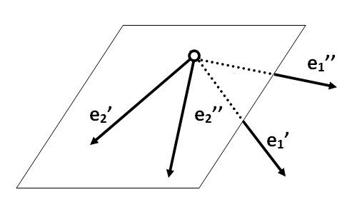
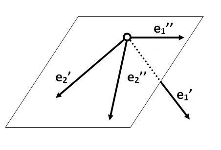
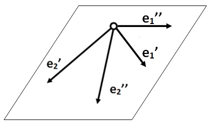
(a)	(b)	(c)

Figure 4. Virtual double elbow configuration

Assuming the edges  $\mathbf{x}(e_{2}^{\prime})$   and  $\mathbf{x}(e_{2}^{\prime\prime})$   do not coincide, they span a plane $E$. If at least one of the edges  $e_{1}^{\prime}$   and  $e_{1}^{\prime\prime}$   does not lie in $E$, as in Figure 4(a)-(b), we generally have three possibilities for the blow-up invariants: namely, the limits of the three cases shown in Figure 3, where case (c) (and a number of others) are identified with the case of the two elbows being disjoint. The same holds if all four edges lie in $E$, as in Figure 4(c).

On the other hand, if  $e_{1}^{\prime}$   and  $e_{1}^{\prime\prime}$   are on opposite sides of $E$, we cannot have the mutual positions described in Figure 3(b), so only two blow-up invariants can occur.

We do not consider here the more complicated cases when one or two of the elbows are closed, so that the edges  $e_{2}^{\prime}$   and  $e_{2}^{\prime\prime}$,  say, coincide (and thus we have no plane $E$)  –  even though similar considerations may be applied there.

5. Pairs of generalized intervals

Even for relatively simple linkage types  ${\mathcal{T}}_{\Gamma}$,  the global structure of the blow up  $\underline{\operatorname{Emb}}({\mathcal{T}}_{\Gamma})$   (or  $\underline{{\mathcal{C}}}(\Gamma)$)  can be quite complicated. However, the local structure is more accessible to analysis.

The simplest non-trivial case of a blow-up for a general linkage type  ${\mathcal{T}}_{\Gamma}$   occurs when two edges  $e^{\prime}$   and  $e^{\prime\prime}$   have a single intersection point $P$ interior to both  $\mathbf{x}(e^{\prime})$   and  $\mathbf{x}(e^{\prime\prime})$.  Such a configuration behaves locally like the completed configuration space of two (generalized) intervals in  ${\mathbb{R}}^{3}$,  which we analyze in this section.

5.A.    Two lines in ${\mathbb{R}}^{3}$

We begin with a linkage type  ${\mathcal{T}}_{\Gamma_{1}}$   of two lines  $\ell_{1}$   and  $\ell_{2}$.  In this case there is no length vector, so  $\Gamma_{1}={\mathcal{T}}_{\Gamma_{1}}$   and  ${\mathcal{C}}({\Gamma_{1}})=\operatorname{Emb}({\mathcal{T}}_{\Gamma_{1}})$.  Note that the convention of §1.3 implies that each line has a given orientation.

For simplicity, we first consider the case where the first line  $\ell_{1}$   is the (positively oriented) $x$-axis $\vec{\mathbf{x}}$, so we need to understand the choices of the second line  $\ell=\ell_{2}$   in  ${\mathbb{R}}^{3}$.

Inside the space ${\mathcal{L}}$ of oriented lines $\ell$ in  ${\mathbb{R}}^{3}$   (that is,  ${\mathcal{L}}={\mathcal{C}}({\Gamma_{0}})$,  where  $\Gamma_{0}$   consists of a single line) we have the subspace  ${\mathcal{L}}_{\vec{\mathbf{x}}}$   of lines intersecting the $x$-axis. We have  ${\mathcal{L}}_{\vec{\mathbf{x}}}=({\mathbb{R}}\times S^{2})/\sim$,  where  $(x,\vec{\mathbf{v}})\sim(x^{\prime},\vec{\mathbf{v}}^{\prime})$   for any  $x,x^{\prime}\in{\mathbb{R}}$   if and only if  $\vec{\mathbf{v}},\vec{\mathbf{v}}^{\prime}\in\{\pm\vec{\mathbf{e}}_{1}\}$,  with  $x\mapsto(x,0,0)$   sending ${\mathbb{R}}$ to  ${\mathbb{R}}^{3}$.  Moreover, we have a map  $\varphi:{\mathcal{C}}^{\operatorname{re}}({\Gamma_{1}})\to{\mathcal{L}}$   from the (unpointed) reduced configuration space  ${\mathcal{C}}^{\operatorname{re}}({\Gamma_{1}})=\operatorname{Emb}^{\operatorname{re}}({{\mathcal{T}}_{\Gamma_{1}}})$   for the original linkage, which is a homeomorphism onto  ${\mathcal{L}}\setminus{\mathcal{L}}_{\vec{\mathbf{x}}}$,  since any reduced embedding of  $\Gamma_{1}$   in  ${\mathbb{R}}^{3}$   is determined by a choice of an (oriented) line $\ell$ not intersecting the $x$-axis.

By taking an appropriate $\varepsilon$-tubular neighborhood of the two lines, we may assume that we have two $\varepsilon$-cylinders tangent to each other in  ${\mathbb{R}}^{3}$,  with one of them symmetric about the $x$-axis (see Figure 5). If we denote the space of such tangent cylinders by  $X_{\varepsilon}$,  we see that  $\operatorname{Emb}^{\operatorname{re}}({{\mathcal{T}}_{\Gamma_{1}}})$   is a disjoint union  $\bigsqcup_{\varepsilon>0}\,X_{\varepsilon}$.  Moreover, by re-scaling we see that all the spaces  $X_{\varepsilon}$   are homeomorphic, so in fact  $\operatorname{Emb}^{\operatorname{re}}({{\mathcal{T}}_{\Gamma_{1}}})\cong X_{1}\times(0,\infty)$,  say.

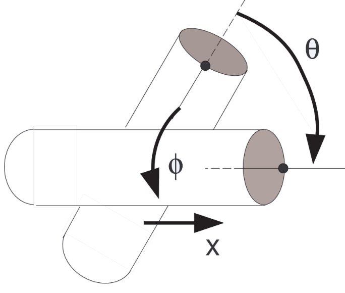
Figure 5. Tangent cylinders

Inside the space  $X_{1}$   we have a singular locus ${\mathcal{P}}$ of configurations where the two tangent cylinders are parallel. Thus  ${\mathcal{P}}\cong{\mathbf{S}}^{1}\times\{\pm 1\}$,  since such configurations are completely determined by the rotation $\phi$ of the cylinder  $T_{1}(\ell)$   around $\ell$ with respect to the cylinder  $T_{1}(\mathbf{x})$   around the $x$-axis, together with a choice of the orientation  $\pm 1$   of $\ell$ (relative to $\vec{\mathbf{x}}$).

The (open dense) complement  $X_{1}\setminus{\mathcal{P}}$   consists of configurations of a cylinder  $T_{1}(\ell)$   tangent at a single point $Q$ on the boundary of both cylinders. Such a configuration is determined by:

1. The projection  $x$   of the point $Q$ on $\vec{\mathbf{x}}$;

2. The angle $\theta$ between the (oriented) parallels to the respective axes $\vec{\mathbf{x}}$ and $\ell$ through $Q$; and

3. The rotation $\phi$ of $Q$ about $\vec{\mathbf{x}}$ (i.e., the rotation of the perpendicular  $\vec{xQ}$   to $\vec{\mathbf{x}}$ relative to $\vec{\mathbf{z}}$).

(see Figure 5).

Thus  $U:=X_{1}\setminus{\mathcal{P}}$   is diffeomorphic to the open manifold  ${\mathbb{R}}\times{\mathbf{S}}^{1}\times({\mathbf{S}}^{1}\setminus\{0,\pi\})$,  with global coordinates  $(x,\phi,\theta)$,  identifying $U$ with an open submanifold of the thickened torus  ${\mathbb{R}}^{1}\times{\mathbf{S}}^{1}\times{\mathbf{S}}^{1}$.  The boundary  ${\mathbb{R}}^{1}\times{\mathbf{S}}^{1}\times\{0,\pi\}$   of $U$ is identified in  $X_{1}$   with ${\mathcal{P}}$ by collapsing ${\mathbb{R}}^{1}$ to a point.

In summary,  $X_{1}$   is homeomorphic to the “tightened” torus  $({\mathbb{R}}^{1}\times{\mathbf{S}}^{1}\times{\mathbf{S}}^{1})/\sim$,  in which two opposite thickened circles (open annuli) are tightened to ordinary circles (see Figure 6). Thus  $X_{1}$   is homotopy equivalent to a torus  ${\mathbf{S}}^{1}\times{\mathbf{S}}^{1}$.

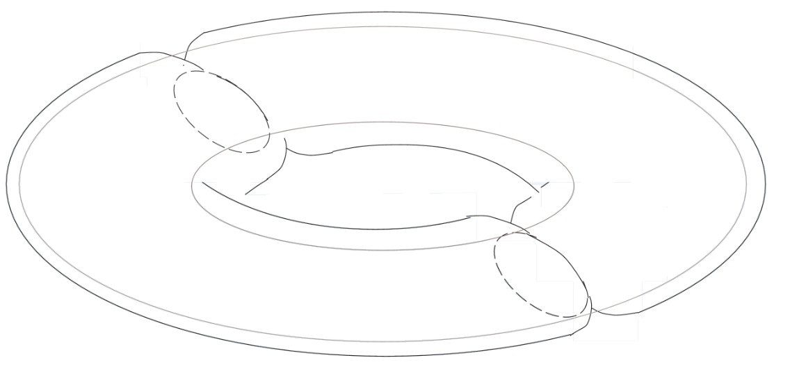
Figure 6. Tightened thickened torus

The full space of reduced embeddings  $\operatorname{Emb}^{\operatorname{re}}({{\mathcal{T}}_{\Gamma_{1}}})={\mathcal{C}}^{\operatorname{re}}({\Gamma_{1}})$   is still homotopy equivalent to  $X_{1}$,  and thus to  ${\mathbf{S}}^{1}\times{\mathbf{S}}^{1}$.  Its completion  $\widehat{\operatorname{Emb}}^{\operatorname{re}}({{\mathcal{T}}_{\Gamma_{1}}})$   allows configurations with  $\varepsilon=0$,  so it is a quotient of  $X_{1}\times[0,\infty)$.  When  $\theta\neq 0,\pi$,  we need no further identifications, since the new “virtual” configurations must still specify on which sides of each other the two lines touch. However, when $\ell$ is parallel to $\vec{\mathbf{x}}$, this has no meaning, so we find:

(5.1) $${}\widehat{\operatorname{Emb}}^{\operatorname{re}}({{\mathcal{T}}_{\Gamma_{1}}})~{}=~{}\widehat{{\mathcal{C}}}\,^{\operatorname{re}}(\Gamma_{1})~{}=~{}\left([0,\infty)\times{\mathbb{R}}^{1}\times{\mathbf{S}}^{1}\times{\mathbf{S}}^{1}\right)/\sim~{},$$

where  $(\varepsilon_{1},x_{1},\phi_{1},\theta_{1})\sim(\varepsilon_{2},x_{2},\phi_{2},\theta_{2})$:

1. for any  $x_{1},x_{2}\in{\mathbb{R}}^{1}$,  if  $\theta_{1}=\theta_{2}\in\{0,\pi\}$,   $\phi_{1}=\phi_{2}$,  and  $\varepsilon_{1}=\varepsilon_{2}>0$;

2. for any  $\phi_{1},\phi_{2}\in{\mathbf{S}}^{1}$   and  $x_{1},x_{2}\in{\mathbb{R}}^{1}$,  if  $\theta_{1}=\theta_{2}\in\{0,\pi\}$   and  $\varepsilon_{1}=\varepsilon_{2}=0$.

This is because  $(\varepsilon,\phi)$   serve as polar coordinates for the plane perpendicular to $\vec{\mathbf{x}}$ through the point of contact $Q$, and  $\varepsilon\cdot\phi$   is the length of the path rotating $\ell$ about $\vec{\mathbf{x}}$ when the two are parallel.

We still have a natural map  $\hat{\varphi}:\widehat{{\mathcal{C}}}\,^{\operatorname{re}}(\Gamma_{1})\to{\mathcal{L}}$   to the space of oriented lines in  ${\mathbb{R}}^{3}$,  taking a completed configuration to the location of  $\ell=\ell_{2}$, , but it is two-to-one on all points of  ${\mathcal{L}}_{\vec{\mathbf{x}}}$   (except $\vec{\mathbf{x}}$ itself), since a pair of intersecting lines corresponds to two different completed configurations. To distinguish between them, we need the following:

5.2 Definition.

As in §3.1, given two non-intersecting lines  $\ell_{1}$   and  $\ell_{2}$   in  ${\mathbb{R}}^{3}$,  their linking vector  $\vec{\mathbf{w}}=\vec{\mathbf{w}}_{(\ell_{1},\ell_{2})}$   is the shortest vector from a point on  $\ell_{1}$   to a point on  $\ell_{2}$,  perpendicular to their direction vectors  $\vec{\mathbf{u}}_{1}$   and  $\vec{\mathbf{u}}_{2}$.

When the lines are skew, $\vec{\mathbf{w}}$ is thus a multiple of  $\vec{\mathbf{u}}_{1}\times\vec{\mathbf{u}}_{2}$   by a scalar  $a\neq 0$,  and the linking number  $\operatorname{lk}_{(\ell_{1},\ell_{2})}$   of the two lines is  $\operatorname{sgn}(a)\in\{\pm 1\}$,  with  $\operatorname{lk}_{(\ell_{1},\ell_{2})}:=0$   when  $\ell_{1}\|\ell_{2}$   are parallel, as above.

By definition, points $\hat{\mathbf{x}}$ in the completed configuration space  $\widehat{{\mathcal{C}}}\,^{\operatorname{re}}(\Gamma_{1})$   correspond to (equivalence classes of) Cauchy sequences in the original space  ${\mathcal{C}}^{\operatorname{re}}({\Gamma_{1}})$,  and thus sequences of pairs of $\varepsilon$-cylinders tangent at a common point $Q$. Since we are not interested in configurations over the special point  $\vec{\mathbf{x}}\in{\mathcal{L}}$   (for which the two cylinders may be parallel), we may assume that the angle $\theta$ between the tangents  $t_{1}$   and  $t_{2}$   to the respective cylinders at $Q$ is not $0$ or $\pi$, so they determine a plane  $\operatorname{span}(t_{1},t_{2})$   with a specified normal direction $N$ (towards the second cylinder, having  $\ell_{2}$   as its axis, say). This is just the linking vector  $\vec{\mathbf{w}}_{(\ell_{1},\ell_{2})}$   defined above. The pair  $(t_{1},t_{2})$   converges along the Cauchy sequence to a pair of intersecting lines  $(\vec{\mathbf{x}},\ell)$,  and we define  $\hat{\varphi}(\hat{\mathbf{x}}):=\ell\in{\mathcal{L}}_{\vec{\mathbf{x}}}\subseteq{\mathcal{L}}$   extending the original homeomorphism  $\varphi:{\mathcal{C}}^{\operatorname{re}}({\Gamma_{1}})\to{\mathcal{L}}\setminus{\mathcal{L}}_{\vec{\mathbf{x}}}$.

Note that any  $\vec{\mathbf{x}}\neq\ell\in{\mathcal{L}}_{\vec{\mathbf{x}}}$   has two sources under $\hat{\varphi}$, corresponding to the two possible sides of the plane  $\operatorname{span}(\vec{\mathbf{x}},\ell)$   on which the cylinder around  $\ell_{2}$   could be.

In fact,  $\widehat{{\mathcal{C}}}\,^{\operatorname{re}}(\Gamma_{1})$   is homotopy equivalent to its “new part”  $C:=\widehat{{\mathcal{C}}}\,^{\operatorname{re}}(\Gamma_{1})\setminus{\mathcal{C}}^{\operatorname{re}}({\Gamma_{1}})$   under the map  $\psi:\widehat{{\mathcal{C}}}\,^{\operatorname{re}}(\Gamma_{1})\to C$   sending  $[(\varepsilon,x,\phi,\theta)]$   to  $[(0,x,\phi,\theta)]$.  Moreover, $C$ is homeomorphic to a twice-pinched torus, and so we have shown:

5.3 Proposition.

The reduced complete configuration space  $\widehat{{\mathcal{C}}}\,^{\operatorname{re}}(\Gamma_{1})$   of two lines in  ${\mathbb{R}}^{3}$   is homotopy equivalent to  ${\mathbf{S}}^{2}\vee{\mathbf{S}}^{2}\vee{\mathbf{S}}^{1}$.  Moreover, the map  $\hat{\varphi}:\widehat{{\mathcal{C}}}\,^{\operatorname{re}}(\Gamma_{1})\to{\mathcal{L}}$   is described up to homotopy by the map sending each of the two spheres to  ${\mathbf{S}}^{2}$,  with the pinch points (corresponding to the two oriented parallels to  $\ell_{1}$)  sent to the two poles.

For the general case of two oriented lines  $\ell_{1}$   and  $\ell_{2}$   in  ${\mathbb{R}}^{3}$,  assume first that in the linkage type  ${\mathcal{T}}_{\Gamma_{2}}$   the line  $\ell_{1}$   is framed  –  that is, equipped with a chosen normal direction $\vec{\mathbf{n}}$. The space of framed oriented lines in  ${\mathbb{R}}^{3}$   through the origin is  $\operatorname{SO}({3})$,  so the space  ${\mathcal{L}}^{\operatorname{fr}}$   of all framed oriented lines is given as for ${\mathcal{L}}$ by  $({\mathbb{R}}^{3}\times\operatorname{SO}({3}))/{\mathbb{R}}$,  and thus:

(5.4) $${}\widehat{{\mathcal{C}}}(\Gamma_{2})~{}=~{}{\mathbb{R}}^{3}\times\operatorname{SO}({3})\times{\mathbf{S}}^{1}\times\left([0,\infty)\times{\mathbb{R}}^{1}\times{\mathbf{S}}^{1}\times{\mathbf{S}}^{1}\right)/\sim~{},$$

where $\sim$ is generated by the equivalence relation of  ${\mathcal{C}}^{\operatorname{re}}({\Gamma_{1}})$   together with ${\mathbb{R}}$-translations along the first line  $\ell_{1}$.  To forget the orientations, we divide further by  ${\mathbf{S}}^{0}\times{\mathbf{S}}^{0}$,  and to forget the framing, we must further divide by the action of  ${\mathbf{S}}^{1}$   on $\vec{\mathbf{n}}$, so  $\widehat{{\mathcal{C}}}(\Gamma_{1})=\widehat{{\mathcal{C}}}(\Gamma_{2})/{\mathbf{S}}^{1}$.

5.5 Proposition.

When  $\Gamma_{1}$   consists as above of two (oriented) lines, the completion  $\widehat{{\mathcal{C}}}(\Gamma_{1})$   and the blow-up  $\underline{{\mathcal{C}}}(\Gamma_{1})$   of the configuration space are homeomorphic.

Proof.

The virtual configurations in  $\widehat{{\mathcal{C}}}(\Gamma_{1})$   are of two types, in which the two lines intersect or coincide. In the first case, the linking number of the two lines is the same constant in a tail of any two Cauchy sequences. In the second case, any Cauchy sequence is equivalent to one consisting only of parallel configurations, and therefore the linking numbers must be identified. ∎

5.B.    Other pairs of generalized intervals

In principle, all the other pairs of generalized intervals may be treated similarly. We shall merely point out the changes that need to be made in various special cases:

5.6.

Line and half-line. First, consider a linkage  $\Gamma_{3}={\mathcal{T}}_{\Gamma_{3}}$   consisting of an oriented line and a half-line  $\vec{\mathbf{p}}$.  For the pointed reduced embedding and configuration spaces, we may assume that  $\vec{\mathbf{p}}$   to be the positive direction of the $x$-axis, with endpoint  $\mathbf{0}\in{\mathbb{R}}^{3}$.

We see that  $\operatorname{Emb}^{\operatorname{re}}_{\ast}({{\mathcal{T}}_{\Gamma_{3}}})={\mathcal{C}}^{\operatorname{re}}_{\ast}({\Gamma_{3}})$   is the subspace of  $\operatorname{Imm}^{\operatorname{re}}({\mathcal{T}}_{\Gamma_{1}})$   consisting of oriented lines  $\ell=\ell_{2}$   in  ${\mathbb{R}}^{3}$   which do not intersect  $\vec{\mathbf{p}}$,  so in particular it is contained in  $W:=\operatorname{Imm}^{\operatorname{re}}({\mathcal{T}}_{\Gamma_{1}})\setminus\{\vec{\mathbf{x}}\}$.  Note that as in §5.A, the lines in $W$ can be globally parameterized by  $(\varepsilon,x,\phi,\theta)\in[0,\infty)\times{\mathbb{R}}^{1}\times{\mathbf{S}}^{1}\times{\mathbf{S}}^{1}$,  module the equivalence relation  $\theta\in\{0,\pi\}\Rightarrow{\mathbb{R}}^{1}\sim\ast$.  (The case  $\varepsilon=0$   allows the line to intersect $\vec{\mathbf{x}}$).

If we let

(5.7) $${}Z~{}:=~{}\{[(\varepsilon,x,\phi,\theta)]\in W\subseteq\left([0,\infty)\times{\mathbb{R}}^{1}\times{\mathbf{S}}^{1}\times{\mathbf{S}}^{1}\right)/\sim~{}:\ \varepsilon=0~{}\Rightarrow~{}x\leq 0\}$$

denote the subspace of  $W\subset\operatorname{Imm}^{\operatorname{re}}({\mathcal{T}}_{\Gamma_{1}})$   consisting of lines which do not intersect  $(0,\infty)\subseteq\vec{\mathbf{p}}$,  we see that the completed configuration space  $\widehat{\operatorname{Emb}}^{\operatorname{re}}_{\ast}({{\mathcal{T}}_{\Gamma_{3}}})=\widehat{{\mathcal{C}}}_{\ast}^{\operatorname{re}}(\Gamma_{3})$   is the pushout:

(5.8)

where $f$ is just the inclusion (using the same coordinates for source and target).

The quotient map  $q_{\Gamma_{3}}:\widehat{{\mathcal{C}}}_{\ast}^{\operatorname{re}}(\Gamma_{3})\to\operatorname{Imm}^{\operatorname{re}}({\mathcal{T}}_{\Gamma_{3}})=\operatorname{Imm}^{\operatorname{re}}({\mathcal{T}}_{\Gamma_{1}})$   of §2.7 is induced by the quotient map  $q_{\Gamma_{1}}:\widehat{{\mathcal{C}}}\,^{\operatorname{re}}(\Gamma_{1})\to\operatorname{Imm}^{\operatorname{re}}({\mathcal{T}}_{\Gamma_{1}})$   and the inclusion  $Z\hookrightarrow\operatorname{Imm}^{\operatorname{re}}({\mathcal{T}}_{\Gamma_{1}})$.

For the unreduced case, as above we first let  ${\mathcal{T}}_{\Gamma_{4}}$   consist of an oriented framed pair of line and half-line, so  $\widehat{{\mathcal{C}}}_{\ast}(\Gamma_{4})\cong\widehat{{\mathcal{C}}}_{\ast}^{\operatorname{re}}(\Gamma_{3})\times\operatorname{Spin}({3})\times{\mathbf{S}}^{1}$   (with the natural basepoint), and  $\widehat{{\mathcal{C}}}_{\ast}(\Gamma_{3})$   is obtained from  $\widehat{{\mathcal{C}}}_{\ast}(\Gamma_{4})$   by dividing out by a suitable action of  ${\mathbf{S}}^{1}\times{\mathbf{S}}^{1}$.

5.9 Remark.

The discussion above carries over essentially unchanged to a linkage  ${\mathcal{T}}_{\Gamma_{5}}$   consisting of an oriented line  $L_{1}$   and a finite segment $I$: in the reduced case, we assume  $I=[0,a]$   and then replace the conditions  $x\leq 0$   and  $0<x$   in  (5.7)   and  (5.8)   with  $x\not\in(0,a)$   and  $x\in(0,a)$,  respectively.

This is the first example where the moduli function  $\lambda_{{\mathcal{T}}_{\Gamma}}:\operatorname{Emb}({\mathcal{T}}_{\Gamma_{5}})\to{\mathbb{R}}^{1}$   is defined. However, all the embedding configuration spaces  ${\mathcal{C}}({\Gamma_{5}})$   are homoeomorphic to each other, and in fact  $\operatorname{Emb}({\mathcal{T}}_{\Gamma_{5}})\cong{\mathcal{C}}({\Gamma_{5}})\times(0,\infty)$.

5.10.

Two half-lines. Let  ${\mathcal{T}}_{\Gamma_{6}}$   be a linkage consisting of two oriented half-lines $\vec{\mathbf{p}}$ and $\vec{\mathbf{q}}$. For the reduced pointed space of embeddings  $\operatorname{Emb}^{\operatorname{re}}_{\ast}({{\mathcal{T}}_{\Gamma_{6}}})={\mathcal{C}}^{\operatorname{re}}_{\ast}({\Gamma_{6}})$,  we now assume as before that  $\vec{\mathbf{p}}$   is the positive half of the $x$-axis $X$, so each point  $\mathbf{x}\in\operatorname{Emb}^{\operatorname{re}}_{\ast}({{\mathcal{T}}_{\Gamma_{6}}})$   is determined by a choice of the vector $\vec{\mathbf{v}}$ from the end point of the $\vec{\mathbf{q}}$ to the origin (i.e., the end point of $\vec{\mathbf{p}}$), and the direction vector $\vec{\mathbf{w}}$ of the $\vec{\mathbf{q}}$. Thus  $\operatorname{Emb}^{\operatorname{re}}_{\ast}({{\mathcal{T}}_{\Gamma_{6}}})$   embeds as  $(\vec{\mathbf{v}},\vec{\mathbf{w}})$   in  ${\mathbb{R}}^{3}\times{\mathbf{S}}^{2}_{({2})}$.

The only virtual configurations we need to consider are when $\vec{\mathbf{p}}$ and $\vec{\mathbf{v}}$ are not collinear, and span a plane $E$ containing $\vec{\mathbf{p}}$ and $\vec{\mathbf{q}}$. In this case $\vec{\mathbf{w}}$ is determined by a single rotation parameter  $\theta=\theta_{\vec{\mathbf{v}}}$   (relative to $\vec{\mathbf{p}}$), and there are  $\theta_{0}<\theta_{1}$   such that $\vec{\mathbf{q}}$ intersects $\vec{\mathbf{p}}$ if and only if  $\theta_{0}<\theta\leq\theta_{1}$.  Thus we have an arc  $\gamma=\gamma_{\vec{\mathbf{v}}}$   in  ${\mathbf{S}}^{2}_{({2})}$   of values for $\vec{\mathbf{w}}$ for which we have two virtual configurations in  $\widehat{\operatorname{Emb}}({\mathcal{T}}_{\Gamma_{6}})$,  yielding an embedding of the compactification  $\overline{{\mathbf{S}}^{2}_{({2})}\setminus\gamma_{\vec{\mathbf{v}}}}$   of a sphere with a slit removed in  $\widehat{\operatorname{Emb}}({\mathcal{T}}_{\Gamma_{6}})$.  Since all such compactifications are homeomorphic to  $\overline{{\mathbf{S}}^{2}_{({2})}\setminus\gamma}$,  say, we see that

$$\widehat{\operatorname{Emb}}({\mathcal{T}}_{\Gamma_{6}})~{}\cong~{}X\times{\mathbf{S}}^{2}_{({2})}~{}\cup({\mathbb{R}}^{3}\setminus X)\times\overline{{\mathbf{S}}^{2}_{({2})}\setminus\gamma}~{}.$$

Since  $\overline{{\mathbf{S}}^{2}_{({2})}\setminus\gamma}$   is contractible, by collapsing the $x$ axis $X$ to the origin we see that  $\widehat{\operatorname{Emb}}({\mathcal{T}}_{\Gamma_{6}})\simeq{\mathbf{S}}^{2}$.

5.11 Remark.

Along the way our analysis showed that for all types of pairs of generalized intervals the maps  $\widetilde{\Phi}:\widehat{\operatorname{Emb}}({\mathcal{T}}_{\Gamma})\to\underline{\operatorname{Emb}}({\mathcal{T}}_{\Gamma})$   and  $\widetilde{\Phi}:\widehat{{\mathcal{C}}}(\Gamma)\to\underline{{\mathcal{C}}}(\Gamma)$   of  (3.7)  - (3.8)   are homeomorphisms  –  that is, the completed configuration space is identical with the blow-up. This does not hold for more general linkage types  –  see §9.4 below.

6. Lines in ${\mathbb{R}}^{3}$

In order to deal with more complex virtual configurations, we need to understand the completed configuration spaces of $n$ lines in  ${\mathbb{R}}^{3}$.

The configuration space of (non-intersecting) skew lines in  ${\mathbb{R}}^{3}$   have been studied from several points of view (see [CP, P] and the surveys in [DV, Vi]). However, here we are mainly interested in the completion of this space, and in particular in the virtual configurations where the lines “intersect” (but still retain the information on their mutual position, as before).

6.1 Definition.

As above, let  ${\mathcal{L}}={\mathcal{C}}({\Gamma_{0}})$   denote the space of oriented lines in  ${\mathbb{R}}^{3}$,  and ${\mathcal{N}}$ the space of all lines in  ${\mathbb{R}}^{3}$   (so we have a double cover  ${\mathcal{L}}\to\to{\mathcal{N}}$).

An oriented line is determined by a choice of a basepoint in  ${\mathbb{R}}^{3}$   and a vector in  $S^{2}$,  and since the basepoint is immaterial, the space ${\mathcal{L}}$ of all oriented lines in  ${\mathbb{R}}^{3}$   is  $({\mathbb{R}}^{3}\times S^{2})/{\mathbb{R}}$,  where ${\mathbb{R}}$ acts by translation of the basepoint along $\ell$. Alternatively, we can associate to each oriented line $\ell$ the pair  $(\vec{\mathbf{v}},\mathbf{x})$,  where  $\vec{\mathbf{v}}\in S^{2}$   is the unit direction vector of $\ell$, and $\mathbf{x}\in{\mathbb{R}}^{3}$ is the nearest point to the origin on $\ell$, allowing us to identify:

(6.2) $${}{\mathcal{L}}~{}\cong~{}\{(\vec{\mathbf{v}},\mathbf{x})\in S^{2}\times{\mathbb{R}}^{3}~{}:\ \mathbf{x}\cdot\vec{\mathbf{v}}=0\}~{}.$$

If  $\Gamma_{n}={\mathcal{T}}_{\Gamma_{n}}$   is the linkage consisting of $n$ oriented lines, we thus have an isometric embedding $\pi$ of  ${\mathcal{C}}({\Gamma_{n}})=\operatorname{Emb}({\mathcal{T}}_{\Gamma_{n}})$   in the product  ${\mathcal{L}}^{\times{n}}$,  which extends to a surjection  $\hat{\pi}:\widehat{\operatorname{Emb}}({\mathcal{T}}_{\Gamma_{n}})\to{\mathcal{L}}^{\times{n}}$   (no longer one-to-one).

Denote by  ${\mathcal{L}}^{\times{n}}_{\mathbf{0}}$   the subspace of  ${\mathcal{L}}^{\times{n}}$   consisting of all those lines passing through the origin (that is, with  $\mathbf{x}=\vec{\mathbf{0}}$),  so  ${\mathcal{L}}^{\times{n}}_{\mathbf{0}}\cong(S^{2})^{n}$,  and let  $\widehat{{\mathcal{E}}}_{n}:=\hat{\pi}^{-1}({\mathcal{L}}^{\times{n}}_{\mathbf{0}})$.  Thus  $\widehat{{\mathcal{E}}}_{n}$   consists of all (necessarily virtual) configurations of $n$ lines passing through the origin.

We denote by $\Sigma$ the subspace of  ${\mathcal{L}}^{\times{n}}\subseteq(S^{2}\times{\mathbb{R}}^{3})^{n}$   for which at least two of the $n$ unit vectors in  $S^{2}$   are parallel:

$$\Sigma~{}:=~{}\{(\vec{\mathbf{v}}_{1},\mathbf{x}_{1}\dotsc,\vec{\mathbf{v}}_{n},\mathbf{x}_{n})\in S^{2})^{n}~{}:\ \exists 1\leq i<j\leq n\ \exists 0\neq\lambda\in{\mathbb{R}},\ \vec{\mathbf{v}}_{i}=\lambda\vec{\mathbf{v}}_{j}\}~{}.$$

Finally, let  $\hat{\Sigma}:=\hat{\pi}^{-1}(\Sigma)$   denote the corresponding singular subspace of  $\widehat{\operatorname{Emb}}({\mathcal{T}}_{\Gamma_{n}})$.

6.3 Proposition.

There is a deformation retract  $\rho:\widehat{\operatorname{Emb}}({\mathcal{T}}_{\Gamma_{n}})\to\widehat{{\mathcal{E}}}_{n}$.

Proof.

For each  $t\in[0,1]$   we may use  (6.2)   to define a map  $h_{t}:{\mathcal{L}}^{\times{n}}\to{\mathcal{L}}^{\times{n}}$   by setting

$$h_{t}((\vec{\mathbf{v}}_{1},\mathbf{x}_{1}),\dotsc,(\vec{\mathbf{v}}_{n},\mathbf{x}_{n}))~{}:=~{}((\vec{\mathbf{v}}_{1},t\mathbf{x}_{1}),\dotsc,(\vec{\mathbf{v}}_{n},t\mathbf{x}_{n}))~{}.$$

For  $t>0$,   $h_{t}$   is equivalent to applying the $t$-dilitation about the origin in  ${\mathbb{R}}^{3}$   to each line in  ${\mathcal{T}}_{\Gamma_{n}}$.  Thus it takes the subspace  $\operatorname{Emb}({\mathcal{T}}_{\Gamma_{n}})$   of  ${\mathcal{L}}^{\times{n}}$   to itself, and therefore extends to a map  $\widehat{h}_{t}:\widehat{\operatorname{Emb}}({\mathcal{T}}_{\Gamma_{n}})\to\widehat{\operatorname{Emb}}({\mathcal{T}}_{\Gamma_{n}})$.

Now consider a Cauchy sequence  $\{P^{({i})}\}_{i=0}^{\infty}$   in  $\operatorname{Emb}({\mathcal{T}}_{\Gamma_{n}})$,  of the form

(6.4) $${}P^{({i})}~{}=~{}((\vec{\mathbf{v}}_{1}^{({i})},\mathbf{x}_{1}^{({i})}),\dotsc,(\vec{\mathbf{v}}_{n}^{({i})},\mathbf{x}_{n}^{({i})}))~{},$$

converging to a virtual configuration  $P\in\widehat{\operatorname{Emb}}({\mathcal{T}}_{\Gamma_{n}})$.  Choosing any sequence  $(t_{i})_{i=0}^{\infty}$   in  $(0,1]$   converging to $0$, we obtain a new Cauchy sequence  $\{h_{t_{i}}(P^{i})\}_{i=0}^{\infty}$   with

$$h_{t_{i}}(P^{({i})})~{}=~{}((\vec{\mathbf{v}}_{1}^{({i})},t_{i}\mathbf{x}_{1}^{({i})}),\dotsc,(\vec{\mathbf{v}}_{n}^{({i})},t_{i}\mathbf{x}_{n}^{({i})}))~{},$$

which is still a Cauchy sequence in  $\operatorname{Emb}({\mathcal{T}}_{\Gamma_{n}})$,  and furthermore  $\lim_{i\to\infty}~{}t_{i}\mathbf{x}_{j}^{({i})}=\mathbf{0}$   for all  $1\leq j\leq n$   since the vectors  $(\mathbf{x}_{1}^{({i})},\dotsc,\mathbf{x}_{n}^{({i})})$   have a common bound $K$ for all  $i\in{\mathbb{N}}$.  Thus  $\{h_{t_{i}}(P^{i})\}_{i=0}^{\infty}$   represents a virtual configuration  $P^{\prime}$   in  $\widehat{\operatorname{Emb}}({\mathcal{T}}_{\Gamma_{n}})$   with  $\pi(P^{\prime})\in{\mathcal{L}}^{\times{n}}_{\mathbf{0}}$,  and thus  $P^{\prime}\in\widehat{{\mathcal{E}}}_{n}$.  Moreover, choosing a different sequence  $(t_{i})_{i=0}^{\infty}$   yields the same  $P^{\prime}$.  Thus if we set  $\widehat{h}_{0}(P):=P^{\prime}$,  we obtain the required map  $\rho:=\widehat{h}_{0}:\widehat{\operatorname{Emb}}({\mathcal{T}}_{\Gamma_{n}})\to\widehat{{\mathcal{E}}}_{n}$,  as well as a homotopy  $H:\widehat{\operatorname{Emb}}({\mathcal{T}}_{\Gamma_{n}})\times[0,1]\to\widehat{\operatorname{Emb}}({\mathcal{T}}_{\Gamma_{n}})$   with  $H(P,t)=\widehat{h}_{t}(P)$   for  $t>0$   –  and thus  $H(-,1)=\operatorname{Id}$   –  and  $H(-,0)=\rho$.  ∎

6.5 Corollary.

The completed configuration space  $\widehat{\operatorname{Emb}}({\mathcal{T}}_{\Gamma_{n}})$   of $n$ oriented lines in  ${\mathbb{R}}^{3}$   is homotopy equivalent to the completed space  $\widehat{{\mathcal{E}}}_{n}$   of $n$ oriented lines through the origin.

7. Three lines in ${\mathbb{R}}^{3}$

Corollary 6.5 allows us to reduce the study of the homotopy type of the completed configuration space of $n$ (oriented) lines in  ${\mathbb{R}}^{3}$   to the that of the simpler subspace of $n$ lines through the origin (where we may fix  $\ell_{1}$   to be the $x$-axis).

7.1.

The case of two lines again. For  $n=2$,  the remaining (oriented) line  $\ell_{2}$   is determined by its direction vector  $\vec{\mathbf{v}}\in{\mathbf{S}}^{2}$,  which is aligned with  $\ell_{1}$   at the north pole, say, and reverse-aligned at the south pole. Since we need to take into account the linking number  $\pm 1\in{\mathbb{Z}}/2$  of  $\ell_{1}$   and  $\ell_{2}$,  we actually have two copies of  ${\mathbf{S}}^{2}$.  However, the north and south poles of these spheres, corresponding to the cases when  $\ell_{2}$   is aligned or reverse-aligned with  $\ell_{1}$,  must be identified as in Figure 7, so we see that  $\widehat{{\mathcal{E}}}_{2}\simeq{\mathbf{S}}^{2}\vee{\mathbf{S}}^{2}\vee{\mathbf{S}}^{1}$,  as in Proposition 5.3.

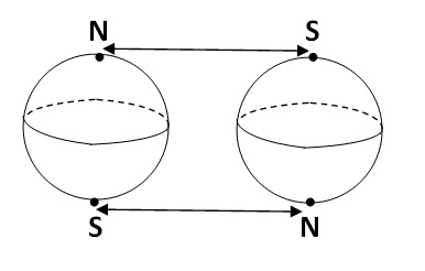
Figure 7. The completed configuration space  $\widehat{{\mathcal{E}}}_{2}$

7.2.

The cell structure for three lines.

For  $n=3$,  we again fix  $\ell_{1}$   to be the positively oriented $x$-axis. The remaining two lines  $\ell_{2}$   and  $\ell_{3}$   are determined by their two direction vectors  $(\vec{\mathbf{v}}_{2},\vec{\mathbf{v}}_{3})\in{\mathbf{S}}^{2}_{(1)}\times{\mathbf{S}}^{2}_{(2)}$.  Again all in all there are eight copies of  ${\mathbf{S}}^{2}\times{\mathbf{S}}^{2}$,  indexed by the triples of completed linking numbers  $\delta_{i,j}:=\phi_{(\ell_{i},\ell_{j})}=\pm 1$   for  $1\leq i<j\leq 3$   (see §3.2).

As in §7.1, there are identifications among these products of two spheres, which occur when at least one pair of lines is aligned or reverse-aligned: this takes place either in the diagonal  $\operatorname{diag}({\mathbf{S}}^{2}_{(1)}\times{\mathbf{S}}^{2}_{(2)})$   (when  $\ell_{2}$   and  $\ell_{3}$   are aligned), in the anti-diagonal  $-\operatorname{diag}({\mathbf{S}}^{2}_{(1)}\times{\mathbf{S}}^{2}_{(2)})$   (when  $\ell_{2}$   and  $\ell_{3}$   are reverse-aligned), or in one of the four subspaces of the form  ${\mathbf{S}}^{2}_{(1)}\times\{N\}$   (when  $\ell_{1}$   and  $\ell_{2}$   are aligned), and so on. Thus we have:

$$\widehat{{\mathcal{E}}}_{3}~{}=~{}\left(\coprod_{1\leq i<j\leq 3}\ [{\mathbf{S}}^{2}_{(1)}\times{\mathbf{S}}^{2}_{(2)}]_{\delta_{i,j}}\right)/\sim~{}.$$

The four special points  $(N,N),\,(N,S),\,(S,N),\,(S,S)$,  each appearing in three of the identification spheres for each of the eight indices  $\delta_{i,j}$,  must also be identified, as indicated by the arrows in Figure 8.

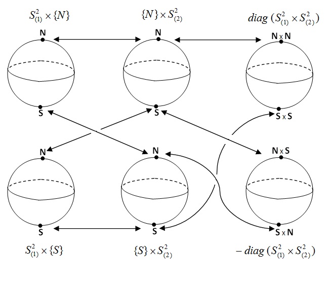
Figure 8. Subspaces of  $[{\mathbf{S}}^{2}_{(1)}\times{\mathbf{S}}^{2}_{(2)}]_{\delta_{i,j}}$   where identifications occur

This suggests the following cell structure for  $\widehat{{\mathcal{E}}}_{3}$,  in which we decompose each of the eight copies of  ${\mathbf{S}}^{2}\times{\mathbf{S}}^{2}$   into $8$ four-dimensional cells, as follows:

Using cylindrical coordinates  $(\theta,t)$,  we think of  ${\mathbf{S}}^{2}$   as a cylinder with the top and bottom identified to a point, (i.e., a square with top and bottom collapsed and vertical sides identified levelwise). As a result,  ${\mathbf{S}}^{2}\times{\mathbf{S}}^{2}$   may be viewed as a product of the  $(t_{1},t_{2})$ -square with the  $(\theta_{1},\theta_{2})$ -square (with suitable identifications), and its eight cells are obtained by as products of their respective subdivisions, indicated in Figure 9. Note that it is convenient to replace the  $(\theta_{1},\theta_{2})$ -square by a parallelogram, so the opposite diagonal edges correspond to  $\theta_{1}=\theta_{2}$   (identified with each other). The horizontal edges are also identified pointwise.

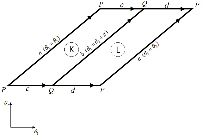
	$\times$
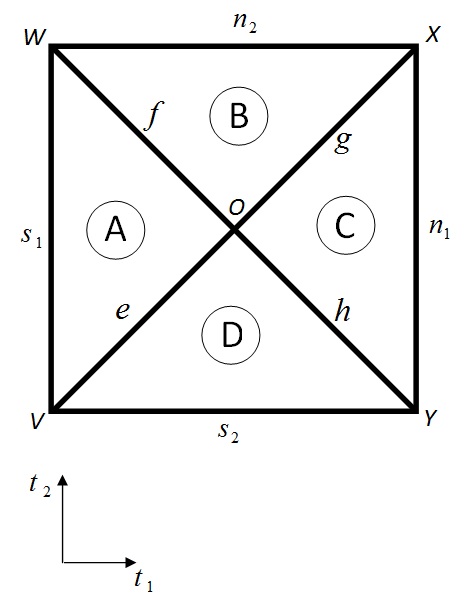
(a)  $(\theta_{1},\theta_{2})\in{\mathbf{S}}^{1}\times{\mathbf{S}}^{1}$		(b)   $(t_{1},t_{2})\in[-1,1]\times[-1,1]$

Figure 9. ${\mathbf{S}}^{2}_{(1)}\times{\mathbf{S}}^{2}_{(2)}$  in double cylindrical coordinates

Thus each of the eight copies of  ${\mathbf{S}}^{2}\times{\mathbf{S}}^{2}$   decomposes into $8$ $4$-dimensional cells:  $A\times K,B\times K,C\times K,D\times K,A\times L,B\times L,C\times L,D\times L$.

However, there are certain collapses in the lower-dimensional products, all deriving from the fact that when  $t_{i}=\pm 1$   (at either end of the cylinder), the variable  $\theta_{i}$   has no meaning, so under the quotient map

$$q~{}=~{}q_{(1)}\times q_{(2)}~{}:~{}\left({\mathbf{S}}^{1}_{(1)}\times{\mathbf{S}}^{1}_{(2)}\right)\times\left([-1,1]_{(1)}\times[-1,1]_{(2)}\right)~{}\to\to~{}{\mathbf{S}}^{2}_{(1)}\times{\mathbf{S}}^{2}_{(2)}$$

any point  $(\theta_{1},\theta_{2},-1,t_{2})$   is sent to  $(S_{(1)},q_{(2)}(\theta_{2},t_{2}))$,  where  $S_{(1)}$   is the south pole in the first sphere  ${\mathbf{S}}^{2}_{(1)}$,  and so on. Thus:

1. The ostensibly $3$-dimensional cell  $K\times s_{1}$   is collapsed horizontally under $q$ to the $2$-cell  $S_{(1)}\times{\mathbf{S}}^{2}_{(2)}$.  Note that the same $2$-cell is also represented by  $a\times s_{1}$   and  $b\times s_{1}$.

   Similarly  $q(L\times s_{1})=S_{(1)}\times{\mathbf{S}}^{2}_{(2)}$   and  $q(K\times n_{1})=q(L\times n_{1})=N_{(1)}\times{\mathbf{S}}^{2}_{(2)}$.

2. On the other hand,  $K\times s_{2}$   is collapsed horizontally to the $2$-cell  $c\times s_{2}$,  and similarly  $q(K\times n_{2})=q(c\times n_{2})$,   $q(L\times s_{2})=q(d\times s_{2})$,  and  $q(L\times n_{2})=q(d\times n_{2})$.

3. The sum  $(c\cup d)\times s_{2}$   is identified under $q$ with  ${\mathbf{S}}^{2}_{(1)}\times S_{(2)}$,  which is also represented by  $a\times s_{2}$   or  $b\times s_{2}$.

   Similarly,  $q(c\cup d)\times n_{2})=q(a\times s_{2})=q(b\times s_{2})={\mathbf{S}}^{2}_{(1)}\times N_{(2)}$.

4. The two $2$-cells  $c\times s_{1}$   and  $d\times s_{1}$   are both collapsed under $q$ to the $1$-cell  $S_{(1)}\times H$,  where $H$ is the longitude  $\theta_{2}=0$   in  ${\mathbf{S}}^{2}_{(2)}$.  Similarly,  $q(c\times n_{1})=q(d\times n_{1})=N_{(1)}\times H$.   $c\times n_{1}$,  and  $d\times n_{1}$

5. Since $V$ corresponds to the pair of south poles  $(S_{(1)},S_{(2)})$   in  ${\mathbf{S}}^{2}_{(1)}\times{\mathbf{S}}^{2}_{(2)}$,   $K\times V$   and  $L\times V$   are collapsed to a single point  $(S_{(1)},S_{(2)})$.

   Similarly,  $q(K\times W)=q(L\times W)=(S_{(1)},N_{(2)})$,   $q(K\times X)=q(L\times X)=(N_{(1)},N_{(2)})$,  and  $q(K\times Y)=q(L\times Y)=(N_{(1)},S_{(2)})$.

In addition, there are identifications among cells associated to the eight $2$-spheres indexed by  $(\delta_{1,2},\,\delta_{1,3},\,\delta_{2,3})\in({\mathbb{Z}}/3)^{3}$.  These occur only for the $0$-, $1$-, and $2$-cells, when at least two of  $\ell_{1}$,   $\ell_{2}$,  and  $\ell_{3}$   are aligned, so  $\delta_{i,j}=0$.  The resulting identifications are as follows:

1. The two $2$-cells  $a\times e$,  and  $a\times g$   consist of pairs of points  $(t_{i},\theta_{i})$    ($i=1,2$)   with  $t_{1}=t_{2}$   and  $\theta_{1}=\theta_{2}$,  so at all points in these cells  $\ell_{2}$   and  $\ell_{3}$   are aligned. Therefore,  $\delta_{2,3}=0$,  or equivalently, the corresponding cells in the two products  ${\mathbf{S}}^{2}\times{\mathbf{S}}^{2}$   indexed by the triples  $(\delta_{1,2},\delta_{1,3},+1)$   and  $(\delta_{1,2},\delta_{1,3},-1)$   are identified, for each of the four choices of  $(\delta_{1,2},\delta_{1,3})\in\{\pm 1\}^{2}$.

2. Similarly,  $b\times f$,  and  $b\times h$   consist of pairs of points  $(t_{i},\theta_{i})$    ($i=1,2$)   with  $t_{1}=-t_{2}$   and  $\theta_{1}=\theta_{2}$,  so  $\ell_{2}$   and  $\ell_{3}$   are reverse-aligned, and again the corresponding cells indexed by the triples  $(\delta_{1,2},\delta_{1,3},+1)$   and  $(\delta_{1,2},\delta_{1,3},-1)$   are identified.

3. The $2$-cell  $a\times n_{1}$   (identified with  $b\times n_{1}$   consist of pairs of points with  $t_{1}=+1$,  so  $\ell_{2}$   is aligned with  $\ell_{1}$   and the corresponding cells indexed by the triples  $(+1,\delta_{1,3},\delta_{2,3})$   and  $(-1,\delta_{1,3},\delta_{2,3})$   are identified.

4. The $2$-cell  $a\times s_{1}=b\times s_{1}$   consist of pairs of points with  $t_{1}=-1$,  so  $\ell_{2}$   is reverse-aligned with  $\ell_{1}$   and the corresponding cells indexed by the triples  $(+1,\delta_{1,3},\delta_{2,3})$   and  $(-1,\delta_{1,3},\delta_{2,3})$   are identified.

5. The two $2$-cells  $c\times n_{2}$,  and  $d\times n_{2}$   consist of pairs of points with  $t_{2}=+1$,  so  $\ell_{3}$   is aligned with  $\ell_{1}$   and the corresponding cells indexed by the triples  $(\delta_{1,2},+1,\delta_{2,3})$   and  $(\delta_{1,2},-1,\delta_{2,3})$   are identified.

6. The two $2$-cells  $c\times s_{2}$,  and  $d\times s_{2}$   consist of pairs of points with  $t_{2}=-1$,  so  $\ell_{3}$   is reverse-aligned with  $\ell_{1}$   and the corresponding cells indexed by the triples  $(\delta_{1,2},+1,\delta_{2,3})$   and  $(\delta_{1,3},-1,\delta_{2,3})$   are identified.

7. From (a) we see that the $1$-cell  $a\times O$   indexed by $(\delta_{1,2},\delta_{1,3},+1)$   and  $(\delta_{1,2},\delta_{1,3},-1)$   are identified, and similarly for  $P\times e$   and  $P\times g$.

8. From (b) we see likewise that the $1$-cells  $b\times O$,   $Q\times f$,  and  $Q\times h$   indexed by $(\delta_{1,2},\delta_{1,3},+1)$   and  $(\delta_{1,2},\delta_{1,3},-1)$   are also identified.

9. From (c) and (d) we see that the $1$-cells  $P\times s_{1}=Q\times s_{1}$,   $P\times n_{1}=Q\times n_{1}$,  indexed by  $(+1,\delta_{1,3},\delta_{2,3})$   and  $(-1,\delta_{1,3},\delta_{2,3})$   are identified.

10. From (e) and (f) we see that the $1$-cells  $P\times s_{2}$,   $Q\times s_{2}$,   $P\times n_{2}$,  and  $Q\times n_{2}$   indexed by  $(\delta_{1,2},+1,\delta_{2,3})$   and  $(\delta_{1,2},-1,\delta_{2,3})$   are identified.

11. Finally, all six $0$-cells  $P\times V=Q\times V$,   $P\times W=Q\times W$,   $P\times X=Q\times X$,   $P\times Y=Q\times Y$,   $P\times O$,  and  $Q\times O$   have all three lines  $\ell_{1}$,   $\ell_{2}$,  and  $\ell_{3}$   aligned or reverse-aligned, so  $\delta_{1,2}=\delta_{1,3}=\delta_{2,3}=0$   and all eight copies are identified.

Using this cell decomposition, we can easily verify that  $H_{4}\widehat{{\mathcal{E}}}_{3}~{}\cong~{}{\mathbb{Z}}^{8}$,  where for each of the eight products  ${\mathbf{S}}^{2}\times{\mathbf{S}}^{2}$   indexed by  $(\delta_{1,2},\delta_{1,3},\delta_{2,3})\in\{\pm 1\}^{3}$   we have a copy of ${\mathbb{Z}}$ generated by the fundamental $4$-cycle  $\gamma_{((\delta_{1,2},\delta_{1,3},\delta_{2,3})}:=(K+L)\times(A+B+C+D)$.  It is also clear that  $\widehat{{\mathcal{E}}}_{3}$   is connected, so  $H_{0}\widehat{{\mathcal{E}}}_{3}~{}\cong~{}{\mathbb{Z}}$.

We leave to the reader to verify that  $H_{3}(\widehat{{\mathcal{E}}}_{3};{\mathbb{Q}})~{}\cong~{}{\mathbb{Q}}^{6}$,   $H_{2}(\widehat{{\mathcal{E}}}_{3};{\mathbb{Q}})~{}\cong~{}{\mathbb{Q}}^{12}$.  and  $H_{1}(\widehat{{\mathcal{E}}}_{3};{\mathbb{Q}})~{}\cong~{}{\mathbb{Q}}^{9}$.

8. Chains in space

We can use the basic building blocks of Sections 6-7 to study some actual simple linkages, namely, those with a all vertices of valence $\leq 2$,  called chains. We begin with the simplest non-trivial example:

8.A.    Closed quadrilateral chains

Let $\Gamma$ be a closed quadrilateral chain with vertices $a$, $b$, $c$, and $d$, and length vector  $\vec{\ell}:=(\ell_{1},\ell_{2},\ell_{3},\ell_{4})=(|ab|,\,|bc|,\,|cd|,\,|ad|)$.  See Figure 10(b) We naturally assume the feasibility inequalities on $\vec{\ell}$ (generalized triangle inequalities), which guarantee that  $\widehat{{\mathcal{C}}}(\Gamma)$   is non-empty. In the generic case we have no equations of the form  $\ell_{1}=\pm\ell_{2}\pm\ell_{3}\pm\ell_{1}$   (which would allow the quadrilateral to be fully aligned).

In the reduced configuration space  ${\mathcal{C}}^{\operatorname{re}}_{\ast}({\Gamma})$   (cf. §1.5) we assume that $a$ is fixed at the origin $\vec{\mathbf{0}}$, the link  $ab$   is in the positive direction of the $x$-axis, so $b$ is fixed at the point  $\vec{{\mathbf{b}}}:=(\ell_{2},0)$.  If we mod out by the  ${\mathbf{S}}^{1}$ -action rotating the link  $ad$   in space about the $x$-axis, we obtain the space  $\overline{{\mathcal{C}}}^{\operatorname{re}}_{\ast}({\Gamma})$,  whose points are represented by embeddings of $\Gamma$ for which the link  $ad$   lies in the closed upper half plane ${\mathcal{H}}$ in the  ($x,y$)-plane.

8.1.

Local description of the singularities in $\widehat{{\mathcal{C}}}_{\ast}^{\operatorname{re}}(\Gamma)$.

Consider the simpler linkage $\Delta$ consisting of the two links  $ab$   and  $ad$   of lengths  $\ell_{1}$   and  $\ell_{4}$,  respectively, and with the distance  $bd$   contained in the closed interval  $I=[r,R]$   for  $r:=|\ell_{2}-\ell_{3}|$   and  $R=\ell_{2}+\ell_{3}$.  See Figure 10(a). The corresponding reduced planar configuration space, in which we require  $ab$   to lie on the $x$-axis and  $ad$   to lie in ${\mathcal{H}}$, is denoted by  $\widehat{{\mathcal{C}}}_{\ast}^{\operatorname{re}}(\Delta)$,  and there is a “forgetful map”  $\rho:\overline{{\mathcal{C}}}^{\operatorname{re}}_{\ast}({\Gamma})\to\widehat{{\mathcal{C}}}_{\ast}^{\operatorname{re}}(\Delta)$.

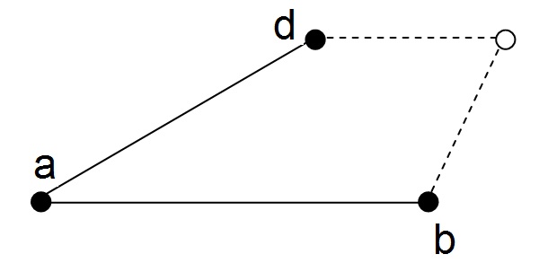
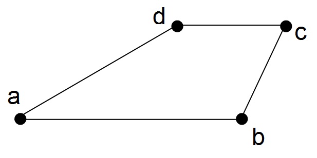
(a)  The submechanism $\Delta$	(b)  The $4$-chain $\Gamma$

Figure 10. The mechanisms $\Delta$ and $\Gamma$

For a configuration $\mathbf{x}$ in  $\overline{{\mathcal{C}}}^{\operatorname{re}}_{\ast}({\Gamma})$   the angle  $\angle bcd$   is determined by the locations of $b$ and $d$, and thus by the corresponding configuration  $\mathbf{y}=\rho(\mathbf{x})$,  and given any  $\mathbf{y}\in\widehat{{\mathcal{C}}}_{\ast}^{\operatorname{re}}(\Delta)$,  there is a unique  $\bar{\mathbf{x}}\in\rho^{-1}(\mathbf{y})$   in which $a$ and $c$ do not lie on the same side of the line through  $bd$   (unless $a$, $b$, and $d$ are aligned).

Given this $\bar{\mathbf{x}}$, in  ${\mathcal{C}}^{\operatorname{re}}_{\ast}({\Gamma})$   the elbow $\Lambda$ formed by $b$, $c$ and $d$ can rotate freely about  $bd$   (unless it is aligned). However, when we rotate $\Lambda$ from $\bar{\mathbf{x}}$ by  $180^{o}$   back into the  ($x,y$)-plane, the resulting (non-convex) configuration  $\bar{\mathbf{x}}^{\prime}$   may be self-intersecting, if the two opposite sides  $ab$   and  $cd$,  or else  $ad$   and  $bc$,  intersect in a point interior to one or the other.

By the analysis of planar quadrilateral configurations in [Fa, §1.3], we see that given such a self-intersecting planar configuration  $\bar{\mathbf{x}}^{\prime}$   of $\Gamma$, one may decrease one angle between adjacent links to obtain  $\mathbf{x}^{\prime\prime}\in{\mathcal{C}}^{\operatorname{re}}_{\ast}({\Gamma})$   (with angle  $0^{o}$,  with the two links aligned), after which the self-intersection disappears. Therefore, to study the cases in which $\Lambda$ cannot be fully rotated in  ${\mathbb{R}}^{3}$,  it suffices to consider the configurations  $\mathbf{x}^{\prime\prime}$   where one link is folded onto an adjacent link. We call a case where  $bc$   is folded back on  $ab$   a collineation  $(acb)$.  See Figure 11.

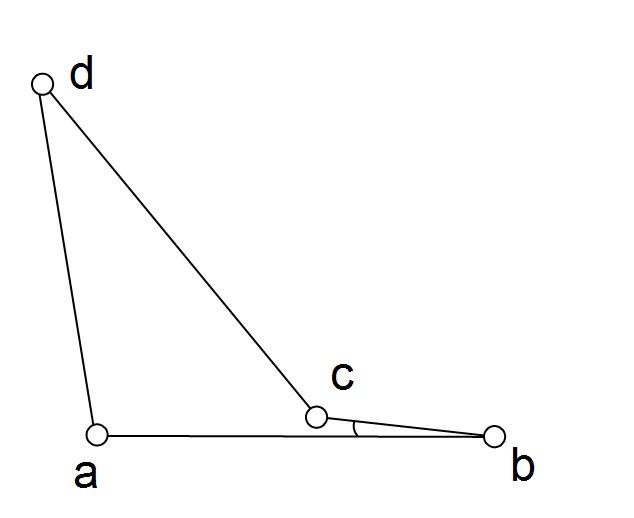
Figure 11. The collineation  $(acb)$

In the full reduced configuration space  ${\mathcal{C}}^{\operatorname{re}}_{\ast}({\Gamma})$   we have two angles associated to each configuration  $\bar{\mathbf{x}}\in\rho^{-1}(\mathbf{y})$   as above: $\theta$ determined by rotating $\Lambda$ about  $bd$,  and $\phi$ by rotating the resulting rigid spatial quadrilateral (of  $\overline{{\mathcal{C}}}^{\operatorname{re}}_{\ast}({\Gamma})$)  about the $x$-axis (assuming that $a$, $b$ and $d$ are not collinear).

Note that for all spatial quadrilaterals in  $\overline{{\mathcal{C}}}^{\operatorname{re}}_{\ast}({\Gamma})$   the rotation by $\phi$ is possible, and yields different spatial configurations of $\Gamma$ (since we are assuming $\Gamma$ cannot be fully aligned, because $\vec{\ell}$ is generic). Moreover, at a collineation  $\mathbf{x}^{\prime\prime}$   the full rotation by $\theta$ about  $bd$   is still allowed.

Any configuration  $\mathbf{x}^{\prime\prime}$   representing a collineation  $(acb)$,  say, has a neighborhood in the planar reduced configuration space  $\overline{{\mathcal{C}}}^{\operatorname{re}}_{\ast}({\Gamma})$   homeomorphic to an open interval  $(\varepsilon,\varepsilon)$   (with  $\mathbf{x}^{\prime\prime}$   itself identified with the midpoint $0$) such that in one half  $[0,\varepsilon)$   the full rotation by $\phi$ is allowed, while in the other half  $(-\varepsilon,0)$   the rotation by  $\phi=0^{o}$   is distinct in the completion (or blowup)  $\widehat{{\mathcal{C}}}_{\ast}^{\operatorname{re}}(\Gamma)$   from the rotation by  $\phi=360^{o}$,  in which the link  $cd$   touches  $ab$   on opposite sides. Similarly for  $(acd)$,   $(cab)$,  and  $(cad)$.

However, when  $\mathbf{x}^{\prime\prime}$   represents the collineation  $(abd)$   or  $(adb)$,  the rotation by $\phi$ about the $x$-axis is the same as the rotation by $\theta$ about  $bd$.  In this case we simply exchange the roles of  $bd$   and  $ac$   in defining  $\overline{{\mathcal{C}}}^{\operatorname{re}}_{\ast}({\Gamma})$,  and then the same analysis holds. Similarly for  $(bdc)$   and  $(dbc)$.

Therefore, in the reduced completed spatial configuration space  $\widehat{{\mathcal{C}}}_{\ast}^{\operatorname{re}}(\Gamma)$   (in which the only restriction is that side  $ab$   lies on the $x$ axis, with $a$ at the origin) a collineation configuration  $\mathbf{x}^{\prime\prime}$   has a neighborhood $U$ diffeomorphic (as a manifold with corners) to the union of the thickened torus  $U_{1}:=[0,\varepsilon)\times{\mathbf{S}}^{1}\times{\mathbf{S}}^{1}$   and split thickened torus  $U_{2}:=(-\varepsilon,0]\times[0^{o},360^{o}]\times{\mathbf{S}}^{1}$,  with  $(0,\theta,\phi)$   in  $U_{1}$   identified with  $(0,\theta,\phi)$   in  $U_{2}$   (and thus in particular  $(0,0^{o},\phi)$   and  $(0,360^{o},\phi)$   in  $U_{1}$   identified with  $(0,0^{o},\phi)=(0,360^{o},\phi)$   in  $U_{2}$).  The singular configuration  $\mathbf{x}^{\prime\prime}$   is parameterized by the point  $(0,0^{o},0^{o})$,  while the corresponding convex quadrilateral $\mathbf{x}$ is parameterized by  $(0,180^{o},0^{o})$.

8.2 Remark.

If one link is folded onto an adjacent link, we obtain a triangle with sides  $\ell_{i}$,   $\ell_{j}$,  and  $|\ell_{k}-\ell_{l}|$,  respectively (for  $\{i,j,k,l\}=\{1,2,3,4\}$).  For this to be possible, the three sides must satisfy the triangle inequalities. If we take into account the feasibility inequalities, these reduce to two cases:

(8.3) $${}\ell_{i}+\ell_{k}>\ell_{j}+\ell_{l}~{},\hskip 28.45274pt\ell_{j}+\ell_{k}>\ell_{i}+\ell_{l}~{},\hskip 28.45274pt\text{and}\hskip 5.69054pt\ell_{k}>\ell_{l}$$

or

(8.4) $${}\ell_{j}+\ell_{l}>\ell_{i}+\ell_{k}~{},\hskip 28.45274pt\ell_{i}+\ell_{l}>\ell_{j}+\ell_{k}~{},\hskip 28.45274pt\text{and}\hskip 5.69054pt\ell_{l}>\ell_{k}~{}.$$

8.5.

Global description of  ${\mathcal{C}}^{\operatorname{re}}_{\ast}({\Gamma})$.

As in the classical analysis of [MT],  $\widehat{{\mathcal{C}}}_{\ast}^{\operatorname{re}}(\Delta)$   may be identified with the intersection  $\widehat{\mathbf{e}\mathbf{h}}$   of the half-annulus  $A(d)$   in ${\mathcal{H}}$ about $\vec{{\mathbf{b}}}$ of radii  $r,R$   with the half circle  $B(d)$   of radius  $\ell_{4}$   about $\vec{\mathbf{0}}$ in the upper half-plane ${\mathcal{H}}$ (both describing possible locations for $d$). See Figure 12.

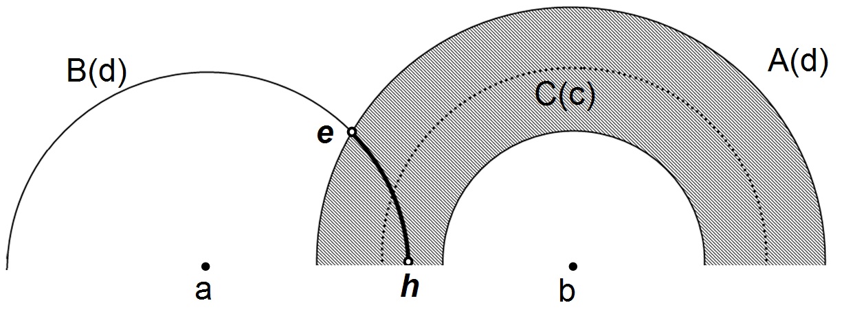
Figure 12. Reduced immersion space  $\widehat{{\mathcal{C}}}_{\ast}^{\operatorname{re}}(\Delta)$  

We may assume without loss of generality that

(8.6) $${}\ell_{4}<\ell_{1}>\ell_{2}>\ell_{3}~{},$$

so the collineations  $(dba)$,   $(dbc)$,  or  $(cab)$   are impossible.

Thus  $\widehat{\mathbf{e}\mathbf{h}}$   is an arc of  $B(d)$,  which is:

1. The full half circle  $B(d)$   when

   (8.7) $${}\ell_{1}+\ell_{4}<\ell_{2}+\ell_{3}$$

   (so the leftmost point $\mathbf{e}$ of  $B(d)$,  corresponding the links  $cb$   and  $cd$   being aligned in opposite directions, is in the annulus), and

   (8.8) $${}|\ell_{2}-\ell_{3}|<\ell_{1}-\ell_{4}$$

   (so the rightmost point $\mathbf{h}$ of  $B(d)$,  corresponding to the collineation  $(bdc)$,  is in the annulus).

2. A proper closed arc of  $B(d)$   ending at the $\mathbf{h}$ on the positive $x$-axis when  (8.7)   is reversed and  (8.8)   holds.

3. A proper closed arc of  $B(d)$   beginning at $\mathbf{e}$ on the negative $x$-axis when  (8.7)   holds and  (8.8)   is reversed.

4. A closed arc of  $B(d)$   not intersecting the $x$-axis when  (8.7)   and  (8.8)   are reversed (so $\mathbf{e}$ and $\mathbf{h}$ have positive $y$-coordinates).

Given a point  $\mathbf{y}(d)$   in this arc, the points $\bar{\mathbf{x}}$ and  $\bar{\mathbf{x}}^{\prime}$   in  $\rho^{-1}(\mathbf{y})\subseteq\overline{{\mathcal{C}}}^{\operatorname{re}}_{\ast}({\Gamma})$   are determined by the respective locations  $\bar{\mathbf{x}}(c)$   and  $\bar{\mathbf{x}}^{\prime}(c)$   of $c$, which are obtained by intersecting the circle $E$ of radius  $\ell_{3}$   about  $\mathbf{y}(d)$   with the circle  $C(c)$   of radius  $\ell_{2}$   about $\vec{{\mathbf{b}}}$.

Using the analysis in §8.1 we see that a singular point  $\mathbf{x}^{\prime\prime}$   corresponding to the collineation  $(bdc)$   occurs in cases (iii) or (iv) above, when  $\mathbf{h}=\mathbf{x}^{\prime\prime}(d)$   lies on the inner circle of the half annulus  $A(d)$.  At this  $\mathbf{x}^{\prime\prime}$   the rotation by $\theta$ about  $bd$   is trivial.

On the other hand, the collineation  $(bda)$   occurs when  $\mathbf{x}^{\prime\prime}(d)$   lies in the positive half of the $x$-axis, which is possible only in cases (i) or (ii). The collineation  $(acb)$   occurs at $\mathbf{x}$ when the circle $G$ of radius  $\ell_{3}$   about the point  $\mathbf{x}(c):=(\ell_{1}-\ell_{2},0)$   intersects  $\widehat{\mathbf{e}\mathbf{h}}$   at a point $\mathbf{f}$ (which is  $\mathbf{x}(d)$).

To determine when the two remaining mutually exclusive collineations  $(acd)$   or  $(cad)$   occur, we must interchange the roles of $d$ and $c$ and study the intersection of the circle  $C(c)$   of radius  $\ell_{2}$   about  $\vec{{\mathbf{b}}}=(\ell_{1},0)$   with the inner circle of the annulus  $A(c)$   about $\vec{\mathbf{0}}$  –  that is with the circle $K$ of radius  $|\ell_{4}-\ell_{3}|$   about the origin. Assume that these intersect at the two points  $\{\vec{\mathbf{x}}_{0}(c),\vec{\mathbf{x}}_{1}(c)\}=K\cap C(c)$,  with corresponding lines  $X_{0}$   and  $X_{1}$   through the origin. The intersections  $\mathbf{g}_{0}$   and  $\mathbf{g}_{1}$   of these lines with  $\widehat{\mathbf{e}\mathbf{h}}$   yield the locations  $\vec{\mathbf{x}}_{0}(d)$   and  $\vec{\mathbf{x}}_{1}(d)$.

Thus we can in principle obtain a full description of the completed configuration space  $\widehat{{\mathcal{C}}}(\Gamma)$.  This will depend on the particular chamber of the moduli space of all length vectors $\vec{\ell}$ in  ${\mathbb{R}}^{4}_{+}$   –  that is, which set of inequalities of the form  (8.3),   (8.4),   (8.7), and  (8.8)   occur (subject to  (8.6)).

8.9 Example.

A particularly simple type of quadrilateral $\Gamma$ is one which has “three long sides” (cf. [KM1, §1]). For instance, if we assume  $\ell_{1}=\ell_{2}=\ell_{4}=5$   and  $\ell_{3}=1$,  the arc  $\widehat{\mathbf{e}\mathbf{h}}$   is parameterized by the angle  $\alpha=\angle dab$

When $\alpha$ is maximal, we are at the aligned configuration $\mathbf{e}$, where the rotation $\theta$ about  $bd$   has no effect, so the fiber of  $\rho:\overline{{\mathcal{C}}}^{\operatorname{re}}_{\ast}({\Gamma})\to\widehat{{\mathcal{C}}}_{\ast}^{\operatorname{re}}(\Delta)$   is a single point (see Figure 13(a)). Decreasing $\alpha$ slightly as in Figure 13(b) yields a generic configuration, with fiber  ${\mathbf{S}}^{1}$.  Figure 13(c) represents the point $\mathbf{g}$ corresponding to the collineation  $(acd)$,  still with fiber  ${\mathbf{S}}^{1}$.  Further decreasing $\alpha$ yields the self-intersection of Figure 13(d), with fiber  $[0^{o},360^{o}]$.  This continues until the minimal $\alpha$ in Figure 13(e), corresponding to the collineation  $(bdc)$,  with trivial fiber.

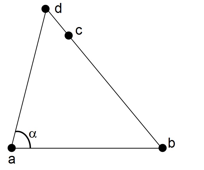
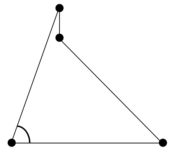
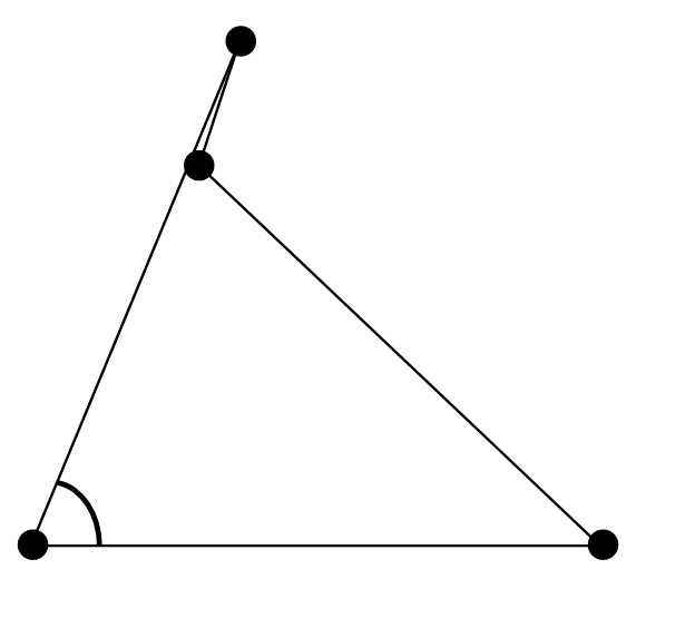
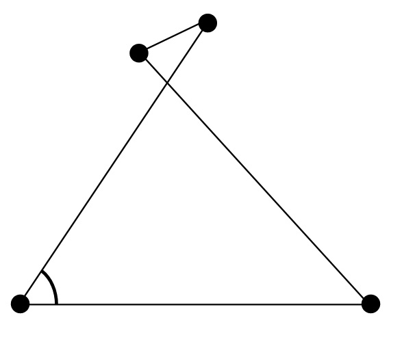
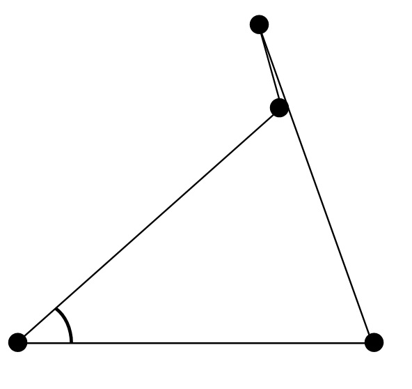
(a)	(b)	(c)	(d)	(e)

Figure 13. A quadrilateral with three long sides

Thus  $\overline{{\mathcal{C}}}^{\operatorname{re}}_{\ast}({\Gamma})$   is homeomorphic to the slit sphere  $\overline{{\mathbf{S}}^{2}\setminus\widehat{\mathbf{g}\mathbf{h}}}$   (including the two edges of the cut), and the full reduced configuration space  $\widehat{{\mathcal{C}}}_{\ast}^{\operatorname{re}}(\Gamma)$   is  $\overline{{\mathbf{S}}^{2}\setminus\widehat{\mathbf{g}\mathbf{h}}}\times{\mathbf{S}}^{1}$.  Finally, the unreduced configuration space is

$$\ \widehat{{\mathcal{C}}}(\Gamma){}\ ~{}\cong~{}\overline{{\mathbf{S}}^{2}\setminus\widehat{\mathbf{g}\mathbf{h}}}~{}\times~{}{\mathbf{S}}^{1}~{}\times~{}{\mathbf{S}}^{2}~{}\times~{}{\mathbb{R}}^{3}~{},$$

since the quadrilateral can never be full aligned.

8.B.    Open chains

For an open chain  $\Gamma^{2}_{\operatorname{op}}$   with two links (cf. §1.4), we have  $\operatorname{Emb}{{\mathcal{T}}_{\Gamma^{2}_{\operatorname{op}}}}=\widehat{\operatorname{Emb}}{{\mathcal{T}}_{\Gamma^{2}_{\operatorname{op}}}}$   and  ${\mathcal{C}}({\Gamma^{2}_{\operatorname{op}}})=\widehat{{\mathcal{C}}}(\Gamma^{2}_{\operatorname{op}})$,  since no self-intersections exist in our model. Moreover,  $\operatorname{Emb}^{\operatorname{re}}_{\ast}({{\mathcal{T}}_{\Gamma^{2}_{\operatorname{op}}}})\cong{\mathbf{S}}^{2}\times(0,\infty)\times(0,\infty)$   and  ${\mathcal{C}}^{\operatorname{re}}_{\ast}({\Gamma^{2}_{\operatorname{op}}})\cong{\mathbf{S}}^{2}$,  and we can choose spherical coordinates  $(\theta,\phi)$   for  ${\mathbf{S}}^{2}$,  where $\theta$ is the rotation of the second edge about the first. The coordinates  $(\ell_{1},\ell_{2})\in(0,\infty)\times(0,\infty)$   are the link lengths.

For an open chain  $\Gamma^{3}_{\operatorname{op}}$   with three links, we first consider the simplified case where the first and third link have infinite length: that is, the linkage  $\widehat{\Gamma}^{3}_{\operatorname{op}}$   has two half-lines $\vec{\mathbf{p}}$ and $\vec{\mathbf{q}}$, whose ends are joined by an interval $I$.

If we do not specify the length of $I$, this linkage type is equivalent to  ${\mathcal{T}}_{\Gamma_{6}}$   of §5.6. The specific mechanism $\Gamma$ with  $|I|=\ell^{2}$   corresponds to choosing the vector $\vec{\mathbf{w}}$ in §5.6 to be of length  $\ell^{2}$,  thus replacing  ${\mathbb{R}}^{3}$   there by a sphere  ${\mathbf{S}}^{2}$,  and replacing $X$ by its two poles $N$ and $S$. Thus we see that

$${\mathcal{C}}^{\operatorname{re}}({\widehat{\Gamma}^{3}_{\operatorname{op}}})~{}\simeq~{}{\mathcal{C}}^{\operatorname{re}}_{\ast}({\widehat{\Gamma}^{3}_{\operatorname{op}}})~{}\simeq~{}{\mathbf{S}}^{2}\vee{\mathbf{S}}^{2}\vee{\mathbf{S}}^{2}~{}.$$

The case where  $\ell_{1}$   is finite and  $\ell_{3}$   is infinite is analogous. When both are finite, we must distinguish the case when  $\ell_{1}+\ell_{3}>\ell_{2}$   (again analogous to the infinite case) from that in which  $\ell_{1}+\ell_{3}\leq\ell_{2}$   (in which case  ${\mathcal{C}}^{\operatorname{re}}_{\ast}({\widehat{\Gamma}^{3}_{\operatorname{op}}})\cong{\mathbf{S}}^{2}\times{\mathbf{S}}^{2}$).

The analysis of open chains with more links requires a more complicated analysis of the moduli space of link lengths (see below).

9. Appendix:  Spaces of paths

There is yet another construction which can be used to describe the virtual configurations of a linkage $\Gamma$, which we include for completeness, even though it is not used in this paper.

9.1 Definition.

Given a linkage type  ${\mathcal{T}}_{\Gamma}$   with  $\operatorname{Emb}({\mathcal{T}}_{\Gamma})\subseteq({\mathbb{R}}^{3})^{V}$,  let  $P({\mathcal{T}}_{\Gamma})$   denote the space of paths  $\gamma:[0,1]\to({\mathbb{R}}^{3})^{V}$   such that  $\gamma((0,1])\subseteq\operatorname{Emb}({\mathcal{T}}_{\Gamma})$   (cf. [L, Ch. 3]), and let  $\operatorname{ev}_{0}:P({\mathcal{T}}_{\Gamma})\to({\mathbb{R}}^{3})^{V}$   send  $[\gamma]$   to  $\gamma(0)$.  Let  $E({\mathcal{T}}_{\Gamma})$   denote the set of homotopy classes of such paths relative to  $\mathbf{x}=\gamma(0)$.  This is a quotient space of  $P({\mathcal{T}}_{\Gamma})$,  with  $\widehat{\operatorname{ev}}_{0}:E({\mathcal{T}}_{\Gamma})\to({\mathbb{R}}^{3})^{V}$   induced by  $\operatorname{ev}_{0}$.  We shall call  $E({\mathcal{T}}_{\Gamma})$   the path space of embeddings of  ${\mathcal{T}}_{\Gamma}$.

Similarly, let  $P(\Gamma)\subseteq P({\mathcal{T}}_{\Gamma})$   denote the space of paths  $\gamma:[0,1]\to({\mathbb{R}}^{3})^{V}$   such that  $\gamma((0,1])\subseteq{\mathcal{C}}({\Gamma})$,  with  $E(\Gamma)$   the corresponding set of relative homotopy classes (a quotient of  $P(\Gamma)$).  We call  $E(\Gamma)$   the path space of configurations of $\Gamma$.

9.2 Lemma.

The completed space of embeddings  $\widehat{\operatorname{Emb}}({\mathcal{T}}_{\Gamma})$   is a quotient of the path space  $E({\mathcal{T}}_{\Gamma})$,  and  $\widehat{{\mathcal{C}}}(\Gamma)$   is a quotient of  $E(\Gamma)$.

Proof.

First note that when  $\gamma(0)\in\operatorname{Emb}({\mathcal{T}}_{\Gamma})$,  the path $\gamma$ is completely contained in the open subspace  $\operatorname{Emb}({\mathcal{T}}_{\Gamma})$   of  $({\mathbb{R}}^{3})^{V}$,  so we may represent any homotopy  $[\gamma]$   by a path contained wholly in an open ball around  $\gamma(0)$   inside  $\operatorname{Emb}({\mathcal{T}}_{\Gamma})$,  and any two such paths are linearly homotopic. Thus  $\widehat{\operatorname{ev}}_{0}$   restricted to  $\operatorname{Emb}({\mathcal{T}}_{\Gamma}))$   is a homeomorphism.

In any completion $\hat{X}$ of a metric space  $(X,d)$,  the new points can be thought of as equivalence classes of Cauchy sequences in $X$. Since we can extract a Cauchy sequence (in the path metric) from any path $\gamma$ as above, and homotopic paths have equivalent Cauchy sequences, this defines a continuous map  $\phi:E({\mathcal{T}}_{\Gamma})\to\widehat{\operatorname{Emb}}({\mathcal{T}}_{\Gamma})$.

In our case,  $X=\operatorname{Emb}({\mathcal{T}}_{\Gamma})$   also has the structure of a manifold, and given any Cauchy sequence  $(x_{i})_{i=1}^{\infty}$   in $X$, choose an increasing sequence of integers  $n_{k}$   such that  $d_{\operatorname{path}}(x_{i},x_{j})<2^{-k}$   for all  $i,j\geq n_{k}$.  By definition of  $d_{\operatorname{path}}$,  we have a path  $\gamma^{k}$   from  $x_{n_{k}}$   to  $x_{n_{k+1}}$   of length  $\leq 2^{-k}$.  By concatenating these and using Remark 2.2, we obtain a smooth path $\gamma$ along which all  $(x_{i})_{i=1}^{\infty}$   lies. Thus we may restrict attention to Cauchy sequences  $(x_{i})_{i=1}^{\infty}=(\gamma(t_{i}))_{i=1}^{\infty}$   lying on a smooth path $\gamma$ in $X$. We can parameterize $\gamma$ so that  $\gamma((0,1])\subseteq\operatorname{Emb}({\mathcal{T}}_{\Gamma})$,  and let  $\gamma(0):=\lim_{i\to\infty}\,x_{i}\in({\mathbb{R}}^{3})^{V}$,  which exists since  $({\mathbb{R}}^{3})^{V}$   is complete. Thus $\phi$ is surjective. ∎

We may thus summarize the constructions in this paper in the following diagram, generalizing  (3.7)  :

(9.3)

Similarly for the various types of configuration spaces shown in  (3.8).

9.4 Remark.

If we allow a linkage type  ${\mathcal{T}}={\mathcal{T}}_{\Gamma_{\infty}}$   consisting of a countable number of lines, we show that the maps  $\phi:E({\mathcal{T}}_{\Gamma})\to\widehat{\operatorname{Emb}}({\mathcal{T}}_{\Gamma})$   and  $\phi:E(\Gamma)\to\widehat{{\mathcal{C}}}(\Gamma)$   need not be one-to-one, in general:

Consider the set $S$ of configurations $\mathbf{x}$ of ${\mathcal{T}}$ in which the first line  $\mathbf{x}(\ell_{0})$   is the $x$-axis in  ${\mathbb{R}}^{3}$,  and all other lines  $\mathbf{x}(\ell_{n})$    ($n=1,2,\dotsc$)   are perpendicular to the  ($x,y$)-plane, and thus determined by their intersections  $\mathbf{z}(\ell_{n})$   with the  ($x,y$)-plane, with  $\mathbf{z}(\ell_{n})=(0,1/n)$   for  $n\geq 2$.  Thus the various configurations in $S$ differ only in the location of  $\mathbf{z}(\ell_{1})$.

Now define the following two Cauchy sequences  $(\mathbf{x}^{\prime}_{k})_{k=1}^{\infty}$   and  $(\mathbf{x}^{\prime\prime}_{k})_{k=1}^{\infty}$   in  $S\subseteq\operatorname{Emb}({\mathcal{T}}_{\Gamma_{\infty}})={\mathcal{C}}(\Gamma_{\infty})$:  we let  $\mathbf{z}^{\prime}_{k}(\ell_{1}):=(1/k,1/k)$   for  $\mathbf{x}^{\prime}_{k}$,  while  $\mathbf{z}^{\prime\prime}_{k}(\ell_{1}):=(-1/k,1/k)$   for  $\mathbf{x}^{\prime\prime}_{k}$.  Since we can define a path in $S$ between  $\mathbf{x}^{\prime}_{k}$   and  $\mathbf{x}^{\prime\prime}_{k}$   of length $<3/k$, the two Cauchy sequences are equivalent, and thus define the same point in the completions  $\widehat{\operatorname{Emb}}({\mathcal{T}}_{\Gamma_{\infty}})=\widehat{{\mathcal{C}}}(\Gamma_{\infty})$.  However, if we embed  $(\mathbf{x}^{\prime}_{k})_{k=1}^{\infty}$   in a path  $\gamma^{\prime}:[0,1]\to S$   defined by the intersection  $\mathbf{z}^{\prime}_{t}(\ell_{1}):=(t,t)$,  and similarly for  $(\mathbf{x}^{\prime\prime}_{k})_{k=1}^{\infty}$,  it is easy to see that  $\gamma^{\prime}$   and  $\gamma^{\prime\prime}$   cannot be homotopic (relative to endpoints), so they define different points in  $E({\mathcal{T}}_{\Gamma})$   or  $E(\Gamma)$.

References

- [CEGSS] B. Chazelle, H. Edelsbruner, K.J. Guibas, M. Sharir, & J. Stolfi, “Lines in Space: Combinatorics and Algorithms”, Algorithmica 15 (1996), pp. 428-447.
- [CP] H. Crapo & R.J. Penne, “Chirality and the isotopy classification of skew lines in projective -space”, Adv. Math. 103 (1994), pp. 1-106.
- [CF] R.H. Crowell & R.H. Fox”, Introduction to Knot Theory, Springer, Berlin-New York, 1963.
- [DV] Yu.V. Drobotukhina & O.Ya. Viro, “ Configurations of skew-lines”, Algebra i Analiz1 (1989), pp. 222-246.
- [Fa] M.S. Farber, Invitation to Topological Robotics, European Mathematical Society, Zurich, 2008.
- [FTY] M.Š. Farber, S. Tabachnikov, & S.A. Yuzvinskiĭ, “Topological robotics: motion planning in projective spaces”, Int. Math. Res. Notices 34 (2003), 1853-1870.
- [Fr] A. Friedman, Foundations of Modern Analysis, Dover, New York, 1970.
- [G] D.H. Gottlieb, “Robots and fibre bundles”, Bull. Soc. Math. Belg. Sér. A 38 (1986), 219-223.
- [Hal] A.S. Hall, Jr., Kinematics and Linkage Design, Prentice-Hall, Englewood Cliffs, NJ, 1961.
- [Hau] J.-C. Hausmann, “Sur la topologie des bras articulés”, in S. Jackowski, R. Oliver, & K. Pawałowski, eds., Algebraic Topology - Poznán 1989, Lect. Notes Math. 1474, Springer Verlag, Berlin-New-York, 1991, pp. 146-159.
- [HK] J.-C. Hausmann & A. Knutson, “The cohomology ring of polygon spaces”, Ann. Inst. Fourier (Grenoble) 48 (1998), pp. 281-321.
- [Ho] M. Holcomb, “On the Moduli Space of Multipolygonal Linkages in the Plane”, Topology & Applic. 154 (2007), pp. 124-143.
- [JS] D. Jordan & M. Steiner, “Compact surfaces as configuration spaces of mechanical linkages”, Israel J. Math. 122 (2001), pp. 175-187.
- [KM1] M. Kapovich & J. Millson, “On the moduli space of polygons in the Euclidian plane”, J. Diff. Geom. 42 (1995), pp. 430-464.
- [KM2] M. Kapovich & J. Millson, “The symplectic geometry of polygons in Euclidean space”, J. Diff. Geom. 44 (1996), pp. 479ג513.
- [K] Y. Kamiyama, “Topology of equilateral polygon linkages in the Euclidean plane modulo isometry group”, Osaka J. Math. 36 (1999), pp. 731-745.
- [KT] Y. Kamiyama & S. Tsukuda, “The configuration space of the -arms machine in the Euclidean space”, Topology & Applic. 154 (2007), pp. 1447-1464.
- [L] J.M. Lee, Riemannian manifolds. An introduction to curvature, Springer-Verlag, Berlin-New York, 1997.
- [Me] J. P. Merlet, Parallel Robots, Kluwer Academic Publishers, Dordrecht, 2000.
- [MT] R.J. Milgram & J. Trinkle, “The Geometry of Configuration spaces of Closed Chains in Two and Three Dimensions”, Homology, Homotopy & Applic. 6 (2004), pp. 237-267.
- [Mu] J.R. Munkres, Topology, A First Course, Prentice-Hall, Englewood, NJ, 1975.
- [OH] J. O’Hara, “The configuration space of planar spidery linkages”, Topology & Applic. 154 (2007), pp. 502-526.
- [P] R.J. Penne, “Configurations of few lines in -space: Isotopy, chirality and planar layouts”, Geom. Dedicata 45 (1993), pp. 49 82.
- [RR] G. Rodnay & E. Rimon, “Isometric visualization of configuration spaces of two-degrees-of-freedom mechanisms”, Mechanism and machine theory 36 (2001), pp. 523-545.
- [Se] J.M. Selig, Geometric Fundamentals of Robotics, Springer-Verlag Mono. Comp. Sci., Berlin-New York, 2005.
- [Sh] I.R. Shafarevich, Basic algebraic geometry, 1. Varieties in projective space, Springer-Verlag, Berlin-New York, 1994.
- [SSB] N. Shvalb, M. Shoham & D. Blanc, “The Configuration Space of Arachnoid Mechanisms”, Fund. Math. 17 (2005), 1033-1042.
- [T] L.W. Tsai, Robot Analysis - The mechanics of serial and parallel manipulators, Wiley interscience Publication - John Wiley & Sons, New York, 1999.
- [Va] V.A. Vassiliev, “Knot invariants and singularity theory”, in Singularity theory (Trieste, 1991), World Sci. Publ., River Edge, NJ, 1995, pp. 904-919.
- [Vi] O.Ya. Viro, “Topological problems on lines and points of three-dimensional space”, Dokl. Akad. Nauk SSSR 284 (1985), pp. 1049 1052.