Single and double linear and nonlinear flatband chains: spectra and modes

Abstract

We report results of systematic analysis of various modes in the flatband lattice, based on the diamond-chain model with the on-site cubic nonlinearity, and its double version with the linear on-site mixing between the two lattice fields. In the single-chain system, a full analysis is presented, first, for the single nonlinear cell, making it possible to find all stationary states, viz., antisymmetric, symmetric, and asymmetric ones, including an exactly investigated symmetry-breaking bifurcation of the subcritical type. In the nonlinear infinite single-component chain, compact localized states (CLSs) are found in an exact form too, as an extension of known compact eigenstates of the linear diamond chain. Their stability is studied by means of analytical and numerical methods, revealing a nontrivial stability boundary. In addition to the CLSs, various species of extended states and exponentially localized lattice solitons of symmetric and asymmetric types are studied too, by means of numerical calculations and variational approximation. As a result, existence and stability areas are identified for these modes. Finally, the linear version of the double diamond chain is solved in an exact form, producing two split flatbands in the system’s spectrum.

I Introduction

The behavior of dynamical lattices, which model a vast variety of physical systems, is determined by the interplay of their linear-excitation spectra and local nonlinearity Moti -Jena . An essential peculiarity of many lattices is the presence of at least one flatband (FB), i.e., a dispersionless branch in the spectrum richter . Interest to FBs was drawn by their discovery in the Hubbard Tasaki and Su-Schrieffer-Heeger models, where they underlie the existence of a stable ferromagnetic phase. It was also demonstrated that the FB may cause insulator-metal transitions in the underlying lattices transition . Further, quantum-Hall and topological-insulator states were predicted in FB systems Hall . Lattices can support FBs in diverse physical settings, including arrayed optical waveguides diamond ; guzman-silva14 , exciton-polariton condensates in semiconductor microcavities with lattice patterns etched into them masumoto12 ; cavities , and atomic Bose-Einstein condensates (BECs) loaded into an appropriately designed optical lattice ZhangZhang ; taie15 .

A remarkable property of linear dynamical lattices featuring the FB spectrum is that, in addition to the usual dispersive “phonon” excitations, they support exact eigenmodes in the form of compact localized states (CLSs), which include a finite number of lattice sites with nonzero amplitudes richter ; flach14 ; add1 . In particular, these states may be robust against the presence of disorder in the system disorder . A local resonant mechanism, which is similar to the Fano resonance miroshnichenko10 , may hybridize the CLS with the phonon modes, thus giving rise to new varieties of lattice excitations flach14 . Experimentally, the existence of CLSs has been demonstrated in the above-mentioned settings which admit the realization of the FB spectra, viz., optical waveguiding arrays vicencio15 ; add2 ; add3 ; mukherjee15 ; weimann16 , exciton-polariton condensates cavities , and atomic BECs taie15 .

Unlike the self-trapped discrete solitons in nonlinear lattices Moti -Jena , the localization of CLSs does not require the presence of nonlinearity. On the other hand, nonlinearities, represented by the Kerr term in optics and collisional term in BEC, are naturally present in physical settings which admit the realization of FBs and CLSs. This fact suggests to explore the existence and dynamics of CLSs in nonlinear lattices, and their possible relations to exponentially localized (but not compact) discrete solitons, which are generic modes in nonlinear lattices. In recent works, it was demonstrated that the nonlinearity may produce various effects in FB systems, such as stabilization or destabilization of the compact states, detuning of their frequencies, interactions between CLSs, and coexistence and interactions between CLSs and lattice solitons vicencio13 ; add4 ; flach14 ; johannson15 ; lopez-gonzalez16 ; Sandra ; Maimistov .

The purpose of this paper is two-fold. First, we aim to develop a nonlinear version of the FB system based on the known configuration in the form of the “diamond chain” flach14 (see Fig. 1), by adding the on-site cubic nonlinearity to it. Working in this direction, we aim to construct CLSs and usual (exponentially localized, but not compact) discrete solitons in this chain, and analyze their stability. Results obtained for the CLSs demonstrate specific extension of this type of modes into the realm of the nonlinearity: they keep to exists as compact states, featuring a nontrivial stability boundary inside their family, which is a manifestation of the nonlinearity. Stability boundaries for families of exponentially localized discrete solitons are found too. Second, we introduce a double diamond chain, with on-site linear coupling between two components. It can also be readily implemented in optics, considering arrays of double-core waveguides Christo , and in BEC, as a binary condensate whose components are Rabi-coupled by a resonant electromagnetic field binary .

Analytical results for the nonlinear one-chain model are reported in Section II. They present a full exact solution for the single nonlinear diamond cell (rather than in the chain), including both symmetric and asymmetric states, and an exact solution for the CLS in the infinite nonlinear chain, including a partial analysis of its stability. Numerical findings for the single nonlinear chain are presented in Section III. These include extended modes, which may be considered as fragments of continuous-wave (CW) states, symmetric and asymmetric exponentially localized lattice solitons, and the full analysis of the stability of the nonlinear CLS. Further, in Section V we present analytical results for the lattice solitons in the nonlinear chain, obtained by means of the variational approximation (VA), which compare well to their numerical counterparts. Finally, section VI concludes the paper.

II The single-component model: analytical results

II.1 The formulation

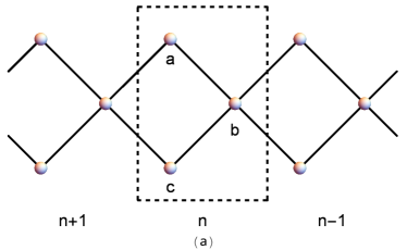
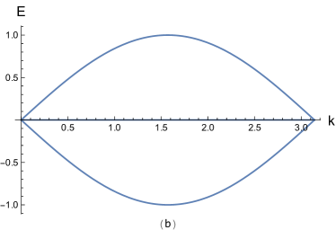
Figure 1: (a) The single-component diamond chain. (b) The respective dispersion relation.

We consider the quasi-1D lattice in the form of the “diamond chain” with the on-site cubic nonlinearity, which is shown in Fig. 1(a). The band structure of the chain’s linear version, plotted in Fig. 1(b), is produced by Eq. (8), see below. The spectrum contains two dispersive bands which intersect with the third, flat band, at edges of the Brillouin zone. The intersections create Dirac points with conical dispersion around them.

The dynamics of the diamond lattice is governed by equations for complex amplitudes at sites labeled $a$, $b$, and $c$ in Fig. 1(a):

$$i\frac{da_{n}}{dz}+(b_{n}+b_{n+1})+\beta|a_{n}|^{2}a_{n}=0,$$

$$i\frac{db_{n}}{dz}+(a_{n}+a_{n-1}+c_{n}+c_{n-1})+\beta|b_{n}|^{2}b_{n}=0,$$ (1)

$$i\frac{dc_{n}}{dz}+(b_{n}+b_{n+1})+\beta|c_{n}|^{2}c_{n}=0.$$

Here evolution variable $z$ is the propagation distance, if the lattice is realized as an array of optical waveguides diamond ; guzman-silva14 ; vicencio15 ; add2 ; add3 ; mukherjee15 ; weimann16 , $n$ is the cell’s number in the chain, the inter-site coupling constant is scaled to be $1$, and $\beta$ is the strength of the on-site nonlinearity. The propagation equations can be derived from the corresponding Hamiltonian,

$$\mathcal{H}=\sum_{n}\big{(}[(a_{n}^{\ast}+c_{n}^{\ast})(b_{n}+b_{n+1})+\mathrm{c.c.}]$$

$$+\frac{\beta}{2}(|a_{n}|^{4}+|b_{n}|^{4}+|c_{n}|^{4})]\big{)},$$ (2)

where both the asterisk and $\mathrm{c.c.}$ stand for the complex-conjugate expression. The Hamiltonian is a dynamical invariant of system (1), along with the total norm,

$$N=\sum_{n}(|a_{n}|^{2}+|b_{n}|^{2}+|c_{n}|^{2}).$$ (3)

Here we assume that $\beta$ is positive. Then, using the scaling invariance of the system, one can fix $\beta=1$, while $N$ will play the role of a parameter of families of stationary states (in the analytical part of the work, we do not fix $\beta=1$, since keeping $\beta>0$ as a free coefficient does not make analytical results cumbersome). In Eqs. (17) with $\beta<0$, the sign of the nonlinearity coefficient can be reversed by changing $b_{n}\rightarrow-b_{n}$ and replacing the equations by their complex-conjugate version.

Eigenmodes of system (1) with real propagation constant $E$ are looked for as

$$\{{a}_{n}(z),{b}_{n}(z),{c}_{n}(z)\}=\left\{A_{n},B_{n},C_{n}\right\}e^{iEz},$$ (4)

with stationary amplitudes $\left\{A_{n},B_{n},C_{n}\right\}$ satisfying the following equations:

$$-EA_{n}+(B_{n}+B_{n+1})+\beta|A_{n}|^{2}A_{n} =0,$$ (5)

$$-EB_{n}+(A_{n}+A_{n-1}+C_{n}+C_{n-1})+\beta|B_{n}|^{2}B_{n} =0,$$ (6)

$$-EC_{n}+(B_{n}+B_{n+1})+\beta|C_{n}|^{2}C_{n} =0.$$ (7)

The spectrum of the linearized version of (5)-(7) contains three branches,

$$E(k)=0,~{}\pm 2\sqrt{2}\cos(k/2),$$ (8)

which are shown above in Fig. 1(b). Obviously, $E(k)=0$ represents the FB. The branches were derived by substituting, in the linearized equations, the continuous-wave (CW) ansatz, $\left\{A_{n},B_{n},C_{n}\right\}=\left\{A,B,C\right\}e^{ikn}$, with real wavenumber $k$ which takes values in the first Brillouin zone, $-\pi\leq k\leq+\pi$. The eigenmodes corresponding to the flat (“0”) and dispersive (“$\pm$”) branches (8) amount, respectively, to the following sets of constant amplitudes:

$$\left\{A,B,C\right\}_{0}=\frac{1}{\sqrt{2}}(1,0,-1),\,\left\{A,B,C\right\}_{\pm}=\frac{1}{2}(1,\pm\sqrt{2}e^{-ik/2},1).$$ (9)

The CLSs are produced by the exact solution in the form of Eq. (4) with $E=0$ (and zero group velocity), which is completely localized in a single unit cell, centered at an arbitrary position, $n=N_{0}$:

$$\left\{A_{n},B_{n},C_{n}\right\}=\frac{1}{\sqrt{2}}\delta_{n,N_{0}}(1,0,-1),$$ (10)

where $\delta_{m,n}$ is the Kronecker’s symbol richter ; flach14 . This solution exists due to the destructive interference (cancellation of the field) at site $b$ [see Fig. 1(a)], which is provided by the $\pi$ phase difference between the $a$ and $c$ sites. In contrast, eigenmodes (9) corresponding to the dispersive bands are completely delocalized plane waves. Because CLSs are degenerate modes in the linear system, with respect to their placement in the lattice, their arbitrary combinations are exact solutions too vicencio15 ; add1 ; add2 . In this way, one can easily construct extended states (fragments of CWs) localized on several adjacent cells of the lattice.

As mentioned above, experimental realization of flat bands and CLSs was reported in Refs. vicencio15 ; mukherjee15 ; weimann16 , while counterparts of CLSs in nonlinear lattices were discussed in Refs. vicencio13 ; flach14 ; johannson15 ; lopez-gonzalez16 ; Sandra ; add4 . In this work, we aim to develop the analysis of CLSs and lattice solitons coexisting with them in the nonlinear diamond-chain system.

II.2 Reduced problem: one cell of the single nonlinear chain

II.2.1 The setting

We begin the analysis of the nonlinear diamond chain by consideration of the simplest case of the system truncated to a single cell, which is drawn in Fig. 2. It contains single “A” and “C” sites, which communicate to each other via two “B” sites (the structure of the system implies that two fields at the B sited are identical).

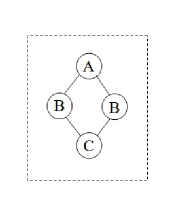
Figure 2: The truncated single-cell nonlinear system.

The truncated system is based on the following system of equations, in which the on-site nonlinearity coefficient is scaled to be $\beta\equiv 1$ (if $\beta$ is negative, its sign can be inverted by means of a simple transformation, $b\rightarrow-b,$ $z\rightarrow-z$):

$$i\frac{da}{dz}+2b+|a|^{2}a=0,$$ (11)

$$i\frac{dc}{dz}+2b+|c|^{2}c=0.$$ (12)

$$i\frac{db}{dz}+a+c+|b|^{2}b=0,$$ (13)

This system with three degrees of freedom conserves two dynamical invariants: the Hamiltonian,

$$H=\frac{1}{2}\left(|a|^{4}+|c|^{4}+2|b|^{4}\right)+2[b(a^{\ast}+c^{\ast})+b^{\ast}(a+c)]$$ (14)

cf. Eq. (2), and the norm,

$$N=|a|^{2}+|c|^{2}+2|b|^{2},$$ (15)

cf. Eq. (3). The Hamiltonian representation of Eqs. (11)-(13) (i.e., the corresponding Poisson brackets/symplectic structure) is based on equations

$$\frac{da}{dz}=i\frac{\partial H}{\partial a^{\ast}},~{}\frac{dc}{dz}=i\frac{\partial H}{\partial c^{\ast}},~{}\frac{db}{dz}=\frac{i}{2}\frac{\partial H}{\partial b^{\ast}}.$$ (16)

Although the present model with three degrees of freedom seems very simple, to the best of our knowledge it was not explored before. Below, we report a full analysis of exact stationary solutions of this system and their stability, which can be easily realized in the experiment.

II.2.2 Antisymmetric and symmetric stationary solutions

Stationary solutions to Eqs. (11)-(13) with a real propagation constant, $E$, are looked for as

$$\{{a}(z),{b}(z),{c}(z)\}=\left\{A,B,C\right\}e^{iEz},$$ (17)

cf. Eq. (4), with amplitudes $\left\{A,B,C\right\}$ determined by the algebraic equations:

$$-EA+2B+A^{3} = 0,$$ (18a)

$$-EC+2B+C^{3} = 0,$$ (18b)

$$-EB+A+C+B^{3} = 0.$$ (18c)

These equations have an obvious antisymmetric solution,

$$B=0,~{}A=-C=\sqrt{E},$$ (19)

which exists at $E\geq 0$ (all the solutions can be defined as those with $A>0$; obviously, there is also a solution with opposite signs in front of all the amplitudes).

There are also symmetric solutions, with $A=C$, $B\neq 0$. Four different solutions of this type can be identified. The first is

$$A=C=B=\sqrt{E-2},$$ (20)

which exists at $E\geq 2$, and there is another solution, with

$$A=C=-B=\sqrt{E+2},$$ (21)

which exists at $E\geq-2$. Finally, there are two additional symmetric solutions, which correspond to signs $\pm$ in Eq. (22), and exist at $E\geq 4$:

$$A=C=\sqrt{\frac{1}{2}\left(E\pm\sqrt{E^{2}-16}\right)},~{}B=\frac{2}{A}\equiv\sqrt{\frac{1}{2}\left(E\mp\sqrt{E^{2}-16}\right)}.$$ (22)

II.2.3 Bifurcation points

The symmetric solutions undergo a symmetry-breaking bifurcation (SBB), which gives rise to nontrivial asymmetric solutions, with $A\neq C$. The analysis of the transition from symmetric states to asymmetric ones is an issue of general interest book0 ; book , including the present model. Bifurcation points (there are two such critical points) can be found analytically. To this end, replacing Eqs. (18a) and (18b) by their sum and difference, and canceling in the latter one a common factor, $A-C\neq 0$, the system of algebraic equations (18a)-(18c) is replaced by the following one:

$$E=A^{2}+C^{2}+AC,$$ (23a)

$$-E\left(A+C\right)+4B+A^{3}+C^{3}=0,$$ (23b)

$$-EB+A+C+B^{3}=0.$$ (23c)

Exactly at the SBB point, Eqs. (23a)-(23b) must have a solution with $$A=C$$. It is easy to find that this is possible at two points (as mentioned above):

$$E=3,~{}A=C=B=1,$$ (24)

and

$$E=3\sqrt{2},~{}A=C=2^{1/4},~{}B=2^{3/4}.$$ (25)

Obviously, the bifurcation point (24) pertains to symmetric solution (20), while point (25) pertains to symmetric solution (22) with sign minus chosen for $\pm$.

The similar analysis for the antisymmetric solution readily demonstrates that it never undergoes an antisymmetry-breaking bifurcation (formally, the bifurcation occurs at an unphysical point, with $E^{2}=-2$).

II.2.4 The analysis of the bifurcations

To identify the character of the SBB at point (24), we consider solutions of Eqs. (23a)-(23c) in an infinitesimal vicinity of the bifurcation, setting

$$E = 3-\epsilon,~{}0<\epsilon\ll 1,$$ (26)

$$A = 1-\alpha\epsilon+\gamma\sqrt{\epsilon},$$ (27)

$$C = 1-\alpha\epsilon-\gamma\sqrt{\epsilon},$$ (28)

$$B = 1-\beta\epsilon.$$ (29)

In Eq. (26), term $\sim\epsilon$ is defined with sign minus in front of it in the anticipation of the fact that the SBB will be subcritical book0 at this point. The substitution of Eqs. (26)-(29) into Eqs. (23a)-(23c) and expanding the result up to order $\epsilon$ easily yields the following results:

$$\gamma^{2} = 2,$$ (30)

$$\alpha = 1/2,~{}\beta=7/2$$ (31)

The conclusion is that the SBB at point (24) is indeed subcritical: the asymmetric solutions originally move backward (in the direction of decreasing $E$), as unstable ones, after emerging at the bifurcation point. Later, they turn forward, passing the respective turning point, where they undergo stabilization book0 .

Furthermore, it is relevant to check if Eqs. (23a)-(23c) would admit a regular extension of the solutions from point (24) (i.e., built in terms of $\epsilon$, rather than $\sqrt{\epsilon}$), instead of the bifurcation. This implies looking for a solution in the form of the following expansion, instead of Eqs. (27)-(29):

$$A=1-a\epsilon,~{}C=1-c\epsilon,~{}B=1-b\epsilon.$$ (32)

Then, the substitution of this into Eq. (23a) yields $a+c=1/3$, while the substitution into Eq. (23c) yields $a+c=1$. This contradiction implies that regular expansion (32) cannot produce a solution, the bifurcation being the only possibility.

Similarly, in a vicinity of bifurcation point (25) we seek for a solution to Eqs. (23a)-(23c) in the form of

$$E = 3\sqrt{2}-\epsilon,~{}|\epsilon|\ll 1,$$ (33)

$$A = 2^{1/4}-\alpha\epsilon+\gamma\sqrt{\epsilon},$$ (34)

$$C = 2^{1/4}-\alpha\epsilon-\gamma\sqrt{\epsilon},$$ (35)

$$B = 2^{3/4}-\beta\epsilon.$$ (36)

The same procedure as the one outlined above for the SBB at point (24) yields $\gamma^{2}=-1/7,$ $\alpha=(1/7)\cdot 2^{-1/4},$ $\beta=(4/7)\cdot 2^{-3/4}$. The formal result with $\gamma^{2}<0$ means that the bifurcation at point (25) actually does not take place. Thus, the actual SBB takes place solely at point (24).

II.2.5 Asymmetric solutions

The asymmetric solutions produced by the SBB can be easily found in the asymptotic form at $E\rightarrow+\infty$ directly from Eqs. (18a)-(18b):

$$A\approx\sqrt{E},~{}B\approx A/E\approx 1/\sqrt{E},~{}C\approx 2B/E\approx 2/E^{3/2}.$$ (37)

The existence of the single solution in the asymptotic form (37) agrees with the conclusion made in the previous subsection, where it was found that only one bifurcation point, given  by Eq. (24), is a real one. In the general case, the asymmetry  of the solutions is defined by

$$\Theta\equiv\frac{A^{2}-C^{2}}{A^{2}+C^{2}}.$$ (38)

Next, we aim to address asymmetric solutions emerging from the point of the subcritical SBB. The system of three coupled cubic algebraic equations (18a), (18c) and (18b) has 27 roots, which makes it impossible to present them in an explicit analytical form. Most roots are complex, hence they are unphysical. One root remains real at $E>3$, i.e., above the SBB point (24). This solution describes the stable part of the asymmetric-solution branch where it goes forward, after passing the turning point (see the continuous lines in Fig. 3). On the other hand, there also exists another solution which remains real in a very narrow range: $2.994\lesssim E\leq 3$. It represents the initial short backward-going unstable segment of the asymmetric branch, which is shown by dashed lines in Fig. 3.

Figure 3: The bifurcation diagram for the weakly subcritical transition from symmetric to asymmetric stationary states in the nonlinear single-cell system. The asymmetry parameter, defined as per Eq. (38), is shown versus propagation constant $E$ of the stationary solutions. Stable and unstable branches of asymmetric solutions are shown by solid and dashed curves, respectively.

II.3 The single infinite chain: nonlinear compact localized states (CLSs) and their stability

Some simple but essential analytical results can be obtained also for the infinite diamond chain based on nonlinear equations (1) and (5), (7), (6) (here, we keep the nonlinearity coefficient $\beta$ as a free parameter). It admits an obvious solution for $E>0$, which is a nonlinear extension of the CLS (10) obtained for $E=0$ in the linear lattice:

$$A_{0}=-C_{0}=\sqrt{E/\beta},~{}\mathrm{all~{}~{}other}~{}A_{n},C_{n},B_{n}=0$$ (39)

[cf. an equivalent single-cell state given by Eq. (19)]. It is relevant to consider, in an analytical form, the stability of this exact antisymmetric solution (with $A_{0}=-C_{0}$) against antisymmetry-breaking perturbations, or, in other words, a possibility of a bifurcation breaking the antisymmetric form of this state (recall that such a bifurcation does not occur in the single-cell system, as shown above).

To this end, we consider a small perturbation in an originally empty semi-infinite lattice, starting from cite $b_{0}$ at $n=0$, which is followed by sites $a_{0}$ and $c_{0}$ and then by the lattice at sites with $n\geq 1$. If the respective field is $B$ at $n=0$, the solution of linearized equations Eqs. (5), (7), (6) at $n\geq 1$, which is localized, exponentially decaying at $n\rightarrow\infty$, can be easily found:

$$B_{n} = Be^{-\lambda n},~{}A_{n}=C_{n}=\alpha Be^{-\lambda n},$$ (40)

$$\alpha = \frac{1}{4}\left(E-\sqrt{E^{2}-8}\right),$$ (41)

$$e^{-\lambda} = \frac{4}{E^{2}-4+E\sqrt{E^{2}-8}}<1.$$ (42)

This solution exists for $E>\sqrt{8}$.

Then, taking into account the coupling of the two sites $b_{0}$ to the semi-infinite chains originating from them, and to amplitudes $A$ and $C$ at adjacent sites belonging to the cell at $n=0$, Eqs. (6) and (23b) yield

$$\left(A+C\right)+2\alpha B+B^{3} = EB.$$ (43)

$$\left(A^{2}+C^{2}-AC-E\right)\left(A+C\right) = -4B$$ (44)

Finally, the linearization of Eqs. (43) and (44) for small antisymmetry-breaking perturbations, $\left(A+C\right)$ and $B$, leads to the condition for the onset of the respective instability:

$$E^{2}+E\sqrt{E^{2}-8}+4=0.$$ (45)

An elementary consideration of Eq. (45) demonstrates that its only solution is an unphysical one, $E^{2}=-1$ (recall in the single-cell model the analysis has predicted the formal antisymmetry-breaking bifurcation at another unphysical point, $E^{2}=-2$). Thus, the nonlinear CLS (39) is stable against the antisymmetry-breaking perturbations. However, in a part of their parameter space these modes may be destabilized by other perturbations, as shown below.

III The nonlinear infinite single chain: numerical results

All the stationary solutions described below were constructed by means of the imaginary-time method, or applying the Newton-Raphson method for the corresponding nonlinear boundary-value problem. The stability of the solutions was identified by the analysis of linearized equations for small perturbations, and using the linear Cranck-Nicholson scheme for the calculation of the respective eigenvalues. The so predicted stability/instability was then verified through direct simulations of the propagation of initially perturbed modes, utilizing the Crank-Nicholson finite-difference algorithm. In plots presented below, stable and unstable solutions are indicated by continuous and dashed curves, respectively. All the results reported below refer to $\beta=1$, fixed by means of rescaling.

III.1 Continuous-wave (CW) solutions

First, we have examined the existence and stability of CW solutions for the system based on Eqs. (1) and (5)-(7). Diagrams which show amplitudes $A$, $B$ and $C$ as functions of propagation constant $E$, for symmetric, antisymmetric and asymmetric CW states, are presented in Figs. 4, 5 and 6.

For the symmetric case, with $A=C$, three CW families were identified. The first one, which exists for all $E>0$, and is completely stable against modulational perturbations, is shown in Fig. 4. The second family, which is present at $E>9.70$ and features two coexisting branches (Fig. 4), is entirely unstable.The third family, presented in Fig. 4, exists at $E>2.82$ and is totally unstable too (although close to the lower edge – namely, at $2.82<E<2.90$ – the modulational instability of the CW is weak). Direct simulations (not shown here in detail) demonstrate that unstable CWs are transformed into chaotic spatiotemporal states.

Figure 5 introduces antisymmetric CW solutions, with $A=-C$ and $B=0$. It is found to be partially stable – namely, at $E>5.64$, which corresponds to $A=-C>2.38$. In fact, the antisymmetric CW is a limit (delocalized) form of compact antisymmetric solutions, which are presented below in Section III.2.

Two families of asymmetric CWs were found too, both exhibiting two distinct branches, meeting at $E=5.66$. In the case of the asymmetric CW family shown in Fig. 6, a stability region is $E>13.95$, $A>3.99$, $B<-3.96$, and $C>-0.58$.On the other hand, the family of asymmetric CWs displayed in Fig. 6 is completely unstable.

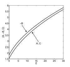
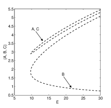
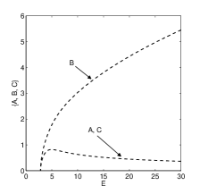
Figure 4: Amplitudes of symmetric CW states versus $E$. Panel (a) displays the stable CW family, whereas two unstable families are shown in panels (b) and (c). Stable and unstable solutions are shown by continuous and dashed lines, respectively.

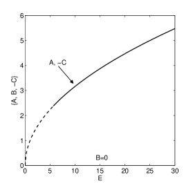
Figure 5: Amplitudes $A=-C$ and $B$ of the antisymmetric CW as functions of $E$.

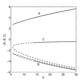
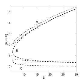
Figure 6: Amplitudes $A$, $B$ and $C$ as functions of $E$, for two families of asymmetric CW states. Due to the axes scale in panel (a), amplitude $A$ seems to be represented by a single (formally stable) curve, whereas it is actually composed of two close curves,originating from a common initial point at $E=5.66$, with a completely unstable lower branch, and the upper one being stable at $E>13.95$, $A>3.99$.

III.2 Symmetric lattice solitons

As said above, it is natural to expect that the nonlinear lattice supports, in addition to the exact CLSs (39), discrete solitons, which may be subject, in particular, to the symmetry constraint, $a_{n}=c_{n}$, satisfied at all $n$, or may be asymmetric. The discrete solitons are not compact modes, but they feature a strong exponential localization.

With the help of the numerical methods outlined above, several basic families of symmetric solitons have been detected. The first two families are illustrated by Fig. 7. While in one case (Fig. 7) both amplitudes $A_{n}$ and $C_{n}$ have a maximum with equal values at $n=-1$ and $n=0$, the other solution (Fig. 7) has a double maximum in terms of the $B$ amplitude. As concerns the stability, the family demonstrated in Fig. 7 was found to be stable, while the one shown in Fig. 7 is unstable. A systematic numerical analysis has shown that the family of the solitons with the double maximum in the $A_{n}=C_{n}$ fields bifurcates from the one characterized by the double maximum in $B_{n}$, through a typical supercritical bifurcation, see Fig. 8. Before the bifurcation occurs, i.e., at $E<2.90$, the solution is stable. Past the bifurcation, the upper branch, represented by the solitons shown in Fig. 7, destabilizes, while the lower one (see an example in Fig. 7) remains stable. An example for the evolution of unstable solitons from the upper branch is presented in Fig. 9. It is seen that the unstable soliton actually remains a localized mode, which features randomized intrinsic dynamics and emission of weak phonon waves. Figure 9 demonstrates that the strongly unstable solution is oscillating around a stable solution belonging to the lower branch, shown in Fig. 8. The oscillating unstable soliton emits spatially asymmetric radiation, due to asymmetric interference between the unstable and stable modes.

As $E$ decreases, the shape of the discrete solitons becomes Gaussian-like, i.e., quasi-continuous. This peculiarity can be seen in Fig. 7, for $E=2.90$, taken at the bifurcation point.

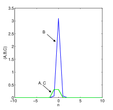
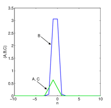
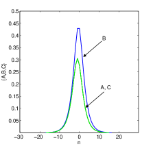
Figure 7: (Color online) Examples of the discrete symmetric solitons corresponding to the marked points in Fig. 8. Panels (a), (b) and (c) refer to points a ($E=10$, the stable lower branch), b ($E=10$, the unstable upper branch), and c ($E=2.90$, the bifurcation point), respectively. Amplitudes $A_{n}=C_{n}$ and $B_{n}$ are denoted, severally,by green and blue lines.

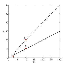
Figure 8: The stability of the first two families of symmetric discrete solitons, shown by means of the respective $N(E)$ curves. The marked points correspond to the solitons displayed in Fig. 7.

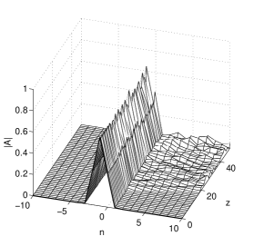
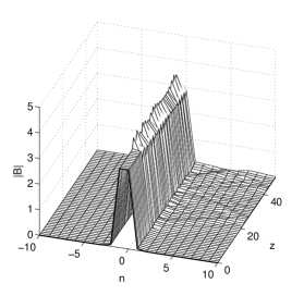
Figure 9: A typical example of the evolution of an unstable symmetric discrete soliton, belonging to the unstable upper branch in Fig. 8, with $E=10$. The stationary version of this soliton is shown in Fig. 7).

Two additional types of symmetric discrete solitons, found in the same model, are presented in Fig. 11. Both feature stability diagrams that consist of upper and lower branches merging into one, as shown in Fig. 10. The family exhibited in Figs. 10 and 11 is stable in the region of $E>15.46$, $N>69.87$ (the lower branch). An example of the evolution of an unstable soliton is shown in Fig. 12. It can be concluded that in this case too, the unstable discrete soliton remains an effectively localized mode with chaotic intrinsic dynamics, emitting small-amplitude phonon waves into the lattice. On the other hand, the second additional family, presented in Figs. 10, 11, is completely unstable.

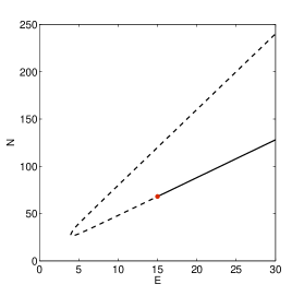
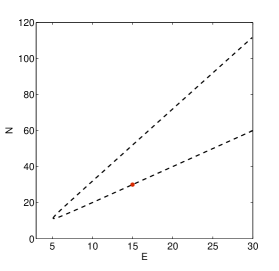
Figure 10: Two additional families of symmetric localized solitons, displayed by means of $N(E)$ curves.

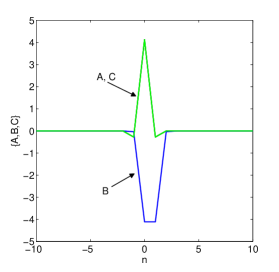
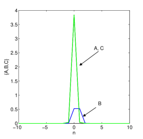
Figure 11: (Color online) Typical examples of profiles of the symmetric discrete solitons belonging to the additional families shown in Fig. 10. Panels (a) and (b) correspond to points marked on the lower branches in Figs. 10 and 10, respectively, both with $E=15$.

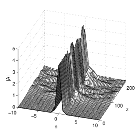
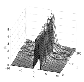
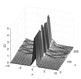
Figure 12: An example for the evolution of an unstable mode that belongs to the partially stable family in Fig. 10, with $E=15$ (Fig. 11 shows the unperturbed shape of this discrete soliton).

III.3 Extended compact antisymmetric states

Extended, but nevertheless compact, antisymmetric states, defined by condition $A_{n}=-C_{n}$, can be constructed as juxtapositions of the elementary CLS solution (39), with nonvanishing amplitudes in a finite set of lattice cells, where it has

$$A_{n}=\sqrt{E}=-C_{n},$$ (46)

and zero in all others, with all $B_{n}=0$. The total norm (3) of this extended state is given by an obvious expression,

$$N=2nE,$$ (47)

where $n$ denotes a number of cells with nonvanishing amplitudes $A_{n}$ and $C_{n}$. Examples for $n=1$ and $n=3$ are shown in Fig. 13. As mentioned in Section III.1, the antisymmetric CW solution may be considered as a limit case of this family, in the case when $n$ comprises the entire domain.

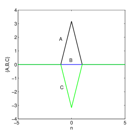
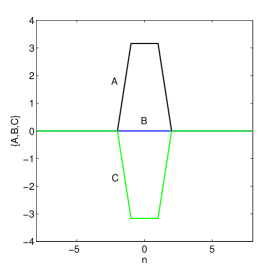
Figure 13: (Color online) Compact antisymmetric states extending to one cell (a) and three cells (b). Amplitudes $A$, $B$, and $C$ are denoted by black, blue and green lines, respectively.

These compact antisymmetric states are only partially stable. Systematic numerical analysis has shown that, for smaller values of propagation constant $E$ (and $N$), all solutions of this type are unstable. Specifically, for $n=1$ the solutions are stable at

$$E>6.18,N>12.36,$$ (48)

and for $n=3$ the stability region is

$$E>6.74,N>13.48.$$ (49)

In fact, Eqs. (48) and (49) define a nontrivial stability border for the compact modes in the nonlinear chain. A representative example of the dynamics of an unstable compact mode with $n=1$ and $E=5$ is displayed in Fig. 14, which shows that the instability destroys it.

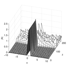
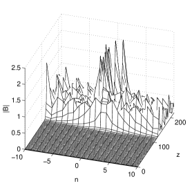
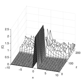
Figure 14: The evolution of an unstable compact antisymmetric discrete solution, whose stationary form is given by Eq. (46), with a single cell ($n=1$) and $E=5$.

III.4 Asymmetric lattice solitons

Numerous families of discrete asymmetric lattice states, with $\left|A_{n}\right|\neq\left|C_{n}\right|$, were discovered in the course of the numerical investigation. Two such fundamental families, which were found to be partially stable, are presented in Figs. 15-15 (the full stability diagrams) and in Fig. 16 (shape examples). Additionally, Figs. 15 and 15 present the asymmetry ratio, $\theta$, defined here as:

$$\theta=\frac{\sum_{-\infty}^{+\infty}\left(A_{n}^{2}-C_{n}^{2}\right)}{\sum_{-\infty}^{+\infty}\left(A_{n}^{2}+C_{n}^{2}\right)},$$ (50)

as a function of $E$, cf. the above definition for the single cell, given by Eq. (38).

In particular, the solutions displayed in Fig. 16, which may be referred to as asymmetric-symmetric modes, as they feature $\mathrm{sign}(A_{n})=\mathrm{sign}(C_{n})$, are stable in the region $E>4.14$, $N>4.7$ [the lower $N(E)\$branch]. The second family, which we name the asymmetric-antisymmetric solutions, with $\mathrm{sign}(A_{n})=-\mathrm{sign}(C_{n})$, shown in Fig. 16, is stable at $E>12.58$, $N>41.8$ (the lower branch).

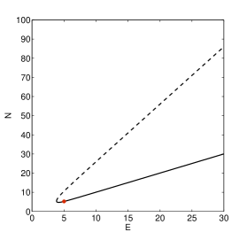
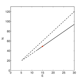
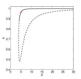
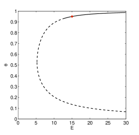
Figure 15: The total norm versus the propagation constant, $E$, for the families of asymmetric-symmetric lattice solitons (a) and asymmetric-antisymmetric ones (b) (see definitions in the text). The marked points correspond to the examples displayed in Fig. 16. (c,d): The same families as in (a,b), but shown by means of the $\theta(E)$ curves, where the asymmetry ratio, $\theta$, is defined in Eq. 50.

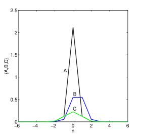
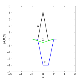
Figure 16: (Color online) Examples of profiles of (a) asymmetric-symmetric lattice solitons, and (b) asymmetric-antisymmetric ones. Panels (a) and (b) correspond to the marked points in the lower branches of the curves displayed in Figs. 15 ($E=5,N=5.2$) and 15 ($E=15,N=49.04$), respectively.

Other asymmetric lattice solitons were also found, two of which are presented in Fig. 17. While the family demonstrated in Fig. 17 is entirely unstable, the one displayed in Fig. 17 does have a stability region (not shown here explicitly).

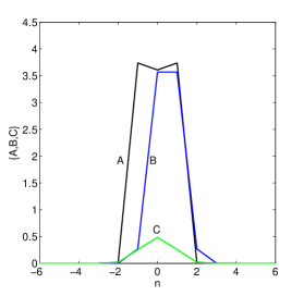
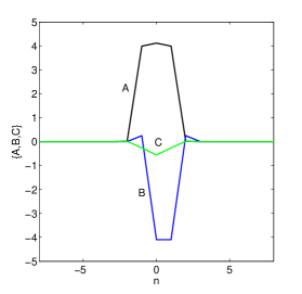
Figure 17: (Color online) Typical profiles of two asymmetric lattice solitons belonging to the two additional families, both with $E=15$.

Additional varieties of both symmetric and asymmetric localized states can be built by combining the lattice solitons found above (in particular, taking any of the four types of the asymmetric solitons mentioned here) and, accordingly, symmetric or asymmetric CW segments, taken from the CW states obtained in Section III.1, with an arbitrary number of lattice cells. An example of a so built extended confined asymmetric lattice mode is given in Fig. 18. This solution is a combination of the asymmetric-antisymmetric one, presented above in Figs. 15, 15, 16, and an eight-cell section of the asymmetric CW state, taken from Fig. 6. It can be checked that, for the stability of this combined solution, both its building blocks must be stable. In particular, for the combined mode shown here, the stability region is $E>13.88$, $N>300.10$, as its ingredients are stable in the same interval.

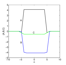
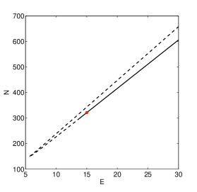
Figure 18: (color online) (a) An example an extended confined asymmetric state, for $E=15$. This mode is a combination of the localized asymmetric one from Fig. 16 and an 8-cells segment of the asymmetric CW from Fig. 6. (b) The stability diagram for the family of these extended confined asymmetric states. The marked point corresponds to the asymmetric state shown in panel (a).

IV The variational approximation for lattice solitons in the single infinite chain

IV.1 The formulation

A possibility to produce results for solitons in an analytical form, even if it is an approximate one, is obviously relevant. In this section we aim to develop a variational approximation (VA) for lattice solitons, and compare the so produced approximate analytical results to their numerical counterparts reported in the previous section. To this end, we note that the Lagrangian corresponding to Hamiltonian (14) is

$$L = \frac{i}{2}\sum_{n}\left(a_{n}^{\ast}\frac{da_{n}}{dz}-a_{n}\frac{da_{n}^{\ast}}{dz}\right)$$ (51)

$$+ \frac{i}{2}\sum_{n}\left(b_{n}^{\ast}\frac{db_{n}}{dz}-b_{n}\frac{db_{n}^{\ast}}{dz}\right)$$

$$+ \frac{i}{2}\sum_{n}\left(c_{n}^{\ast}\frac{dc_{n}}{dz}-c_{n}\frac{dc_{n}^{\ast}}{dz}\right)-H$$

$$\equiv -EN-H,$$

from which underlying equations (1) can be derived as standard Euler-Lagrange equations, with $E$ playing the role of the Lagrangian multiplier.

We apply the VA to stationary lattice solitons, following the general lines of Ref. MIW , where the VA was developed for solitons in the discrete nonlinear Schrödinger equation. The stability of stationary solutions can be tested by checking if they realize a local minimum of the Hamiltonian. The VA is based on the following two simplest ansätze applicable to discrete solitons, which differ by assuming the double maximum in components $b_{n}$ or $\left(a_{n},c_{n}\right)$:

$$\mathrm{I}:\left\{\begin{array}[]{c}a_{n}(z)=Ae^{-\eta\left|n-n_{0}\right|}e^{iEz},\\ b_{n}(z)=Be^{-\eta\left|n-n_{0}-\frac{1}{2}\right|}e^{iEz},\\ c_{n}(z)=Ce^{-\eta\left|n-n_{0}\right|}e^{iEz};\end{array}\right.$$ (52)

$$\mathrm{II}:\left\{\begin{array}[]{c}a_{n}(z)=Ae^{-\eta\left|n-n_{0}+\frac{1}{2}\right|}e^{iEz},\\ b_{n}(z)=Be^{-\eta\left|n-n_{0}\right|}e^{iEz},\\ c_{n}(z)=Ce^{-\eta\left|n-n_{0}+\frac{1}{2}\right|}e^{iEz},\end{array}\right.$$ (53)

where $n_{0}$ is an arbitrary integer coordinate of the soliton’s center. The ansätze contain four variational parameters: three amplitudes, $A$, $B$, $C$, and inverse width $\eta$.

As mentioned above, ansatz (52) can be used to describe stationary localized states with sharp ${A_{n},C_{n}}$ and flat-top $B_{n}$ profiles (see Figs. 7, 7 and 16), while ansatz (53) pertains to sharp $B_{n}$ and flat-top $\left\{{A}_{n}{,C}_{n}\right\}$ profiles, see Fig. 7). We substitute these ansätze into the Hamiltonian (14) and Lagrangian (51) and perform the summation analytically, which yields

$$H_{\mathrm{I}}=-\frac{2B\left(A+C\right)}{\sinh\left(\eta/2\right)}-\frac{B^{4}+\left(A^{4}+C^{4}\right)\cosh\left(2\eta\right)}{2\sinh\left(2\eta\right)},$$ (54)

$$L_{\mathrm{I}}=-\frac{E\left(B^{2}+\left(A^{2}+C^{2}\right)\cosh\left(\eta\right)\right)}{\sinh\left(\eta\right)}-H_{\mathrm{I}}~{};$$ (55)

$$H_{\mathrm{II}}=-\frac{2B\left(A+C\right)}{\sinh\left(\eta/2\right)}-\frac{A^{4}+C^{4}+B^{4}\cosh\left(2\eta\right)}{2\sinh\left(2\eta\right)},$$ (56)

$$L_{\mathrm{II}}=-\frac{E\left(A^{2}+C^{2}+B^{2}\cosh\left(\eta\right)\right)}{\sinh\left(\eta\right)}-H_{\mathrm{II}}.$$ (57)

The stationary states are predicted by numerically solving the corresponding Euler-Lagrange equations,

$$\frac{\partial L_{\mathrm{I,II}}}{\partial A}=\frac{\partial L_{\mathrm{I,II}}}{\partial B}=\frac{\partial L_{\mathrm{I,II}}}{\partial C}=\frac{\partial L_{\mathrm{I,II}}}{\partial\eta}=0.$$ (58)

IV.2 Comparison between variational and numerical results for the infinite chain

In Figs. 19 and 20 we compare the VA predictions and their numerical counterparts for stationary modes with sharp $\{A_{n},C_{n}\}$ and flat-top $B_{n}$ shapes, which are approximated by ansatz I [Eq. (52)] with norms $N=3$ and $N=8$, respectively. The VA predicts both symmetric and asymmetric solutions. One can conclude that the agreement is better for larger $N$. This conclusion is natural, as larger $N$ correspond to more self-compressed solitons, for which the simple exponential ansätze are more appropriate.

The second type of stationary solutions has flat $\{A_{n},C_{n}\}$ and sharp $B_{n}$ profiles, which can be approximated by ansatz II. In Figs. 21 and 22 we present the comparisons between the corresponding VA predictions and numerical results. We again conclude that a larger norm provides better agreement.

Results of the systematic comparison of the variational and numerical results are summarized in Figs. 23-24. In particular, the VA-predicted $N(E)$ curves are shown in Fig. 23 for families of symmetric and asymmetric lattice solitons. The solid and dashed curves again correspond to stable and unstable ones. Further, these curves are compared to their numerically found counterparts in Fig. 23. One can see that the VA predictions agree well with the numerical data taken from Figs. 8 and 15. As before, a larger propagation constant $E$ provides for better agreement.

Finally, in Fig. 24 we compare dependences $\theta(E)$ for the asymmetry parameter of the lattice solitons, defined as per Eq. (50). The respective numerical data are taken from Fig. 15.

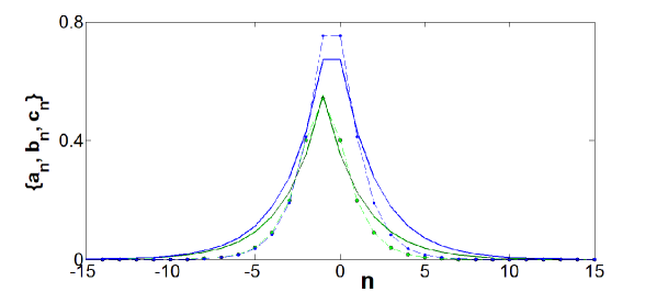
Figure 19: (Color online) Comparison between predictions of the VA based on ansatz (I) with $n_{0}=1$ (solid curves) and numerical results (dashed curves with small cicles). Here $N=3$, and the results are presented for symmetric lattice solitons. The respective values of the parameters are $E_{\mathrm{VA}}=3.014$, $E_{\mathrm{num}}=3.072$, and $H_{\mathrm{VA}}=8.665$, $H_{\mathrm{num}}=8.715$. The blue curves represent $B_{n}$, while the black and green ones correspond to $A_{n}$ and $C_{n}$, respectively.

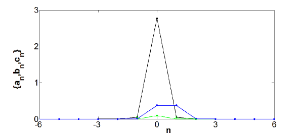
Figure 20: (Color online) The same as in Fig. 19, but for an asymmetric state with $N=8$ and $E_{\mathrm{VA}}=7.976$, $H_{\mathrm{VA}}=34.09$, $E_{\mathrm{num}}=7.966$, $H_{\mathrm{num}}=34.12$.

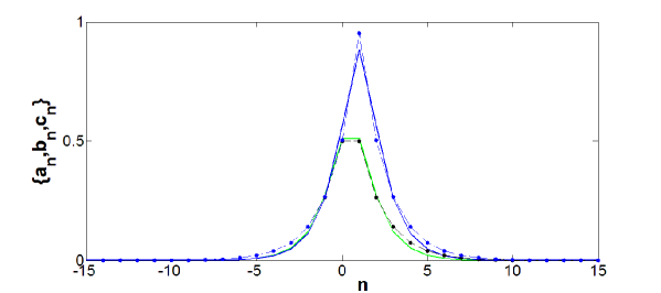
Figure 21: (Color online) The same as in Fig. 19, but for the variational predictions based on ansatz II with $n_{0}=-1$ and $N=3$, for symmetric lattice solitons. The parameters are $E_{\mathrm{VA}}=3.095$, $E_{\mathrm{num}}=3.107$, $H_{\mathrm{VA}}=8.703$, and $H_{\mathrm{num}}=8.726$.

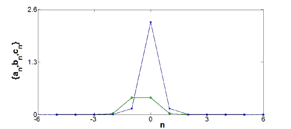
Figure 22: (Color online) The same as in Fig. 21, but with $n_{0}=0$, $N=6$ and $E_{\mathrm{VA}}=5.979$ and $H_{\mathrm{VA}}=22.059$, $E_{\mathrm{num}}=5.979$, $H_{\mathrm{num}}=22.059$.

Figure 23: (Color online) (a) The dependences $N(E)$ for lattice solitons, as predicted by the VA. The same dependences are compared to their numerically found counterparts in (b). Dashed pink curves in (a) and (b) represent unstable asymmetric solutions based on Ansatz I. Solutions of the same type but found numerically are represented by small pink stars in panel (b). Dotted black curves in (a) and (b) show unstable symmetric solutions based on Ansatz I. The corresponding numerical solutions are shown by black triangles in (b). Thin solid red curves in (a) and (b) indicate stable symmetric solutions produced by Ansatz II, while their numerical counterparts are shown by red squares in (b). Thick solid blue curves correspond to stable asymmetric solutions, produced by Ansatz I, whose numerical counterparts are displayed are bold blue dots in (b).

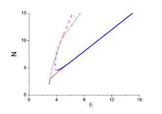
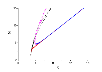
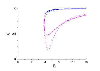
Figure 24: (Color online) The asymmetry parameters, $\theta(E)$, of lattice solitons. The solid blue curve is the branch of stable asymmetric solutions predicted by the VA, while the dashed pink curve corresponds to unstable ones. The corresponding numerical solutions are represented by dots and stars of the same colors.

V The linear double-chain model

A natural generalization of the model based on Eq. (1) is the double system, with each on-site amplitude $a_{n},b_{n},c_{n}$ replaced by the double set, $\left\{a_{n}^{(1)},a_{n}^{(2)}\right\},\left\{b_{n}^{(1)},b_{n}^{(2)}\right\},\left\{c_{n}^{(1)},c_{n}^{(2)}\right\}$, and linear mixing (Rabi coupling) applied at each site. Thus, Eqs. (11)-(12) are replaced by the double system,

$$i\frac{da_{n}^{(1,2)}}{dz}+\left(b_{n}^{(1,2)}+b_{n+1}^{(1,2)}\right)+\beta\left[|a_{n}^{(1,2)}|^{2}+\gamma|a_{n}^{(2,1)}|^{2}\right]a_{n}^{(1,2)}+\kappa_{ac}a_{n}^{(2,1)}=0,$$ (59)

$$i\frac{db_{n}^{(1,2)}}{dz}+\left(a_{n}^{(1,2)}+a_{n-1}^{(1,2)}+c_{n}^{(1,2)}+c_{n-1}^{(1,2)}\right)+\beta\left[|b_{n}^{(1,2)}|^{2}+\gamma|b_{n}^{(2,1)}|^{2}\right]b_{n}^{(1,2)}+\kappa_{b}b_{n}^{(2,1)}=0,$$ (60)

$$i\frac{dc_{n}^{(1,2)}}{dz}+\left(b_{n}^{(1,2)}+b_{n+1}^{(1,2)}\right)+\beta\left[|c_{n}^{(1,2)}|^{2}+\gamma|c_{n}^{(2,1)}|^{2}\right]c_{n}^{(1,2)}+\kappa_{ac}c_{n}^{(2,1)}=0,$$ (61)

where $\gamma\geq 0$ is the relative strength of the on-site XPM interaction.

In the BEC realization of the model, the on-site linear mixing between two hyperfine atomic states may be induced by a resonant GHz wave, hence in that case $\kappa_{ac}=\kappa_{b}\equiv\kappa$. In the BEC model, $\gamma=1$ is the most relevant value. In the optical realization, the two on-site modes may represent two different polarizations of light in the same waveguide. In the case of the linear polarizations, the linear mixing is imposed by the waveguide’s twist, the most relevant respective value of the XPM coefficient being $\gamma=2/3$; in the case of two circular polarizations, the mixing is imposed by an elliptic deformation of the waveguide’s cross section, $\gamma=2$ being the most relevant XPM value Agrawal . Alternatively, this system may correspond to the system of optical dual-core waveguides Christo , in which case $\gamma=0$. In the optics model, it is quite natural to have two different linear-mixing constants, $\kappa_{ac}\neq\kappa_{b}$.

For the double-chain model, the dispersion relation for modes $\sim\exp\left(iEz+ikx\right)$ takes the following form:

$$\begin{vmatrix}\ -E&\left(1+e^{ik}\right)&0&\kappa_{ac}&0&0\\ \left(1+e^{-ik}\right)&-E&\left(1+e^{-ik}\right)&0&\kappa_{b}&0\\ 0&\left(1+e^{ik}\right)&-E&0&0&\kappa_{ac}\\ \kappa_{ac}&0&0&-E&\left(1+e^{ik}\right)&0\\ 0&\kappa_{b}&0&\left(1+e^{-ik}\right)&-E&\left(1+e^{-ik}\right)\\ 0&0&\kappa_{ac}&0&\left(1+e^{ik}\right)&-E\end{vmatrix}=0$$ (62)

In the special case of $\kappa_{ac}=\kappa_{b}=\kappa$, Eq. (62) can be easily factorized:

$$\left(E^{2}-\kappa^{2}\right)\left[E^{4}-4\left(1+e^{ik}\right)\left(1+e^{-ik}\right)\left(E^{2}+\kappa^{2}\right)-2\kappa^{2}E^{2}+4\left(1+e^{ik}\right)^{2}\left(1+e^{-ik}\right)^{2}+\kappa^{4}\right]=0.$$ (63)

Then, two eigenvalues represent FBs, $E=\pm\kappa$, with the top and bottom signs corresponding to the symmetric and antisymmetric modes:

$$\left(a_{n}^{(1)},b_{n}^{(1)},c_{n}^{(1)}\right)=\pm\left(a_{n}^{(2)},b_{n}^{(2)},c_{n}^{(2)}\right),$$ (64)

while other eigenvalues produce dispersive branches, $E=\pm\kappa\pm 4\cos\left(k/2\right)$.

In the general case, with $\kappa_{ac}\neq\kappa_{b}$, the analysis of Eq. (62) is facilitated by considering symmetric and antisymmetric eigenstates, defined as per Eq. (64), which makes it possible to reduce the $6\times 6$ determinant in Eq. (62) to $3\times 3$ ones. In this general case, two eigenvalues corresponding to the split FBs are found in an exact form:

$$E=\pm\kappa_{ac},$$ (65)

and four dispersive branches are found exactly too:

$$E=\pm\frac{1}{2}\left(\kappa_{ac}+\kappa_{b}\right)\pm\frac{1}{2}\sqrt{\left(\kappa_{ac}-\kappa_{b}\right)^{2}+32\cos^{2}\left(k/2\right)}.$$ (66)

In both cases, the $\pm$ sign before the first term identifies the symmetric and antisymmetric eigenmodes, the $\pm$ sign in front of the second term being an independent one.

For the flatband states corresponding to eigenvalues (65), the eigenvectors can also be obtained in an exact form:

$$\psi_{n}^{\left(1\right)}=\pm\psi_{n}^{(2)}=\left(1,0,-1\right)f_{n},$$

where $f_{n}$ is an arbitrary discrete function. In such a case, the CLS, i.e., the single-cell excitation, corresponds to the following eigenvectors:

$$\psi_{n}^{\left(1\right)}=\frac{1}{\sqrt{2}}\left(1,0,-1\right)\delta_{n,n_{0}}=\pm\psi_{n}^{\left(2\right)},$$

cf. Eq. (9).

All the bands corresponding to Eqs. (65) and (66) are plotted in Fig. 25.

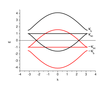
Figure 25: (Color online) Exactly found dispersion branches corresponding to the symmetric modes (black lines) and antisymmetric ones (red lines) in the double-diamond-chain system, plotted for (a) $\kappa_{ac}>\kappa_{b}$ ($\kappa_{ac}=1,\kappa_{b}=0.5$), and (b) $\kappa_{ac}<\kappa_{b}$ ($\kappa_{ac}=1,\kappa_{b}=1.5$). Flat-band states are represented by the horizontal lines, $E=\pm\kappa_{ac}$.

The linear system with broken symmetry between the top and bottom sites, $a$ and $c$, should also be mentioned. In that case, there are 3 different coupling constants $\kappa_{a}$, $\kappa_{b}$ and, $\kappa_{c}$ and the respective dispersion equation takes the form of

$$\begin{vmatrix}\ -E&\left(1+e^{ik}\right)&0&\kappa_{a}&0&0\\ \left(1+e^{-ik}\right)&-E&\left(1+e^{-ik}\right)&0&\kappa_{b}&0\\ 0&\left(1+e^{ik}\right)&-E&0&0&\kappa_{c}\\ \kappa_{a}&0&0&-E&\left(1+e^{ik}\right)&0\\ 0&\kappa_{b}&0&\left(1+e^{-ik}\right)&-E&\left(1+e^{-ik}\right)\\ 0&0&\kappa_{c}&0&\left(1+e^{ik}\right)&-E\end{vmatrix}=0,$$ (67)

cf. Eq. (62). The reduction based on Eq. (64) again allows one to reduce the $6\times 6$ determinant (67) to ones of size $3\times 3$, but the respective solutions turn out to be much more cumbersome than above. The respective eigenvalues have been analytically computed with the help of Mathematica, but are not included here. Effects of the on-site nonlinearity in the double-chain system, and the respective nonlinear modes, will be considered elsewhere.

VI Conclusion

The objective of this work is to report the development of the known FB (flatband) system, based on the “diamond chain”, in two directions: adding the on-site cubic nonlinearity, which is naturally present in the optical and matter-wave (BEC) implementation of the FB lattices, and, on the other hand, to introduce the double FB system, with two components coupled by the Rabi mixing at each lattice site. First, we have produced a full analytical solution for all stationary states (antisymmetric, symmetric, and asymmetric ones) in the system with three degrees of freedom, which represents an isolated nonlinear cell of the lattice. The asymmetric states emerge from their symmetric counterpart via a spontaneous-symmetry-breaking bifurcation, whose character is weakly subcritical. In the infinite nonlinear one-component chain, antisymmetric CLSs (compact localized states) of different lattice sizes, which are a hallmark of FB systems, have been found in an exact form too. Their stability was studied partly analytically (to demonstrate that they are not subject an antisymmetry-breaking bifurcation), and partly numerically, revealing a nontrivial stability boundaries for the compact modes, as given by Eqs. (48) and (49). These stability boundaries are specific to the nonlinear system. Along with the CLSs, various types of symmetric, antisymmetric and asymmetric CW (continuous-wave) states and lattice solitons (which are exponentially localized, but not compact modes) have been found too, in the numerical form and by dint of the VA (variational approximation). The VA for symmetric and asymmetric solitons demonstrates good accuracy, in comparison with their numerically generated shapes. It is found that different branches of the CW and soliton families may be completely or partly stable, some of them being fully unstable. Unstable lattice solitons typically evolve into confined quasi-soliton states, with randomized inner evolution, that emit small-amplitude phonon waves. Finally, an exact solution for eigenmodes of the linear double diamond chain was produced, with two split FBs present in the spectrum.

References

- (1) F. Lederer, G. I. Stegeman, D. N. Christodoulides, G. Assanto, M. Segev, and Y. Silberberg, Discrete solitons in optics, Phys. Rep. 463, 1 (2008).
- (2) S. Flach and A. V. Gorbach, Discrete breathers – advances in theory and applications, Phys. Rep. 467, 1 (2008).
- (3) Y. V. Kartashov, V. A. Vysloukh, and L. Torner, Soliton shape and mobility control in optical lattices, Progr. Opt. 52, 63 (2009).
- (4) P. G. Kevrekidis, The Discrete Nonlinear Schrödinger Equation: Mathematical Analysis, Numerical Computations, and Physical Perspectives (Springer: Berlin and Heidelberg, 2009).
- (5) F. Eilenberger, S. Minardi, A. Szameit, U. Röpke, J. Kobelke, K. Schuster, H. Bartelt, S. Nolte, A. Tünnermann, and T. Pertsch, Light bullets in waveguide arrays: spacetime-coupling, spectral symmetry breaking and superluminal decay, Opt. Exp. 19, 23171 (2011).
- (6) O. Derzhko, J. Richter and M. Maksymenko, Strongly correlated flat-band systems: The route from Heisenberg spins to Hubbard electrons, Int. J. Mod. Phys. B 29 1530007 (2015).
- (7) H. Tasaki, Ferromagnetism in the Hubbard models with degenerate single-electron ground states, Phys. Rev. Lett. 69, 1608 (1992); H. Tasaki, Stability of Ferromagnetism in the Hubbard Model, ibid. 73, 1158 (1994); K. Penc, H. Shiba, F. Mila, and T. Tsukagoshi, Ferromagnetism in multiband Hubbard models: From weak to strong Coulomb repulsion, Phys. Rev. B 54, 4056 (1996).
- (8) A. M. C. Souza and H. J. Herrmann, Flat-band localization in the Anderson-Falicov-Kimball model, Phys. Rev. B 79, 153104 (2009); C. Danieli, J. D. Bodyfelt and S. Flach, Flat-band engineering of mobility edges, ibid. 91, 235134 (2015).
- (9) K. Sun, Z. Gu, H. Katsura, and S. Das Sarma, Nearly Flatbands with Nontrivial Topology, Phys. Rev. Lett. 106, 236803 (2011); S. Yang, K. Sun, and S. Das Sarma, Quantum phases of disordered flatband lattice fractional quantum Hall systems, Phys. Rev. B 85, 205124 (2012).
- (10) H.-F. Zhang, S.-B. Liu, and X.-K. Kong, Study of the dispersive properties of three-dimensional photonic crystals with diamond lattices containing metamaterials, Laser Phys. 23, 105815 (2013).
- (11) D. Guzman-Silva, C. Mejia-Cortes, M. A. Bandres, M. C. Rechtsman, S. Weimann, S. Nolte, M. Segev, A. Szameit, and R. A. Vicencio, Experimental observation of bulk and edge transport in photonic Lieb lattices, New. J. Phys. 16, 063061 (2014).
- (12) N. Masumoto, N. Y. Kim, T. Byrnes, K. Kusudo, A. Löffer, S. Höfling, A. Forchel, and Y. Yamamoto, Exciton-polariton condensates with flat bands in a two-dimensional kagome lattice, New. J. Phys. 14, 065002 (2012).
- (13) T. Jacqmin, I. Carusotto, I. Sagnes, M. Abbarchi, D. D. Solnyshkov, G. Malpuech, E. Galopin, A. Lemaître, J. Bloch, and A. Amo, Direct Observation of Dirac Cones and a Flatband in a Honeycomb Lattice for Polaritons, Phys. Rev. Lett. 112, 116402 (2014); F. Baboux, L. Ge, T. Jacqmin, M. Biondi, E. Galopin, A. Lemaître, L. Le Gratiet, I. Sagnes, S. Schmidt, H. E. Türeci, A. Amo, and J. Bloch, Bosonic Condensation and Disorder-Induced Localization in a Flat Band, ibid. 116, 066402 (2016); A. Amo and J. Bloch, Exciton-polaritons in lattices: A non-linear photonic simulator, C. R. Physique 17, 934 (2016).
- (14) Y. Zhang and C. Zhang, Bose-Einstein condensates in spin-orbit-coupled optical lattices: Flat bands and superfluidity, Phys. Rev. A 87, 023611 (2013).
- (15) S. Taie, H. Ozawa, T. Ichinose, T. Nishio, S. Nakajima, and Y. Takahashi, Coherent driving and freezing of bosonic matter wave in an optical Lieb lattice, Sci. Adv. 1, e1500854 (2015).
- (16) D. Leykam, S. Flach, O. Bahat-Treidel, and A. S. Desyatnikov, Flat band states: Disorder and nonlinearity, Phys. Rev. B 88, 224203 (2013); S. Flach, D. Leykam, J. D. Bodyfelt, P. Matthies, and A. S. Desyatnikov, Detangling flat bands into Fano lattices, Europhys. Lett. 105, 30001 (2014); J. D. Bodyfelt, D. Leykam, C. Danieli, X. Yu and S. Flach, Flatbands under Correlated Perturbations, Phys. Rev. Lett. 113, 236403 (2014).
- (17) L. Morales-Inostroza and R. A. Vicencio, Simple method to construct flat-band lattices, Phys. Rev. A 94, 043831 (2016).
- (18) D. Leykam, J. D. Bodyfelt, A. S. Desyatnikov and S. Flach, Localization of weakly disordered flat band states, Eur. Phys. J. B 90, 1 (2017).
- (19) A. E. Miroshnichenko, S. Flach and Y. S. Kivshar, Fano resonances in nanoscale structures, Rev. Mod. Phys. 82, 2257 (2010).
- (20) R. A. Vicencio, C. Cantillano, L. Morales-Inostroza, B. Real, C. Mejía-Cortés, S. Weimann, A. Szameit, and M. I. Molina, Observation of Localized States in Lieb Photonic Lattices, Phys. Rev. Lett. 114, 245503 (2015).
- (21) S. Xia, Y. Hu, D. Song, Y. Zong, L. Tang, and Z. Chen, Demonstration of flat-band image transmission in optically induced Lieb photonic lattices, Opt. Lett. 41, 1435-1438 (2016).
- (22) Y. Zong, S. Xia, L. Tang, D. Song, Y. Hu, Y. Pei, J. Su, Y. Li, and Z. Chen, Observation of localized flat-band states in Kagome photonic lattices, Opt. Exp. 24, 8877-8885 (2016).
- (23) R. A. Vicencio and M. Johansson, Discrete flat-band solitons in the kagome lattice, Phys. Rev. A 87, 061803(R) (2013).
- (24) P. Beličev, G. Gligorić, A. Radosavljević, A. Maluckov, M. Stepić, R. A. Vicencio, and M. Johansson, Localized modes in nonlinear binary kagome ribbons, Phys. Rev. E 92, 052916 (2015).
- (25) S. Mukherjee, A. Spracklen, D. Choudhury, N. Goldman, P. Öhberg, E. Andersson, and R. R. Thomson, Observation of a Localized Flat-Band State in a Photonic Lieb Lattice, Phys. Rev. Lett. 114, 245504 (2015).
- (26) S. Weimann, L. Morales-Inostroza, B. Real, C. Cantillano, A. Szameit and R. A. Vicencio, Transport in Sawtooth photonic lattices, Opt. Lett. 41, 2414 (2016).
- (27) M. Johansson, U. Naether, and R. A. Vicencio, Compactification tuning for nonlinear localized modes in sawtooth lattices, Phys. Rev. E 92, 032912 (2015).
- (28) D. López-González and M. I. Molina, Linear and nonlinear compact modes in quasi-one-dimensional flatband systems, Phys. Rev. A 93, 043847 (2016).
- (29) G. Gligorić, A. Maluckov, Lj. Hadzievski, S. Flach, and B. A. Malomed, Nonlinear localized flat-band modes with spin-orbit coupling, Phys. Rev. B 94, 144302 (2016).
- (30) A. I. Maimistov, On Stability of flat band modes in a rhombic nonlinear optical waveguide array, J. Optics 19, 045502 (2017).
- (31) J. Hudock, P. G. Kevrekidis, B. A. Malomed, and D. N. Christodoulides, Discrete vector solitons in two-dimensional nonlinear waveguide arrays: Solutions, stability, and dynamics, Phys. Rev. E 67, 056618 (2003)
- (32) R. J. Ballagh, K. Burnett, and T. F. Scott, Theory of an Output Coupler for Bose-Einstein Condensed Atoms, Phys. Rev. Lett. 78, 1607 (1997); J. Williams, R. Walser, J. Cooper, E. Cornell, and M. Holland, Nonlinear Josephson-type oscillations of a driven, two-component Bose-Einstein condensate, Phys. Rev. A 59, R31(R) (1999); P. Öhberg and S. Stenholm, Internal Josephson effect in trapped double condensates ibid. 59, 3890 (1999); D. T. Son and M. A. Stephanov, Domain walls of relative phase in two-component Bose-Einstein condensates, ibid. 65, 063621 (2002); S. D. Jenkins and T. A. B. Kennedy, Dynamic stability of dressed condensate mixtures, ibid. 68, 053607 (2003); Q.-H. Park and J. H. Eberly, Nontopological vortex in a two-component Bose-Einstein condensate, ibid. 70, 021602(R) (2004).
- (33) G. Iooss, D. D. Joseph, Elementary Stability Bifurcation Theory (Springer: New York, 1980)
- (34) B. A. Malomed, editor, Spontaneous Symmetry Breaking, Self-Trapping, and Josephson Oscillations (Springer-Verlag: Berlin and Heidelberg, 2013).
- (35) B. A. Malomed and M. I. Weinstein, Soliton dynamics in the discrete nonlinear Schrödinger equation, Phys. Lett. A 220, 1 (1996); I. E. Papacharalampous, P. G. Kevrekidis, B. A. Malomed, and D. J. Frantzeskakis, Soliton collisions in the discrete nonlinear Schrödinger equation, Phys. Rev. E 68, 046604 (2003); D. J. Kaup, Variational solutions for the discrete nonlinear Schrödinger equation, Math. Comput. Simul. 69, 322 (2005).
- (36) G. P. Agrawal, Nonlinear Fiber Optics (Academic Press: San Diego, 1995).