An Empirical Analysis of Approximation Algorithms for the Euclidean Traveling Salesman Problem

Abstract

With applications to many disciplines, the traveling salesman problem (TSP) is a classical computer science optimization problem with applications to industrial engineering, theoretical computer science, bioinformatics, and several other disciplines [2]. In recent years, there have been a plethora of novel approaches for approximate solutions ranging from simplistic greedy to cooperative distributed algorithms derived from artificial intelligence. In this paper, we perform an evaluation and analysis of cornerstone algorithms for the Euclidean TSP. We evaluate greedy, 2-opt, and genetic algorithms. We use several datasets as input for the algorithms including a small dataset, a medium-sized dataset representing cities in the United States, and a synthetic dataset consisting of 200 cities to test algorithm scalability. We discover that the greedy and 2-opt algorithms efficiently calculate solutions for smaller datasets. Genetic algorithm has the best performance for optimality for medium to large datasets, but generally have longer runtime. Our implementations is public available .

1 Introduction

Known to be NP-hard, the traveling salesman problem (TSP) was first formulated in 1930 and is one of the most studied optimization problems to date [8]. The problem is as follows: given a list of cities and a distance between each pair of cities, find the shortest possible path that visits every city exactly once and returns to the starting city. The TSP has broad applications including: shortest-path for lasers to sculpt microprocessors and delivery logistics for mail services, to name a few.

The TSP is an area of active research. In fact, several variants have been derived from the original TSP. In this paper, we focus on the Euclidean TSP. In the Euclidean TSP, the vertices correspond to points in a $d$-dimensional space, and the cost function is the Euclidean distance. That is, the Euclidean distance between two cities $x=(x_{1},x_{2},...,x_{d}),y=(y_{1},y_{2},...,y_{d})$ is:

$$(\sum_{i=0}^{d}(x_{i}-y_{i})^{2})^{1/2}$$ (1)

This simplification allows us to survey several cornerstone algorithms without introducing complex scenarios. The remainder of this paper is organized as follows. In Section 2, we briefly review the first solutions and survey variants to the TSP. We describe the algorithms used in our experiment in Section 3. A description of the benchmark datasets and results of the experiment are detailed in Section 4, and explains the findings and compares the performance of the algorithms. We then conclude and describe future work in Section 5.

2 Background

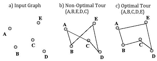
An example TSP is illustrated in Figure 1. The input is a collection of cities in the two dimensional space. This input can be represented as a distance matrix for each pair of cities or as a list of points denoting the coordinate of each city. In the latter method, distances are calculated using Euclidean geometry. A non-optimal tour is shown in sub-figure (b). Although not shown in the figure, each edge will have some non-negative edge weight denoting the distance between two nodes or cities. Due to the computational complexity of the TSP, it may be necessary to approximate the optimal solution. The optimal tour is shown in sub-figure (c). For small graphs, it may be possible to perform an exhaustive search to obtain the optimal solution. However, as the number of cities increases, so does the solutions space, problem complexity, and running time.

Figure 1:

If $n$ is the number of cities. The number of possible edges is $\sum_{i=0}^{n-1}i$. The number of possible tours is $(n-1)!/2$. since the same tour, with start point X and Y appears twice: once with X as the start node and once with Y as the start node.

The TSP was first formulated in the 1930s by Karl Menger in Vienna and Harvard. By the mid-1950s, solutions for TSP began to appear. The first solution was published by Dantzig, Fulkerson, and Johnson using a dataset of 49 cities. In 1972, Richard M. Karp proved that the Hamiltonian cycle problem was NP-Complete, which proves that the TSP is NP-Hard.

In modern day, the TSP has a variety of applications to numerous fields. Examples among these applications include genome sequencing, air traffic control, supplying manufacturing lines, and optimization.

3 Algorithms

We now move to a discussion of the algorithms used in our evaluation. First, we describe an upper bound for TSP in Section 3.1. The traditional greedy and 2-opt approaches are discussed in Section 3.2 and Section 3.3. We finally discuss the genetic algorithm in Section 3.4.

3.1 Random Path

Finding the worst case of TSP is as hard as the best one. So we uniformly generate a random path for all available edges, and use this as a upper bound of optimal path benchmark for all other algorithms.

3.2 Greedy Algorithm

The greedy heuristic is based on Kruskal’s algorithm to give an approximate solution to the TSP [11]. The algorithm forms a tour of the shortest route and can be constructed if and only if: The edges of the tour must not form a cycle unless the selected number of edges is equal to the number of vertices in the graph. The selected edge (before being appended to the tour) does not increase the degree of any node to be more than 2. The algorithm begins by sorting all edges from least weight to most heavily weighted. After the edges are sorted, the least heavily-weighted edge is selected and it is added to the tour if it does not violate the above conditions. The algorithm continues by selecting the next least-cost edge and adding it to the tour. This process is repeated until all vertices can be reached by the tour. The result is a minimum spanning tree and is a solution for the TSP. The runtime for the greedy algorithm is $O(n^{2}log(n))$ and generally returns a solution within 15-20% of the Held-Karp lower bound [15].

3.3 2opt Algorithm

In optimization, 2-opt is a simple local search algorithm first proposed by Croes in 1958 for solving the TSP [5]. The main idea behind it is to take a route that crosses over itself and reorder it so that it does not.

A complete 2-opt local search will compare every possible valid combination of the swapping mechanism. This technique can be applied to the travelling salesman problem as well as many related problems. These include the vehicle routing problem (VRP) as well as the capacitated VRP, which require minor modification of the algorithm.

This is the mechanism by which the 2-opt swap manipulates a given route:

1. take route[1] to route[i-1] and add them in order to new route

2. take route[i] to route[k] and add them in reverse order to new route

3. take route[k+1] to end and add them in order to new route

4. return new route

3.4 Genetic Algorithm

Genetic algorithms (GA) are search heuristics that at- tempt to mimic natural selection for many problems in optimization and artificial intelligence [6]. In a genetic algorithm, a population of candidate solutions is evolved over time towards better solutions. These evolutions generally occur through mutations, randomization, and recombination. We define a fitness function to differentiate between better and worse solutions. Solutions, or individuals, with higher fitness scores are more likely to survive over time. The final solution is found if the population converges to a solution within some threshold. However, great care must be taken to avoid being trapped at local optima.

We will now apply a genetic algorithm to the TSP [3]. We define a fitness function F as the length of the tour. Supposed we have an ordering of the cities $A={x_{1},x_{2},...,x_{n}}$ where n is the number of cities. The fitness score for the TSP becomes the cost of the tour $d(x,y)$ denote the distance from x to y.

$$F(A)=\sum_{i=0}^{n-1}d(x_{i},x_{i+1})+d(x_{n},x_{0})$$ (2)

The genetic algorithm begins with an initial, $P_{0}$ , random population of candidate solutions. That is, we have a set of paths that may or may not be good solutions. We then move forward one time step. During this time step, we perform a set of probabilistic and statistical methods to select, mutate, and produce an offspring population, $P_{1}$ , with traits similar to those of the best individuals (with the highest fitness) from $P_{0}$ . We then repeat this process until our population becomes homogeneous.

The running time of genetic algorithms is variable and dependent on the problem and heuristics used. However, for each individual in the population, we require $O(n)$ space for storage of the path. For genetic crossover, the space requirement remains $O(n)$. The best genetic algorithms can find solutions within 2% of the optimal tour for certain graphs [9].

4 Experiment

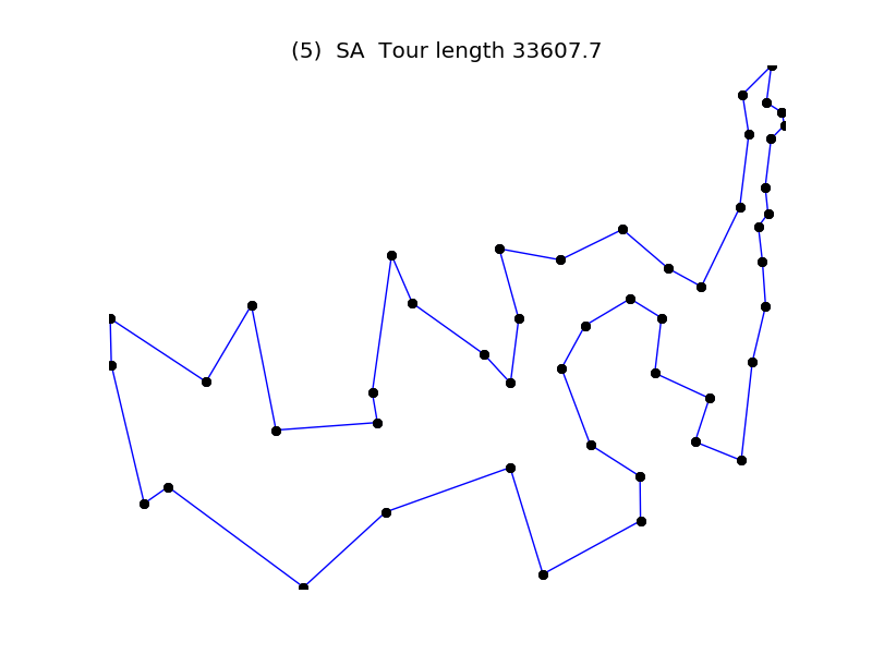
We benchmark our algorithms using publicly available datasets. Additionally, to test the scalability of the algorithms, we generated a synthetic dataset consisting of 200 cities. In all dataset names, the numeric digits represent the number of cities in the dataset. The datasets are as follows: P15, ATT48, and R200. All datasets except R200 can be found online [4, 14]. The ATT48 and SGB128 datasets represent real-data consisting of locations of cities in the United States. A visual representation of the ATT48 dataset in the 2D plane is shown in Figure 2

Figure 2: the ATT48 dataset in the 2D plane. (the United States)

Not all datasets have a known optimal tour. When this is the case, we use random path algorithm to infer a upper bound of the optimal tour.

4.1 Random Dataset

The R200 dataset was generated by plotting 200 random, uniformly distributed points $(x,y)$, in $R^{2}$ with $(x,y)\in[0,4000]$. As a result, all distances satisfy the triangle inequality and this dataset can be classified as a Euclidean TSP dataset. The running time for creating the dataset is $O(n)$. The output is a list of all cities represented as $(x,y)$ points.

4.2 Comparison

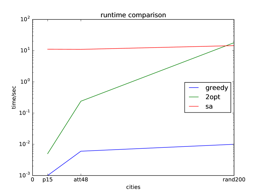
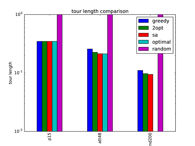
As we can see in Figure 3, the greedy is the most efficient. In Figure 4, we can see that most algorithms return a solution similar with the optimal for small datasets and become worse for larger datasets.

Figure 3: runtime comparison, the y axis is in log scale

In terms of running time (Figure 3), the best algorithm is greedy algorithm. However, in terms of optimal tour length of solution, the best algorithm is GA. This is in line with our expectations and alludes to the fact that different heuristics are better suited for different situations.

Figure 4: tour length comparison, the y axis is in log scale, divided by random tour length

As shown in Figure 4, genetic algorithm performs fairly consistently, in comparison to the 2-opt and greedy algorithms, across all datasets. Highlighted in Figure 3, the running time of genetic is almost linear. This suggests that for larger datasets, if running time is a concern, then the genetic algorithm should be used. Figure 4 further demonstrates that genetic algorithm maintains a smaller percent above optimal than the other algorithms. From this, we can see that genetic algorithm has high accuracy and better complexity than other heuristics, especially for larger datasets. Surprisingly, genetic algorithm got the optimal solution for att48 dataset, shown in Figure 5.

Figure 5: Solution generated by genetic algorithm for att48 dataset

5 Conclusion

Most of our algorithms attempt to solve the TSP in a linear fashion. Originating from artificial intelligence, the genetic algorithm is very different compared to greedy, and 2-opt. Literature suggests that the best algorithms focus on iteration and convergence to find optimal tours – something genetic algorithms attempt to achieve. For example, the Large Step Markov Chain [10] relies on Markov chains to find convergence of many paths to form a global optimum and several papers cite Markov Chains as the best known solution to TSP. Recent studies include using adaptive Markov Chain Monte Carlo algorithms [13]. Many of these extend the Metropolis algorithm [9], a simulated annealing algorithm which attempts to mimic randomness with particles as the temperature varies. This further supports our conclusion that algorithms inspired from artificial intelligence perform well for finding solutions for the TSP. However, these may not be suitable when a guarantee is required.

In this paper, we surveyed several key cornerstone approaches to the TSP. We selected four well-known algorithms and tested their performance on a variety of public datasets. Our results suggest that genetic algorithms (and other approaches from artificial intelligence) are able to find a near-optimal solution.

References

- [1] S. Arora. Polynomial time approximation schemes for euclidean tsp and other geometric problems. In Foundations of Computer Science, 1996. Proceedings., 37th Annual Symposium on, pages 2–11. IEEE, 1996.
- [2] BaoJunpeng. Introduction to Artificial Intelligence. [M].BeiJing:MachineryIn-dustryPress, 2010.
- [3] K. Bryant and A. Benjamin. Genetic algorithms and the traveling salesman problem. Department of Mathematics, Harvey Mudd College, pages 10–12, 2000.
- [4] J. Burkardt. Data for the traveling salesperson problem, 2011. http://people.sc.fsu.edu/ jburkardt/datasets/tsp/tsp.html.
- [5] G. A. Croes. A method for solving traveling-salesman problems. Operations research, 6(6):791–812, 1958.
- [6] J. Grefenstette, R. Gopal, B. Rosmaita, and D. Van Gucht. Genetic algorithms for the traveling salesman problem. In Proceedings of the first International Conference on Genetic Algorithms and their Applications, pages 160–168. Lawrence Erlbaum, New Jersey (160-168), 1985.
- [7] A. Haque, J. Shah, F. Ejaz, and J. X. Xu. An empirical evaluation of approximation algorithms for the metric traveling salesman problem.
- [8] A. Hoffman, J. Wolfe, R. Garfinkel, D. Johnson, C. Papadimitriou, P. Gilmore, E. Lawler, D. Shmoys, R. Karp, J. Steele, et al. The traveling salesman problem: a guided tour of combinatorial optimization. J. Wiley & Sons, 1986.
- [9] A. Homaifar, S. Guan, and G. E. Liepins. Schema analysis of the traveling salesman problem using genetic algorithms. Complex Systems, 6(6):533–552, 1992.
- [10] I. Hong, A. B. Kahng, and B.-R. Moon. Improved large-step markov chain variants for the symmetric tsp. Journal of Heuristics, 3(1):63–81, 1997.
- [11] B.-I. Kim, J.-I. Shim, and M. Zhang. Comparison of tsp algorithms. Project for Models in Facilities Planning and Materials Handling, 1998.
- [12] M. Mucha. frac 139-approximation for graphic tsp. Theory of computing systems, 55(4):640–657, 2014.
- [13] F. Qiu, J. Zhang, and H. Yan. An adaptive markov chain monte carlo algorithm for tsp. In Computer Science and Software Engineering, 2008 International Conference on, volume 1, pages 439–442. IEEE, 2008.
- [14] G. Reinelt. Tsplib, 1995. http://comopt.ifi.uni-heidelberg.de/software/TSPLIB95/.
- [15] D. J. Rosenkrantz, R. E. Stearns, and P. M. Lewis, II. An analysis of several heuristics for the traveling salesman problem. SIAM journal on computing, 6(3):563–581, 1977.