Expectation Propagation for t-Exponential Family Using Q-Algebra

Abstract

Exponential family distributions are highly useful in machine learning since their calculation can be performed efficiently through natural parameters. The exponential family has recently been extended to the t-exponential family, which contains Student-t distributions as family members and thus allows us to handle noisy data well. However, since the t-exponential family is defined by the deformed exponential, we cannot derive an efficient learning algorithm for the t-exponential family such as expectation propagation (EP). In this paper, we borrow the mathematical tools of q-algebra from statistical physics and show that the pseudo additivity of distributions allows us to perform calculation of t-exponential family distributions through natural parameters. We then develop an expectation propagation (EP) algorithm for the t-exponential family, which provides a deterministic approximation to the posterior or predictive distribution with simple moment matching. We finally apply the proposed EP algorithm to the Bayes point machine and Student-t process classification, and demonstrate their performance numerically.

1 Introduction

Exponential family distributions play an important role in machine learning, due to the fact that their calculation can be performed efficiently and analytically through natural parameters or expected sufficient statistics [1]. This property is particularly useful in the Bayesian framework since a conjugate prior always exists for an exponential family likelihood and the prior and posterior are often in the same exponential family. Moreover, parameters of the posterior distribution can be evaluated only through natural parameters.

As exponential family members, Gaussian distributions are most commonly used because their moments, conditional distribution, and joint distribution can be computed analytically. Gaussian processes are a typical Bayesian method based on Gaussian distributions, which are used for various purposes such as regression, classification, and optimization [2]. However, Gaussian distributions are sensitive to outliers. It is also known that heavier-tailed distributions are often more preferred in practice and Student-t distributions would be good alternatives to Gaussian distributions [3]. Similarly Student-t processes would also be promising alternatives to Gaussian processes [4].

The problem of the Student-t distribution is that it does not belong to the exponential family unlike the Gaussian distribution and thus cannot enjoy good properties of the exponential family. For this problem, the exponential family was recently generalized to the t-exponential family [5], which contains Student-t distributions as family members. Following this line, the Kullback-Leibler divergence was generalized to the t-divergence, and approximation methods based on t-divergence minimization have been explored [6]. However, the t-exponential family does not allow us to employ standard useful mathematical tricks, e.g., logarithmic transformation does not reduce the product of t-exponential family functions into summation. For this reason, the t-exponential family unfortunately does not inherit an important property of the original exponential family, that is, calculation can be performed through natural parameters. Furthermore, while the dimensionality of sufficient statistics is the same as that of the natural parameters in the exponential family and thus there is no need to increase the parameter size to incorporate new information [7], this useful property does not hold in the t-exponential family.

The purpose of this paper is to further explore mathematical properties of natural parameters of the t-exponential family through pseudo additivity of distributions based on q-algebra used in statistical physics [8][9]. More specifically, our contributions in this paper are three-fold:

1. We show that, in the same way as ordinary exponential family distributions, q-algebra allows us to handle the calculation of t-exponential family distributions through natural parameters.

2. Our q-algebra based method enables us to extend assumed density filtering (ADF) [6] and develop an algorithm of expectation propagation (EP) [10] for the t-exponential family. In the same way as the original EP algorithm for ordinary exponential family distributions, our EP algorithm provides a deterministic approximation to the posterior or predictive distribution for t-exponential family distributions with simple moment matching.

3. We apply the proposed EP algorithm to the Bayes point machine [10] and Student-t process classification, and we demonstrate their usefulness as alternatives to the Gaussian approaches numerically.

2 t-exponential Family

In this section, we review the t-exponential family [5][6], which is a generalization of the exponential family.

The t-exponential family is defined as follows,

$$p(x;\theta) = \exp_{t}(\langle\Phi(x),\theta\rangle-g_{t}(\theta)),$$ (1)

where $\exp_{t}(x)$ the deformed exponential function defined as

$$\exp_{t}(x) = \left\{\begin{array}[]{ll}\exp(x)&\mathrm{if~{}}t=1,\\ [1+(1-t)x]^{\frac{1}{1-t}}&\mathrm{otherwise},\end{array}\right.$$ (4)

and $g_{t}(\theta)$ is the log-partition function that satisfies

$$\nabla_{\theta}g_{t}(\theta)=\mathbb{E}_{q}[\Phi(x)].$$ (5)

The notation $\mathbb{E}_{q}$ denotes the expectation over $q(x)$, where $q(x)$ is the escort distribution of $p(x)$ defined as

$$q(x)=\frac{p(x)^{t}}{\int p(x)^{t}\mathrm{d}x}.$$ (6)

We call $\theta$ a natural parameter and $\Phi(x)$ a sufficient statistics.

Let us express the $k$-dimensional Student-t distribution with $v$ degrees of freedom as

$$\mathrm{St}(x;v,\mu,\Sigma)=\frac{\Gamma((v+k)/2)}{(\pi v)^{k/2}\Gamma(v/2)|\Sigma|^{1/2}}\biggl{(}1+(x-\mu)^{\top}|v\Sigma|^{-1}(x-\mu)\biggr{)}^{-\frac{v+k}{2}},$$ (7)

where $\Gamma(x)$ is the gamma function, $|A|$ is the determinant of matrix $A$, and $A^{\top}$ is the transpose of matrix $A$. We can confirm that the Student-t distribution is a member of the t-exponential family as follows. First, we have

$$\mathrm{St}(x;v,\mu,\Sigma)=\bigl{(}\Psi+\Psi\cdot(x-\mu)^{\top}(v\Sigma)^{-1}(x-\mu)\bigr{)}^{\frac{1}{1-t}},$$ (8)

$${\rm where\ \ }\Psi=\Biggl{(}\frac{\Gamma((v+k)/2)}{(\pi v)^{k/2}\Gamma(v/2)|\Sigma|^{1/2}}\Biggr{)}^{1-t}.$$ (9)

Note that relation $-(v+k)/2=1/(1-t)$ holds, from which we have

$$\langle\Phi(x),\theta\rangle = \Biggl{(}\frac{\Psi}{1-t}\Biggr{)}(x^{\top}Kx-2\mu^{\top}Kx),$$ (10)

$$g_{t}(\theta) = -\Biggl{(}\frac{\Psi}{1-t}\Biggr{)}(\mu^{\top}K\mu+1)+\frac{1}{1-t},$$ (11)

where $K=(v\Sigma)^{-1}$. Second, we can express the Student-t distribution as a member of the t-exponential family:

$$\mathrm{St}(x;v,\mu,\Sigma)=\bigl{(}1+(1-t)\langle\Phi(x),\theta\rangle-g_{t}(\theta)\bigr{)}^{\frac{1}{1-t}}=\exp_{t}\bigl{(}\langle\Phi(x),\theta\rangle-g_{t}(\theta)\bigr{)}.$$ (12)

If $t=1$, the deformed exponential function is reduced to the ordinary exponential, and therefore the t-exponential family is reduced to the ordinary exponential family, which corresponds to the Student-t distribution with infinite degrees of freedom. For t-exponential family distributions, a divergence is defined as follows [6]:

$$D_{t}(p\|\tilde{p})=\int q(x)\ln_{t}p(x)-q(x)\ln_{t}\tilde{p}(x)\mathrm{d}x,$$ (13)

where $\ln_{t}x:=\frac{x^{1-t}-1}{1-t}\ \ (x\geq 0,t\in\mathbb{R}^{+})$. This is called the t-divergence and $q(x)$ is the escort function of $p(x)$.

3 Assumed Density Filtering and Expectation Propagation

We briefly review the assumed density filtering (ADF) and expectation propagation (EP) [10].

Let $D=\{(x_{1},y_{1}),\ldots,(x_{i},y_{i})\}$ be input-output paired data. We denote the likelihood for the $i$-th data as $l_{i}(w)$ and the prior distribution of parameter $w$ as $p^{(0)}(w)$. The total likelihood is given as $\prod_{i}l_{i}(w)$ and the posterior distribution can be expressed as $p(w|D)\propto p^{(0)}(w)\prod_{i}l_{i}(w)$.

3.1 Assumed Density Filtering

ADF is an online approximation method for the posterior distribution.

Suppose that $i-1$ samples $(x_{1},y_{1}),\ldots,(x_{i-1},y_{i-1})$ have already been processed and an approximation to the posterior distribution, $\tilde{p}_{i-1}(w)$, has already been obtained. Given the $i$-th sample $(x_{i},y_{i})$, the posterior distribution $p_{i}(w)$ can be obtained as

$$p_{i}(w)\propto\tilde{p}_{i-1}(w)l_{i}(w).$$ (14)

Since the true posterior distribution $p_{i}(w)$ cannot be obtained analytically, it is approximated in ADF by minimizing the Kullback-Leibler (KL) divergence from $p_{i}(w)$ to its approximation:

$$\tilde{p}_{i}=\mathop{\mathrm{arg~{}min}}\limits_{\tilde{p}}\mathrm{KL}(p_{i}\|\tilde{p}).$$ (15)

Note that if $\tilde{p}$ is an exponential family members, the above calculation is reduced to moment matching.

3.2 Expectation Propagation

Although ADF is an effective method for online learning, it is not favorable for non-online situations, because the approximation quality depends heavily on the permutation of data. To overcome this problem, EP was proposed.

In EP, an approximation of the posterior that contains whole data terms is prepared beforehand, typically as a product of data-corresponding terms:

$$\tilde{p}(w)=\frac{1}{Z}p^{(0)}(w)\prod_{i}\tilde{l}_{i}(w),$$ (16)

where $Z$ is the normalizing constant. In the above expression, factor $\tilde{l}_{i}(w)$, which is often called a site approximation, corresponds to the local likelihood $l_{i}(w)$. If $\tilde{l}_{i}(w)$ is an exponential family member, the total approximation also belongs to the exponential family.

Differently from ADF, in EP, these site approximations are updated iteratively in four steps as follows. First, when we update site $\tilde{l}_{j}(w)$, we eliminate the effect of site $j$ from the total approximation as

$$\tilde{p}^{\backslash j}(w)\propto\frac{\tilde{p}(w)}{\tilde{l}_{j}(w)},$$ (17)

where $\tilde{p}^{\backslash j}(w)$ is often called a cavity distribution. If an exponential family distribution is used, the above calculation is reduced to the subtraction of natural parameters. Second, we incorporate likelihood $l_{j}(w)$ by minimizing the divergence $\mathrm{KL}$$(\tilde{p}^{\backslash j}(w)$$l_{j}(w)/Z^{\setminus j}$$\|\tilde{p}(w))$, where $Z^{\setminus j}$ is the normalizing constant. Note that this minimization is reduced to moment matching for the exponential family. After this step, we obtain $\tilde{p}(w)$. Third, we exclude the effect of terms other than $j$, which is equivalent to calculating a cavity distribution as $\tilde{l}_{j}(w)^{\mathrm{new}}\propto\frac{\tilde{p}(w)}{\tilde{p}^{\setminus j}(w)}$ Finally, we update the site approximation by replacing $\tilde{l}_{j}(w)$ by $\tilde{l}_{j}(w)^{\mathrm{new}}$.

Note again that calculation of EP is reduced to addition or subtraction of natural parameters for the exponential family.

3.3 ADF for t-exponential Family

ADF for the t-exponential family was proposed in [6], which uses the t-divergence instead of the KL divergence:

$$\tilde{p}=\mathop{\mathrm{arg~{}min}}\limits_{p^{\prime}}D_{t}(p\|p^{\prime})=\int q(x)\ln_{t}p(x)-q(x)\ln_{t}p^{\prime}(x;\theta)\mathrm{d}x.$$ (18)

When an approximate distribution is chosen from the t-exponential family, we can utilize the property $\nabla_{\theta}g_{t}(\theta)=\mathbb{E}_{\tilde{q}}(\Phi(x))$, where $\tilde{q}$ is the escort function of $q(x)$. Then, minimization of the t-divergence yields

$$\mathbb{E}_{q}[\Phi(x)]=\mathbb{E}_{\tilde{q}}[\Phi(x)].$$ (19)

This is moment matching, which is a celebrated property of the exponential family. Since the expectation is respect to the escort function, this is called escort moment matching.

As an example, let us consider the situation where the prior is the Student-t distribution and the posterior is approximated by the Student-t distribution: $p(w|D)\cong\tilde{p}(w)=\mathrm{St}(w;\tilde{\mu},\tilde{\Sigma},v)$. The approximated posterior $\tilde{p}_{i}(w)=\mathrm{St}(w;\tilde{\mu}^{(i)},\tilde{\Sigma}^{i},v)$ can be obtained by minimizing the t-divergence from $p_{i}(w)\propto\tilde{p}_{i-1}(w)\tilde{l}_{i}(w)$ as

$$\mathop{\mathrm{arg~{}min}}\limits_{\mu^{\prime},\Sigma^{\prime}}D_{t}(p_{i}(w)\|\mathrm{St}(w;\mu^{\prime},\Sigma^{\prime},v)).$$ (20)

This allows us to obtain an analytical update expression for t-exponential family distributions.

4 Expectation Propagation for t-exponential Family

As shown in the previous section, ADF has been extended to EP (which resulted in moment matching for the exponential family) and to the t-exponential family (which yielded escort moment matching for the t-exponential family). In this section, we combine these two extensions and propose EP for the t-exponential family.

4.1 Pseudo Additivity and Q-Algebra

Differently from ordinary exponential functions, deformed exponential functions do not satisfy the product rule:

$$\exp_{t}(x)\exp_{t}(y)\neq\exp_{t}(x+y).$$ (21)

For this reason, the cavity distribution cannot be computed analytically for the t-exponential family.

On the other hand, the following equality holds for the deformed exponential functions:

$$\exp_{t}(x)\exp_{t}(y)=\exp_{t}(x+y+(1-t)xy),$$ (22)

which is called pseudo additivity.

In statistical physics [8][9], a special algebra called q-algebra has been developed to handle a system with pseudo additivity. We will use the q-algebra for efficiently handling t-exponential distributions.

Definition 1 (q-product)

Operation $\otimes_{q}$ called the q-product is defined as

$$x\otimes_{q}y:=\left\{\begin{array}[]{ll}[x^{1-q}+y^{1-q}-1]^{\frac{1}{1-q}}&\mathrm{if~{}}x>0,y>0,x^{1-q}+y^{1-q}-1>0,\\ 0&\mathrm{otherwise}.\end{array}\right.$$ (23)

Definition 2 (q-division)

Operation $\oslash_{q}$ called the q-division is defined as

$$x\oslash_{q}y:=\left\{\begin{array}[]{ll}[x^{1-q}-y^{1-q}-1]^{\frac{1}{1-q}}&\mathrm{if~{}}\ x>0,y>0,x^{1-q}-y^{1-q}-1>0,\\ 0&\mathrm{otherwise}.\end{array}\right.$$ (24)

Definition 3 (q-logarithm)

The q-logarithm is defined as

$$\ln_{q}x:=\frac{x^{1-q}-1}{1-q}\ \ (x\geq 0,q\in\mathbb{R}^{+}).$$ (25)

The q-division is the inverse of the q-product (and visa versa), and the deformed q-logarithm is the inverse of the deformed exponential (and visa versa). From the above definitions, the deformed logarithm and exponential satisfy the following relations:

$$\ln_{q}(x\otimes_{q}y)=\ln_{q}x+\ln_{q}y,$$ (26)

$$\exp_{q}(x)\otimes_{q}\exp_{q}(y)=\exp_{q}(x+y),$$ (27)

which are called the q-product rules. Also for the q-division, similar properties hold:

$$\ln_{q}(x\oslash_{q}y)=\ln_{q}x-\ln_{q}y,$$ (28)

$$\exp_{q}(x)\oslash_{q}\exp_{q}(y)=\exp_{q}(x-y),$$ (29)

which are called the q-division rules.

4.2 EP for t-exponential Family

The q-algebra allows us to recover many useful properties from the ordinary exponential family. For example, the q-product of t-exponential family distributions yields an unnormalized t-exponential distribution:

$$\exp_{t}(\langle\Phi(x),\theta_{1}\rangle-g_{t}(\theta_{1}))\otimes_{t}\exp_{t}(\langle\Phi(x),\theta_{2}\rangle-g_{t}(\theta_{2}))=\exp_{t}(\langle\Phi(x),(\theta_{1}+\theta_{2})\rangle-\tilde{g}_{t}(\theta_{1},\theta_{2})).$$ (30)

Based on this q-product rule, we develop EP for the t-exponential family. Consider the situation where prior distribution $p^{(0)}(w)$ is a member of the t-exponential family. As an approximation to the posterior, we choose a t-exponential family distribution $\tilde{p}(w;\theta)=\exp_{t}(\langle\Phi(w),\theta\rangle-g_{t}(\theta))$. In the original EP for the ordinary exponential family, we considered an approximate posterior of the form $\tilde{p}(w)\propto p^{(0)}(w)\prod_{i}\tilde{l}_{i}(w)$, that is, we factorized the posterior to a product of site approximations corresponding to data. On the other hand, in the case of the t-exponential family, we propose to use the following form called the t-factorization:

$$\tilde{p}(w)\propto p^{(0)}(w)\otimes_{t}\prod_{i}\otimes_{t}\tilde{l}_{i}(w).$$ (31)

where $\tilde{l}_{i}(w)$ is an unnormalized t-exponential family $\tilde{C}_{i}\otimes\exp_{t}(\langle\Phi(w),\theta\rangle)$. The t-factorization is reduced to the original factorization form when $t=1$.

This t-factorization enables us to calculate EP update rules through natural parameters for the t-exponential family in the same way as the ordinary exponential family. More specifically, consider the case where factor $j$ of the t-factorization is updated following four steps as in the same way of ordinal EP. (I) First, we calculate the cavity distribution by using the q-division as

$$\tilde{p}^{\backslash j}(w)\propto\tilde{p}(w)\oslash_{t}\tilde{l}_{j}(w)\propto p^{(0)}(w)\otimes_{t}\prod_{i\neq j}\otimes_{t}\tilde{l}_{i}(w).$$ (32)

The above calculation is reduced to subtraction of natural parameters by using the q-algebra rules:

$$\theta^{\setminus j}=\theta-\theta^{(j)}.$$ (33)

(II) Second step is the inclusion of site likelihood $l_{j}(w)$, which can be performed by $\tilde{p}^{\backslash j}(w)l_{j}(w)$. The site likelihood $l_{j}(w)$ is incorporated to approximate the posterior by the ordinary product not the q-product. Thus moment matching is performed to obtain a new approximation. For this purpose, the following theorem is useful.

Theorem 1

The expected sufficient statistics where $\eta=\nabla_{\theta}g_{t}(\theta)=\mathbb{E}_{\tilde{q}}[\Phi(w)]$, can be derived as

$$\eta=\eta^{\setminus j}+\frac{1}{Z_{2}}\nabla_{\theta^{\setminus j}}Z_{1},$$ (34)

$$\mathrm{where}\ \ \ Z_{1}=\int\tilde{p}^{\backslash j}(w)(l_{j}(w))^{t}\mathrm{d}w,\ \ \ \ Z_{2}=\int\tilde{q}^{\backslash j}(w)(l_{j}(w))^{t}\mathrm{d}w.$$ (35)

A proof of Theorem 1 is given in Appendix A of supplemental material. After moment matching, we obtain the approximation, $\tilde{p}_{\mathrm{new}}(w)$.
(III) Third, we exclude the effect of sites other than $j$. This is achieved by $\tilde{l}_{j}^{\mathrm{new}}(w)\propto\tilde{p}_{\mathrm{new}}(w)\oslash_{t}\tilde{p}^{\backslash j}(w)$, which is reduced to subtraction of natural parameter $\theta_{\mathrm{new}}^{\setminus j}=\theta^{\mathrm{new}}-\theta^{\setminus j}$.
(IV)Finally, we update the site approximation by replacing $\tilde{l}_{j}(w)$ by $\tilde{l}_{j}(w)^{\mathrm{new}}$.

These four steps are our proposed EP method for the t-exponential family. As we have seen, these steps are reduced to the ordinary EP steps if $t=1$. Thus, the proposed method can be regarded as an extention of the original EP to the t-exponential family.

4.3 Marginal Likelihood for t-exponential Family

In the above, we omitted the normalization term of the site approximation to simplify the derivation. Here, we derive the marginal likelihood, which requires us to explicitly take into account the normalization term $\tilde{C}_{i}$:

$$\tilde{l}_{i}(w)=\tilde{C}_{i}\otimes\exp_{t}(\langle\Phi(w),\theta\rangle).$$ (36)

We assume that this normalizer corresponds to $Z_{1}$, which is the same assumption as that for the ordinary EP. To calculate $Z_{1}$, we use the following theorem (its proof is available in Appendix B of supplemental material):

Theorem 2

For the Student-t distribution, we have

$$\int\exp_{t}(\langle\Phi(w),\theta\rangle-g)\mathrm{d}w=\Bigl{(}\exp_{t}(g_{t}(\theta)/\Psi-g/\Psi)\Bigr{)}^{\frac{3-t}{2}},$$ (37)

where $g$ is a constant, $g(\theta)$ is the log partition function and $\Psi$ is defined in (9).

This theorem yields

$$\log_{t}Z_{1}^{\frac{2}{3-t}}=g_{t}(\theta)/\Psi-g_{t}^{\setminus j}(\theta)/\Psi+\log_{t}\tilde{C}_{j}/\Psi,$$ (38)

and therefore the marginal likelihood can be calculated as follows (see Appendix C for details):

$$Z_{\mathrm{EP}}=\int p^{(0)}(w)\otimes_{t}\prod_{i}\otimes_{t}\tilde{l}_{i}(w)dw=\Biggl{(}\exp_{t}\Bigl{(}\sum_{i}\log_{t}\tilde{C}_{i}/\Psi+g_{t}(\theta)/\Psi-g_{t}^{\mathrm{prior}}(\theta)/\Psi\Bigr{)}\Biggr{)}^{\frac{3-t}{2}}.$$ (39)

By substituting $\tilde{C}_{i}$, we obtain the marginal likelihood. Note that, if $t=1$, the above expression of $Z_{\mathrm{EP}}$ is reduced to the ordinary likelihood expression in [7]. Therefore, this likelihood can be regarded as a generalization of the ordinary exponential family likelihood to the t-exponential family.

In Appendices D and E of supplemental material, we derive specific EP algorithms for the Bayes point machine (BPM) [6] and Student-t process classification.

5 Numerical Illustration

In this section, we numerically illustrate the behavior of our proposed EP applied to BPM and Student-t process classification. Suppose that data $(x_{1},y_{1}),\dots,(x_{n},y_{n})$ are given, where $y_{i}\in\{+1,-1\}$ expresses a class label for sample $x_{i}$. We consider a model whose likelihood term can be expressed as

$$l_{i}(w)=p(y_{i}|x_{i},w)=\epsilon+(1-2\epsilon)\Theta(y_{i}\langle w,x_{i}\rangle),$$ (40)

where $\Theta(x)$ is the step function taking $1$ if $x>0$ and $0$ otherwise.

5.1 BPM

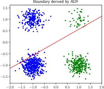
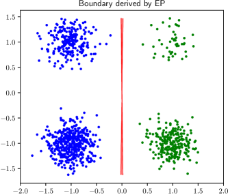
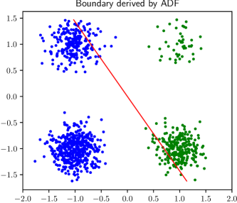
We compare EP and ADF to confirm that EP does not depend on data permutation. We generate a toy dataset in the following way: 1000 data points $x$ are generated from Gaussian mixture model $0.05N(x;[1,1],0.05I)+0.25N(x;[-1,1],0.05I)+0.45N(x;[-1,-1],0.05I)+0.25N(x;[1,-1],0.05I)$, where $N(x;\mu,\Sigma)$ denotes the Gaussian density with respect to $x$ with mean $\mu$ and covariance matrix $\Sigma$, and $I$ is the identity matrix. For $x$, we assign label $y=+1$ when $x$ comes from $N(x;[1,1],0.05I)$ or $N(x;[1,-1],0.05I)$ and label $y=-1$ when $x$ comes from $N(x;[-1,1],0.05I)$ or $N(x;[-1,-1],0.05I)$. We evaluate the dependence of the performance of BPM (see Appendix D of supplemental material for details) on the data permutation.

Figure 1: Classification boundaries derived by ADF and EP.

Fig.1 shows labeled samples by blue and green points, decision boundaries by red lines which are derived from ADF and EP for the Student-t distribution with $v=10$ by changing data permutations. The top two graph shows obvious dependence on data permutation by ADF (to clarify the dependence on data permutation, we showed the most different boundary in the figure), while the bottom graph exhibits almost no dependence on data permutations by EP.

5.2 Student-t Process Classification

We compare the robustness of Student-t process classification and Gaussian process classification.

We apply our EP method to Student-t process binary classification, where the latent function follows the Student-t process (see Appendix E of supplemental material for details). We compare this model with Gaussian process binary classification with the same likelihood term. Since the posterior distribution cannot be obtained analytically even for the Gaussian process, we use EP for the ordinary exponential family to approximate the posterior.

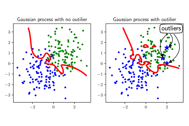
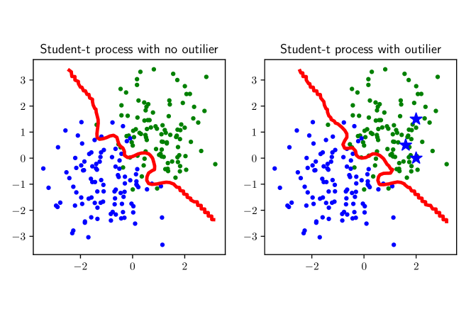
We use a two-dimensional toy dataset, where we generate a two-dimensional data point $x_{i}$ ($i=1,\ldots,200$) following the normal distribution with mean $[y_{i},y_{i}]$ and unit variance, where $y_{i}\in\{+1,-1\}$ is the class label for $x_{i}$ determined randomly. We add three outliers to the dataset and evaluate the robustness against outliers. In the experiment, we used the Gaussian kernel, and we used $v=10$ for Student-t processes.

Figure 2: Classification boundaries.

Fig.2 shows the labeled samples by blue and green points, the obtained decision boundaries by red lines, and added outliers by blue stars. As we can see, the decision boundaries obtained by the Gaussian process classifier is heavily affected by outliers, while those obtained by the Student-t process classifier are more stable. Thus, as expected, Student-t process classification is more robust against outliers compared to Gaussian process classification, thanks to the heavy-tailed structure of the Student-t distribution.

6 Conclusions

In this work, we enabled the t-exponential family to inherit the important property of the exponential family that calculation can be efficiently performed thorough natural parameters by using the q-algebra. By using this natural parameter based calculation, we developed EP for the t-exponential family by introducing the t-factorization approach. The key concept of our proposed approach is that the t-exponential family have pseudo additivity. When $t=1$, our proposed EP for the t-exponential family is reduced to the original EP for the ordinary exponential family and t-factorization yields ordinary data-dependent factorization. Therefore, our proposed EP method can be viewed as a generalization of the original EP. Through illustrative experiments, we confirmed that our proposed EP applied to the Bayes point machine can overcome the drawback of ADF, i.e., the proposed EP method is independent of data permutations. We also experimentally illustrated that our proposed EP applied to Student-t process classification exhibited high robustness to outliers compared to Gaussian process classification.

In our future work, we will further extend the proposed EP method to more general message passing methods or double-loop EP. We would like also to make our method more scalable to large datasets and develop another approximating method such as variational inference.

Appendix A Proof of Theorem 1

$$\nabla_{\theta^{\setminus j}}Z_{1} = \nabla_{\theta^{\setminus j}}\int\tilde{p}^{\backslash j}(w)l_{j}(w)^{t}dw$$

$$= \int(\phi(w)-\nabla_{\theta^{\setminus j}}g_{t}(\theta^{\setminus j}))\tilde{q}^{\backslash j}(w)l_{j}(w)^{t}dw$$

$$= \int\phi(w)\tilde{q}^{\backslash j}(w)l_{j}(w)^{t}dw-\nabla_{\theta^{\setminus j}}g_{t}(\theta^{\setminus j})\int\tilde{q}^{\backslash j}(w)l_{j}(w)^{t}dw$$

Using the definition $Z_{2}=\int\tilde{q}^{\backslash j}(w)(l_{j}(w))^{t}dw$, and $\eta=\nabla_{\theta}g_{t}(\theta)$,

$$\nabla_{\theta^{\setminus j}}Z_{1} = \eta Z_{2}-\eta^{\setminus j}Z_{2}$$

Therefore,

$$\eta=\eta^{\setminus j}+\frac{1}{Z_{2}}\nabla_{\theta^{\setminus j}}Z_{1}.$$

Appendix B Proof of Theorem 2

Here, we consider a one-dimensional case, but we can consider this in the same way as for a multivariate case. Considering the unnormalized t-exponential family, $\exp_{t}(\langle\Phi(w),\theta\rangle-g)$, and $g$ is a constant, not a true log partition function. We integrate this expression as follows,

$$\int^{\infty}_{-\infty}\exp_{t}(\langle\Phi(w),\theta\rangle-g)dw = \int^{\infty}_{-\infty}(1+\Psi(-2\mu^{\top}Kw+w^{\top}Kw)-(1-t)g)^{\frac{1}{1-t}}dw$$

$$= \int^{\infty}_{-\infty}(1-\Psi\mu^{\top}K\mu-(1-t)g+\Psi(w-\mu)^{\top}K(w-\mu))^{\frac{1}{1-t}}dw$$

$$= (1-\Psi\mu^{\top}K\mu-(1-t)g)^{\frac{1}{1-t}}\int^{\infty}_{-\infty}\Bigl{(}1+\frac{\Psi(x-\mu)^{\top}K(x-\mu)}{1-\Psi\mu^{\top}K\mu-(1-t)g}\Bigr{)}^{\frac{1}{1-t}}dw$$

Here, for simplicity, we put $(1-\Psi\mu^{\top}K\mu-(1-t)g)=A$, and use the formula, $\int^{\infty}_{0}\frac{x^{m}}{(1+x^{2})^{n}}dx=\frac{1}{2}B\bigl{(}\frac{2n-m-1}{2},\frac{m+1}{2}\bigr{)}$, where $B$ denote the beta function. We can get the expression,

$$\int^{\infty}_{-\infty}\exp_{t}(\langle\Phi(w),\theta\rangle-g)dw = \frac{1}{2}B\Bigl{(}\frac{3-t}{2(t-1)},\frac{1}{2}\Bigr{)}\Bigl{(}\frac{\Psi}{A}K\Bigr{)}^{-\frac{1}{2}}A^{\frac{1}{1-t}}$$

We can proceed with the calculation by using the definition of $\Psi$, $B(x,y)=\frac{\Gamma(x)\Gamma(y)}{\Gamma(x+y)}$, and$\Gamma(\frac{1}{2})=\sqrt{\pi}$ as follows,

$$\int^{\infty}_{-\infty}\exp_{t}(\langle\Phi(w),\theta\rangle-g)dw = \Psi^{-\bigl{(}\frac{1}{2}+\frac{1}{1-t}\bigr{)}}A^{\frac{1}{2}+\frac{1}{1-t}}$$

Here, by using the definition of $A$ and the true log partition function $g_{t}(\theta)=\frac{1}{1-t}\bigl{(}1-\Psi(\mu^{\top}K\mu+1)\bigr{)}$,

$$A^{\frac{1}{2}+\frac{1}{1-t}} = (1-\Psi\mu^{\top}K\mu-(1-t)g)^{\frac{1}{2}+\frac{1}{1-t}}$$

$$= (\Psi+(1-t)(g_{t}(\theta)-g))^{\frac{1}{2}+\frac{1}{1-t}}$$

$$= \Psi^{\frac{1}{2}+\frac{1}{1-t}}(1+(1-t)(g_{t}(\theta)-g)/\Psi)^{\frac{1}{2}+\frac{1}{1-t}}$$

Therefore, by substituting this expression into the above integral result, we get the following.

$$\int^{\infty}_{-\infty}\exp_{t}(\langle\Phi(w),\theta\rangle-g)dw=\Bigl{(}\exp_{t}(g_{t}(\theta)/\Psi-g/\Psi)\Bigr{)}^{\frac{3-t}{2}}$$

Appendix C Deriving the Marginal likelihood

$$Z_{\rm{EP}} = \int p^{(0)}(w)\otimes_{t}\prod_{i}\otimes_{t}\tilde{l}_{i}(w)dw$$

$$= \int\exp_{t}\Bigl{(}\sum_{i}\log_{t}\tilde{C}_{i}+\langle\Phi(w),\theta\rangle-g_{t}^{\rm{prior}}(\theta)\Bigr{)}dw$$

$$= \Biggl{(}\exp_{t}\Bigl{(}\sum_{i}\log_{t}\tilde{C}_{i}/\Psi+g_{t}(\theta)/\Psi-g_{t}^{\rm{prior}}(\theta)/\Psi\Bigr{)}\Biggr{)}^{\frac{3-t}{2}}.$$

Appendix D Bayes Point Machine

In this section, we show the details of the update rule of ADF and EP for the Bayes point machine.

D.1 ADF update rule for BPM

The detailed update rules of ADF for BPM in t-exponential family are derived in [6].

$$\mu^{i} = E_{q}[w]=\mu^{i-1}+\alpha y_{i}\Sigma^{i-1}x_{i}$$ (41)

$$\Sigma^{i} = E_{q}[ww^{\top}]-E_{q}[w]E_{q}[w^{\top}]=r\Sigma^{i-1}-(\Sigma^{i-1}x_{i})\biggl{(}\frac{\alpha y_{i}\langle x_{i},\mu^{i}\rangle}{x_{i}^{\top}\Sigma^{i-1}x_{i}}\biggr{)}(\Sigma^{i-1}x_{i})^{\top},$$ (42)

where $\tilde{q}_{i}(w)\propto\tilde{p}_{i}(w)^{t}$, $q_{i}(w)\propto\tilde{p}_{i-1}(w)^{t}(l_{i}(w))^{t}$, and

$$z = \frac{\alpha y_{i}\langle x_{i},\mu^{i-1}\rangle}{\sqrt{x_{i}^{\top}\Sigma^{i-1}x_{i}}}$$ (43)

$$Z_{1} = \int\tilde{p}_{i-1}(w)(l_{i}(w))^{t}dw=\epsilon^{t}+((1-\epsilon)^{t}-\epsilon^{t})\int_{\infty}^{z}\mathrm{St}(z;0,1,v)$$ (44)

$$Z_{2} = \int\tilde{q}_{i-1}(w)(l_{i}(w))^{t}dw=\epsilon^{t}+((1-\epsilon)^{t}-\epsilon^{t})\int_{\infty}^{z}\mathrm{St}(z;0,v/(v+2),v+2)$$ (45)

$$r = \frac{Z_{1}}{Z_{2}}$$ (46)

$$\alpha = \frac{((1-\epsilon)^{t}-\epsilon^{t})\mathrm{St}(z;0,1,v)}{Z_{2}\sqrt{x_{i}^{\top}\Sigma^{i-1}x_{i}}}$$ (47)

D.2 EP update rule for BPM

As for the EP update rule, natural parameters of Student-t distribution $\mathrm{St}(w;v,\mu,\Sigma)$ is $[\theta_{1},\theta_{2}]$,

$$\theta_{1} = -2\frac{\Psi K\mu}{1-t}$$ (48)

$$\theta_{2} = \frac{\Psi K}{1-t}$$ (49)

where, $K=(v\Sigma)^{-1}$. From these, we can calculate EP update rules through $\Psi K\mu$ and $\Psi K$.

For the BPM, we consider that the whole approximation is $k$-dimensional $\mathrm{St}(w;m_{w},V_{w},v)$, and the site approximation as one-dimensional Student-t like function, $\exp_{t}(\langle\Phi(w),\theta\rangle)$, where $\langle\Phi(w),\theta\rangle=\frac{\Psi_{i}}{1-t}\bigl{(}(w^{\top}x_{i})^{\top}(v\sigma_{i})^{-1}(w^{\top}x_{i})-2m_{i}(\tilde{v}\sigma_{i})^{-1}(w^{\top}x_{i})\bigr{)}\propto\frac{\Psi_{i}}{1-t}\tilde{v}^{-1}\sigma_{i}^{-1}(w^{\top}x_{i}-m_{i})^{2}$.

Note that the whole posterior approximation is the $k$-dimensional, but the site approximation is the one-dimensional, therefore the degree of freedom are different from the total approximation and the site approximation to make $t$ consistent. The relation between $v$, $\tilde{v}$, and $t$ is given as

$$\frac{1}{t-1}=\frac{v+k}{2}=\frac{\tilde{v}+1}{2}.$$ (50)

We denote the $\Psi$ and $K$ which is related to site $i$ as $\Psi_{i}$ and $K_{i}$. Since $\sigma_{i}$ is scalar, $K_{i}=(\tilde{v}\sigma_{i})^{-1}$. When we denote $\Psi=(\alpha/|\Sigma|^{1/2})^{1-t}$, then $\Psi_{i}=(\alpha_{i}/\sigma_{i}^{1/2})^{1-t}$. We denote $\Psi$ and $K$ of whole approximation as $\Psi_{w}$ and $K_{w}$.

Let us consider the update of site $j$. The first step is calculation of cavity distribution, which can be done by

$$\Psi^{\setminus j}K^{\setminus j} = \Psi_{w}(vV_{w})^{-1}-\Psi_{j}(\tilde{v}\sigma_{i})^{-1}x_{j}x_{j}^{\top},$$ (51)

$$\Psi^{\setminus j}K^{\setminus j}m^{\setminus j} = \Psi_{w}(vV_{w})^{-1}m_{w}-\Psi_{j}(\tilde{v}\sigma_{i})^{-1}m_{j}x_{j}.$$ (52)

Next step is moment matching. This is calculated in the same way as the ADF update rules. To use the ADF update rule, we have to convert $\Psi^{\setminus j}K^{\setminus j}$ and $\Psi^{\setminus j}K^{\setminus j}m^{\setminus j}$ to $V^{\setminus j}$ and $m^{\setminus j}$, which are covariance matrix and mean of cavity distribution. When calculating $V^{\setminus j}$ from $\Psi^{\setminus j}K^{\setminus j}$, we have to be careful that $\Psi^{\setminus j}$ contains the determinant of $V^{\setminus j}$. From the definition,

$$\Psi^{\setminus j}K^{\setminus j}=\Bigl{(}\frac{\alpha_{j}}{|V^{\setminus j}|^{1/2}}\Bigr{)}^{1-t}(vV^{\setminus j})^{-1}.$$ (53)

Since $\alpha_{j}$ and $v$ is the constant, when we put $\frac{{V^{\setminus j}}^{-1}}{|V^{\setminus j}|^{(1-t)/2}}=B$, following relation holds,

$$|V^{\setminus j}|=\Bigl{(}|B|^{\frac{1}{k}}\Bigr{)}^{\frac{1}{\frac{t-1}{2}-\frac{1}{k}}}.$$ (54)

Using this relation, we get $V^{\setminus j}$ and $m^{\setminus j}$.

After moment matching, we get $V_{\mathrm{new}}$ and $m_{\mathrm{new}}$. Next step is the exclusion step of site other than $j$. This step is calculated in the same way as the step of cavity distribution.

$$\Psi_{j}K_{j} = \Psi_{\mathrm{new}}K_{\mathrm{new}}-\Psi^{\setminus j}K^{\setminus j},$$ (55)

$$\Psi_{j}K_{j}\tilde{m_{j}} = \Psi_{\mathrm{new}}K_{\mathrm{new}}m_{\mathrm{new}}-\Psi^{\setminus j}K^{\setminus j}m^{\setminus j}.$$ (56)

To update site parameters, we have to convert $\Psi_{j}K_{j}$ and $\Psi_{j}K_{j}\tilde{m_{j}}$ into $\sigma_{j}$ and $m_{j}$, which are scalar values. This can be done easily by using the fact that $K_{j}$ is proportional to $\sigma_{j}^{-1}x_{j}x_{j}^{\top}$.

These steps are the update rules for the site approximation. We have to iterate these steps until site parameters converge.

Appendix E Expectation Propagation for Student-t Process Classification

In this section, we show the details of the derivation of EP for the Student-t process classification. The derivation procedure is similar to that of the Gaussian process [2][11][12][13][14].

E.1 Deriving Update Rules for Student-t Process Classification

In this subsection, we show the detailed derivation of the update rules for the Student-t process classification. We denote the prior as $p(f|X)$. In the case of Gaussian process, the prior distribution is a Gaussian distribution whose covariance is specified by the kernel function. In this case, the prior distribution is a Student-t distribution which is specified by the covariance kernel $k(x,x)$ and the degree of freedom $v$. The posterior distribution is given by $p(f|X,y)=\frac{1}{Z}p(f|X)\prod_{i}p(y_{i}|f_{i})$, where the marginal likelihood is given as $Z=p(y|X)=\int p(f|X)\prod_{i}P(y_{i}|f_{i})df$ for the i.i.d. situation. In this paper, we consider a binary classification, therefore we use

$$p(y_{i}|f_{i})=l_{i}(f_{i})=\epsilon+(1-2\epsilon)\Theta(y_{i}f_{i}).$$ (57)

This is actually the same as BPM, where the input to step function is given as a linear model. In the Student-t process, the input is given as the nonlinear probabilistic process. In this setting, the posterior is intractable; therefore, we have to approximate it.

Following the EP framework, we approximate the posterior by factorizing the posterior in terms of data. To do so, we denote the factorizing term that corresponds to data $i$ as follows.

$$\tilde{l}_{i}(f_{i}|\tilde{C}_{i},\tilde{\mu}_{i},\tilde{\sigma}^{2}_{i}):=\tilde{C}_{i}\otimes\mathrm{St}(f_{i};\tilde{\mu}_{i},\tilde{\sigma}^{2}_{i},\tilde{v})$$ (58)

For simplicity, we denote the unnormalized Student-t like function as $\mathrm{St}(f_{i};\tilde{\mu}_{i},\tilde{\sigma}^{2}_{i},\tilde{v})$. This is equivalent to $\exp_{t}(\langle\Phi(f_{i}),\theta\rangle)$, where $\langle\Phi(f_{i}),\theta\rangle=\frac{\Psi_{i}}{1-t}(f_{i}^{\top}K_{i}f_{i}-2\tilde{\mu}_{i}^{\top}K_{i}f_{i})=\frac{\Psi_{i}}{1-t}(f_{i}^{\top}(v\tilde{\sigma}_{i})^{-1}f_{i}-2\tilde{\mu}_{i}^{\top}(v\tilde{\sigma}_{i})^{-1}f_{i})$. These data corresponding factorizing terms are one-dimensional. Note that the whole posterior approximation is the $k$-dimensional, but site approximation is the one dimensional, the same relation as in the BPM between $v$, $\tilde{v}$, and $t$ holds as $\frac{1}{t-1}=\frac{v+k}{2}=\frac{\tilde{v}+1}{2}$.

The q products of this data corresponding term can be expressed as follows:

$$\prod_{i}\otimes_{t}\tilde{l}_{i}(f_{i})=\mathrm{St}(\tilde{\mu},\tilde{\Sigma},v)\otimes_{t}\prod_{i}\otimes_{t}\tilde{C}_{i}$$ (59)

Here, we used the property that q products of Student-t distribution become a Student-t distribution. In the above expression, $\tilde{\mu}$ is the vector of $\tilde{\mu}_{i}$ and $\tilde{\Sigma}$ is the diagonal and following relations are given,

$$\tilde{K}^{-1} = (v\tilde{\Sigma}),$$ (60)

$$\tilde{\Psi}\tilde{K} = \rm{diag}(\Psi_{1}K_{1}\dots\Psi_{n}K_{n}),$$ (61)

$${\rm where\ \ }\tilde{\Psi}=\Biggl{(}\frac{\Gamma((v+k)/2)}{(\pi v)^{k/2}\Gamma(v/2)|\tilde{\Sigma}|^{1/2}}.\Biggr{)}^{1-t}.$$ (62)

Therefore, the total form of the approximation of the posterior can be expressed as follows.

$$q(f|X,y)=\mathrm{St}(\mu,\Sigma,v)\propto p(f|X)\otimes_{t}\Bigl{(}\prod_{i}\otimes_{t}\tilde{l}_{i}(f_{i})\Bigr{)}$$ (63)

From this following relations are obtained,

$$\Psi K=\Psi_{0}K_{0}+\tilde{\Psi}\tilde{K},$$ (64)

$$\Psi K\mu=\tilde{\Psi}\tilde{K}\tilde{\mu}.$$ (65)

We consider the case that we update site $i$. For implementation, natural parameter based update rule is preferable. Therefore we define the parameter as follows,

$$\tilde{\tau}_{i}=\tilde{\Psi}_{i}\tilde{K}_{i},$$ (66)

which is the (i,i) element of $\tilde{\Psi}\tilde{K}$. We also define,

$$\tilde{\nu}_{i}=\tilde{\Psi}_{i}\tilde{K}_{i}\tilde{\mu}_{i}.$$ (67)

For the cavity distribution, we define in the same way as,

$$\tau_{-i} = \Psi_{-i}\sigma_{-i}^{-2}\tilde{v}^{-1},$$ (68)

$$\nu_{-i} = \tau_{-i}\mu_{-i}.$$ (69)

The first step is to calculate the cavity distribution, we eliminate the effect of site $i$. To do so, we first integrate out non $i$ terms by using the following formula. Let X and Y are random variable that obey the Student-t distribution,

$$\left(\begin{array}[]{r}X\\ Y\end{array}\right)\sim\mathrm{St}\Biggl{(}\left(\begin{array}[]{r}\mu_{x}\\ \mu_{y}\end{array}\right),\left(\begin{array}[]{rr}\Sigma_{xx}&\Sigma_{xy}\\ \Sigma_{yx}&\Sigma_{yy}\end{array}\right),v\Biggr{)}.$$ (76)

The marginal distribution X is given as,

$$X\sim\mathrm{St}\bigl{(}\mu_{x},\Sigma_{xx},v\bigr{)}$$ (77)

By utilizing the above formula, we get

$$q_{-i}(f_{i}) \propto \int p(f|X)\otimes_{t}\prod_{j\neq i}\otimes_{t}l_{j}(f_{j})df_{j}$$ (78)

$$\propto \mathrm{St}(\mu_{i},\sigma^{2}_{i},v).$$ (79)

where, $\mu_{i}$ is the $i$th element of $\mu$ and $\sigma^{2}_{i}$ is the $(i,i)$ element of $\Sigma$. In the above expression, the degree of freedom is $v$ in both the joint distribution and marginal distribution. This is unfavorable for our Student-t process. To make the EP procedure consistent with $t$, we approximate as $q_{-i}(f_{i})\propto\mathrm{St}(\mu_{i},\sigma^{\prime 2}_{i},\tilde{v})$, $\sigma^{\prime 2}_{i}=\sigma^{2}_{i}v/\tilde{v}$. Since for a one-dimensional Student-t distribution, its variance is given by $(v\sigma^{2}_{i})^{-1}$, and in this case, $\tilde{v}>v$, approximation by $\sigma^{\prime 2}_{i}=\sigma^{2}_{i}$ would result in the underestimate of the variance.

We calculate the cavity distribution in the following way,

$$\tau_{-i} = \tilde{v}^{-1}{\sigma^{\prime}}_{i}^{-2}\Psi_{i}-\tilde{\tau}_{i},$$ (80)

$$\nu_{-i} = \tilde{v}^{-1}{\sigma^{\prime}}_{i}^{-2}\Psi_{i}\mu_{i}-\tilde{\nu}_{i}.$$ (81)

Next step is the inclusion of data $i$ to the approximate posterior. This can be done in the same way of BPM. To derive the update rule, we have to convert $\tau_{-i}$ and $\nu_{-i}$ into $\sigma^{2}_{-i}$ and $\mu_{-i}$. In this case, the site approximations are one-dimensional, following relation holds,

$$\hat{\mu}_{i} = \mu_{-i}+\sigma^{2}_{-i}\alpha,$$ (82)

$$\hat{\sigma_{i}^{2}} = \sigma^{2}_{-i}(r-\alpha\hat{\mu}_{i}),$$ (83)

$$\ \ \ \mathrm{where}\ \ \alpha=\frac{\bigl{(}(1-\epsilon)^{t}-\epsilon^{t}\bigr{)}\mathrm{St}(z:,0,1,\tilde{v})}{Z_{2}\sqrt{\sigma^{2}_{-i}}}\ \mathrm{and}\ \ z=\frac{y_{i}\mu_{-i}}{\sqrt{\sigma^{2}_{-i}}},$$ (84)

where the definition of $Z_{2}$ and $r$ is same as that of BPM. By using $\sigma^{2}_{-i}$ and $\mu_{-i}$, we can include the data $i$ information.

After the data inclusion step, we exclude the effect other than data $i$. The calculation of this step can be done in the same way as that of cavity distribution,

$$\tilde{\tau}_{i}^{\mathrm{new}} = \tilde{v}^{-1}\hat{\sigma}_{i}^{-2}\hat{\Psi}_{i}-\tilde{\tau}_{-i},$$ (85)

$$\tilde{\nu}_{i}^{\mathrm{new}} = \tilde{v}^{-1}\hat{\sigma}_{i}^{-2}\hat{\Psi}_{i}\hat{\mu}_{i}-\tilde{\nu}_{-i}.$$ (86)

From this $\tilde{\tau}_{i}^{\mathrm{new}}$, we can update $\tilde{\Psi}\tilde{K}$. Since $\tilde{\Psi}\tilde{K}$ is the diagonal matrix, we just update $(i,i)$ element of $\tilde{\Psi}\tilde{K}$.

As a final step, we have to update $\Sigma$. To circumvent the calculation of inverse matrix, we put

$$\Delta\tau=-\tilde{\tau}_{i}^{\mathrm{new}}-\tilde{\tau}_{-i}+\tilde{v}^{-1}\hat{\sigma}_{i}^{-2}\hat{\Psi}_{i}$$ (87)

From this, update of $\Psi K$ is given as,

$$\Psi^{\mathrm{new}}K^{\mathrm{new}}=\Psi^{\mathrm{old}}K^{\mathrm{old}}+\Delta\tau e_{i}e_{i}^{\top}$$ (88)

where $K^{\mathrm{new}}=(v\Sigma^{\mathrm{new}})^{-1}$ and $K^{\mathrm{old}}=(v\Sigma^{\mathrm{old}})^{-1}$. Here, $\Sigma^{\mathrm{new}}$ is the after the update of $\Sigma$ and $\Sigma^{\mathrm{old}}$ is the before the update of $\Sigma$ and $e_{i}$ is the unit vector of $i$ th direction. By using the matrix formula, that is, for matrix $A$ and $B$, $(A^{-1}+B^{-1})^{-1}=A-A(A+B)^{-1}A$, we can get the following expression,

$${\Psi^{-1}}^{\mathrm{new}}v\Sigma^{\mathrm{new}}={\Psi^{-1}}^{\mathrm{old}}v\Sigma^{\mathrm{old}}-\frac{\Delta\tau}{1+\Delta\tau{\Psi^{-1}}^{\mathrm{old}}v\Sigma^{\mathrm{old}}}s_{i}s_{i}^{\top},$$ (89)

where $s_{i}$ is the $i$’s column of ${\Psi^{-1}}^{\mathrm{old}}v\Sigma^{\mathrm{old}}$. From ${\Psi^{-1}}^{\mathrm{new}}v\Sigma^{\mathrm{new}}$, we can get $\Sigma^{\mathrm{new}}$.

These are the update rule of site $i$. We iterate these steps until parameters converge.

E.2 Hyperparameter Learning

In this subsection, we refer how to derive hyperparameters, such as the wave-length of covariance functions.

In the usual exponential family and Gaussian process, the hyperparameters can be derived by gradient descent for the marginal log likelihood after the EP updates end. Following the discussion in [13], we can derive almost the same expression for the gradient of $\log_{t}Z_{\rm{EP}}^{\frac{2}{3-t}}$. When we consider the gradient of hyperparameter $\psi_{i}$,

$$\frac{\partial\log_{t}Z_{\rm{EP}}^{\frac{2}{3-t}}}{\partial\psi_{j}}=\eta^{\top}\frac{\partial\theta_{prior}}{\partial\psi_{j}}-\eta^{\top}_{prior}\frac{\partial\theta_{prior}}{\partial\psi_{j}}+\sum_{i}\frac{\partial\log_{t}\tilde{C}_{i}}{\partial\psi_{j}}$$ (90)

where, $\theta_{\rm{prior}}$ is the natural parameters of prior distribution and $\eta_{\rm{prior}}$ is the expected sufficient statistics of the prior distribution.

E.3 Prediction Rule

In this subsection, we refer to the method of deriving the prediction for the Student-t process classification. After the EP updates end, we have the analytic expression of the approximate posterior distribution as $q(f|X,y)=\mathrm{St}(\mu,\Sigma,v)$.

When a new point $x^{*}$ is given, we would like to predict its label $y^{*}$. First we calculate the latent variable $f^{*}$ of $x^{*}$. To get the expression of $f^{*}$, we use the following lemma in [4],

Lemma 1

If $X\sim\mathrm{St}(\mu,\Sigma,v)$, and $x_{1}\in R^{n_{1}}$, $x_{2}\in R^{n_{2}}$ express the first $n_{1}$ and remaining $n_{2}$ entries of X respectively. Then

$$x_{2}|x_{1}\sim\mathrm{St}\Bigl{(}\tilde{\mu}_{2},\frac{v+\beta_{1}}{v+n_{1}}\times\tilde{\Sigma}_{22},v+n_{1}\Bigr{)},$$ (91)

where $\tilde{\mu}_{2}=\Sigma_{21}\Sigma_{11}^{-1}(x_{1}-\mu_{1})+\mu_{1}$, $\tilde{\Sigma}_{22}=\Sigma_{22}-\Sigma_{21}\Sigma_{11}^{-1}\Sigma_{12}$, $\beta_{1}=(x_{1}-\mu_{1})^{\top}K_{11}^{-1}(x_{1}-\mu_{1})$.

We consider the following expression,

$$p(\tilde{f}|X,x^{*})=\int p(\tilde{f}|f,x^{*})p(f|X)df.$$ (92)

The mean of $p(\tilde{f}|X,x^{*})$ is given by

$$\mathrm{E}[\tilde{f}] = \int\mathrm{E}[p(\tilde{f}|f,x^{*})]p(f|X)df$$ (93)

$$= \int k^{\top}\Sigma^{-1}fp(f|X)df$$ (94)

$$= k^{\top}\Sigma^{-1}\mu$$ (95)

where, $k=[k(x^{*},x_{1}),\dots k(x^{*},x_{n})]^{\top}$. Therefore strict classification of $x^{*}$ is given by

$$\mathrm{sign}\bigl{(}\mathrm{E}[\tilde{f}]\bigr{)}=\mathrm{sign}\bigl{(}k^{\top}\Sigma^{-1}\mu)$$ (96)

Using this expression, we get the decision boundary.

References

• [1] C. M. Bishop: Pattern Recognition and Machine Learning. Springer,2006
• [2] C. E. Rasmussen and C.K.I. Williams: Gaussian Processes for Machine Learning. The MIT Press,2006
• [3] P. Jylanki, J. Vanhatalo, and A. Vehtari: Robust Gaussian Process Regression with a Student-t Likelihood. The Journal of Machine Learning Research,12, 3227-3257,2011
• [4] A. Shah, A. Wilson, and Z. Ghahramani: Student-t Processes as Alternatives to Gaussian Processes. Proceedings of the 17th International Conference on Artificial Intelligence and Statistics,2014
• [5] N. Ding and S.v.n. Vishwanathan: t-logistic regression. Advances in Neural Information Processing Systems 23,2010
• [6] N. Ding and Qi, Yuan and S.v.n. Vishwanathan: t-divergence Based Approximate Inference. Advances in Neural Information Processing Systems 24,2011
• [7] M. Seeger: Expectation Propagation for Exponential Families. Technical Report, Department of EECS, University of California, Berkeley,2006
• [8] L. Nivanen, A. Le Mehaute, and Q. A. Wang: Generalized Algebra within a Nonextensive statistics. Rep. Math. Phys. 52, 437-434,2003
• [9] H. Suyari and M. Tsukada: Law of Error in Tsallis Statistics. IEEE Trans. Inform. Theory, 51, 753-757,2005
• [10] T. Minka: Expectation Propagation for Approximative Bayesian Inference. PhD thesis, MIT Media Labs, Cambridge, USA,2001
• [11] Y. Li, J. Hern’andez-Lobato, and R. Turner: Stochastic Expectation Propagation. Advances in Neural Information Processing Systems 28,2015
• [12] H. Nickisch and C. E. Rasmussen: Approximations for Binary Gaussian Process Classification. Journal of Machine Learning Research, 9, 2035–2078,2008
• [13] D. Hern’andez-Lobato and J. M. Hern’andez-Lobato: Scalable Gaussian Process Classification via Expectation Propagation. 19th International Conference on Artificial Intelligence and Statistics,2016
• [14] M. Kuss and C. E. Rasmussen: Assessing Approximate Inference for Binary Gaussian Process Classification. Journal of Machine Learning Research, 6, 1679–1704,2005