A nested sampling code for targeted searches for continuous gravitational waves from pulsars
Abstract
This document describes a code to perform parameter estimation and model selection in targeted searches for continuous gravitational waves from known pulsars using data from ground-based gravitational wave detectors. We describe the general workings of the code and characterise it on simulated data containing both noise and simulated signals. We also show how it performs compared to a previous MCMC and grid-based approach to signal parameter estimation. Details how to run the code in a variety of cases are provided in Appendix A.
01.50.ht, 02.50.Tt, 04.80.Nn \preprint
1. Overview
There are a variety of sources of gravitational waves that are potentially observable using the current ground-based gravitational wave detectors (Aasi et al., 2015; Acernese et al., 2015). These include transient signals, such as those already observed from the merger of binary black hole systems (Abbott et al., 2016a, b), and also continuous quasi-monochromatic signals, such as expected from assymetrically deformed rotating neutron stars (see, e.g., Section III of Abbott et al., 2004). Here we will describe a code used in searches for continuous gravitational wave signals, in particular signals from sources that are seen as pulsars via electromagnetic observations.
One of the primary methods used in searches for gravitational waves from known pulsars is based on two stages: a heterodyne stage that pre-processes the calibrated gravitational wave detector data by removing a signal’s expected intrinsic phase evolution (based on the observed solution from electromagnetic observations), whilst also low-pass filtering and down-sampling (via averaging) the heterodyned data (Dupuis and Woan, 2005); and, a parameter estimation stage that takes the processed data and uses it to estimate posterior probability distributions of the unknown signal parameters (e.g., using a Markov chain Monte Carlo (MCMC) Abbott et al., 2010). This method has been variously called the Time Domain Method, the Heterodyne Method, the Bayesian Method, the Glasgow Method, or some combination of these names. Up to now this method has only been used to set upper limits on signal amplitudes, but has included no explicit criteria for deciding on signal detection/significance. A further limitation has been that the MCMC method used was inefficient111MCMC methods are not intrinsically inefficient for searches such as our, but the particulat implementation we had used was not specically designed to be efficient at sampling the given posterior volumes. and required a lot of tuning. It also did not straightforwardly have the ability to perform a search on the data over small ranges in the phase evolution parameters, which is required if the gravitational wave signal does not well match the known pulsar’s phase evolution. A nested sampling algorithm (Skilling, 2006), in particular a method based on that described in Veitch and Vecchio (2010), has been provided within the LALInference software library (Veitch et al., 2015) in LIGO Scientific Collaboration (2017). This has been used for parameter estimation and model selection for both modelled transient sources, such as the observed black hole mergers (Abbott et al., 2016c), and unmodelled transient signal searches (Lynch et al., 2015). Due to the above reasons, and to make use of the existing and well used library functions, the code has been re-written to use the available nested sampling algorithm. This allows us to evaluate the evidence or marginal likelihood for the signal model and compare it to other model evidences (i.e. the data is consistent with being just Gaussian noise), whilst also giving posterior probability distributions for the signal parameters.
This code is called lalapps_pulsar_parameter_estimation_nested (or lppen for short through the rest of this document). For more detailed descriptions of how the algorithm works we refer to Veitch and Vecchio (2010) and (Veitch et al., 2015), whilst here we will provide some information on the specific proposal distributions that can be used within the algorithm. This method has previously been briefly described in Pitkin et al. (2012). The previous code, called lalapps_pulsar_parameter_estimation (or lppe for short), used in, e.g., Abbott et al. (2010), could perform posterior evaluation using two methods: an MCMC method, or, by gridding up the parameter space and explicitly evaluating the posterior at each grid point. In §4 we show comparisons of the various methods mainly to check lppen for consistency.
The code can also be used to perform parameter estimation and model selection for signals for any generic metric theory of gravity, however its use for this is discussed in more detail in a separate paper (Isi et al., 2017). When searching over parameters that vary the phase evolution there is potential to speed up the analysis through efficient likelihood evaluation via the reduced order quadrature method (see, e.g., Field et al., 2014; Canizares et al., 2015), but again that will be discussed in more detail in a future paper.
1.1. Background knowledge
The code calculates the Bayesian evidence, or marginal likelihood, for a particular signal model under a set of assumptions. The evidence, , for a given model, , defined by a set of parameters, , is given by
| (1) |
where is the likelihood function for the data given the model and its set of defining parameters, is the prior probability distribution on , and represents any additional prior assumptions. During nested sampling this integral is evaluated by transforming it into the one dimensional sum
| (2) |
where is the “prior weight” (i.e. the fraction of the prior occupied by point ).
By default the signal model evidence is compared to the evidence that the data consists of only Gaussian noise to form the odds for the two models
| (3) |
where on the right hand side we have explicitly set the prior odds for the two models to .
Other than this evidence value and odds, the code also returns the samples accumulated during the nested sampling process. These samples are not drawn from the posterior probability distribution as in an MCMC method, but they can be resampled to generate a subset of samples that are drawn from the posterior distribution. This resampling (performed using the lalapps_nest2pos python script within lalapps LIGO Scientific Collaboration, 2017) uses the value of for each point, normalised by , to give values proportional to the posterior probability, and then accepts a point with a probability given by its value, i.e. a point is accepted with the probability
| (4) |
In our case the data in equation 1.1 is the heterodyned, low-pass filtered and down-sampled data from a detector, or set of detectors, each giving a single data stream or two data streams depending on whether the heterodyne was performed at one or both potential signal frequencies near the rotation frequency and/or twice the rotation frequency. Here we will use to represent a vector of these heterodyned data values (Dupuis and Woan, 2005), for which a single time sample is often referred to using the jargon term (“B of k”), although we will not consistently use as the time index for the data. Throughout this document if we refer to “heterodyned” data we mean data that has been processed, or simulated as if processed, by this method.
2. Core functions
Here we will describe the core parts of the code defining the signal model and the probability functions used for the inference. These assume that the data comprises a number of calibrated narrow-band complex-heteroyned time series. These time series data streams can be from different detectors, and/or at different heterodyne frequencies. For example you could have a pair of times series from both the LIGO Hanford (H1) and LIGO Livingston (L1) detectors, with each pair containing one produced with a heterodyne at twice the rotation frequency of a known pulsar and the other produced with a heterodyne at the rotation frequency.
2.1. The signal model
Our code assumes that the electromagnetically observed rotational phase evolution of a pulsar is represented by its Taylor expansion
| (5) |
where is the time, corrected to an inertial reference frame (the solar system barycentre for isolated pulsars, or the binary system barycentre for pulsars in binaries or multiple component systems), and the ’s give the observed rotation frequency and its time derivatives. The value of where is the time at a detector, is the time dependent correction to the inertial frame and is the epoch. The code can accept frequency derivatives of any order. We assume the calibrated detector data, , has been heterodyned such that
| (6) |
where is the assumed phase evolution for a given data stream , and we produce by low-pass filtering and resampling (via averaging) values of .
Under the standard assumption that the general theory of relativity (GR) is correct, the code uses the most general form of the signal model defined in Equations 51–54 of Jones (2015), which, when heterodyned and assuming low-pass filtering, gives a signal at a pulsar’s rotation frequency (where ) of {widetext}
| (7) |
and at twice the pulsar’s rotation frequency (where ) of
| (8) |
The and values are the detector () dependent antenna patterns (see, e.g., Forward (1978); Schutz and Tinto (1987); Finn (2009), or Jaranowski et al. (1998) for the convention used within this document in, e.g., equation 2.2.4), which are a function of the detector position, source sky position and source polarisation angle (in equations 7 and 8 we only explicitly note the dependence as for our sources the sky location is known). The , , and values are convenient ways of representing the waveform in terms of an amplitude and phase of the signal for the , harmonic and harmonic respectively. The values represent any time dependent phase deviation between the phase used in the heterodyne and the true signal phase (which does not necessarily have to precisely follow the electromagnetically observed rotational phase, see discussions in, e.g., Abbott et al., 2008), so and . More generally, for emission at an arbitrary scaling of the rotation frequency, (where ), an even more generic signal model (still assuming GR is correct) would be
| (9) |
where and are the amplitude components for the ‘’ and ‘’ polarisations, and is the signal’s initial phase.
To calculate the values using up to the frequency derivative, and to avoid numerical overflow issues when dealing with large phases, we use {widetext}
| (10) |
where is the frequency derivative (for both the ‘true’ and ‘het’ the frequency/frequency dervitative values used here are those prior to scaling by for a given signal model), and is the combination of any solar system barycentring and binary system barycentring time delays.
By default the code assumes emission just from the mode, i.e. there is only a signal at twice the rotation frequency. In this case and can be related to the more familiar physical and values via (where the minus sign maintains consistency of equation 8 with the form given in Jaranowski et al., 1998) and pulsar rotational phase . For the more general case the relations between the waveform amplitude and phase parameters and physical source parameters are given in Jones (2015) and Pitkin et al. (2015). In general, for previous searches we have often assumed that we track the true signal phase perfectly with the heterodyne, and as such . In such cases the only time varying components of the signal are the antenna pattern functions, which allows great speed increases in the signal generation and likelihood calculations (see §2.2.4).
2.1.1 General tensor-vector-scalar signal model
A more generic heterodyned model, assuming gravity is described by an arbitrary metric theory, but not necessarily GR, is given by (see, e.g. Isi et al., 2015, 2017) {widetext}
| (11) |
where (for ) are the amplitudes for the tensor (‘’ and ‘’), vector (‘x’ and ‘y’), and scalar (‘b’ and ‘l’) gravitational wave amplitude components, are their associated time dependent antenna responses (see, e.g. Nishizawa et al., 2009; Błaut, 2012; Isi et al., 2015), and and are angles related to the initial phase of, and rotation within, the tensor, vector and scalar components. For networks of quadrupolar antennas, like a standard gravitational wave interferometer, the two scalar components are entirely degenerate (Will, 2014), and as such only one of them needs to be defined (e.g., only the ‘b’ mode is used in Equation 19 of Isi et al., 2017). When searching for a generic signal such as this the orientation of the wave-frame (given by and ) used to define the polarisation modes is arbitrary: one is free to pick any right-handed frame one wants and define the modes there, but we usually make a choice that we know simplifies things for a given signal. Hence, for a generic search, we are free to arbitrarily set our frame such that and the values given in equation 11 can be defined by, e.g., equations 24–29 of Isi et al. (2015). However, when we have a specific prediction of what a given waveform should look like, it is always in a particular frame. By convention, this is usually a frame in which the x-axis is aligned with the intersection of the equatorial plane of the source with the plane of the sky (though the convention is not universal). In other words, if a theory predicts certain amounts of polarisation with some specific phase evolution (say, that given by GR) then that is a frame dependent statement, and in required to orient the model frame accordingly. In such a case (e.g., GR or some other theory such as G4v in Mead, 2015) the antenna patterns could be obtain from those with using equations 30–35 (and and from equations 46–47, and 49–50, for GR and G4v respectively) of Isi et al. (2015) would be required.
2.2. The likelihood functions
Our code can make use of two different likelihood functions. The default is a Student’s t-likelihood function in which it is assumed that the standard deviation of the noise in the data is unknown, but can be marginalised over. A Gaussian likelihood function can also be used, for which the code can either take in estimates of the noise standard deviation at each data point, or calculate these internally based on stationary stretches of data. For the Student’s t-likelihood function, and if calculating noise standard deviations for the Gaussian likelihood function internally, the code needs to break up the data into segments for which the noise can be assumed to have been drawn from independent Gaussian distributions. The method for doing this is given in §2.4.
2.2.1 Student’s t-likelihood
A full derivation of the Student’s t-likelihood function (see, e.g., Dupuis and Woan, 2005) is given in Appendix B, but the final form of the joint likelihood (and its natural logarithm, which is actually used within the code to maintain precision) for multiple detectors and data streams is given by {widetext}
| (12) |
where is the number of detectors used, is the number of data streams (e.g., heterodyned data from both the rotation frequency and twice the rotation frequency) per detector, is the total number of independent data chunks for detector and data stream with lengths , and (with ) being the index of the first data point in each chunk. The signal model is that given by Eqns. 7 and/or 8 (or Eqn. 9) depending on which data streams are being analysed. For notational convenience we have made the substitution .
2.2.2 Gaussian likelihood
The Gaussian likelihood, and its natural logarithm, are similarly given by {widetext}
| (13) |
where is the length of each dataset and . Note that normalisation factor reflects the fact that exponential is already the product of the real and imaginary data components.
2.2.3 The null likelihood
As we will most often want to perform model comparison for the signal model against one for which the data just contains noise (the null hypothesis in this case) we can define the null likelihoods for both of the above likelihoods by setting , giving
| (14) |
for the Student’s t-likelihood, and
| (15) |
for and Gaussian likelihood.
If we were only interested in comparing models calculated using equivalent likelihood functions we could in general ignore the factors that do not depend on the data or the model, as they would cancel in any odds ratio. But, in this code we keep them for cases when such a comparison is not performed, e.g., if we want to compare the joint multi-detector likelihood for a signal with the incoherent product of likelihoods from each detector then we would need these factors to still be present.
2.2.4 Fast likelihood evaluations
In cases when the only time varying components of the model are the antenna pattern functions (i.e. when in equation 7 or 8 is zero) the likelihood evaluation can be greatly sped-up by pre-calculating the components in the internal summations. For a given sky position and detector, , and using the standard reference frame, the antenna patterns can be written as (Jaranowski et al., 1998, following the form of)
| (16) |
where is the gravitational wave polarisation angle, is the known angle between the detector arms (generally ), and and are the time dependent functions for a given detector position and source sky location that vary over a sidereal day.222The functions and are just the antenna patterns in a frame defined with . The actual definition of the antenna pattern functions is given in, e.g., Equation 23 of Isi et al. (2015). These functions can be precomputed at a set of times over a sidereal day and used, via look-up table interpolation, to give the value at any other time (our code defaults to calculate and at 2880 points over a sidereal day). However, the vast majority of the speed-up comes from pre-computing summations over the combinations of the data and the and functions. This is described in more detail in Appendix C.
In the case where we want to search over phase evolution parameters, meaning that in the model, then we cannot perform this pre-summing. However, reduced order quadrature methods (e.g. Field et al., 2014; Canizares et al., 2015) may help in these cases. Such a method is implemented in our code, but will be discussed in a separate paper.
2.3. The prior functions
An important part of any Bayesian inference method is the choice of parameter prior probability functions. Here we describe the prior functions allowed in the code for any of the required parameters.
Certain parameters are physically not allowed to take negative values, so it is hardcoded that the following parameters have zero probability below zero: gravitational wave amplitude, ; mass quadrupole moment, ; the pulsar distance; the pulsar parallax; the speed of gravitational waves; the projected semi-major axis of a binary orbit; the total binary system mass; and, the companion mass in a binary system.
There are also other hardcoded priors for waveform amplitudes in two particular cases when searching for emission at both once and twice the rotation frequency: if searching for a signal from a biaxial star then the two waveform amplitudes, and , must either both be positive or both be negative; if using the “source” model then the two amplitudes and , must have (see, e.g., Pitkin et al., 2015).
2.3.1 Uniform prior
A parameter can be given a uniform (or flat, or top-hat) prior, in which the probability is constant within a given range and zero outside that range, i.e.
| (17) |
where for parameter the upper and lower bounds on the parameter values are and . This prior can be normalised by setting , although within nested sampling the normalisation is not specifically required. The prior requires a lower and upper bound to allow it to be normalisable and to enable an initial set of samples to be drawn from it. However, it should be noted that the choice of range will have an effect on evidences that are calculated as it affects the volume of parameter space allowed by the model.
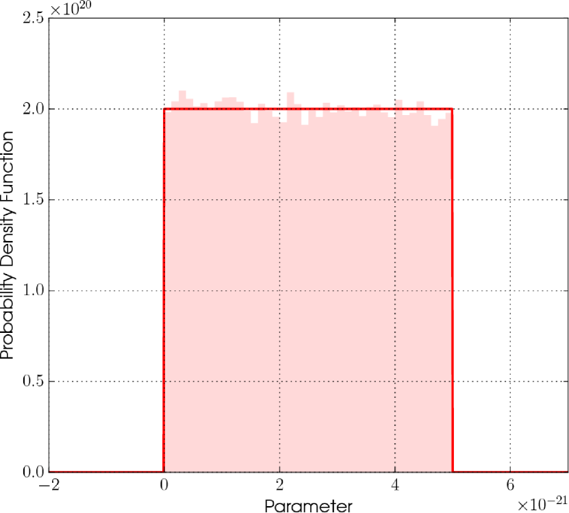
A histogram of a set of samples produced by the code when drawing from a uniform prior distribution are shown in Figure 1, along with the true prior function.
Some parameters for which the uniform prior is often considered appropriate are angle parameters, such as the and parameters in Equation 8, which can be restricted to a specific non-degenerate range (see, e.g., Table 1 in Pitkin et al., 2015). In previous gravitational wave pulsar searches, such as Abbott et al. (2010); Aasi et al. (2014) a uniform prior was often used for the gravitational wave amplitude parameter . For those searches the prior upper bound was based on inspection of the data to find a value that was very large compared to the sensitivity suggested by the data. A uniform prior was used, as opposed to the more uninformative choice for such a scale parameter of the log-uniform prior (see §2.3.4), due to the fact that the main result was in producing upper limits, and wanting these to be trivially related to the likelihood, rather than being heavily influenced by the prior.
2.3.2 Gaussian prior
A parameter can be given a prior with a Gaussian distribution, defined by its mean, , and standard deviation, , i.e.
| (18) |
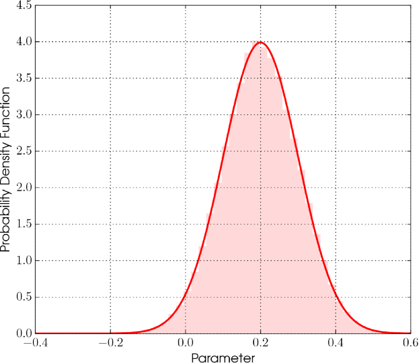
A histogram of a set of samples produced by the code when drawing from a Gaussian prior distribution are shown in Figure 2, along with the true prior function.
As well as single parameters being given Gaussian priors, we can define a set of parameters, , to have a multi-variate Gaussian prior
| (19) |
where are the means and is the covariance matrix. In reality we input the correlation coefficient matrix and individual parameter standard deviations rather than the covariance matrix, but it is easy to convert between the two.
2.3.3 Gaussian Mixture Model prior
A parameter, or any set of parameters, can be given a prior distribution composed of a superposition of Gaussian distributions (a Gaussian Mixture Model), with each component defined by a set of means for each parameter, a covariance matrix, and a weight describing the relative probability concentrated in it. For an component mixture on a set of parameters, , the prior function will be
| (20) |
where, for component , is the weight, , are the means, and is the covariance matrix.
Such a model can be used, for example, if there is a bimodal Gaussian prior on a particular parameter, as is the case for the inclination angle if it is calculated from fits to pulsar wind nebulae (see, e.g., Appendix B in Abbott et al., 2017). In such a case the Gaussian Mixture Model can define two Gaussian distributions of equal standard deviations and weights. A more complex use of this prior would be for reconstructing a smooth probability distribution using samples drawn from it, i.e. taking posterior samples from a search for a particular pulsar, and reconstructing a smooth model of those samples (for, say, the two parameters and ) to then be input as a prior when looking at future data for the same source.
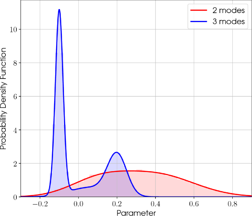
Two examples of histograms of samples drawn from one-dimensional Gaussian Mixture Models with two and three modes respectively are shown in Figure 3.
2.3.4 Log-Uniform prior
A parameter can be given a prior distribution that is uniform in the logarithm of the parameter, i.e.
| (21) |
This prior requires minimum and maximum values to be specified to make it normalisable and allow samples to be drawn from the distribution. It should be noted that the choice of range, and in particular the lower bound, will have some effect on the calculated evidence (see, e.g., Appendix B of Isi et al., 2017).
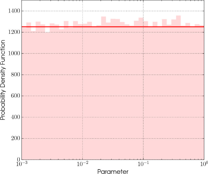
A histogram of a set of samples produced by the code when drawing from a log-uniform prior distribution, with a range between and 1 are shown in Figure 4, along with the true prior function.
2.3.5 Fermi-Dirac prior
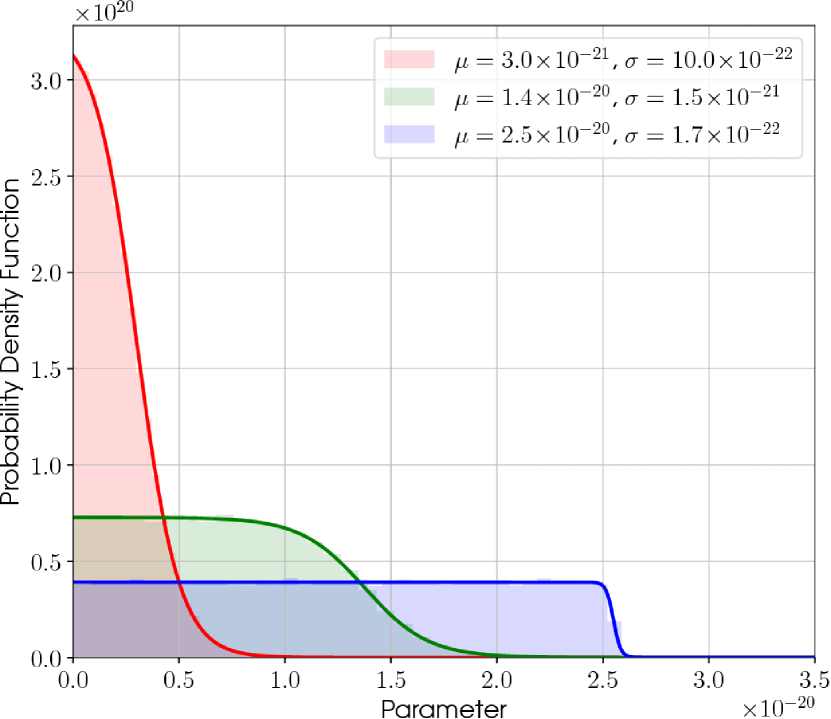
A Fermi-Dirac distribution prior function was inspired by that used in Middleton et al. (2015). The prior has a sigmoid, or logistic, shape, although starts at large values and slopes downwards and is restricted to positive values. The form of the function, for parameter , is
| (22) |
and is defined by two parameters and . defines the point at which the distribution falls to 50% of its maximum value, whilst defines the range over which the attenuation happens. We also make use of a parameter . The band over which the probability falls from 97.5% to 2.5% of its maximum value is given by , where . Therefore, if we want, for example, the distribution to have this particular fall-off over a range that is 10% of , we would have and .
Three different examples of Fermi-Dirac priors, and samples drawn from them by the code, are shown in Figure 5, for a selection of and values.
The sampling from the prior uses inverse transform sampling. The cumulative distribution function (CDF) of Equation 22 is {widetext}
| (23) |
which can be inverted to give
| (24) |
Thus, drawing CDF samples uniformly between 0 and 1, and inverting via the above equation gives values drawn from Equation 22.
This prior can use useful for amplitude parameters, where a uniform prior may have previously been used. It has the property of being roughly flat at low values of the parameter and with an exponential fall-off at large values. This gives the advantage over a uniform prior with a sharp upper cut-off in that the distribution is continuous rather than (perhaps) arbitrarily truncated.
2.4. Splitting the data
The Student’s -likelihood function (§2.2.1) requires us to have an idea about the timescales on which the data is stationary, i.e. periods when the noise in the data is best described as being drawn from a single Gaussian distribution. We therefore use a scheme similar to the BayesianBlocks change point algorithm (Scargle, 1998), or BlockNormal gravitational wave burst finding algorithm (McNabb et al., 2004), to find points at which the statistics of the noise changes. This is done with a top-down iterative divide and conquer approach (Scargle, 2000).
We start by taking a full complex time series data set for a detector and subtracting a running median from both the real and imaginary components. This subtraction is performed to try and remove the effect of any very strong signals in the data, as we want to assess the properties of the noise rather than any signal.333In reality this is only likely to be an issue for strong simulated signals injected into the data, as real signals will most likely have a low signal-to-noise ratio in short stretches of data. The running median is calculated over a running window of 30 data points (or a minimum of 15 points at the start or end of the data), but not accounting for gaps in the data. For the standard data sample rate of 1 per 60 seconds, this means that half an hour of data is used, over which time the signal (through the varying antenna patterns) will not change very much (unless there is a gap in the data). However, it should be noted that, if using a much more slowly sampled data set, then this hardcoded 30 sample window may not work well for very strong signals.
The next thing we do is calculate the evidence that the whole (running-median-removed) dataset is drawn from a single Gaussian distribution with unknown variance. To do this we just use Equation 2.2.3, with , , , and, given a dataset of length , set . We will call the natural logarithm of this value . We want to calculate the odds between this evidence and that for the data containing any single change point (i.e. point at which the data seems to be drawn from a different Gaussian distribution). So, for one single change point, at index , we calculate , by using Equation 2.2.3 and setting , , , and . We also impose a minimum allowed data chunk size of (which defaults to a value of 5 data points in the code), so that . As we want the evidence for any single change point, we must take the sum of all the single change point evidences
| (25) |
Finally, we are left with the odds (assuming equal prior probabilities for each hypothesis)
| (26) |
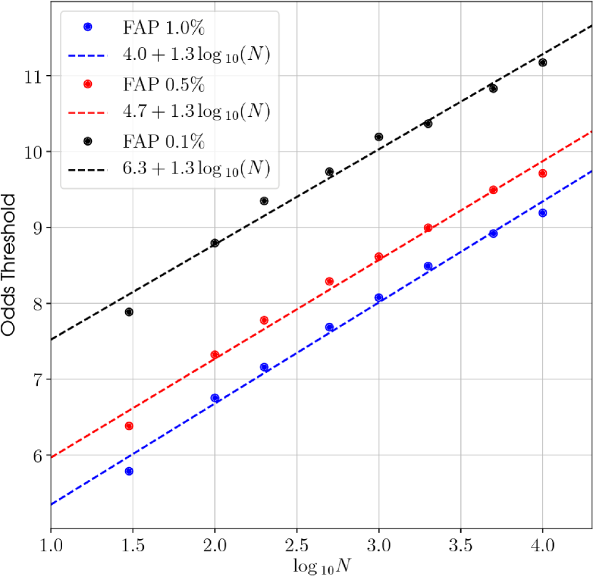
for which values above zero favour there being a change point in the data. We could simply use this as the criterion on which to split the data into two chunks at the change point value with the largest evidence. However, in practice this leads to data drawn from a single Gaussian distribution actually being split far too often, and also there being a dependence on the data length. So, instead, we empirically calculate an odds threshold above which the value of Equation 26 must be to impose a split in the data.444A different, but equivalent, approach would be to apply different priors to each hypothesis, although we have just taken the empirical approach. The empirical threshold we use is worked out by finding the 99% upper limit on the value of Equation 26 when data is purely drawn from a single Gaussian distribution (i.e. it gives a 1% false alarm probability) as a function of the data length . The results of doing this for 30 000 instances of data for a range of values, and three different false alarm probabilities (1%, 0.5% and 0.1%), are shown in Figure 6. Fitting a line to the 1% false alarm probability points gives an odds ratio threshold dependence of
| (27) |
The above process just splits the data once, so it must be applied iteratively to split the data further. When a change point is found then the process is repeated on the two split data chunks, and stops when either no change point is found within a chunk, or the split would give a segment smaller than .
2.5. Signal-to-noise ratio calculation
Whether a signal is found or not, the code will generate a signal-to-noise ratio (SNR). The calculated SNR uses the set of signal parameters, , that give the maximum value for the likelihood, which are then used to create the best-fit complex signal template . We then use calculations of the noise standard deviation for each data chunk after removal of a running median from the data (the splitting and running median are described in §2.4). The coherent SNR is then calculated as
| (28) |
using the notation given in §2.2.555If using data input from the spectral interpolation code (Davies et al., 2017) the noise standard deviations are actually passed to the code (see §A.1), so in Equation 28 is replaced by and is replace by as in §2.2.2.
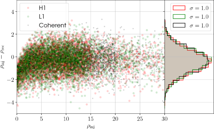
A plot of the residual between the recovered single-detector and joint detector SNRs and their true values666The true values are calculated by using the actual simulated signal model in equation 28, rather than the recovered maximum likelihood model. versus the true signal SNRs, as calculated from Equation 28, for a set of simulated signals (described in §4.1.2) are shown in Figure 7. The standard deviation of the residuals is found to be one, with a mean around zero, and the distribution does not appear to change as a function of SNR (except at the lowest SNRs, where the noise in the data will generally give rise to a maximum likelihood model with a larger amplitude than the true signal, and thus an overestimate of the recovered SNR).
2.6. Odds values
This is not explicitly a core function of the code, but here we will define some model selections (odds between competing models)
| (29) |
that can be produced from the output of the code. The code outputs two (natural logarithm) evidence values: the evidence for a coherent signal () in all the datastreams (multi-detector and multi-frequency-band), and the evidence () for the data consisting of Gaussian noise (in sets of stationary segments as described in §2.4). These can be combined in various ways for different model selection situations, and we will define three such situations here (see, e.g., Abbott et al., 2017, for two of these):
-
1.
the odds for a (multi-detector and multi-frequency-band) coherent signal versus (non-stationary) Gaussian noise, ;
-
2.
the odds for a (multi-detector and multi-frequency-band) coherent signal versus incoherent (between detector) signals, ;
-
3.
the odds for a (multi-detector and multi-frequency-band) coherent signal versus combinations of incoherent (between detector) signals or noise, (cf. Equation A6 in Abbott et al., 2017).
The first of these (actually also given in Equation 1.1) just requires the two evidence values, and
| (30) |
The second requires that the code has been run for a multi-detector analysis, and also individually for each detector, , to give and , and is given by
| (31) |
Such an odds is useful in vetoing strong incoherent signals that are therefore not astrophysical, e.g. instrumental lines (see, e.g., the similar line-robust statistic defined in Keitel et al., 2014). In both these cases it is assumed that the prior odds () between the two models are set to be equal and therefore are not explicitly given.
The third odds makes use of a compound model in the denominator with all evidences for all permutations of Gaussian noise or incoherent signal being used. If we have the set of single detector signal and Gaussian noise models , then (see, e.g., Equation 50 of Isi et al., 2017)
| (32) |
where is the prior on the coherent signal model, and are the priors for the signal/noise hypotheses for each individual detector. As there are two possible models for data in each detector, signal or noise, the number of logical or combined sub-hypotheses (see, e.g., the four sub-hypotheses used in Equation A6 of Abbott et al., 2017, where the priors in the denominator are the combinations that would be given from expanding out equation 32) in the compound model is just given by . In Abbott et al. (2017), and later in this document, we have assigned the equal probabilities to the coherent signal prior and to each of the sub-hypothesis priors in the denominator, so that they cancel out. However, other priors could be used.
It is also worth noting that in all the above cases the models (and sub-hypotheses) are mutually exclusive. This may not at first seem obvious, as, for example, the Gaussian noise model is contained within the signal model provided the prior on the signal amplitude allowed a value of zero. But, as noted in Li et al. (2012); Isi et al. (2017), within the signal noise hypothesis having an amplitude of exactly zero (as in the Gaussian noise hypothesis) occupies an infinitesimally thin slice of the parameter space, and therefore has no weight. The same can be said for the situation of a coherent signal model within the incoherent signal model.
3. Nested sampling setup
Here we will briefly describe some of the core functions used for the Nested Sampling algorithm (Skilling, 2006) within our code. We will not describe nested sampling itself, over-and-above the very brief summary given in §1.1, but instead refer the reader to Veitch and Vecchio (2010). We also refer the reader to Veitch et al. (2015) for a more thorough description of some of the concepts we will discuss below.
One main point about the nested sampling algorithm is that it starts by randomly drawing a certain number of samples (the number of which we call the number of live points, , which will be the constant number of “active”, or “live”, samples), where a sample is a vector, , containing a value for each parameter drawn from their respective prior distributions (see §2.3). The samples must be independent draws. For each of these samples the likelihood will be calculated and the sample corresponding to the minimum likelihood, , will be noted. As the algorithm progresses the number of live points stays the same, but at each iteration a new sample will be added in place of the one with the minimum likelihood, and therefore the minimum likelihood will continuously be updated to be the minimum value for the current set of points.
3.1. Proposal functions
The nested sampling algorithm requires a way to draw new samples from the parameter space that is being explored. The particular requirement for nested sampling is that any new sample is an independent draw from a constrained version of prior probabilty function for each parameter. The constraint is that the new sample’s likelihood must be greater than the current value of , e.g. for a single parameter , the probability of drawing a point at would be
| (33) |
where is the prior on .
There are various methods to sample from the constrained prior, the simplest of which is just to sample from the full prior and only accept a sample if it meets the likelihood constraint. However, such a simple method soon becomes very inefficient if the likelihood gets more and more tightly concentrated within the prior volume (which can happen rapidly for high-dimensional problems). One popular nested sampling method is MultiNest (Feroz et al., 2009), which performs the sampling by calculating a set of ellipsoids bounding the live points and drawing points uniformly from within them. Various other approaches exist such as Diffusive Nested Sampling (Brewer et al., 2011; Brewer and Foreman-Mackey, 2016) and POLYCHORD (Handley et al., 2015).
The version of nested sampling used in the LALInference library, as used by our code, makes use of a Markov chain Monte Carlo (MCMC) approach to drawing new samples (Veitch and Vecchio, 2010). The MCMC attempts to sample from the constrained prior distributions in an efficient manner, with the final sample of the chain being a statistically independent sample from the rest of the live points. To sample most efficiently the MCMC requires a proposal distribution that closely resembles the underlying constrained prior that it is trying to sample from. LALInference has a variety of potential proposal distributions (Veitch et al., 2015), but our code currently allows five different proposals, that can be used in different proportions:
- Ensemble walk
-
This is one of the affine invariant ensemble proposals described by Goodman and Weare (2010), which adopt the scale and shape of the current set of samples. The hard-coded setup in LALInference is that three samples randomly drawn from a cache of samples are used to define the “walker” samples. This is the main default proposal of our code, and is used as the proposal 75% of the time.
- Ensemble stretch
-
This is another affine invariant ensemble proposal described by Goodman and Weare (2010), and makes use of two samples randomly drawn from the sample cache. By default this proposal is not used at all.
- Differential evolution
-
This is similar to the stretch proposal in that it uses two samples randomly drawn from the sample cache. By default this proposal is not used at all.
- Uniform proposal
-
This proposal just draws points from their full prior for parameters that have a uniform prior specified. Other parameters are not evolved. This proposal is used 25% of the time by default.
- Frequency jump
-
This proposal tries jumping between Fourier frequency bins if frequency is one of the required parameters. This proposal has not been tested and, by default, is not used at all.
The cache of samples mentioned above, and used by the nested sampling algorithm, is the set of live points, but this cache is only updated on iterations of the algorithm that are a factor of 10% of the number of live points (e.g., for 1000 live points the cache is updated after every 100 new iterations).
The length of each MCMC run can be chosen by the user, but by default it is automatically set within the code. To do this, at the same rate as the cache is updated, the autocorrelation length of the parameters is calculated. A random sample from the current live points in chosen, and evolved via the MCMC, and the autocorrelation length of each parameter, , is calculated. The number of MCMC iterations, , is then chosen as , where 5000 is a hardcoded maximum length.
3.1.1 Testing the proposals
We would like to test whether some of the above proposals lead to accurate calculations of the evidence integral as given in Equation 1. It is especially interesting to do this for a variety of prior volumes, starting of with volumes similar to the posterior volume, but then diverging to be much larger than the posterior volume (or in other words, as the information gain, , or Kullback-Leibler divergence, increases). To do this our code has the option of setting a one-dimensional Gaussian distribution as the likelihood function, using a flat prior bounded between and , and working out the evidence. Analytically the evidence is given by
| (34) |
As we are often interested in setting upper limits of, for example, the gravitational wave amplitude , we can also use the test to see if the upper limits we obtain from the posterior samples match the expected upper limit obtained (via root finding) from the CDF of the distribution
| (35) |
where is the area under the distribution. We can calculate the true Kullback-Leibler divergence via {widetext}
| (36) |
where is the posterior, the likelihood, and is the prior (with ), and is the evidence calculated via Equation 3.1.1. For the case of and , and provided , this generally simplifies to
| (37) |
A final thing that we can check, on top of the upper limit value, is whether the posterior samples appear to be drawn from the expected posterior distribution. To do this we use a Kolmogorov-Smirnov test comparing the CDF of the samples with the analytical CDF and calculating the two-sided -value for the null hypothesis that the two distributions are the same.
In the tests below we have run the code on this Gaussian likelihood with a Gaussian of zero mean and , truncated at zero by fixing the lower prior bound to . This is similar to the form of the likelihood seen in pulsar searches when no signal is present. We have then set a range of upper bounds, , from to increasing by a factor of ten each time, and a range of numbers of live points from to increasing by powers of two each time. For each combination of upper bound and number of live points we have run the code on the test Gaussian likelihood 100 times to see the statistical spread of the output.
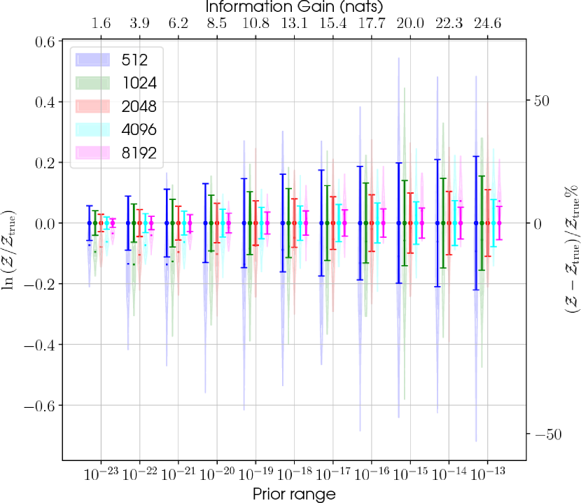
In the first test we check how using only the ensemble walk proposal (which is not the default configuration described above) fairs at estimating the evidence, upper limit, and posterior distribution. Figure 8 shows a variety of information, but it primarily shows the distribution of the ratio of evidences output from our code, , to the true evidence calculated via Equation 3.1.1 as a function of the value of the upper prior bound (or equivalently on the top axis the information gain, in natural units of information (nats), calculated via Equation 3.1.1). This is shown for the range of different numbers of live points used. It is clear that as the information gain increases (i.e. the posterior is constrained within a successively smaller part of the prior range) we are systematically more biased towards overestimating the evidence. It can also be seen that the bias increases with increasing number of live points. Linear fits (in and , the information gain) for different numbers of live points are shown in Table 1. It is interesting to note that the statistical spread of values (if ignoring the systematic offset) are consistent with the expected range given by the error bars, and calculated using (Skilling, 2006), where here is the mean of the information gain (in nats) returned by the nested sampling algorithm for each run.
| 512 | 0.045 | |
| 1024 | 0.058 | |
| 2048 | 0.065 | |
| 4096 | 0.068 | |
| 8192 | 0.070 |
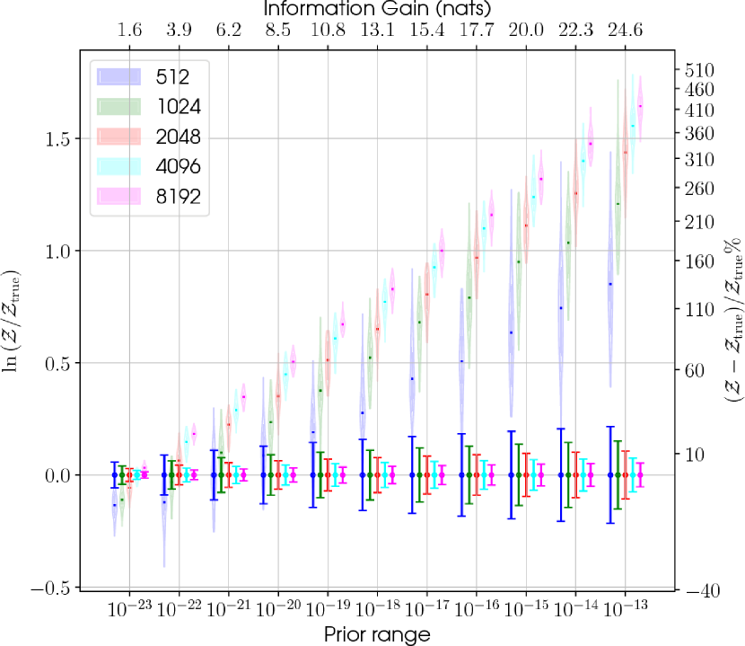
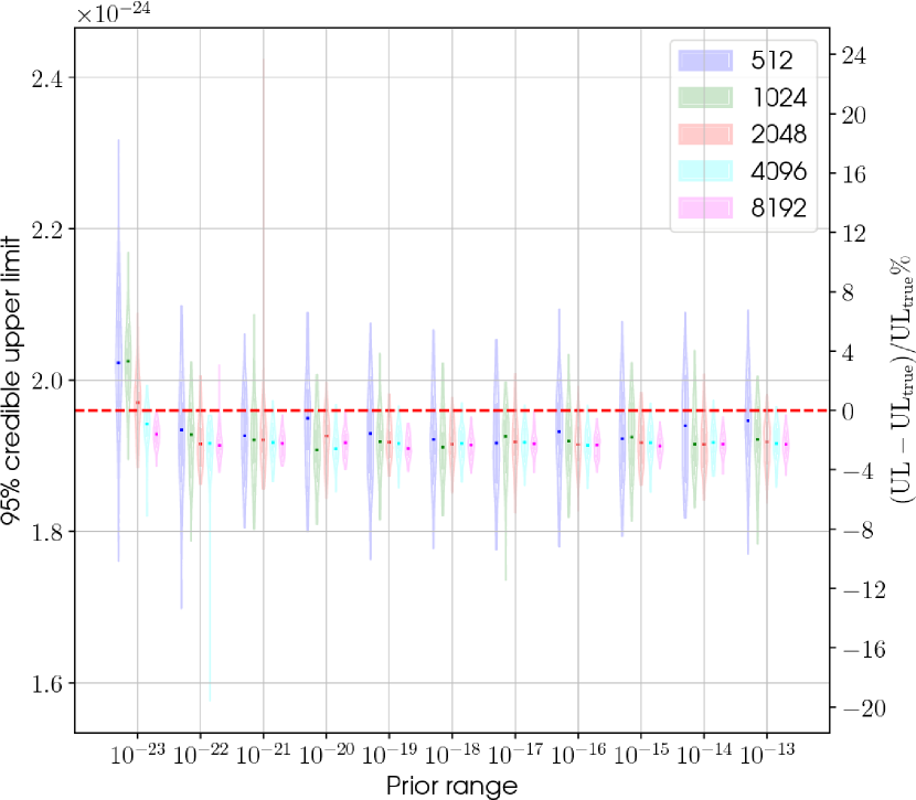
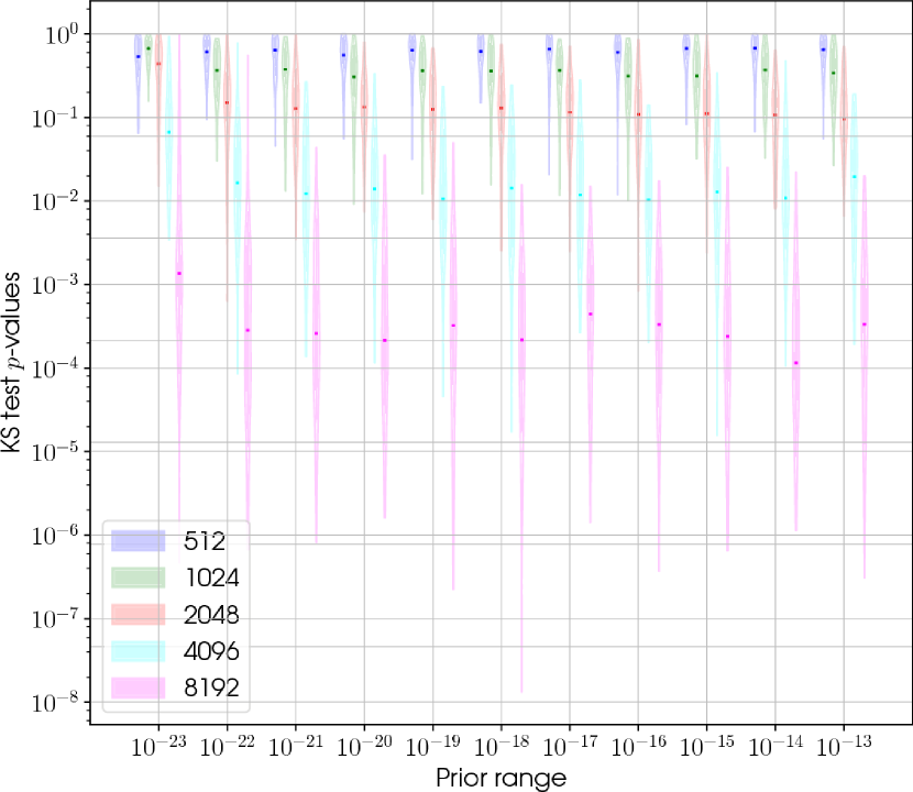
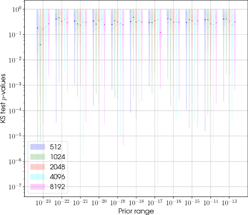
Figure 9 shows the distribution of 95% upper limits on the parameter in Equation 35 (calculated by solving the equation for ). It can be seen that, other than for the narrowest prior range, there is a systematic bias towards the upper limit being underestimated by . Figure 10 show the distribution of two-sided -values from a Kolmogorov-Smirnov test comparing the CDF of posterior samples against the analytical CDF in Equation 35. The -value null hypothesis is that both distributions are the same, and it should be noted that we performed 100 trials for each prior range value and number of live points. For the lower numbers of live points the distributions appear to be consistent, however, for larger numbers of live points the distributions are rather inconsistent a large amount of the time. This is most likely due to differences in distributions showing up more obviously when there are more posterior samples to use.
The systematic biases in evidence values and upper limits may not be a major problem777The evidence biases at the level seen are unlikely to sway model comparisons as they will most likely show up when one model is very highly favoured over another. The observed biases in the upper limits are at a level that is currently less than expected uncertainties due to instrumental calibration., but does point towards there being some issue with the implementation of the ensemble walk proposal.
In the second test we have checked what happens with the code’s current default proposal settings: using the ensemble walk proposal 75% of the time and the uniform proposal 25% of the time. It should be noted that this default is not arbitrary, but came about from tests similar to these when just using the ensemble walk proposal.
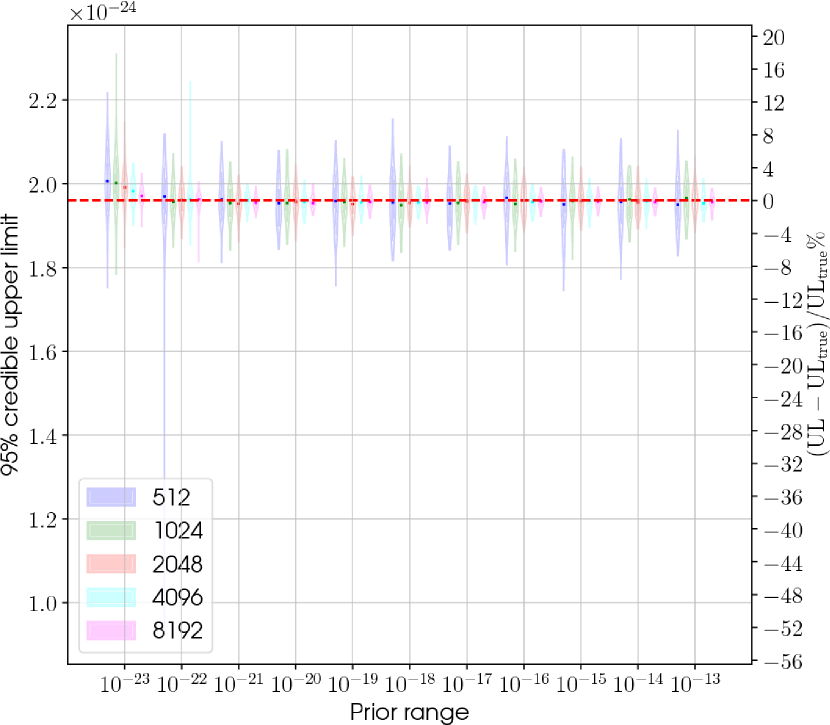
Figure 11 shows the evidence distributions equivalent to those in Figure 8. However, what can be seen in this case is that there is no obvious systematic bias as a function of , and the statistical uncertainty is consistent with expectations (as shown by the error bars). Similarly, the upper limits and Kolmogorov-Smirnov -values shown in Figures 12 and 13 respectively are consistent. The reason why this combination of proposals seems to work whereas the ensemble walk proposal on its own does not is currently not understood, but we plan more work on figuring this out.
3.2. Posterior sample generation
As discussed in §1.1 nested sampling codes, such as lppen, do not intrinsically output samples that can be histogrammed to give representations of marginalised posterior distributions for the model parameters. They instead output an ascending likelihood ordered list of samples, each of which occupies a known approximate amount prior volume. Samples must be drawn from these, with appropriate weighting (see Equation 4), to give a new set of samples that does represent the posterior distribution. During this process it is also possible to appropriately combine samples from parallel independent nested sampling runs (weighting each based on their calculated evidences) to recalculate the evidence and generate posterior samples.
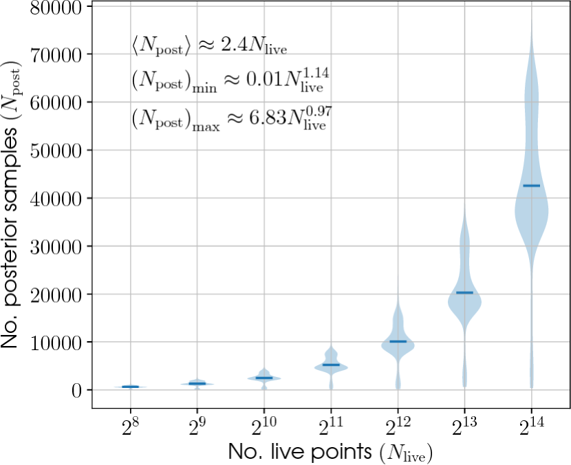
What is described above is not a core function of the lppen code, but is an integral part to generating results with it, and has been used to produce the posterior distributions discussed earlier in the section, and later in this document. The number of posterior samples generated by the code is dependent on the number of live points used when running nested sampling. The actual dependence of the number of posterior samples on can be seen in Figure 14 (this uses the simulations discussed in §4.1.3). It can be seen empirically, that the mean number of posterior samples goes roughly as , although there is a lower tail extending to .
3.3. Code timing
How long the code takes to runs depends on two main factors: the number of live points used and the information gain going from prior to posterior. Increases in both of these will generally mean that the code takes longer to run. Using the simulations from §3.1.1 we have assessed the code run time for the simple testing Gaussian likelihood function. This allows us to quantify the code run time as a function of both number of live points and information gain.
We find that the median calculation time for the simple Gaussian likelihood function used in §3.1.1 (on an Intel “Haswell” processor, specifically Intel CPU E5-2680 v3 @ 2.50GHz), including some standard overheads888Without the overheads it is roughly seconds. is seconds. The median time for calculation of the likelihood (including model calculation time) for a standard search (Eqn. 2.2.1) over only non-phase evolution parameters, and for one chunk of data, is seconds.999Without the additional overheads this is a similar time of seconds.
The median run time per likelihood evaluation for the nested sampling part of the code for the standard likelihood function (using 1024 live points) is seconds, which is times greater than the single likelihood evaluation time (this ratio will change as a function of the number of live points). The median run time per likelihood evaluation for the nested sampling part of the code for the test Gaussian likelihood function (using 1024 live points) is seconds, which is times greater than the single likelihood evaluation time.
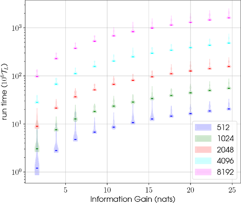
In Figure 15 we show the time taken for the runs in §3.1.1, using the default proposals, as a function of number of live points and information gain. The code run time is divided by to provide a way to scale it for other values of , e.g. that found from the code’s standard likelihood function. If we perform a 2D linear fit to the natural logarithm of the median run time, , we get the relation
| (38) | ||||
| (39) |
This relation should be considered as a rough lower limit to the run time for any particular likelihood function. Above, we saw that for our standard likelihood function the nested sampling algorithm was roughly three times quicker per likelihood evaluation than the simple test function. In both cases the internal MCMC, which draws new samples within the algorithm, required very similar small lengths to give uncorrelated samples, so there must be other internal bottlenecks that make the simpler likelihood relatively slower. However, in general, longer MCMC chains will be required to give uncorrelated samples, so the number of likelihood evaluations will increase.
4. Evaluating the code
Here we will evaluate the code in a variety of ways. We compare a selection of posterior probability distributions generated using lppen, over a range of signal parameters, with those produced using a previous code. We also use a selection of many simulated signals to show how the odds comparing a signal model and a noise only model change with signal-to-noise ratio, along with comparing coherent verses incoherent signals (for coherent simulated signal and incoherent simulations). The simulations also allow us to evaluate the posterior probability distributions produced by the code using what is colloquially known as “P-P plots” (see §4.3.1)
4.1. Code comparison
In this section we will show how the posterior parameter distributions that we can generate from the output of our nested sampling code compare to evaluating them with a previous implementation of the analysis code (lalapps_pulsar_parameter_estimation, or for the rest of this document shortened to lppe, used in, e.g., Aasi et al., 2014) using a (generally inefficient) MCMC algorithm and over a grid in parameters.101010For the MCMC examples in this section, we have used “burn-in” periods of 100 000 iterations, followed by 500 000 posterior sample iterations, from which there have been roughly 1000 independent samples used to produce the posterior plots. For the grid-based examples the grid sampling used has been . We will show comparisons of the codes in two different regimes: no signal is present in the data, and an obvious signal is present in the data. We do this using simulated data both containing purely Gaussian noise and containing simulated signals added to Gaussian noise.
In each of the tests below we will be running our code (lppen) using the default proposal distributions discussed in §3.1 and with the number of live points fixed to be 2048. We will also assume a source at a fixed sky position and that the signal model is purely that for the harmonic (Equation 8), and that we work in terms of the signal amplitude and signal phase (this is for consistency with the old code which uses rather than , which we have earlier defined as the rotational phase). The simulated data in all cases will be generated as the complex heterodyned time series sampled once per minute. When comparisons between the current code and previous codes are made we run the current code in a way that splits datasets into 30 point chunks, rather than using the algorithm described in §2.4, as this makes it consistent with the old code (lppe). We also purely use the uniform prior ranges for the amplitude parameter to be consistent between codes.
4.1.1 Simulated noise
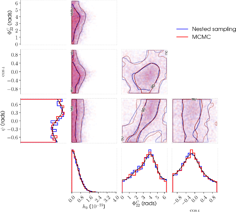
An initial test of the code is whether the output posterior probability distributions match those produced when evaluating the posterior over a fixed grid in the four-dimensional parameter space of , when using purely Gaussian noise.111111It is worth noting that in many of these tests the polarisation angle prior covers to rather than the 0 to range given in, e.g., Pitkin et al. (2015), due to this being the range required by the older parameter estimation MCMC code. Although this range is degenerate to rotations over , so spans the same range of waveform models. A comparison of the marginalised posteriors for individual parameters, and pairs of parameters, are shown when using simulated data lasting ten days from a single detector (in this case assumed to be the LIGO Hanford detector, H1) in Figure 16.
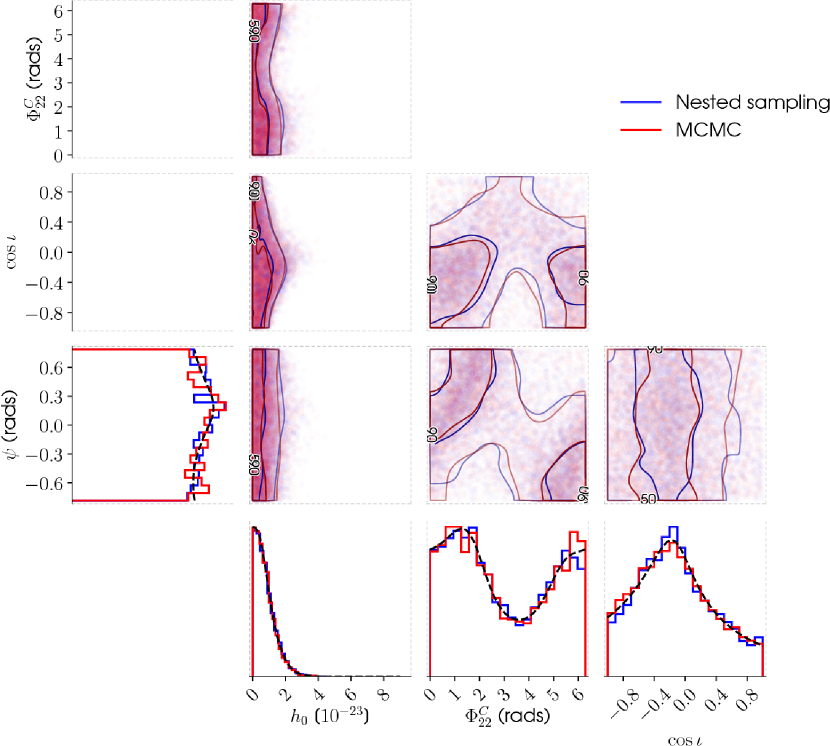
It can be seen that the output posteriors look qualitatively consistent. However, we can also quantify some aspects of consistency by comparing the evidence output from the nested sampling code with that estimated from the grid-based method from lppe, the upper limits on produced by the codes, and performing Kolmogorov-Smirnov consistency tests between the nested sampling posterior samples and MCMC posterior samples (giving a -value for the null hypothesis that the samples are from the same distributions). These are shown in Table 2 and show very good consistency between the codes, although it should be noted that these are for one particular run and some statistical fluctuations in the exact values for different runs are to be expected (see, e.g., the variations in evidence values in §3.1.1). A jupyter notebook with this test can be found here.
| Simulation | K-S -value | |||||
|---|---|---|---|---|---|---|
| Noise (single detector) | 0.404 | 0.026 | 0.010 | 0.703 | ||
| Noise (two detectors) | 0.141 | 0.564 | 0.538 | 0.493 | ||
| Signal (single detector) | 0.245 | 0.237 | 0.291 | 0.125 | 0.175 | |
| Signal (two detectors) | 0.240 | 0.991 | 0.722 | 0.052 | 0.067 | 0.032 |
We see a very similar situation, in terms of agreement between the codes, when running on simulated data assumed to be from two detectors (the LIGO H1 and L1 sites) as shown in Figure 17 and the second line of Table 2. A jupyter notebook with this test can be found here.
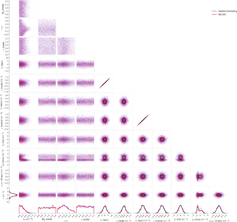
The above tests using simulated noise, and with searches covering the four standard unknown gravitational wave parameters, show that the code appears to be working as expected, and is in agreement with our previously used code. However, more generally we can perform parameter estimation over a larger number of signal parameters, and can again check for consistency with the previous code. We produce one day of Gaussian noise for a single detector and search over the four gravitational wave parameter with the same priors as before, but then also use a multi-variate Gaussian prior (§2.3.2) over the phase parameters: rotational frequency and first frequency derivative, and binary parameters of binary period, time of periastron, angle of periastron and its first derivative, projected semi-major axis, and eccentricity (). This gives a total of 12 parameters in the search. The multi-variate prior is defined such that all parameters are uncorrelated except, in this case, the parameter pairs and for which we use a very high correlation of (we do not set them to be fully correlated due to numerical issues inverting such matrices).
The one-and-two dimensional posteriors (expressed as offsets from the assumed heterodyne parameter values) output for this case when run with both lppe and lppen can be seen in Figure 18, which also overlays the marginalised priors on top. It can be seen qualitatively that the codes are consistent121212It is worth mentioning that in performing these tests a bug was discovered in lppe in which Equation 10 was being applied with the wrong sign, leading to parameter estimates having the wrong sign. However, this bug was fixed for the example shown here. and for the phase parameters the priors are recovered, except for , which has some structure due to the specifics of the noise realisation. The Kolmogorov-Smirnov test -values testing the null hypothesis that the posterior samples from each code are drawn from the same distribution are shown in Table 3, and suggest that the distributions are consistent.
| Parameter | ||||||||||||
|---|---|---|---|---|---|---|---|---|---|---|---|---|
| -value | 0.13 | 0.04 | 0.78 | 0.23 | 0.44 | 0.26 | 0.85 | 0.28 | 0.29 | 0.86 | 0.52 | 0.28 |
4.1.2 Simulated signals
The next test is checking how the codes compare when there is a signal present in the data. When generating the simulated signals131313Simulated signals used in this work have either been generated directly using lppen (see, e.g., Appendix A.1.4), or using functions within the pulsarpputils.py python module in lalapps within LALSuite (LIGO Scientific Collaboration, 2017). we initially assume that the signal’s phase evolution is perfectly known and has been removed via the heterodyne described in §2.1, and therefore from Equation 10. As in §4.1.1 we search over the four-dimensional parameter space of .
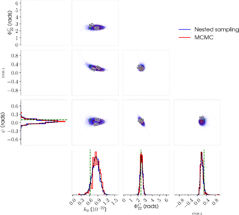
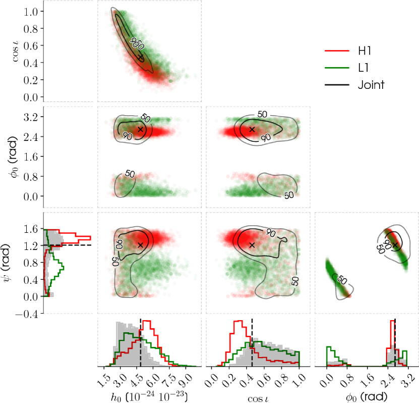
We create a simulated signal in the H1 detector spanning ten days of data with parameters (, rad, and rad) that produce a signal-to-noise ratio of 8 when injected into Gaussian noise. The posterior probability distributions estimated for the parameters (expressed as offsets from the assumed heterodyne parameter values) are shown in Figure 19, which show consistency between the old and new codes and with the injected signal parameters. The quantitative consistency between the codes can be seen in Table 2, where is should be noted that the evidence ratio between the codes is larger than statistical uncertainty would expect, although the fractional difference between the values () is still small enough to not greatly effect conclusions drawn from either values if used in model selection.
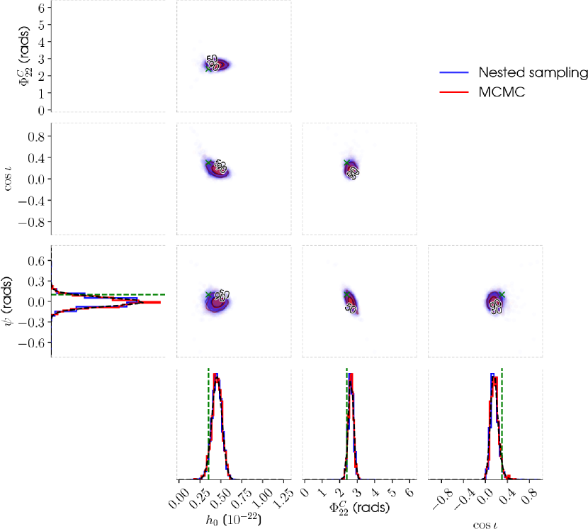
Similarly, using a signal with a coherent multi-detector signal-to-noise ratio of 8 (for the same parameters as above except with ) when simulated and injected into Gaussian noise for two detectors (H1 and L1) we see the posteriors shown in Figure 20, and consistency checks in Table 2. The notebooks for the above two tests can be found here and here.
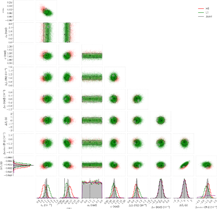
A set of simulated signals with sky location and orbital parameters set to those of the Low-mass X-ray binary Sco X-1 were injected into Gaussian noise for the study in Messenger et al. (2015). As a test of our code when recovering a signal from a source in a binary system we have recovered one of these signals using approximately 1.4 days of simulated data. We have purposely performed the heterodyne data processing stage with values of several of the phase parameters (, , , and ) set to not match the known simulated signal values. Therefore, to recover the signal, in addition to the four gravitational wave parameters we have had to allow the code to search over these extra parameters. For these additional parameters Gaussian priors were used, with the prior means set to be the parameter values used for heterodyning (not those for the actual signal), with standard deviations wide enough to encompass the true signal values. For a Fermi-Dirac prior was used, whilst flat prior were used for the other angle parameters, covering their minimal allowed ranges. The recovered signal posterior distributions can be seen in Figure 21, which show that the true parameters are correctly recovered (the plot shows recovered phase parameters as offsets from the heterodyne parameter values, i.e. the centres of the Gaussian priors). It can be seen that for and the posteriors contain the correct value, but are peaked well away from the value used for heterodyning (which would be at zero in the plots), showing the code’s ability to explore the prior space in these parameters. The one-dimensional marginal distribution for spans the full prior range, however, this is due to it being highly correlated with , and, although not visible on the plot, this very strong correlation is present in the two-dimensional posterior for these parameters. Finally, for and , it can be seen that the posteriors just fill the prior ranges as the data provides no additional information about these parameters. For completeness, we find that the signal was recovered with SNRs of in both H1 and L1 individually, with a coherent SNR of , and odds values for the multi-detector analysis of and .
4.1.3 Results evaluation
The above results have shown good qualitative, and quantitative, agreement between the old and new codes for individual cases, but it is also useful to see how they compare for a large number of noise realisations when assessing two important quantities: the 95% upper limit on gravitational wave amplitude , and the signal model evidence. It is also useful to see how these compare as a function of the number of live points used by the code. To this end we have chosen numbers of live points from 256 to 16384, increasing in a power of two for each step, and for each number generated 500 realisations of complex Gaussian noise with 1440 points over one day. Choosing a random source sky location for each realisation, and using uniform priors for the parameters , , and , we have performed parameter estimation using both lppen and lppe in its grid-based mode. For lppe the integrals required for calculating the signal evidence and 95% upper limit on are performed using the trapezium rule, whilst for the output of lppen the upper limit has been calculated using a greedy-binning approach bounded from zero. This assessment is very similar to what we did in §3.1.1, but has not just used a fixed Gaussian likelihood function in each case. We will make the assumption that the grid-based results are a representation of the true values for the evidence and upper limit, however, it should be noted that there will in fact be errors (and potentially biases) from the trapezium rule approximation.
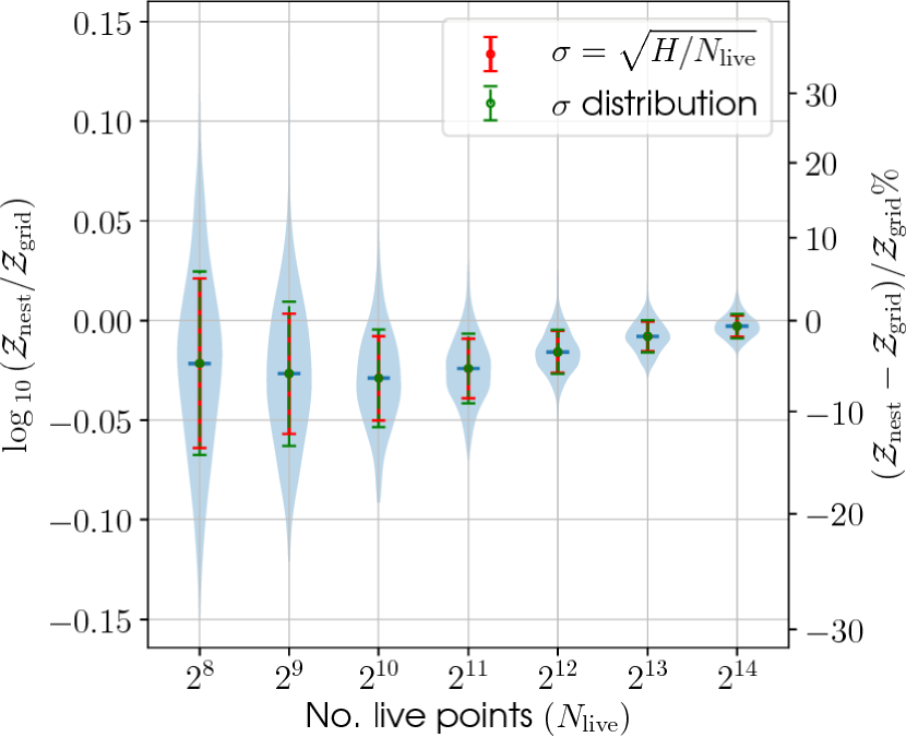
In Figure 22 we see a comparison between the signal evidences evaluated using nested sampling and the trapezium rule. The left-hand axis shows the logarithm of the ratio of the two values, whilst the right hand axis shows the actual percentage difference between the evidences. These are plotted as a function of the number of live points used in the nested sampling evaluation by lppen. We find that the distribution of evidences very closely follows the theoretically expected distribution calculated as (see §3.1.1), where given our prior range set up we found . It can also be seen that there is a slight bias towards the nested sampling evidence being underestimated by a few percent, as was also observed for the simple Gaussian likelihood function case in Figure 11.
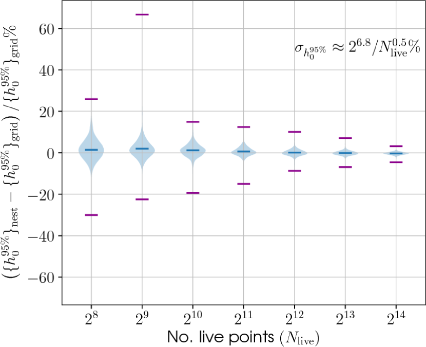
In Figure 23 we see a comparison between the 95% upper limits on as a function of the number of live points. The core distribution of upper limits produced via nested sampling are centred around the true (or grid-based) values, with the distribution decreasing in width with increasing numbers of live points. The standard deviation on the distribution roughly follows . The figure shows some extreme outliers in the distributions, but it is found that these outliers occur in the cases when the number of posterior samples drawn from the nested samples is extremely low (the lower tails of the distributions in Figure 14).
4.2. Injections into real data
During all bar the first initial LIGO science run, simulated signals from a variety of sources have been physically “injected” into the detector datastreams. These are known as “hardware injections” (see Biwer et al., 2016, for a general discussion of hardware injections, in particular relating to their use, and extraction, in advanced LIGO’s first observing run). These have included a range of continuous wave signals of the form given by, e.g., Equation 2 of Abbott et al. (2017), which in past have been searched for using a variety of analysis pipelines, including the one described in this document using lppe (see, e.g., Appendix B of Abbott et al., 2007).
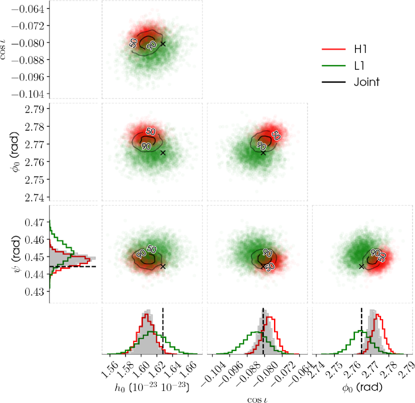
Here we have used lppen to perform parameter estimation on the parameters for two hardware injections added to intial LIGO data from the sixth science run (S6).141414 is being used here as opposed to as we are not having to compare to the previous code.151515S6 data is publically available at https://losc.ligo.org (Vallisneri et al., 2015). These are two out of the thirteen total continuous wave injections and were called “Pulsar03” and “Pulsar05” respectively. The data have been heterodyned with the known phase evolution of the signals. The extracted posterior distributions can be seen in Figures 24 and 25 and are in very good agreement with the injection parameters.161616For these hardware injections exact agreement between the expected injection parameters and those recovered, or between detectors, is not entirely expected. This is due to the injections needing to be performed using actuation functions (converting the expected gravitational wave strain into a force required to be exerted in the interferometer test mass) that may not exactly match the actuations functions later required for calibrating the detectors. For “Pulsar03” the signal is recovered with SNRs of 164 and 96 in H1 and L1 respectively, and a coherent SNR of 190, and with and . For “Pulsar05” the signal is recovered with SNRs of 9.9 and 6.4 in H1 and L1 respectively, and a coherent SNR of 11.8, and with and . The odds would imply a very high significance in distinguishing the coherent signal model from the noise models.
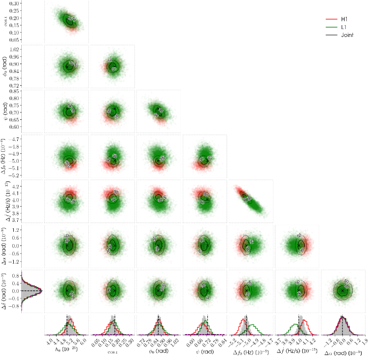
Several thousand simulated signals have been added to the LIGO sixth science run dataset (see Section IV of Walsh et al., 2016). For one particular signal (chosen for its moderate SNR over the run) we have used lppen to perform parameter estimation on the parameters . In this case, as for the binary signal discussed in §4.1.2, we have purposely heterodyned the signal using values of and offset from their known rotational values by Hz and Hz s-1.171717The frequency offset is approximately two Fourier frequency bins away from the actual signal frequency. We have used the whole of the S6 dataset, spanning almost 1.3 yr, with roughly 50% duty factors for both H1 and L1. The code was run using the ROQ mode for each individual detector and a joint detector analysis. Gaussian priors were used on the frequency and sky location parameters. The recovered marginalised posterior distributions can be seen in Figure 26, where all parameters are observed to be correctly recovered at their true values, even and which we offset (it is hard to see in the plots, but these values are constrained well within their allowed prior ranges). This signal was recovered with SNR of roughly 29 and 21 in H1 and L1 individually, and with a coherent SNR of 35. The odds values are and showing that the signal is very significantly distinguished from the noise model.
4.3. Monte-Carlo studies
In this section we will assess the outputs of lppen using a range of simulated signals. We have created two sets of 2000 signal parameters with which to inject simulated signals into Gaussian noise (with the same standard deviation of ) for the H1 and L1 detectors. Both sets have been generated with , and drawn from uniform distributions over their minimal allowed ranges (Table 1 of Pitkin et al., 2015), but for the first set is calculated such that the coherent SNR (Equation 28) is drawn uniformly between 0 and 20; the second set draws the uniformly between 0 and , such that the maximum coherent SNR (given the known noise level) is . This latter set is used to evaluate the posterior distributions as described below in §4.3.1, whilst both sets are used to evaluate odds distributions. The sources’ sky locations are drawn uniformly from over the sky-sphere. For these analyses each simulated data set is one solar day long, consisting of 1440 complex data points (generated as if heterodyned at precisely the known source phase evolution) sampled once per minute. This data has been used to estimate the four parameters , , and , with each being given a flat prior: the angles and cosine of orientation angle over their minimal ranges, and between zero and (well above the extent of the bulk of the likelihood). When running lppen on these, two parallel runs with 1024 live points where used, along with the default sampler proposals described in §3.1, and with the samples from both runs being combined to produce posterior samples and evidence estimates.
Another set of 2000 simulations has been created that again create simulated signals and add them to Gaussian noise for the H1 and L1 detectors. In this case the total SNR shared between the detectors has be drawn from a uniform distribution between 0 and 30, however, the signals have been purposely created to be incoherent between detectors to simulate instrumental noise features. The parameters , and are drawn from their minimal allowed ranges, but are different for the signals input into the two detectors, whilst the sky positions are also independent for both detectors. The signal rotational frequency and frequency derivative are also offset between detectors, such that the offsets are drawn from Gaussian distributions of () width Hz and Hz respectively. The length of the data is the same as in the previous case, but it is assumed that the data for both detectors was heterodyned using the known phase evolution for the signal in only the H1 detector. The same prior and run settings as above were used. These simulations have been used for assessing the odds for a coherent versus incoherent signal (see §2.6).
Finally, two sets of simulations of 500 signals have been created to assess the code when estimating additional phase parameters: in this case the rotational frequency , frequency derivative , and right ascension . Gaussian priors on these three parameters have been used, with parameters given in Table 4. These Gaussian priors are used when generating signals and when estimating them using lppen, whilst the simulated data is created such that it was heterodyned using the mean values. As above, one set of these simulations has amplitudes calculated such that the coherent SNRs are drawn uniformly between 0 and 20, whilst the other has amplitude drawn uniformly between 0 and . The latter of these is used to evaluate the posterior distributions, whilst both are used for odds distributions assessment. Again, the angles are drawn uniformly from their minimal ranges and sky positions are drawn uniformly over the sky-sphere.
| Parameter | mean | standard deviation |
|---|---|---|
| (Hz) | 100 | |
| (rads) | () |
4.3.1 Evaluating the posterior distributions
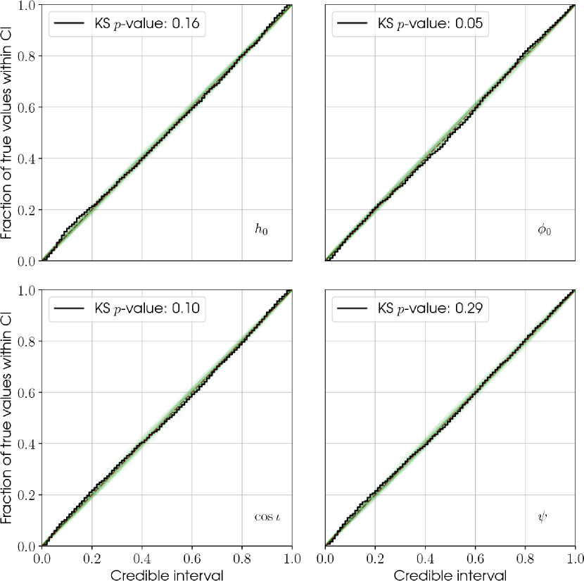
In Sidery et al. (2014) a method was developed for evaluating whether sky location credible intervals for compact binary coalescence gravitational wave signals, produced from posterior distribution output by LALInference codes (Veitch et al., 2015), behaved self-consistently. The approach uses injected signals, with parameters drawn from the prior distributions used when reconstructing them181818In this case the amplitudes of the simulations are not drawn from the full prior range, but are drawn from a flat distribution within that range, so are valid for this comparison., and sees if the credible intervals effectively behave as frequentist confidence intervals, i.e. do 50% of the known parameter values fall within some pre-specified definition (like the minimal credible region, or credible region bounded by the lower extent of the prior) of the 50% credible region. This can test whether the underlying LALInference parameter sampling is working as expected, or if there are biases to wider, or narrower, credible regions. The method, and the “P-P plots” it produces through evaluation over a range of credible intervals, has now become commonly used to assess the LALInference parameter estimation codes (Veitch et al., 2015) as a way of highlighting any problems.
We have used this method here to evaluate our parameter posteriors produced from the simulations described above for which the amplitudes were drawn from a uniform distribution. For each simulation we have calculated the minimal credible region from the one-dimensional marginalised posterior samples that the injected value falls within (using a greedy-binning approach). The cumulative histogram of these values, for each parameter when using the simulations that just estimate the four gravitational wave parameters, can be seen in Figure 27. Also, shown for each parameter is a Kolmogorov-Smirnov test -value comparing our observed distribution to a uniform distribution, and a “cloud” of cumulative distributions that are random realisations of the expected cumulative distribution. We see that, overall, our posteriors give credible intervals that behave as expected, without any large deviations.
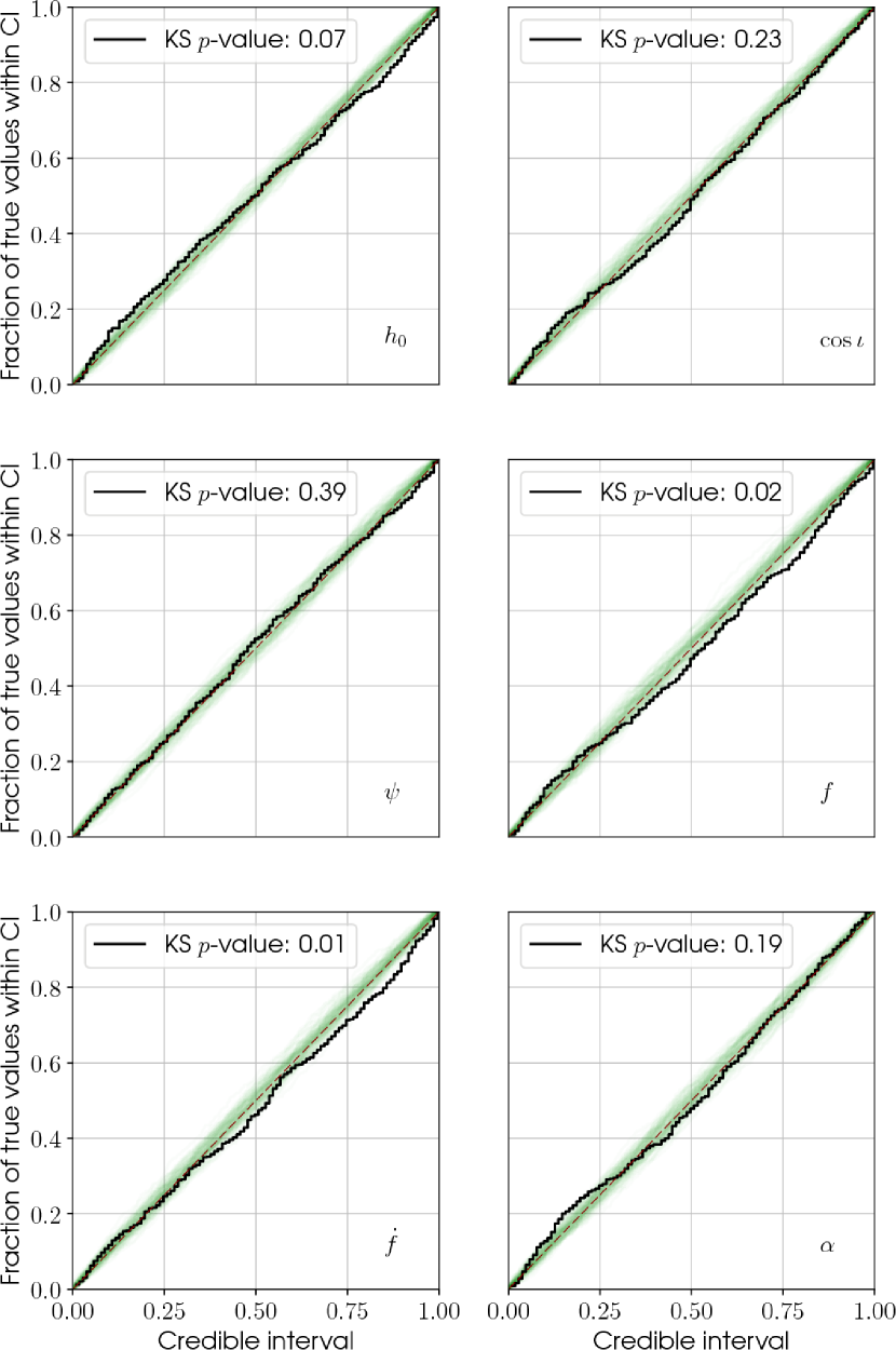
Similarly, we have done the same thing for the posteriors produced from the simulations that included searches over , , and . In this case we know that the parameters are and are completely correlated (i.e. there is a degeneracy), so we have held the value of fixed at zero.191919In cases where there is a complete degeneracy between parameters the samplers used in the code can have problems, leading to observable effects in the “P-P plots”. In certain cases, where the degeneracies are known, there are ways to deal with this: one parameter of a degenerate pair can be held fixed, a custom proposal distribution can be hard coded for degenerate parameters that deals with the correlations, or, reparameterisations can be found that do not have the degeneracies. In the future the latter of these may be implemented in our code to deal with strong degeneracies between the initial phase and derivatives of it (frequency, and further frequency derivatives). Such a parameterisation could involve using, e.g. the start and end phase, rather than and , with further derivatives being incorporated through additional phase parameters at fixed times throughout the model. So, as another example, rather than internally sampling in , , and , one could use , , and , and convert between the two using linear algebra. These “P-P plots” can be seen in Figure 28, where generally we see posterior credible intervals behaving as expected.
4.3.2 Evaluating the odds
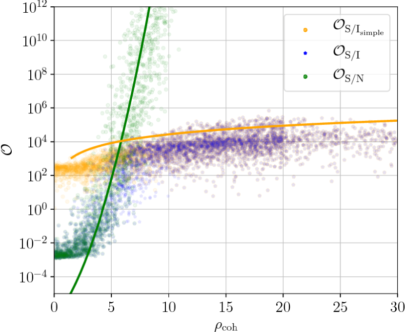
It is useful to see how the odds values, described in §2.6, look when calculated for our simulations. As mentioned above, along with coherent signals between two detectors, we have purposely created incoherent signals to see how the odds look. Firstly, just considering the coherent simulations, we can see in Figure 29 how the odds , and (Equations 2.6, 32 and 2.6, respectively) vary as a function of coherent SNR. We see that rapidly increases, has a shallow growth, whilst transitions between following at very low SNR to matching at higher SNR. This behaviour is consistent with our expectations described in Appendix D with and . We note that the locations of these distributions on the y-axis can be strongly effected by the prior volume, changes to which will move the distributions up or down, and can affect where they intersect. However, the general shape of the distributions should be very similar.
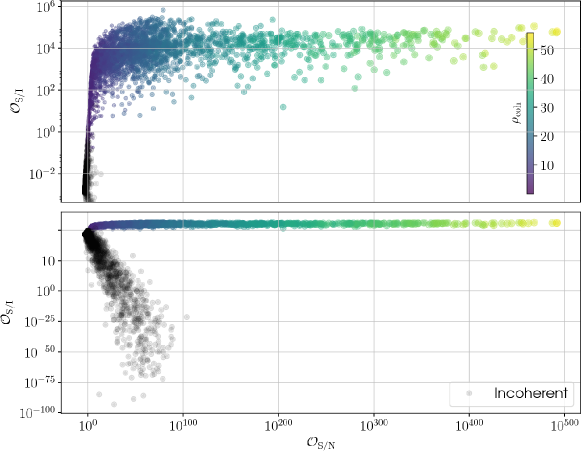
In Figure 30 there are two panels showing as a function of . In the upper panel (showing the coherent simulations) the colours of points show the signal’s coherent SNR. The plateauing of is just that seen in Figure 29. The bottom panel shows a zoomed out version, with the incoherent signals as dark circles (these are also seen in the lower left of the upper panel). Here we see that for incoherent signals the value of between the coherent and incoherent signals diverges quite quickly, with falling off roughly linearly with . This shows that, hopefully, for reasonable strength signals the value of will be useful for distinguishing a coherent from an incoherent (and therefore not astrophysical) signal.202020The caveats to this are that the way we created our incoherent signals may not well match true signals caused by instrumental (non-astrophysical) effects in gravitational wave detectors. However, we hope our simulations are extreme, in a conservative way, in that one detector is actually containing an unadulterated signal, and is therefore potentially producing a far larger value than might be expected whereas an instrumental feature would generally not match our signal template, even in a single detector.
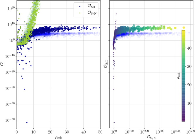
It is useful to see how these distributions change when the parameter space searched over increases in complexity. So, in Figure 31 we see similar plots to those above, but for the simulations that included searches over , , and (but fixed ). In the left panel we see and as a function of for these simulations, with the earlier simulations plotted underneath. It is obvious that, for these injections the odds follow the same form as before, however, at low SNR there is more scatter in than seen before. This can be interpreted as finding spikes in -space, that are not related to the signal, in individual detectors, which are therefore not coherent. For higher SNRs () the value for this more complex search does tend to give higher values than for the simpler search (shown in Figure 31 as the lighter circles). A hand-wavy explanation for this could be that a truly coherent signal found (at large enough SNR) within this larger space is more convincing (more parameters have to match up) than in the simpler case, and this outweighs any prior Occam factor. The right panel of Figure 31 shows similar information.
4.3.3 Further parameter estimation
In Figures 32 and 33 we show the posterior distributions for two of the simulations performed for the searches over , , , , , , and above.212121Earlier, during the discussing of the “P-P plots” in §4.3.1, it was mentioning that was held fixed due to the degeneracies between and . In this case, as we also have , the correlations become more complex, and whilst it would be expected that holding fixed would give valid posteriors, it is in such cases that a re-parameterisation may be more appropriate. The simulation in Figure 32 had injected SNRs of 4.4 and 6.5 for H1 and L1 respectively, with a coherent SNR of 7.9, and the recovered values of and of 1.55 and 0.95 respectively. It can be seen that the search in H1 alone finds additional structure in the frequency space, whilst in L1 the signal dominates, and the joint analysis also recovers the signal. The simulation in Figure 33 is a little stronger with injected SNRs of 7.3 and 8.5 for H1 and L1 respectively, and a coherent SNR of 11.2, and recovered values of and of 23.8 and 6.3 respectively. The signal is by far the strongest feature in the data, and no other structure is present in the posteriors. The first signal would probably only rate as marginal if determining whether it was a true signal or not, whereas the second signal would be a clear detection.
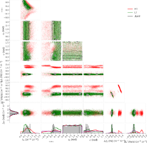
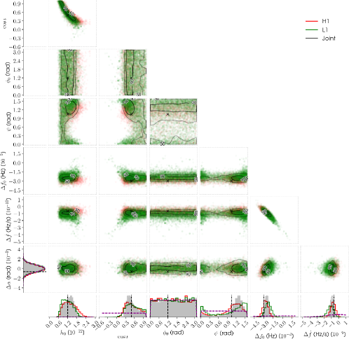
5. Conclusions
In this document we have described some of the workings of a code, lalapps_pulsar_parameter_estimation_nested, that is used for performing parameter estimation and Bayesian model selection in searches for gravitational wave signals from known pulsars. We have described the available signal models, likelihood functions and prior functions. We have compared the code to one that had been previously used for the same purpose, lalapps_pulsar_parameter_estimation, and found that the results agree very well for a range of situations. The comparisons have not been completely exhaustive, and there are situations that have not been tested, however, it is worth noting that lppe is not necessarily expected to provide complete ground truth. The code has also been validated on additional software and hardware simulated signals and appears to return posterior distributions that behave as expected, and evidence values that show the expected behaviour.
As a test of the internal nested sampling algorithm, and proposal distributions, used by the code a large number of simulations were performed using a simple Gaussian likelihood function. These interestingly highlighted that if using, in particular, the ensemble walk proposal distribution the evidence values output became systematically more biased away from the true value as a function of information gain between the prior and posterior distributions. The test showed that this bias was alleviated by including a proposal distribution that drew values from the full prior a certain fraction of the time. The reason for this systematic bias is currently unknown, but in general, given the magnitude of the bias, it should have a relatively minor effect. It was also shown that with the ensemble walk proposal source amplitude upper limits could be systematically biased by about 2%, however, again this effect appears to be alleviated with the flat proposal distribution.
Some example use cases of lppen are documented in Appendix A.
Appendix A Code usage
Here we document the various command line options for the code and its use in a variety of situations. The majority of the command
line options for lppen, as shown with the --help command, are given (in a slightly edited form) in Table LABEL:tab:commands.
| Usage: lalapps_pulsar_parameter_estimation_nested [options] | |
| --help | Display these commands. |
| --verbose | Display progress information from the code, including details of the nested sampling progress. |
| --detectors | Input all interferometers whose data is to be analysed, e.g. H1,L1 (delimited by commas) for the LIGO Hanford and LIGO Livingston detectors (see the discussion in §A.1.4 for the allowed detector names). If generating fake data, described below, these should not be set, otherwise this is required. |
| --par-file | The pulsar’s parameter (.par) file (see §A.1.1). Required. |
| --cor-file | The pulsar’s parameter correlation matrix file (see §A.1.2). Optional. |
| --harmonics | The signal model frequency harmonics that you want to use (delimited by commas). Currently this can be either a single value (e.g., the default is to assume a ’triaxial’ star emitting from the mode and use a value of 2), or 1,2 for a model with emission at both the rotation frequency and twice the rotation frequency. |
| --input-files | The files containing the pre-processed (heterodyned, or spectrally interpolated) data for each detector and model harmonic specified by --detectors and --harmonics delimited by commas (these files must be listed in the same order as passed to --detectors and --harmonics, with the files for different harmonics for individual detectors listed together). If this is not set you can generate fake data (see --fake-data below), but it is otherwise this is required. |
| --outfile | The name for the output data file. This must be a HDF5 file with the extension ’.hdf’ or ’.h5’. Required. |
| --output-chunks | Output lists of the stationary chunks into which the data has been split (see §2.4). Optional. |
| --chunk-min | The minimum stationary length of data to be used in the likelihood. This defaults to 5, e.g., 5 mins for data sampled at 1/60 Hz. Optional. |
| --chunk-max | The maximum stationary length of data to be used in the likelihood. This defaults to 0, which is the value for no maximum length to be applied, except if the --oldChunks flag is set, in which case it defaults to 30. If running with the --roq flag it can be worth setting a value here (e.g., 1440) to avoid large amounts of memory being required in training set generation. Optional. |
| --time-bins | Number of time bins over a sidereal day in the antenna response lookup table. This defaults to 2880 bins. Optional. |
| --prior-file | The file containing the prior ranges for parameters to search over (see §A.1.2). Required. |
| --ephem-earth | The Earth ephemeris file. If not supplied this will attempt to be found in the path. |
| --ephem-sun | The Sun ephemeris file. If not supplied this will attempt to be found in the path. |
| --ephem-timecorr | The Einstein delay time correction ephemeris file. If not supplied this will attempt to be found in the path. |
| --biaxial | Set this if using the waveform model parameters with two harmonics, and specifically for a biaxial star (see, e.g., Pitkin et al., 2015). |
| --gaussian-like | Set this if a Gaussian likelihood is to be used. If the input file(s) contains a column specifying the noise standard deviation of the data then that will be used in the Gaussian likelihood function, otherwise the noise variance will be calculated from the data. |
| --nonGR | Set this to allow non-GR polarisation modes and/or a variable speed of gravitational waves. |
| --randomise | Set this, with an integer seed, to randomise the data (through permutations of the time stamps) for use in Monte-Carlo studies. Note that this will not work if using the code to create injections. |
| --truncate-time | Only analyse data up to the given GPS time. Optional. |
| --truncate-samples | Only analyse data samples up to the number given here. Optional. |
| --truncate-fraction | Only analyse the given fraction of data samples (this must be a value between 0 and 1). Optional. |
| Nested sampling parameters: | |
| --Nlive | Set the integer number of live points for nested sampling. Required. |
| --Nmcmc | Set the length of the MCMC used to find new live points (if not specified an adaptive number of points is used). |
| --Nmcmcinitial | Set the number of MCMC points to use in the initial resampling of the prior. This defaults to 5000, but for our analyses this can be set to zero. |
| --tolerance | The tolerance used as the stopping criterion for the nested sampling integrator. This defaults to 0.1. |
| --randomseed | A seed for the random number generator. By default, if not supplied, this is set by the system clock. |
| MCMC proposal parameters: (see §3.1) | |
| --diffev | The (integer) relative weight of using differential evolution of the live points as the proposal. The default is 0, e.g., 0%. |
| --freqBinJump | The (integer) relative weight of using jumps to adjacent frequency bins as a proposal. The default is 0, and this is not required unless searching over frequency. |
| --ensembleStretch | The (integer) relative weight of the ensemble stretch proposal. The default is 0. Note that this proposal greatly increases the parameter autocorrelation lengths, so in general should be avoided. |
| --ensembleWalk | The (integer) relative weight of the ensemble walk proposal. The default is 3, e.g., 75%. |
| --uniformprop | The (integer) relative weight of uniform proposal. The default is 1, e.g., 25%. |
| Reduced order quadrature (ROQ) parameters: | |
| --roq | Set this flag to use reduced order quadrature to compute the likelihood. |
| --ntraining | The (integer) number of training models used to generate an orthonormal basis of waveform models. |
| --roq-tolerance | The tolerance used during the basis generation. The default is 1e-11. |
| --enrich-max | The (integer) number of times to try and “enrich” (see, e.g., Smith et al., 2016) the basis set using new training data. The enrichment process stops before this value is reached if three consecutive enrichment steps produce no new bases. The default is 100. |
| --roq-uniform | Set this flag to cause training model parameters, for parameters with Gaussian prior distributions, to be drawn from a uniform distribution spanning . Otherwise, by default, parameters are drawn from their given prior distributions. |
| --output-weights | Give an output file name to which to output (a binary version of) the weights will be output. If this is set the programme will exit after outputting the weights. These files could be read in later instead of being regenerated. This allows the potential for the ROQ to be generated on a machine with a large amount of RAM, whilst the full parameter estimation can run on a machine with less RAM. |
| --input-weights | A binary file, created using the --output-weights command, containing all the weights in a defined format. If this is present then the ROQ will not be recalculated. |
| Signal injection parameters: | |
| --inject-file | A pulsar parameter (.par) file containing the parameters of a signal to be injected. If this is given a signal will be injected. |
| --inject-nonGR | A parameter (.par) file containing the values of specific non-GR signal parameters to be injected (this is an alternative to --inject-file, so both should not be passed at the same time). |
| --inject-output | A filename to which the injected signal will be output if specified. |
| --inject-only | If this is set, and an --inject-output file is set, then do not perform nested sampling on the created injection, but just exit the code after creation of, and writing out of, the injection. |
| --fake-data | A list of interferometers for which fake data will be generated, e.g., H1,L1 (delimited by commas). Unless the --fake-psd flag is set the power spectral density for the data will be generated from the noise models in described in §A.1.4. The noise will be white across the data bandwidth. |
| --fake-psd | If wanting to generate fake data with specific power spectral densities for each detector given by --fake-data then they should be specified here delimited by commas (e.g., for --fake-data H1,L1 then you could use --fake-psd 1e-48,1.5e-48) where values are single-sided PSDs in Hz-1. |
| --fake-starts | The start times (in GPS seconds) of the fake data for each detector separated by commas (e.g., 910000000,910021000). If not specified these will all default to 900000000. |
| --fake-lengths | The length of each fake data set (in seconds) for each detector separated by commas. If not specified these will all default to 86400 (i.e., 1 solar day). |
| --fake-dt | The data sample rate (in seconds) for the fake data for each detector. If not specified these will default to 60 s. |
| --scale-snr | This gives a (multi-detector) SNR value to which you want to scale the injection. By default this is 1. |
| Legacy code flags: | |
| --oldChunks | Set this if using fixed chunk sizes for dividing the data as in the old code, rather than the calculating chunks using the change point method. |
| --source-model | Set this if using both 1 and 2 multiples of the frequency and requiring the use of the original source model parameters from Pitkin et al. (2015). |
| Benchmarking: | |
| --time-it | Set this if wanting to time the various parts of the code. A output file with the “outfile” filename appended with “_timings” will contain the timings |
| --sampleprior | Set this to output this (integer) number of samples generated from the prior. The nested sampling will not be performed. |
A.1. Examples
Here we show a few real examples of using the code for a variety of situations. In all cases there are a minimum of three files that must be specified to run the code:
-
1.
One, or more, data files containing a complex time series. These will generally be (although do not have to be) the output of the heterodyne method described in (Dupuis and Woan, 2005) (and implemented with lalapps_heterodyne_pulsar), or the Spectral Interpolation method described in (Davies et al., 2017). Files must be in ascii text format with three, or four, whitespace-separated columns. In either case the first three columns specify the data timestamp in GPS seconds, the real part of the data, and the imaginary part of the data, e.g.,
900000000 1.2564374e-22 -4.5764347e-22. In the case where a fourth column is present this should give the noise standard deviation, and is for use if running with the Gaussian likelihood function. The code will automatically determine if the input contains three or four columns. The data does not have to be uniformly sampled and can contain gaps. However, if searching for a signal for which there could still be some frequency modulation it is useful for the data to have a large enough bandwidth to contain the modulation. The file can contain comments if the a line starts with a%or#. Gzipped versions of these files can also be input. -
2.
A pulsar parameter file. This should be an ascii text tempo(2)-style
.parfile containing information on the source’s parameters, e.g. sky location and frequency, as generated by tempo222222http://tempo.sourceforge.net/ or tempo2 (Hobbs et al., 2006) from pulsar pulse time-of-arrival observations. An example.parfile is given below. -
3.
A prior distribution file. This should be an ascii text file containing information on the prior distributions required for any variable parameters for which the code needs to sample posterior probability distributions. An example prior file is given below.
In the examples below we will assume that the LALSuite software package (LIGO Scientific Collaboration, 2017) has been installed and that the executable binaries for lppen and lalapps_nest2pos are in your path (i.e. the directory path containing those executables is set in the list of values in your PATH environment variable). The code can automatically find solar system ephemeris and timing files provided they are in a standard location, although these can also be specified explicitly on the command line.
A.1.1 An example .par file
The .par file input should be the same file that was used when performing the heterodyning (or Spectral Interpolation)
of the data used to produce the input data time series. A tempo(2)-style .par file could have the following form, e.g.,
for a pulsar in a binary system:
⬇
PSRJ J0234+5612
RAJ 02:34:12.123485
DECJ 56:12:05.237474
F0 102.764742743786 1 1.2341e-10
F1 -8.854276e-14
PEPOCH 54012.2853
BINARY BT
ECC 0.023
T0 53424.24435856
OM 12.858534
PB 9.858345
A1 3.474743
The majority of the parameters that can be in a .par file are listed in Table A1 of Edwards et al. (2006). Note that our code does not compute effects of dispersion measure (i.e. it assumes observations at infinite frequency), or atmospheric effects, so it is preferable to use a .par file for which these parameters have been not used, or held fixed.
For pulsars in binary systems, the code can currently use the following binary system models (see, e.g., Taylor and Weisberg, 1989; Pitkin and Woan, 2007, for discussion of some of the models): BT, BTX, BT1P, BT2P, ELL1, DD, DDS, MSS, and T2 (although not all aspects of the T2 model are implemented). The code can use the TDB or TCB time systems, with the TCB system being the default if not otherwise specified (either by supplying the require timing files, or by setting “UNITS TDB” in the .par file). The code can accept .par files calculated using the JPL DE200, DE405, DE414, or DE421 solar system ephemerides, noting that it only takes into account the motion of the Earth-Moon system and the Sun, but no other solar system bodies.
The .par file can also contain a selection of gravitational wave parameters not present in the case of a standard electromagnetically observed pulsar. A full list of the allowed parameter names for a .par, and a prior file described below, is given in Table LABEL:tab:paramlist.
| Parameter | Description |
| Gravitational wave parameters | |
| H0, | gravitational wave amplitude for the mode in the source model (see, e.g., Jaranowski et al., 1998) |
| IOTA, | pulsar inclination angle to the line-of-sight (rads) ( is gives a source whose rotation axis is pointed directly along the line-of-sight) |
| COSIOTA, | cosine of |
| PSI, | polarisation angle of the gravitational waves (rads) (see, e.g., Jaranowski et al., 1998) |
| PHI0, | rotational phase of the pulsar (rads) |
| C22, | gravitational wave amplitude for the mode in the waveform model (see Pitkin et al., 2015) |
| C21, | gravitational wave amplitude for the mode in the waveform model (see Pitkin et al., 2015) |
| PHI22, | gravitational wave phase for the mode in the waveform model (rads) (see Pitkin et al., 2015) |
| PHI21, | gravitational wave phase for the mode in the waveform model (rads) (see Pitkin et al., 2015) |
| Q22, | mass quadrupole moment (kg m2) (see e.g. Owen, 2005) |
| I21, | physical gravitational wave amplitude in source model (see Pitkin et al., 2015) |
| I31, | physical gravitational wave amplitude in source model (see Pitkin et al., 2015) |
| LAMBDA, | Euler angle in source model (see Pitkin et al., 2015) |
| THETA, | Euler angle in source model (see Pitkin et al., 2015) |
| COSTHETA, | cosine of |
| Signal phase parameters | |
| F, | rotational frequency, and frequency derivatives (starting at 0), (Hz) |
| PEPOCH | the epoch of the frequency (MJD, defined in the inertial frame of the pulsar, with often this being the solar system barycenter) |
| Signal positional parameters | |
| RA/RAJ, | pulsar right ascension (hh:mm:ss.s) |
| DEC/DECJ, | pulsar declination (dd:mm:ss.s) |
| PMRA | proper motion in right ascension (mas yr-1) |
| PMDEC | proper motion in declination (mas yr-1) |
| POSEPOCH | the epoch of the sky position (MJD) |
| EPHEM | the JPL solar system ephemeris |
| PX | pulsar parallax (mas) |
| DIST | pulsar distance (kpc) |
| Binary system oribital parameters | |
| BINARY | binary system model (see e.g. Taylor and Weisberg, 1989, and references therein) |
| A1, | projected semi-major axis (lt-s) |
| PB, | binary period (days) |
| OM, | longitude of periastron (degs) |
| T0 | time of periastron (MJD) |
| ECC, | orbital eccentricity |
| EPS1, / | for ELL1 model (see Appendix in Lange et al., 2001) |
| EPS2, / | for ELL1 model (see Appendix in Lange et al., 2001) |
| TASC, | time of the ascending node for ELL1 model (see Appendix in Lange et al., 2001) |
| GAMMA, | relativistic gravitational redshift and time dilation term in BT model (s) |
| OMDOT, | time derivative of (degs yr-1) |
| XDOT | time derivative of (lt s s-1 or lt-s s-1 if ) |
| PBDOT, | time derivative of period ( if ) |
| EDOT, | time derivative of eccentricity (s-1 or s-1 if ) |
| EPS1DOT, | time derivative of (s-1 or s-1 if ) |
| EPS2DOT, | time derivative of (s-1 or s-1 if ) |
| XPBDOT | time derivative of period minus GR prediction ( if ) |
| SINI, | sine of orbital inclination angle |
| MTOT, | total binary system mass (M⊙) |
| M2, | binary companion mass (M⊙) |
| DR, | relativistic deformation of the orbit |
| DTHETA, | relativistic deformation of the orbit |
| SHAPMAX, | defined as |
| KOM, | longitude of ascending node (Kopeikin term) (degs) |
| D_AOP | Kopeikin term (arcsec-1) (see, e.g., Section 2.7.1 of Edwards et al., 2006) |
| A1_ | projected semi-major axes for multiple orbital components ( for BT1P and BT2P models) (lt-s) |
| PB_ | periods for multiple orbital components ( for BT1P and BT2P models) (days) |
| OM_ | longitudes of periastron for multiple orbital components ( for BT1P and BT2P models) (degs) |
| T0_ | times of periastron for multiple orbital components ( for BT1P and BT2P models) (MJD) |
| ECC_ | eccentricities for multiple orbital components ( for BT1P and BT2P models) |
| FB | orbital frequencies for multiple components (in BTX model) (Hz) |
| A0, | first aberration parameter (see, e.g., Section 2.7.3 of Edwards et al., 2006) |
| B0, | second aberration parameter (se, e.g., Section 2.7.3 of Edwards et al., 2006) |
| Glitch parameters (see Hobbs et al., 2006; Yu et al., 2013) | |
| GLEP_ | glitch epochs (MJD) |
| GLPH_ | glitch rotational phase offsets (rads) |
| GLF0_ | glitch frequency offsets (Hz) |
| GLF1_ | glitch first frequency derivative offsets (Hz s-1) |
| GLF2_ | glitch second frequency derivative offsets (Hz s-2) |
| GLF0D_ | glitch decaying frequency components (Hz) |
| GLTD_ | glitch time constant for decaying components (s) |
| Non-GR parameters | |
| CGW, | speed of gravitational waves as a fraction of the speed of light |
| HPLUS, | gravitational wave amplitude for the tensor -polarisation (see, e.g., Isi et al., 2017, for definitions of this and the subsequent parameters) |
| HCROSS, | gravitational wave amplitude for the tensor -polarisation |
| PHI0TENSOR, | tensor mode phase parameter |
| PSITENSOR, | tensor mode phase parameter |
| HVECTORX, | gravitational wave amplitude for the vector x-polarisation |
| HVECTORY, | gravitational wave amplitude for the vector y-polarisation |
| PHI0VECTOR, | vector mode phase parameter |
| PSIVECTOR, | vector mode phase parameter |
| HSCALARB, | gravitational wave amplitude for the scalar -polarisation |
| HSCALARL, | gravitational wave amplitude for the scalar -polarisation |
| PHI0SCALAR, | scalar mode phase parameter |
| PSISCALAR, | scalar mode phase parameter |
A.1.2 Example prior file
The prior functions used by the code are described in §2.3. To implement them in the code requires a prior file specifying the prior function require for each parameter that will be varied. A an example prior file containing all the allowed prior types (for descriptive purposed only) is:
The units required for parameters in a prior file are all SI units, whereas for the .par file they often follow a different convention (see Table LABEL:tab:paramlist).
Going through each line we have:
- H0
-
this parameter has been assigned a Fermi-Dirac prior (§2.3.5) using the fermidirac tag, which requires two values: and .
- PHI0
-
this parameter has been assigned a uniform prior (§2.3.1) using the uniform tag, which requires two values: a lower limit and an upper limit.
- PSI
-
this parameter has been assigned a Gaussian prior (§2.3.2) using the gaussian tag, which requires two values: a mean and a standard deviation.
- A1
-
this parameter has been assigned a prior uniform in the logarithm of the parameter (§2.3.4) using the loguniform tag, which required two values: a lower limit and an upper limit on the parameter (not the logarithm of the parameter).
- F0:F1
-
this pair of parameters has been assigned a Gaussian mixture model prior (§2.3.3). This prior can be used for any number of parameters if given as a colon separated list in the prior file. Following the gmm assignment, a number gives the number of modes for the model. This is then followed by a square-bracketed list of lists, with each mode giving a comma separated main list entry containing a sub-list of comma separated means for each parameter (no additional whitespace is allowed in the lists). The list of means is then followed by a similar list of parameter covariance matrices for each mode (again no additional whitespace is allowed). This is then followed by a final bracketed list giving the relative weights for each mode (the weights do not have to be normalised to unity, as the code will automatically normalise them). If required this can then be followed by pairs of bracketed, comma separated values, for each parameter giving their minimum and maximum allowed ranges. If these are given then they have to be given for all parameters, not just some subset. These are not shown in this example.
- COSIOTA
-
this single parameter has been assigned a Gaussian mixture model prior (§2.3.3). This shows how to input a Gaussian mixture mode for a single parameter, and also shows at the end minimum and maximum ranges for the parameter have also been input.
If parameters in the prior file are specified with the gaussian tag then a multivariate Gaussian prior may also be used for them if a correlation matrix
is passed to lppen (using the --cor-file flag) containing correlation coefficients for the required parameters. Only the lower diagonal of the
correlation matrix is required, e.g. if we wanted a multivariate prior on and we could have a correlation coefficient file containing:
⬇
F0 F1
F0 1
F1 0.5 1
where the whitespace can be tabs or spaces, whilst the prior file contains the means and standard deviations of the parameters as noted above. It is worth noting
that, for fully (anti)correlated parameters correlation coefficients of one can lead to numerical issues during matrix inversion. So, in such cases the
(anti)correlation could be reduced to, say, 99.99%. However, better solutions to such a degeneracy would be to fix one of the correlated values (i.e. do not include
it in the prior file) and only searching over the other, or finding a non-degenerate re-parameterisation.
A.1.3 Example 1: single detector, single harmonic, input data
One of the simplest cases for running the code is on input data from a single detector and at a single frequency harmonic (in this
case at twice the rotation frequency). Let us assume a search that is just interested in a signal model described by the four parameters
, , and , and set a prior file, called prior.txt, containing
⬇
H0 uniform 0 1e-20
PHI0 uniform 0 3.14159265359
PSI uniform 0 1.57079632679
COSIOTA uniform -1 1
Given a pulsar .par file, called, for example, pulsar.par containing232323For a search that does not include any phase evolution parameters
the only required values in the .par file are the right ascension and declination, but in general the file passed to the code should be the one used
to perform the heterodyning that produced the input data file.
⬇
PSRJ J1234+5601
RAJ 12:24:00.00
DECJ 56:01:00.00
F0 100.01
F1 -1.1e-10
PEPOCH 56789
EPHEM DE405
and assuming the input data (from the LIGO Hanford detector, H1, in this case) is in a file called data_H1.txt, then one would run:
where we have set an output HDF5-format file called nest_H1.hdf in which the nested samples will be output. This setup has used 1024 nested sampling live points and a tolerance of 0.1 for stopping the code. The --Nmcmcinitial 0 flag tells the code that the initial live points drawn do not have to be resampled.242424This option is present for cases when the initial live points may not be easily sampled from their prior distributions, and therefore an MCMC procedure is required to try and evolve them to be drawn from the actual prior. However, for all our priors there are simple ways to draw the initial live points from the prior, so this resampling is not required, and this input argument can be set to zero. In this case the solar system ephemeris files will be found automatically. If the EPHEM or UNITS parameters are not explicitly set in the .par file then these will default to the DE405 ephemeris and the TCB time system. The progress of the above code can be monitored by including the --verbose flag, and watching how the reported dZ value approaches the required tolerance.
Along with the file of nested samples two additional files called nest_H1_SNR and nest_H1_Znoise will be output. The former contains the recovered optimal SNR for the maximum likelihood sample. The later contains the null likelihood, or noise, evidence for the data, described in §2.2.3. The noise evidence is also contained in the nest_H1.hdf file, but this additional file is useful in cases when multiple harmonics are used as it will contain noise evidences for individual harmonic datastreams, as well as that for the multiple combined streams.
The nested sample file can be converted to a file containing posterior samples, called, say, post_H1.hdf, using:
⬇
$ lalapps_nest2pos -p post_H1.hdf nest_H1.hdf
where the -p flag give the name of the posterior output file. If the above use of lppen had been run more than once on the same data and prior file,
with output names given by e.g. nest_H1_01.hdf…nest_H1_.hdf, then all these could be listed as input to lalapps_nest2pos to
combined all the samples and evidence estimates. As well as the posterior samples, this file also contains (as does the nest_H1.hdf),
the signal model evidence, the noise model evidence, and the information gain (amongst other things).
The posterior samples, and noise and signal model (natural logarithm) evidences, can be extracted using a python function within lalapps, via
⬇
$ python
>>> from lalapps import pulsarpputils as pppu
>>> postsamples, sigevidence, noiseevidence = pppu.pulsar_nest_to_posterior(’post_H1.hdf’)
The postsamples variable is an object from which samples from different parameters can be extracted, and plotted as a marginalised posterior
distribution, e.g.,
⬇
>>> from matplotlib import pyplot as pl
>>> # plot the posterior samples for the H0 parameter
>>> pl.hist(postsamples[’H0’].samples, bins=20, normed=True, histtype=’stepfilled’)
>>> pl.xlabel(’$h_0$’)
>>> pl.ylabel(’Posterior Probability Density’)
>>> pl.show()
where here, for the parameter it is contained in postsamples as the fully uppercase ’H0’ value.
Alternatives to extract the (natural logarithm) evidence values are using the h5py python module, or HDF5 command line utilities. For the former one could
use, e.g.,
⬇
>>> import h5py
>>> hdf = h5py.File(’post_H1.hdf’, ’r’)
>>> a = hdf[’lalinference’][’lalinference_nest’]
>>> sigevidence = a.attrs[’log_evidence’]
>>> noiseevidence = a.attrs[’log_noise_evidence’]
>>> information = a.attrs[’information_nats’]
or for the latter one could use, e.g.
⬇
$ h5ls -v post_H1.hdf/lalinference/ | grep -A2 evidence
Attribute: log_evidence scalar
Type: native double
Data: 141816
--
Attribute: log_noise_evidence scalar
Type: native double
Data: 141822
However, note that in this latter example the evidence values are truncated to integer values.
A.1.4 Example 2: single detector, single harmonic, simulated data
As well as taking real data as an input the code can simulate Gaussian noise, and/or create and add a simulated signal to the data. To create
a signal to inject into the data requires a .par file for the injected signal parameters. This can be the same, or different, to the file input
using the --par-file flag, but to produce a non-zero signal it must contain at least a gravitational wave amplitude parameter (any parameters not
included will be assumed to be zero). Any differences in the phase evolution parameters between the two files will be incorporated into the
signal via Equation 10. Given an injection .par file, called, say, injection.par, containing
⬇
PSRJ J1234+5601
RAJ 12:24:00.00
DECJ 56:01:00.00
F0 100.01
F1 -1.1e-10
PEPOCH 56789
EPHEM DE405
H0 1e-25
COSIOTA -0.43
PHI0 0.6
PSI 1.2
(which we see is the same as in §A.1.3, but with gravitational wave amplitude parameters), one would run the following (assuming various other
names are the same as in §A.1.3)
Here, rather than inputting a real data file, the --fake-data flag has been used to specify fake data from the LIGO Hanford detector, where the
design sensitivity (Lazzarini and Weiss, 1996)252525https://labcit.ligo.caltech.edu/~jzweizig/distribution/LSC_Data/ power spectral density noise curve
would be used to set the Gaussian noise level for an initial LIGO detector at the appropriate gravitational wave frequency (twice the value of F0 given in the .par
file for the standard search).262626Other
named detectors that can be provided are L1 for the LIGO Livingston detector, G1 for the GEO600 detector (from Table IV of Damour et al., 2001),
V1 for the initial Virgo detector, and T1 for the TAMA300 detector (from Table IV of Damour et al., 2001). For the two LIGO detectors
(Shoemaker, 2009) and Virgo (see Equation 6 of Manzotti and Dietz, 2012), design curve noise levels for their Advanced configurations can be obtained
by prefixing the names with an ‘A’. Setting the noise level from the design sensitivity for a given detector can be overridden by also using the
--fake-psd flag to input the required single sided power spectral density value. The simulated data will by default start at a GPS time of 900000000
(13 Jul 2088, 15:59:46 UTC), be sampled at a rate of once per minute, and last for one solar day. However, each of these can be set with the appropriate flags:
--fake-starts, --fake-lengths, and --fake-dt, respectively. In this example a value is also set for --scale-snr, which means that after the
creating of a signal with parameters as given in the injection.par file, it will be re-scaled so that it has the given SNR - in this case a value of 10. This
enables signals to be injected with a known SNR without needing to know the noise level a priori. If the --scale-snr flag is not set, or has a value of zero,
then no re-scaling takes place. In this case the output nest_H1_SNR file would also contain the signal’s injected SNR and the recovered SNR, e.g.,
⬇
$ cat nest_H1_SNR
# Injected SNR
H1 2.000 2.642255e+01 1.000000e+01
# Recovered SNR
H1 2.000 1.092211e+01
where, after the detector name the harmonic frequency scaling factor is given, and for the injected signal the two SNR values are the pre-scaled value
and the actually injected value after rescaling via --scale-snr value.
A simulated signal can also be injected into real data in the same way.
A.1.5 Example 3: multiple detectors, single harmonic
Running with multiple detectors requires a simple change to the example given in §A.1.3. Given two input files, e.g. data_H1.txt and data_L1.txt, for the two LIGO detectors H1 and L1, one would simply use, e.g.
where the order of listing the detectors with the --detectors flag should match the order of listing the data files with the --input-files flag. No whitespace is allowed between detector values or input file values, and they must be separated by a comma. In this case the output nest_H1L1_SNR file will contain the individual detector recovered SNRs and the coherent SNR, whilst the nest_H1L1_Znoise file will contain both the individual detector noise model evidences and the combined noise model evidence.
A.1.6 Example 4: multiple detectors, two harmonics
It is simple to extend the analysis to include the two harmonics from the mode (with a gravitational wave frequency at twice the rotation rate) and the ,
harmonic (with a gravitational wave frequency at the rotation rate). To search at these two harmonics requires that the parameters searched over are either the signal or
waveform parameters given in Pitkin et al. (2015). Using the (simpler and non-degenerate) waveform parameters , , and
, from Equations 7 and 8, could lead to the following (prior.txt) prior file
⬇
C22 uniform 0 1e-20
C21 uniform 0 1e-20
PHI22 uniform 0 6.28318530718
PHI21 uniform 0 6.28318530718
PSI uniform 0 1.57079632679
COSIOTA uniform -1 1
Assuming that for each detector (H1 and L1) the data has been heterodyned at both harmonics, leading to files data_H1_1f.txt, data_H1_2f.txt,
data_L1_1f.txt, data_L1_2f.txt, where 1f and 2f note the harmonic rotation frequency scaling, then one would use
Here the ordering of the input files is important, with the files for each harmonic for a given detector listed together, and in the same order as given by the --harmonics flag. The noise evidence and SNRs for each harmonic and each detector will be output to the files nest_H1L1_Znoise and nest_H1L1_SNR.
A.1.7 Example 5: single detectors, additional parameters
Finally, we show an example when searching over additional phase evolution parameters. We show two options for this: the first is using the standard
model and likelihood method, and the second performs the same search, but sped-up by using the ROQ likelihood. If one were searching over frequency and
frequency derivative, and , then an example .par file (pulsar.par) could be
⬇
PSRJ J1234+5601
RAJ 12:24:00.00
DECJ 56:01:00.00
F0 100.01
F1 -1.1e-10
PEPOCH 54660
EPHEM DE405
with a prior file (prior.txt) containing
⬇
H0 uniform 0 1e-20
PHI0 uniform 0 3.14159265359
PSI uniform 0 1.57079632679
COSIOTA uniform -1 1
F0 gaussian 100.01 1e-5
F1 gaussian -1.1e-10 2e-11
Note that the frequency and frequency derivative values in the prior file are for the rotation frequency, so if searching for the standard
harmonic then the actual frequencies and derivatives (and in this case their standard deviation) covered will be twice these values. This would also
be the case for any other form of the prior. As, in this example, the F0 and F1 values have be assigned Gaussian priors, if they have a
known correlation then a correlation coefficient file (pulsar.cor) could also be set, e.g.
⬇
F0 F1
F0 1.0
F1 0.7 1.0
However, if this is not provided, then the parameters will be assumed to a priori be uncorrelated.
If running without ROQ, for a data from a single detector, H1 (data_H1.txt), the following commands could be used
To run with ROQ enabled, in the simplest case, requires the user to set a number of training waveforms and tolerance to use the produce a reduced order model.272727For now we do not attempt to explain these parameters, which we are leaving to a future publication, other than to say that for broader parameter space searches (or searches over frequency derivatives, for which the epoch is further from the data epoch) more training waveforms are required for a given tolerance. For a fixed tolerance, if the parameter space is too broad more templates may be required than are computational feasible (due to, e.g., memory constraints) to use. In this example we will use 2500 training waveforms, and a tolerance of , and use data that starts at the same epoch as given in the .par file. The following commands could be used
In this example, for a single run on a random realisation of Gaussian noise lasting one day and sampled at a rate of one per minute, we find that the ROQ version runs about 1.8 times faster. Within the given tolerance it reduces the prior parameter space to 32 orthogonal waveform templates, thus reducing the the model and likelihood evaluations from using 1440 to 32 points. Due to various overheads the speed-up we see between the ROQ and regular run is only a factor of , rather than the factor that might be hoped for. However, more impressive speed-up can be observed for longer data sets. It should be noted that this observed speed-up is not a general rule, but is specific to the data and set up we used, but similar speed-ups for similar set ups would not be unexpected. We also find that the likelihoods produced by the ROQ method agree very well with that produced using the full likelihood evaluation, with the maximum-likelihood-template likelihoods agreeing to within .
A.1.8 Example 6: single detector, non-GR model
The standard analysis considers two hypotheses: GR signal and Gaussian noise. On top of these, we can also include non-GR signal hypotheses consisting of all possible combinations of tensor, vector and scalar modes: GR+s, GR+v, GR+sv, s, v, sv (see Isi et al., 2017, for definitions of these).282828If the orientation of the source is known, we can also make a distinction between GR and a “free-tensor” hypothesis, corresponding to a signal model with and polarisations with unrestricted amplitudes and phases. For any set of data, we can compute Bayes factors for each of these hypotheses using lppen and then combine them to produce odds for any-signal vs. noise and non-GR vs. GR.
The lppen code accepts the --nonGR and --inject-nonGR arguments, which can be used to search for and inject non-GR signals, respectively. Both options may be used as simple flags or with a specific argument. In the former case, the code will use a generic signal model that includes all polarisations mentioned in the prior file. For instance, for a single detector (H1 in this case) the most generic search (one including all 5 non-degenerate polarisations freely) would be carried out by calling (without injections):
with a prior file like:
⬇
HPLUS loguniform 1e-28 1e-21
HCROSS loguniform 1e-28 1e-21
PHI0TENSOR uniform 0 6.283185307179586
PSITENSOR uniform 0 6.283185307179586
HVECTORX loguniform 1e-28 1e-21
HVECTORY loguniform 1e-28 1e-21
PHI0VECTOR uniform 0 6.283185307179586
PSIVECTOR uniform 0 6.283185307179586
HSCALARB loguniform 1e-28 1e-21
PHI0SCALAR uniform 0 6.283185307179586
where HPLUS and HCROSS are the tensor amplitudes, HVECTORX and HVECTORY are the vector amplitudes and HSCALARB is the scalar amplitude
(we could equivalently use HSCALARL, since the breathing and longitudinal modes are degenerate to quadrupolar antennas like LIGO or Virgo); the PHI0TENSOR,
PHI0VECTOR and PHI0SCALAR parameters determine the overall complex phase offset between different ranks, while PSITENSOR and PSIVECTOR are
phase offsets between modes of the same rank. Relevant parameters that do not explicitly show up in the prior file are set to zero; as a result, the same command above
can be used to search only over, say, vector modes by changing the prior file to read:
⬇
HVECTORX loguniform 1e-28 1e-21
HVECTORY loguniform 1e-28 1e-21
PHI0VECTOR uniform 0 6.283185307179586
PSIVECTOR uniform 0 6.283185307179586
This can be used to produce any of the “free” non-GR searches (s, v, t, sv, st, vt, svt). Note that, if any of the prior files are used without the --nonGR
flag, the code will fail, as it will expect GR-specific parameters (like H0 and COSIOTA). A generic non-GR injection may be produced by using the
--inject-nonGR flag with an injection file that gives the values of non-GR parameters desired, e.g.,
⬇
HPLUS 3e-24
HVECTORX 4e-24
PHI0VECTOR 3
would produce an injection with ‘+’ and vector-x components of the given strain amplitudes, with no phase offset for plus (PHI0TENSOR is 0) and 3 radians for
vector-x.
The non-GR options also accept an argument that specifies a particular non-GR model; currently accepted options are G4V and EGR. The former corresponds
to a vector-only model (proposed in Mead, 2015) that we usually use for testing; this model includes vector x and y modes with a particular
weighting given by the pulsars inclination as in equations 7 and 8 of Isi et al. (2015). An example of a prior file for a --nonGR G4V analysis
would be:
⬇
PSI uniform -0.785398163397448 0.785398163397448
IOTA uniform 0 6.283185307179586
H0 loguniform 1e-28 1e-21
PHI0VECTOR uniform 0 6.283185307179586
The second option accepted by --nonGR and --inject-nonGR is EGR, which stands for “enhanced GR”. This corresponds to a model made up of a GR signal
(parametersied in the usual way by , , and ) plus contributions from any non-tensorial modes specified in the prior file. For instance, passing --nonGR EGR with a prior like:
⬇
PSI uniform -0.785398163397448 0.785398163397448
COSIOTA uniform -1 1
H0 loguniform 1e-28 1e-21
PHI0TENSOR uniform 0 6.283185307179586
HVECTORX loguniform 1e-28 1e-21
HSCALARB loguniform 1e-28 1e-21
PHI0SCALAR uniform 0 6.283185307179586
will produce a GR+s search; thus, by appropriately modifying the prior file, the --nonGR EGR option can be used to also search for GR+v and GR+sv signals.
Non-GR injection files are constructed similarly.
A.2. The pipeline
The process of performing searches for known pulsars does not just use lppen. It actually requires a whole pipeline of code to: a) gather the gravitational wave detector data and operational segments (“science mode”); b) pre-processing the raw data via heterodyning (or spectral interpolation) to give the complex down-sampled time series; c) set up the required prior distribution files; d) pass the data and priors to lppen; e) convert the output nested samples into posterior samples; and, finally, f) display those results (including odds values) in a useful fashion, e.g. on a webpage. This process can be performed manually in a step by step manner, but there also exists a pipeline script called lalapps_knope that gathers together all these operations in a way that can be run on a computer cluster running the HTCondor292929https://research.cs.wisc.edu/htcondor/ job management system.
To run this pipeline requires just a single configuration file to be written in the INI303030https://en.wikipedia.org/wiki/INI_file format. An example configuration file is given below containing comments on the necessary input fields:
Unless specified as otherwise within a .par file the pipeline assumes the use of the TCB timing convention (as is the default for TEMPO2), and the DE405 solar system ephemeris.
Appendix B Derivation of the Student’s t-likelihood function
Here we derive, in detail, the form of the Student’s t-likelihood given in Section 2.2. This derivation can, in part, be found in Dupuis (2004) and Dupuis and Woan (2005), but we correct a slight error from those references.
If a stretch of data of length is assumed to consist of a signal defined by a set of parameters and Gaussian noise with zero mean and standard deviation , then the standard deviation can be included as an unknown parameter in the likelihood function and marginalised over. The likelihood can therefore be given by
| (B1) |
where is the likelihood function for the data given the unknown signal parameters and the noise standard deviation, and is the prior on .
Given that the noise is assumed Gaussian the likelihood within the integral is given by
| (B2) |
for our complex data and model , where for a complex number we have used , and the noise in the real and imaginary parts is assumed to have the same distribution.
We chose a scale invariant prior on of , for which the marginalisation of Eqn. B1 can be performed analytically as we will show. Substituting this prior and Eqn. B2 into Eqn. B1 we can begin the integration with the substitution
| (B3) |
giving
| (B4) |
Here we note that Eqn. B4 is different from the equivalent Eqn. 2.28 in Dupuis (2004) by a factor of two. Rearranging Eqns. B3 and B4, and for simplicity using the substitution , gives
| (B5) |
and
| (B6) |
Putting everything into Eqn. B1 gives
| (B7) |
The integral in Eqn. B can then be performed by making the substitutions and , giving
| (B8) |
This integral is the definition of the Gamma function
| (B9) |
For positive integers, Stirling’s formula shows that the Gamma function is given by , so our likelihood becomes
| (B10) |
Note that, again, this differs from Eqn. 2.31 in Dupuis (2004) by some constant factors.
For our analysis the data is split into chunks for each of which the assumption of noise stationarity is thought to be valid, but between chunks is thought to be invalid (see discussion in §2.4). The joint likelihood of all data can be obtained from the product of the likelihood for each chunk given by
| (B11) |
where is the total number of independent data chunks with lengths and (with ) is the index of the first data point in each chunk.
Appendix C Fast likelihood evaluation
In §2.2.4 we stated that the likelihood can be evaluated quickly in cases where the values in Equations 7, 8 and 11 are zero, i.e., no phase evolution parameters are required. This can be done by pre-summing over data, , and combinations of the time-varying antenna response function, after which only coefficients of these pre-summed terms need to be calculated. Here we will explicitly write out the derivation of these coefficients for the case of a signal in GR, for which the antenna pattern functions for the ‘’ and ‘’ components are given by Equation 2.2.4.
Assuming a signal in GR, we start with a model of the form
| (C1) |
where, setting in Equation 2.2.4, the antenna pattern functions are
| (C2) |
and we have set the real and imaginary model amplitude coefficients for the two polarisations to be , , , .313131For our GR signal model emitting at twice the rotation frequency, given by Equation 8, we would have and . If we just take the likelihood (either the Student’s -likelihood of Equation 2.2.1, or the Gaussian likelihood of Equation 2.2.2)323232If using the Gaussian likelihood there is a slight difference to what is described here to take account of the data noise standard deviation, , such that we require the substitutions , and . for a single detector, data stream, and data chunk (see §2.2) then we see that it contains the summation over time samples
| (C3) |
We can expand this out to give
| (C4) |
where for convenience we have removed the summation subscripts and explicit time dependence, and used and subscripts to represent the real and imaginary components respectively. We are now interested in the summations that contain parts of the model function . If we take the summation over the square of the real part of the model we get
| (C5) |
where the summation is now implicit in the and terms, i.e., , , and , which are the only time varying components and can be pre-computed. If we now say
| (C6) |
where the s are the coefficients of , and , we find them to be
| (C7) |
Factorising these out we find that
| (C8) |
where , , and . It is easy to see from above that things will be identical for the imaginary components and the equations hold just by swapping for . It is worth noting that the coefficients given in Equation C take the opposite form (covariant vs. contravariant rotation) than the antenna pattern functions given in Equation C, and this difference is present in the model in the lppen code, but should not be unexpected.
We can also see that the coefficients given in Equation C are those required in the components of Equation C that sum over the product of the data and model. For the real part we have
| (C9) |
where we have set and . We can therefore see that the coefficients of and are indeed and respectively, i.e.,
| (C10) |
Again, this holds for the imaginary parts by just swapping for .
The same process can be applied for likelihood evaluations for the non-GR polarisation modes. For the ‘x’ and ‘y’ modes the antenna patterns can be defined as (Equations 32 and 33 of Isi et al., 2015)
| (C11) |
In this case we find, in an identical fashion to above, that the required coefficients of and are
| (C12) |
where are the real/imaginary signal amplitude components for the two modes. Finally, for the breathing and longitudinal modes, where the antenna patterns are defined as (Equations 34 and 35 of Isi et al., 2015)
| (C13) |
and there is no dependence, the coefficients of and are just the real/imaginary signal amplitude coefficients for the modes.
Appendix D Relation between odds and SNRs
It is interesting to look at how we might expect odds values (ratios of evidences) to vary with signal-to-noise ratio (SNR) (also see similar discussions in Isi et al., 2017). We will take the simple case of two Gaussian datasets both of the same length () and standard deviation, . Both datasets contains a mean offset of , and we are concerned with a search over the mean parameter. We want to calculate two things: the odds for a mean offset versus the data being Gaussian noise with a known mean of zero; and, the odds for both datasets containing the same mean offset (a coherent signal) versus them containing two independent mean offsets (an incoherent signal). We can try and work out what to expect using approximations, and then see if that’s actually the case when calculating the values analytically.
To set up the situation, we have the two datasets and , which have likelihoods given by
| (D1) |
and priors on given by , which we will take as constant (i.e. a flat prior). We will also use the fact that where is a value drawn from a Gaussian distribution of zero mean and standard deviation , and is the true offset.
To re-cap from earlier in this paper, the evidence is given by
| (D2) |
for hypothesis .
D.1. Coherent signal vs. noise odds
For large SNRs the relation between signal () versus noise () evidence odds for Gaussian noise is well known, but we’ll write it out explicitly here. Formally, for our two data steams, we have
| (D3) |
For high SNR signals the we find that
| (D4) |
where is the likelihood at the true/maximum likelihood value of . This value, for the joint datasets, can be seen to be
| (D5) |
which in turn (with ) becomes
| (D6) |
where we have used . Similarly, we have the noise evidence
| (D7) |
where we use the approximation that . So, the odds becomes
| (D8) |
where we can also say that the single dataset SNR is defined as , and in this case , and we can see that if we take the natural logarithm of this that
| (D9) |
We see here that the log odds is proportional to , with a minor influence from the term which is roughly equivalent to . Empirically (and probably with some mathematical justification that can be derived) this approximation seems to give the median odds value on random realisations of noise, even down to low SNR (see Figure 34).
D.2. Coherent signal vs. incoherent signal
We can define a coherent signal versus incoherent signal odds ratio as
| (D10) |
where , , and , are the evidences for a signal in the full dataset, and two individual datasets (this is equivalent to Equation 2.6). Using the same approximations as above, we find that
| (D11) |
In this we see that there is the Occam factor of accounting for the fact that the incoherent model has an extra parameter. We also see that this is proportional to which is roughly equivalent to .
So we see that for the coherent signal versus noise odds roughly scales with , whilst the coherent signal versus incoherent signal odds roughly scales with , i.e. its scaling is a lot shallower. Empirically (and probably with some mathematical justification that can be derived) this approximation seems to give the maximum odds value on random realisations of noise down to low SNR (see Figure 34).
In Figure 34 we see how these two approximations compare to analytical calculations of the odds values as the SNR changes. For a range of SNRs we created multiple realisations of two dataset of Gaussian random noise (with SNR altered by altering the standard deviation of the noise) with a given mean offset. In each case we have analytically calculated the evidences for a coherent for both datasets, and independent in both datasets. These are then compared to the approximations above. In this case we have purposely chosen a prior on such that the distributions of odds values for and cross, which is similar to the case we observed in our actual analysis shown in §4.1.2.
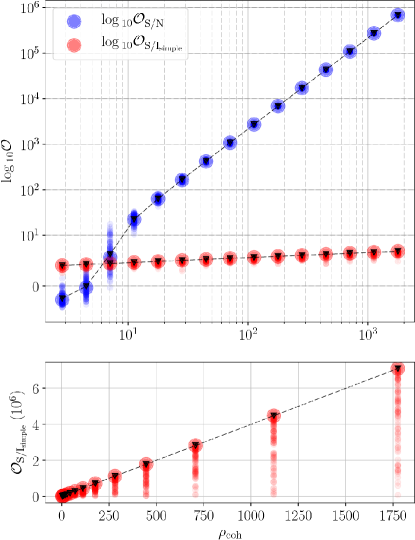
References
- Aasi et al. (2015) J. Aasi, B. P. Abbott, R. Abbott, et al., Classical and Quantum Gravity 32, 074001 (2015), arXiv:1411.4547 [gr-qc] .
- Acernese et al. (2015) F. Acernese, M. Agathos, K. Agatsuma, et al., Classical and Quantum Gravity 32, 024001 (2015), arXiv:1408.3978 [gr-qc] .
- Abbott et al. (2016a) B. P. Abbott, R. Abbott, T. D. Abbott, et al., Physical Review Letters 116, 061102 (2016a), arXiv:1602.03837 [gr-qc] .
- Abbott et al. (2016b) B. P. Abbott, R. Abbott, T. D. Abbott, et al., Physical Review Letters 116, 241103 (2016b), arXiv:1606.04855 [gr-qc] .
- Abbott et al. (2004) B. Abbott, R. Abbott, R. Adhikari, et al., Phys. Rev. D 69, 082004 (2004), gr-qc/0308050 .
- Dupuis and Woan (2005) R. J. Dupuis and G. Woan, Phys. Rev. D 72, 102002 (2005), gr-qc/0508096 .
- Abbott et al. (2010) B. P. Abbott et al., Astrophys. J. 713, 671 (2010), arXiv:0909.3583 [astro-ph.HE] .
- Skilling (2006) J. Skilling, Bayesian Anal. 1, 833 (2006).
- Veitch and Vecchio (2010) J. Veitch and A. Vecchio, Phys. Rev. D 81, 062003 (2010), arXiv:0911.3820 [astro-ph.CO] .
- Veitch et al. (2015) J. Veitch et al., Phys. Rev. D 91, 042003 (2015), arXiv:1409.7215 [gr-qc] .
- LIGO Scientific Collaboration (2017) LIGO Scientific Collaboration, “LALSuite,” (2017), https://wiki.ligo.org/DASWG/LALSuite.
- Abbott et al. (2016c) B. P. Abbott, R. Abbott, T. D. Abbott, et al., Physical Review Letters 116, 241102 (2016c), arXiv:1602.03840 [gr-qc] .
- Lynch et al. (2015) R. Lynch, S. Vitale, R. Essick, E. Katsavounidis, and F. Robinet, ArXiv e-prints (2015), arXiv:1511.05955 [gr-qc] .
- Pitkin et al. (2012) M. Pitkin, C. Gill, J. Veitch, E. Macdonald, and G. Woan, JPCS 363, 012041 (2012), arXiv:1203.2856 [astro-ph.HE] .
- Isi et al. (2017) M. Isi, M. Pitkin, and A. J. Weinstein, ArXiv e-prints (2017), arXiv:1703.07530 [astro-ph.HE] .
- Field et al. (2014) S. E. Field, C. R. Galley, J. S. Hesthaven, J. Kaye, and M. Tiglio, Phys. Rev. X 4, 031006 (2014), arXiv:1308.3565 [gr-qc] .
- Canizares et al. (2015) P. Canizares, S. E. Field, J. Gair, V. Raymond, R. Smith, and M. Tiglio, Phys. Rev. Lett. 114, 071104 (2015), arXiv:1404.6284 [gr-qc] .
- Jones (2015) D. I. Jones, Mon. Not. R. Astron. Soc. 453, 53 (2015), arXiv:1501.05832 [gr-qc] .
- Forward (1978) R. L. Forward, Phys. Rev. D 17, 379 (1978).
- Schutz and Tinto (1987) B. F. Schutz and M. Tinto, MNRAS 224, 131 (1987).
- Finn (2009) L. S. Finn, Phys. Rev. D 79, 022002 (2009), arXiv:0810.4529 [gr-qc] .
- Jaranowski et al. (1998) P. Jaranowski, A. Królak, and B. F. Schutz, Phys. Rev. D 58, 063001 (1998), gr-qc/9804014 .
- Abbott et al. (2008) B. Abbott et al., ApJ 683, L45 (2008), arXiv:0805.4758 .
- Pitkin et al. (2015) M. Pitkin, C. Gill, D. I. Jones, G. Woan, and G. S. Davies, Mon. Not. R. Astron. Soc. 453, 4399 (2015), arXiv:1508.00416 [astro-ph.HE] .
- Isi et al. (2015) M. Isi, A. J. Weinstein, C. Mead, and M. Pitkin, Phys. Rev. D 91, 082002 (2015), arXiv:1502.00333 [gr-qc] .
- Nishizawa et al. (2009) A. Nishizawa, A. Taruya, K. Hayama, S. Kawamura, and M.-A. Sakagami, Phys. Rev. D 79, 082002 (2009), arXiv:0903.0528 [astro-ph.CO] .
- Błaut (2012) A. Błaut, Phys. Rev. D 85, 043005 (2012).
- Will (2014) C. M. Will, Living Reviews in Relativity 17, 4 (2014), arXiv:1403.7377 [gr-qc] .
- Mead (2015) C. Mead, ArXiv e-prints (2015), arXiv:1503.04866 [gr-qc] .
- Aasi et al. (2014) J. Aasi, J. Abadie, B. P. Abbott, R. Abbott, T. Abbott, M. R. Abernathy, T. Accadia, F. Acernese, C. Adams, T. Adams, and et al., ApJ 785, 119 (2014), arXiv:1309.4027 [astro-ph.HE] .
- Abbott et al. (2017) B. P. Abbott et al., ApJ 839, 12 (2017), arXiv:1701.07709 [astro-ph.HE] .
- Middleton et al. (2015) H. Middleton, W. D. Pozzo, W. M. Farr, A. Sesana, and A. Vecchio, MNRAS 455, L72 (2015).
- Scargle (1998) J. D. Scargle, Astrophys. J. 504, 405 (1998), astro-ph/9711233 .
- McNabb et al. (2004) J. W. C. McNabb, M. Ashley, L. S. Finn, E. Rotthoff, A. Stuver, T. Summerscales, P. Sutton, M. Tibbits, K. Thorne, and K. Zaleski, Classical and Quantum Gravity 21, S1705 (2004), gr-qc/0404123 .
- Scargle (2000) J. D. Scargle, ArXiv Physics e-prints (2000), physics/0009033 .
- Davies et al. (2017) G. S. Davies, M. Pitkin, and G. Woan, Class. Quantum Grav. 34, 015010 (2017), arXiv:1603.00412 [astro-ph.IM] .
- Keitel et al. (2014) D. Keitel, R. Prix, M. A. Papa, P. Leaci, and M. Siddiqi, Phys. Rev. D 89, 064023 (2014), arXiv:1311.5738 [gr-qc] .
- Li et al. (2012) T. G. F. Li et al., Phys. Rev. D 85, 082003 (2012), arXiv:1110.0530 [gr-qc] .
- Feroz et al. (2009) F. Feroz, M. P. Hobson, and M. Bridges, MNRAS 398, 1601 (2009), arXiv:0809.3437 .
- Brewer et al. (2011) B. J. Brewer, L. B. Pártay, and G. Csányi, Statistics and Computing 21, 649 (2011), arXiv:0912.2380 .
- Brewer and Foreman-Mackey (2016) B. J. Brewer and D. Foreman-Mackey, ArXiv e-prints (2016), arXiv:1606.03757 [stat.CO] .
- Handley et al. (2015) W. J. Handley, M. P. Hobson, and A. N. Lasenby, MNRAS 450, L61 (2015), arXiv:1502.01856 .
- Goodman and Weare (2010) J. Goodman and J. Weare, Applied Mathematics and Computational Science 5, 65 (2010).
- Messenger et al. (2015) C. Messenger et al., Phys. Rev. D 92, 023006 (2015), arXiv:1504.05889 [gr-qc] .
- Biwer et al. (2016) C. Biwer et al., ArXiv e-prints (2016), arXiv:1612.07864 [astro-ph.IM] .
- Abbott et al. (2007) B. Abbott et al., Phys. Rev. D 76, 042001 (2007), gr-qc/0702039 .
- Vallisneri et al. (2015) M. Vallisneri, J. Kanner, R. Williams, A. Weinstein, and B. Stephens, in Journal of Physics Conference Series, Journal of Physics Conference Series, Vol. 610 (2015) p. 012021, arXiv:1410.4839 [gr-qc] .
- Walsh et al. (2016) S. Walsh, M. Pitkin, M. Oliver, S. D’Antonio, V. Dergachev, A. Królak, P. Astone, M. Bejger, M. Di Giovanni, O. Dorosh, S. Frasca, P. Leaci, S. Mastrogiovanni, A. Miller, C. Palomba, M. A. Papa, O. J. Piccinni, K. Riles, O. Sauter, and A. M. Sintes, Phys. Rev. D 94, 124010 (2016), arXiv:1606.00660 [gr-qc] .
- Sidery et al. (2014) T. Sidery et al., Phys. Rev. D 89, 084060 (2014), arXiv:1312.6013 [astro-ph.IM] .
- Smith et al. (2016) R. Smith, S. E. Field, K. Blackburn, C.-J. Haster, M. Pürrer, V. Raymond, and P. Schmidt, Phys. Rev. D 94, 044031 (2016), arXiv:1604.08253 [gr-qc] .
- Hobbs et al. (2006) G. B. Hobbs, R. T. Edwards, and R. N. Manchester, Mon. Not. R. Astron. Soc. 369, 655 (2006), astro-ph/0603381 .
- Edwards et al. (2006) R. T. Edwards, G. B. Hobbs, and R. N. Manchester, Mon. Not. R. Astron. Soc. 372, 1549 (2006), astro-ph/0607664 .
- Taylor and Weisberg (1989) J. H. Taylor and J. M. Weisberg, Astrophys. J. 345, 434 (1989).
- Pitkin and Woan (2007) M. Pitkin and G. Woan, Phys. Rev. D 76, 042006 (2007), gr-qc/0703152 .
- Owen (2005) B. J. Owen, Phys. Rev. Lett. 95, 211101 (2005), astro-ph/0503399 .
- Lange et al. (2001) C. Lange, F. Camilo, N. Wex, M. Kramer, D. C. Backer, A. G. Lyne, and O. Doroshenko, Mon. Not. R. Astron. Soc. 326, 274 (2001), astro-ph/0102309 .
- Yu et al. (2013) M. Yu, R. N. Manchester, G. Hobbs, S. Johnston, V. M. Kaspi, M. Keith, A. G. Lyne, G. J. Qiao, V. Ravi, J. M. Sarkissian, R. Shannon, and R. X. Xu, Mon. Not. R. Astron. Soc. 429, 688 (2013), arXiv:1211.2035 [astro-ph.HE] .
- Lazzarini and Weiss (1996) A. Lazzarini and R. Weiss, LIGO Science Requirements Document (SRD), Tech. Rep. LIGO-E950018 (Caltech & MIT, 1996) https://dcc.ligo.org/LIGO-E950018/public.
- Damour et al. (2001) T. Damour, B. R. Iyer, and B. S. Sathyaprakash, Phys. Rev. D 63, 044023 (2001), gr-qc/0010009 .
- Shoemaker (2009) D. Shoemaker, Advanced LIGO anticipated sensitivity curves, Tech. Rep. LIGO-T0900288 (Caltech & MIT, 2009) https://dcc.ligo.org/LIGO-T0900288/public.
- Manzotti and Dietz (2012) A. Manzotti and A. Dietz, ArXiv e-prints (2012), arXiv:1202.4031 [gr-qc] .
- Dupuis (2004) R. J. Dupuis, Bayesian searches for gravitational waves from pulsars, Ph.D. thesis, University of Glasgow (2004), http://theses.gla.ac.uk/5714/.
- Hunter (2007) J. D. Hunter, Computing In Science & Engineering 9, 90 (2007).
- Droettboom et al. (2017) M. Droettboom et al., “matplotlib/matplotlib: v2.0.0,” (2017).