Resolvent estimates on asymptotically cylindrical manifolds and on the half line

Abstract.

Manifolds with infinite cylindrical ends have continuous spectrum of increasing multiplicity as energy grows, and in general embedded resonances (resonances on the real line, embedded in the continuous spectrum) and embedded eigenvalues can accumulate at infinity. However, we prove that if geodesic trapping is sufficiently mild, then the number of embedded resonances and eigenvalues is finite, and moreover the cutoff resolvent is uniformly bounded at high energies. We obtain as a corollary the existence of resonance free regions near the continuous spectrum.

We also obtain improved estimates when the resolvent is cut off away from part of the trapping, and along the way we prove some resolvent estimates for repulsive potentials on the half line which may be of independent interest.

1. Introduction

1.1. Resolvent estimates for manifolds with infinite cylindrical ends

The high energy behavior of the Laplacian on a manifold of infinite volume is, in many situations, well known to be related to the geometry of the trapped set; this is the set of bounded maximally extended geodesics. In the best understood cases, such as when the manifold has asymptotically Euclidean or hyperbolic ends (see [Zw2, §3] for a recent survey), the trapped set is compact. Some results have been obtained for more general trapped sets (e.g. manifolds with cusps were studied in [CaVo]) but less detailed information is available.

In this paper we study manifolds with infinite asymptotically cylindrical ends, which have noncompact trapped sets. A motivation for this study comes from waveguides and quantum dots connected to leads. The spectral geometry of these is closely related to that of asymptotically cylindrical manifolds, and they appear in certain models of electron motion in semiconductors and of propagation of electromagnetic and sound waves. We give just a few pointers to the physics and applied math literature here [LoCaMu, Ra, RaBaBaHu, ExKo, BoGaWo]. In [ChDa2], we prove analogues of some of the results below for suitable (star-shaped) waveguides.

The fundamental example of a manifold with cylindrical ends is the Riemannian product $\mathbb{R}\times\mathbb{S}^{1}$, which has an unbounded trapped set consisting of the circular geodesics. We are interested in the behavior of the resolvent of the Laplacian (and its meromorphic continuation, when this exists) for perturbations of such cylinders and their generalizations. As we discuss below, this behavior can sometimes be very complicated, but we show that if some geometric properties of the manifold are favorable, then the resolvent is uniformly bounded at high energy. In the companion paper [ChDa1], we study the closely related problem of long time wave asymptotics on such manifolds.

We begin with an illustration of a more general theorem to follow, by stating a high energy resolvent estimate for two kinds of mildly trapping manifolds $(X,g)$ with infinite cylindrical ends.

Example 1.

Let $(r,\theta)$ be polar coordinates in $\mathbb{R}^{d}$ for some $d\geq 2$, and let

$$X=\mathbb{R}^{d},\qquad g_{0}=dr^{2}+F(r)dS,$$

where $dS$ is the usual metric on the unit sphere, $F(r)=r^{2}$ near $r=0$, and $F^{\prime}$ is compactly supported on some interval $[0,R]$ and positive on $(0,R)$; see Figure 1.1.

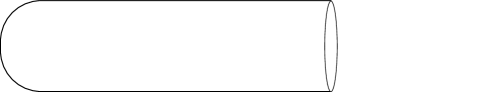
Figure 1.1. A cigar-shaped warped product.

Then for $r(t)>0$ all $g_{0}$-geodesics obey

$$\ddot{r}(t):=\frac{d^{2}}{dt^{2}}r(t)=2|\eta|^{2}F^{\prime}(r(t))F(r(t))^{-2}\geq 0,$$

where $r(t)$ is the $r$ coordinate of the geodesic at time $t$ and $\eta$ is the angular momentum. Consequently, the only trapped geodesics are the ones with $\dot{r}(t)\equiv F^{\prime}(r(t))\equiv 0$, that is the circular ones in the cylindrical end. This is the smallest amount of trapping a manifold with a cylindrical end can have.

Let $g$ be any metric such that $g-g_{0}$ is supported in $\{(r,\theta)\mid r<R\}$, and such that $g$ and $g_{0}$ have the same trapped geodesics. For example we may take $g=g_{0}+cg_{1}$, where $g_{1}$ is any symmetric two-tensor with support in $\{(r,\theta)\mid r<R\}$, and $c\in\mathbb{R}$ is chosen sufficiently small depending on $g_{1}$. Alternatively, we may take $g=dr^{2}+g_{S}(r)$, where $g_{S}(r)$ is a smooth family of metrics on the sphere such that $g_{S}(r)=r^{2}dS$ near $r=0$ and $g_{S}(r)=F(r)dS$ near $r\geq R$, and such that $\partial_{r}g_{S}(r)>0$ on $(0,R)$. This way we can construct examples where $g-g_{0}$ is not small.

Example 2.

Let $(X,g_{H})$ be a convex cocompact hyperbolic surface, such as the symmetric hyperbolic ‘pair of pants’ surface with three funnels depicted in Figure 1.2.

$r$ [l] at 280 -3 $\cosh^{2}\!r$ [l] at 225 70 $F(r)$ at 275 36                    

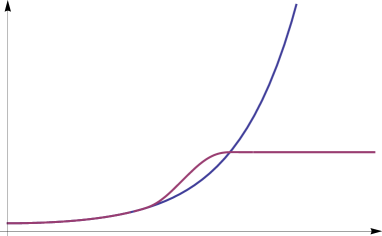
Figure 1.2. A hyperbolic surface $(X,g_{H})$ with three funnels, and a modification of the metric which changes the funnel ends to cylindrical ends.

In particular, there is a compact set $N\subset X$ (the convex core of $X$) such that

$$X\setminus N=(0,\infty)_{r}\times Y_{y},\qquad g_{H}|_{X\setminus N}=dr^{2}+\cosh^{2}\!r\,dy^{2},$$

where $Y$ is a disjoint union of $k\geq 1$ geodesic circles (possibly having different lengths).

We modify the metric in the funnel ends so as to change them into cylindrical ends in the following way. Take $g$ such that

$$g|_{N}=g_{H}|_{N},\qquad g|_{X\setminus N}=dr^{2}+F(r)dy^{2},$$

where $F(r)=\cosh^{2}\!r$ near $r=0$, and $F^{\prime}$ is compactly supported and positive on the interior of the convex hull of its support.

To obtain higher dimensional examples, we can take $(X,g_{H})$ to be a conformally compact manifold of constant negative curvature, with dimension $d\geq 3$, but in this case we need the additional assumption that the dimension of the limit set is less than $(d-1)/2$. The construction of $g$ now becomes more complicated and we give it in §3.3 below.

Our first result concerns only the above examples.

Theorem 1.1.

Let $(X,g)$ be as in Example 1 or 2 above, and let $\Delta\leq 0$ be its Laplacian. There is $z_{0}>0$ such that for any $\chi\in C_{c}^{\infty}(X)$ there is $C>0$ such that

$$\|\chi(-\Delta-z)^{-1}\chi\|_{L^{2}(X)\to L^{2}(X)}\leq C,$$ (1.1)

for all $z\in\mathbb{C}$ with $\operatorname{Re}z\geq z_{0}$ and $\operatorname{Im}z\neq 0$.

Here $(-\Delta-z)^{-1}$ denotes the standard resolvent which maps $L^{2}(X)\to L^{2}(X)$, and not its meromorphic continuation. Below, in Theorem 5.6, we also obtain bounds for the meromorphic continuation, but these are more complicated to state.

The bound (1.1) is optimal in the sense that we cannot replace the right hand side by a function of $z$ which tends to $0$ as $\operatorname{Re}z\to\infty$. Indeed, taking the case of Example 1 with $d=2$ for definiteness, we have $(-\Delta-k^{2})v(r)e^{ik\theta}=-v^{\prime\prime}(r)e^{ik\theta}$ for any $v\in C_{c}^{\infty}((R,\infty))$ and $k\in\mathbb{Z}$.

Note also that the resolvent in these examples is better behaved than it is for the (geometrically simpler) Riemannian product $(X,g)=(\mathbb{R}\times Y,g=dr^{2}+g_{Y})$, where $(Y,g_{Y})$ is a compact Riemannian manifold. Indeed, take $\chi\in C_{c}^{\infty}(X)$ a function of $r$ such that $\chi\geq 0$ and $\chi\not\equiv 0$, and take $\chi_{0}\in C_{c}^{\infty}(X)$ such that $\chi_{0}\chi=\chi$, and let $\phi$ be an eigenfunction of the Laplacian on $(Y,g_{Y})$ with $-\Delta\phi=\sigma^{2}\phi$. Then, by separation of variables,

$$\begin{split}\|\chi(-\Delta-z)^{-1}\chi\chi_{0}\phi\|_{L^{2}(X)}&=\|\phi\|_{L^{2}(Y)}\|\chi(-\partial_{r}^{2}-z+\sigma^{2})^{-1}\chi\|_{L^{2}(\mathbb{R})}\xrightarrow{z\to\sigma^{2}}+\infty,\end{split}$$ (1.2)

where we take the limit using the explicit formula for the resolvent [DyZw, (2.2.1)]. For our proof of Theorem 1.1 it will be crucial that $F^{\prime}>0$ near the cylindrical ends in Examples 1 and 2, and this is what is missing in the Riemannian product just discussed.

We will deduce Theorem 1.1 from Theorem 3.1 below, which gives a stronger result (allowing $\chi$ to be replaced by a noncompactly supported weight) and also applies to Schrödinger operators on more general manifolds with asymptotically cylindrical ends. We will further prove in Theorem 3.2 that we can obtain stronger resolvent bounds by suitably refining the cutoffs $\chi$.

An estimate like (1.1) has well-known implications for the spectrum of $-\Delta$. In particular, by [ReSi, Theorem XIII.20], the spectrum is purely absolutely continuous on $(z_{0},\infty)$, which rules out any embedded eigenvalues there, and we will see below, in §5, that embedded resonances (resonances on the real line, embedded in the continuous spectrum) are also ruled out.

To our knowledge ours is the first result ruling out the presence of infinitely many embedded eigenvalues or resonances for a large class of examples of manifolds with infinite cylindrical ends.

The situation can be very different for other manifolds with cylindrical ends. For example, let $X=\mathbb{R}\times Y$ and $g=dr^{2}+F(r)g_{Y}$, where $(Y,g_{Y})$ is a compact Riemannian manifold and $F\in C^{\infty}(\mathbb{R};(0,\infty))$, $1-F$ is compactly supported, and $\max F>1$. Then $-\Delta$ has infinitely many embedded eigenvalues converging to $+\infty$ ([ChZw, §3], [Pa2, (3.6)]).

The study of the spectral and scattering theory of the Laplacian on manifolds with cylindrical ends, and their perturbations, goes back to Guillopé [Gu] and Melrose [Me] and is an active and wide-ranging area of research: see for example [IsKuLa, MüSt, RiTi] for some recent results and more references. There is also a large of body of literature on the closely related study of the Laplacian on waveguides: something of a survey can be found in [KrKř], and let us also mention the older result [Go], and that there is a nonexistence result for eigenvalues in [DaPa]. In a slightly different direction, weighted resolvent estimates up to the spectrum and limiting absorption principles have been investigated using Mourre theory [Mo, AmBoGe, DeGé], and this has been applied to geometric situations such as ours in [Ni].

Our results also have implications for the distribution of resonances; these are the poles of the meromorphic continuation of the resolvent, and their study in this context also goes back to [Gu, Me]. An existence result for resolvent poles (in the presence of appropriate quasimodes, and which may be embedded in the real line or complex) on waveguides can be found in [Ed], and for more such results see [KrKř]. Upper bounds on the number resonances for manifolds with infinite cylindrical ends are given in [Ch1].

In Theorem 5.6, we will use an identity due to Vodev [Vo] to prove that (1.1) (or a more general resolvent estimate up to the spectrum) implies the existence of a resonance free region near the continuous spectrum. In a companion paper to this one, [ChDa1], we use these results to prove an asymptotic expansion for solutions to the wave equation.

1.2. Repulsive potentials on the half line

In this paper we also obtain some resolvent estimates for Schrödinger operators on the half line which we need in the course of the proofs of our main results, and which may be of independent interest. We state them here.

Let $V_{D}$ be a bounded, nonnegative, nonincreasing potential on the half line, such that

$$V_{D}^{\prime}(r)\leq-\delta_{V}(1+r)^{-1}V_{D}(r)\leq 0,$$ (1.3)

for some $\delta_{V}>0$ and for all $r\geq 0$, where if $V_{D}$ is not everywhere differentiable then (1.3) is meant in the sense of measures. Note that in particular the potential is repulsive in the sense of classical mechanics, since $V_{D}^{\prime}(r)<0$ except where $V_{D}(r)=0$.

For $h>0$ and $\zeta\in\mathbb{C}\setminus[0,\infty)$ let

$$(-h^{2}\partial_{r}^{2}+V_{D}-\zeta)^{-1}$$

denote the Dirichlet resolvent. In this paper we prove the following semiclassical resolvent estimates:

Theorem 1.2.

For all $s,\ s_{1},\ s_{2}>1/2$ with $s_{1}+s_{2}>2$ there is $C>0$ such that for all $\zeta\in\mathbb{C}\setminus[0,\infty)$ and $h>0$ we have

$$\|(1+r)^{-s}(-h^{2}\partial_{r}^{2}+V_{D}(r)-\zeta)^{-1}(1+r)^{-s}\|\leq\frac{C}{h\sqrt{|\zeta|}},$$ (1.4)

$$\|(1+r)^{-s_{1}}(-h^{2}\partial_{r}^{2}+V_{D}(r)-\zeta)^{-1}(1+r)^{-s_{2}}\|\leq\frac{C}{h^{2}},$$ (1.5)

and

$$\|V_{D}(r)^{1/2}(1+r)^{-1/2}(-h^{2}\partial_{r}^{2}+V_{D}(r)-\zeta)^{-1}(1+r)^{-s}\|\leq\frac{C}{h},$$ (1.6)

where the norms are $L^{2}(\mathbb{R}_{+})\to L^{2}(\mathbb{R}_{+})$.

Recall that, in the case $V_{D}\equiv 0$, (1.4) and (1.5) are well known to be sharp as dist$(\zeta,[0,\infty))\to 0$; this can be checked from the explicit formula for the resolvent in that case, which we give below in (5.4).

In fact, we will deduce these estimates from some uniform estimates for Schrödinger operators with repulsive potentials, replacing $C$ by an explicit constant. To state them, let

$$P_{D}:=-\partial_{r}^{2}+V_{D}(r),$$

regarded as a self-adjoint operator on $L^{2}(\mathbb{R}_{+})$ with domain $\{u\in H^{2}(\mathbb{R}_{+})\mid u(0)=0\}$.

Theorem 1.3.

For all $\delta>0$, $\theta\in[0,1]$, and $z\in\mathbb{C}\setminus[0,\infty)$, we have

$$\|(1+r)^{-\frac{1+\delta}{2}}(P_{D}-z)^{-1}(1+r)^{-\frac{1+\delta}{2}}\|\leq\frac{1+\sqrt{2}}{\sqrt{|z|}}\left(\frac{1}{\delta}+\frac{1}{\delta_{V}}\right),$$ (1.7)

$$\|(1+r)^{-\frac{1+\delta}{2}-\theta}(P_{D}-z)^{-1}(1+r)^{-\frac{1+\delta}{2}-(1-\theta)}\|\leq(1+\sqrt{2})\left(\frac{1}{\delta}+\frac{1}{\delta_{V}}\right),$$ (1.8)

and

$$\|V_{D}(r)^{\frac{\theta}{2}}(1+r)^{-\frac{1+(1-\theta)\delta}{2}}(P_{D}-z)^{-1}V_{D}(r)^{\frac{1-\theta}{2}}(1+r)^{-\frac{1+\theta\delta}{2}}\|\leq\frac{2\sqrt{2}}{\delta_{V}}\sqrt{1+\frac{\delta_{V}}{\delta}},$$ (1.9)

where the norms are $L^{2}(\mathbb{R}_{+})\to L^{2}(\mathbb{R}_{+})$.

Note that Theorem 1.3 implies Theorem 1.2.

If $V_{D}\in C^{1}([0,\infty))$ is compactly supported and has $V_{D}^{\prime}<0$ on the interior of the support of $V_{D}$, then (1.3) is satisfied for some $\delta_{V}>0$ (because $\log V_{D}$ and $(\log V_{D})^{\prime}$ tend to $-\infty$ at the boundary of the support). Moreover the class of potentials satisfying (1.3) for a given $\delta_{V}>0$ is closed under nonnegative linear combinations and contains all functions of the form $(1+r)^{-m}$ with $m\geq\delta_{V}$. The same proof could also handle potentials $V_{D}$ satisfying (1.3) and such that $V_{D}(r)\to\infty$ as $r\to 0$, provided $V_{D}(r)|u(r)|^{2}\to 0$ as $r\to 0$ for all $u$ in the domain of $P_{D}$.

The bounds (1.4) and (1.7) are best when the spectral parameter is not too close to $0$, and (1.5) and (1.8) are best when the spectral parameter is close to $0$. We can think of (1.6) and (1.9) as being a kind of Agmon or elliptic estimate in the limit $|z|\to 0$ (see also (4.14) below); they give an improvement when we are looking at the resolvent in the elliptic and classically forbidden range in the interior of the support of $V_{D}$. When $V_{D}(r)\sim(1+r)^{-m}$ as $r\to\infty$ for some $m>0$, the weights in (1.9) are also to be compared to the weights in [Ya, Na]; see in particular [Na, Theorem 1.3].

If we do not demand explicit constants in the estimates, then Theorem 1.3 is essentially well-known if either $V_{D}(0)$ (which we can think of as a coupling constant) is not large (see [Ya, Chapter 4] for a more general discussion of scattering on the half line, and [KoTr] for some more recent results and references), or if $V_{D}(0)$ and $|z|$ are large (this is the semiclassical, nontrapping regime: see [Ya, Chapter 7, Theorem 1.6] for a similar result). The main novelty here is that we cover all values of $V_{D}(0)$ and $|z|$ uniformly, and for our applications in §3 we will especially need the case where $V_{D}(0)$ is large compared to $|z|$: this corresponds to a low-energy semiclassical problem.

We prove Theorem 1.3 in §2 below.

1.3. Notation

Throughout the paper $C$ is a large constant which can change from line to line, and all estimates are uniform for $h\in(0,h_{1}]$, where $h_{1}$ can change from line to line. It will sometimes be convenient to write derivatives with respect to $r$ using the notation $D_{r}:=-i\partial_{r}$. We use

$$\|u\|_{H^{m}_{h}(X)}:=\|(-h^{2}\Delta+1)^{m/2}u\|_{L^{2}(X)},$$

and similarly define $\|u\|_{H^{m}_{h}(\mathbb{R})}$ and $\|u\|_{H^{m}_{h}(\mathbb{R}_{+})}$ (in the latter case we will only be concerned with $u$ vanishing near $r=0$, so the boundary condition on the Laplacian implicit in the notation in this case is immaterial).

The energy level $E_{0}>0$ is fixed in §3.1, along with the rest of the notation needed for our general abstract setup of a mildly trapping Schrödinger operator on a manifold with asymptotically cylindrical ends. The auxiliary notations $E_{j}$ and $E_{*}$ are defined in §4.2 in terms of this setup. The notation $E$ without a subscript is used in §2 and §5 to denote a variable positive energy, not related in any particular way to $E_{0}$ or $E_{j}$ or $E_{*}$.

The radial variable $r$ on the cylindrical end has the same meaning in §3.1, in §4, and in §5. The usage in §2 is consistent with this usage, if we separate variables to write Schrödinger operator on an asymptotically cylindrical end as a sum of Schrödinger operators on $\mathbb{R}_{+}$. For example, if $\Delta$ is the Laplacian on $((0,\infty)\times Y,dr^{2}+g_{Y})$ we write

$$-\Delta=\sum_{j=0}^{\infty}(-\partial_{r}^{2}+\sigma_{j}^{2})\phi_{j}\otimes\phi_{j},\text{ to mean }-\Delta u=\sum_{j=0}^{\infty}\phi_{j}\int_{Y}(-\partial_{r}^{2}+\sigma_{j}^{2})u(r,y)\phi_{j}(y)d\!\operatorname{vol}(y),$$

where $\{\phi_{j}\}_{j=0}^{\infty}$ is a complete set of real-valued orthonormal eigenfunctions of the Laplacian on $Y$ and $-\Delta_{Y}\phi_{j}=\sigma_{j}^{2}\phi_{j}$.

Of course the results of §2 also apply to more general Schrödinger operators on $\mathbb{R}_{+}$.

The variable $r$ is used a little differently in §1.1, §3.3, and §3.4. To convert the $r$ in one of these sections to the $r$ in the rest of the paper, use the affine map

$$r\mapsto 6(r-R_{1})/(R_{2}-R_{1}),$$ (1.10)

for suitably chosen $R_{1}$ and $R_{2}$, and then multiply $g$ by $(R_{2}-R_{1})^{2}/36$ to remove the factor that appears in front of $dr^{2}$. For Example 1, take $R_{1}$ such that $\inf\{r>0\mid g(r,y)=g_{0}(r,y)\textrm{ for all }y\}<R_{1}<R$ and use $R_{2}=R$. For Example 2, let $R_{2}=\max\operatorname{supp}F^{\prime}$, and take $R_{1}\in(0,R_{2})$. For §3.3, let $R_{1}=R+1$ and $R_{2}=\max\operatorname{supp}F^{\prime}$. For §3.4, let $R_{1}=R/2$ and $R_{2}=R$.

Contents

1. 1 Introduction
2. 2 Resolvent estimates on the half line
3. 3 Resolvent estimates for mildly trapping manifolds
4. 4 Proof of Theorems 3.1 and 3.2
5. 5 Continuation of the resolvent

2. Resolvent estimates on the half line

In this section we prove Theorem 1.3. All function norms and inner products in this section are in $L^{2}(\mathbb{R}_{+})$, and operator norms are $L^{2}(\mathbb{R}_{+})\to L^{2}(\mathbb{R}_{+})$.

Proof of (1.7).

Let $E:=\operatorname{Re}z$ and $\varepsilon:=|\operatorname{Im}z|$. We begin by proving an a priori estimate when $E>0$ and $\varepsilon>0$. Roughly speaking, the idea is to exploit the fact that, since $V_{D}^{\prime}\leq 0$, we have the positive commutator $[P_{D},r\partial_{r}]=-2\partial_{r}^{2}-rV_{D}^{\prime}(r)\geq 0$. However, to be able to control the remainder terms in our positive commutator argument, we must replace $r\partial_{r}$ with $w(r)\partial_{r}$ where $w$ grows more slowly. Such commutants have been used by many authors (see [ReSi, §XIII.7] and references therein); below we take an approach inspired by [Vo, Da1] and papers cited therein.

Take $w\in C^{1}([0,\infty);[0,1])$ such that $w^{\prime}(r)>0$ for all $r\geq 0$, and take $u\in H^{2}(\mathbb{R}_{+})$ such that $u(0)=0$ and $(w^{\prime})^{-1/2}(P_{D}-z)u\in L^{2}$; in particular, $u(r)$ and $u^{\prime}(r)$ tend to $0$ as $r\to\infty$. Adding together the integration by parts identities

$$-\langle(w(V_{D}-E))^{\prime}u,u\rangle=2\operatorname{Re}\langle w(V_{D}-E)u,u^{\prime}\rangle,$$

and

$$\langle w^{\prime}u^{\prime},u^{\prime}\rangle+w(0)|u^{\prime}(0)|^{2}=-2\operatorname{Re}\langle wu^{\prime\prime},u^{\prime}\rangle,$$

gives

$$\begin{split}E\|\sqrt{w^{\prime}}u\|^{2}+\|\sqrt{w^{\prime}}u^{\prime}\|^{2}-\langle(wV_{D})^{\prime}u,u\rangle&+w(0)|u^{\prime}(0)|^{2}=2\operatorname{Re}\langle w(P_{D}-z)u,u^{\prime}\rangle-2\operatorname{Im}z\operatorname{Im}\langle wu,u^{\prime}\rangle.\end{split}$$

Since $0\leq w\leq 1$, this implies

$$E\|\sqrt{w^{\prime}}u\|^{2}+\|\sqrt{w^{\prime}}u^{\prime}\|^{2}-\langle(wV_{D})^{\prime}u,u\rangle\leq 2\left\|\frac{1}{\sqrt{w^{\prime}}}(P_{D}-z)u\right\|\|\sqrt{w^{\prime}}u^{\prime}\|+2\varepsilon\|u\|\|u^{\prime}\|.$$ (2.1)

Later we will choose $w$ so that $(wV_{D})^{\prime}\leq 0$, but first we estimate the second term on the right, which we think of as a remainder term. Since $V_{D}\geq 0$, integrating by parts gives

$$\|u^{\prime}\|^{2}\leq\operatorname{Re}\langle(P_{D}-z)u,u\rangle+E\|u\|^{2}\leq\left\|\frac{1}{\sqrt{w^{\prime}}}(P_{D}-z)u\right\|\|\sqrt{w^{\prime}}u\|+E\|u\|^{2},$$

and we also have

$$\varepsilon\|u\|^{2}=|\operatorname{Im}\langle(P_{D}-z)u,u\rangle|\leq\left\|\frac{1}{\sqrt{w^{\prime}}}(P_{D}-z)u\right\|\|\sqrt{w^{\prime}}u\|.$$

Combining these gives

$$\varepsilon^{2}\|u\|^{2}\|u^{\prime}\|^{2}\leq(E+\varepsilon)\left\|\frac{1}{\sqrt{w^{\prime}}}(P_{D}-z)u\right\|^{2}\|\sqrt{w^{\prime}}u\|^{2},$$

and then plugging this into (2.1) gives

$$E\|\sqrt{w^{\prime}}u\|^{2}+\|\sqrt{w^{\prime}}u^{\prime}\|^{2}-\langle(wV_{D})^{\prime}u,u\rangle\leq 2\left\|\frac{1}{\sqrt{w^{\prime}}}(P_{D}-z)u\right\|\left(\|\sqrt{w^{\prime}}u^{\prime}\|+\sqrt{E+\varepsilon}\|\sqrt{w^{\prime}}u\|\right).$$

Completing the square gives

$$\begin{split}\left(\sqrt{E}\|\sqrt{w^{\prime}}u\|-\frac{\sqrt{E+\varepsilon}}{\sqrt{E}}\left\|\frac{1}{\sqrt{w^{\prime}}}(P_{D}-z)u\right\|\right)^{2}&+\left(\|\sqrt{w^{\prime}}u^{\prime}\|-\left\|\frac{1}{\sqrt{w^{\prime}}}(P_{D}-z)u\right\|\right)^{2}\\ -&\langle(wV_{D})^{\prime}u,u\rangle\leq\frac{2E+\varepsilon}{E}\left\|\frac{1}{\sqrt{w^{\prime}}}(P_{D}-z)u\right\|^{2}.\end{split}$$ (2.2)

We now take

$$w(r):=1-\frac{\delta_{V}}{\delta_{V}+\delta}(1+r)^{-\delta},$$ (2.3)

so that, by (1.3), we have

$$(wV_{D})^{\prime}(r)=\frac{\delta\delta_{V}V_{D}(r)}{(\delta_{V}+\delta)(1+r)^{1+\delta}}+w(r)V_{D}^{\prime}(r)\leq\frac{\delta_{V}V_{D}(r)}{1+r}\left((1+r)^{-\delta}-1\right)\leq 0,$$ (2.4)

where, as with (1.3), we understand (2.4) in the sense of measures in the case that $V_{D}$ is not differentiable everywhere. We may now drop the second and third terms from the left hand side of (2.2), giving

$$\sqrt{E}\|\sqrt{w^{\prime}}u\|\leq\frac{\sqrt{E+\varepsilon}+\sqrt{2E+\varepsilon}}{\sqrt{E}}\left\|\frac{1}{\sqrt{w^{\prime}}}(P_{D}-z)u\right\|.$$ (2.5)

From (2.5) we can deduce a weighted resolvent estimate when $\operatorname{Re}z>0$, $\operatorname{Im}z\neq 0$. To obtain an estimate for all $z\in\mathbb{C}\setminus[0,\infty)$, we use the Phragmén–Lindelöf principle in the following way. For $u,\ v\in L^{2}(\mathbb{R}_{+})$, put

$$U(z):=\langle(1+r)^{-\frac{1+\delta}{2}}(P_{D}-z)^{-1}(1+r)^{-\frac{1+\delta}{2}}u,v\rangle\sqrt{z},$$ (2.6)

and for $\alpha>0$ put

$$\Omega_{\alpha}:=\{z\in\mathbb{C}\mid\alpha\operatorname{Re}z<|\operatorname{Im}z|\}.$$

Then $U$ is holomorphic in $\Omega_{\alpha}$, where it obeys

$$|U(z)|\leq\frac{|\sqrt{z}|\|u\|\|v\|}{\textrm{dist}(z,[0,\infty))}\leq\frac{\sqrt{1+\alpha^{-2}}\|u\|\|v\|}{|\sqrt{z}|}$$

Moreover, by (2.5), for $z\in\partial\Omega_{\alpha}\setminus\{0\}$, we have

$$|U(z)|\leq\left(\sqrt{1+\alpha}+\sqrt{2+\alpha}\right)\left(\delta^{-1}+\delta_{V}^{-1}\right)\|u\|\|v\|.$$ (2.7)

Then the Phragmén–Lindelöf principle (see e.g. [ReSi, p. 236]) implies (2.7) for all $z\in\Omega_{\alpha}$. Taking $\alpha\to 0$ gives (1.7). ∎

Proof of (1.8).

We begin by following the proof of (1.7), but we drop the first term, rather than the second, from the left hand side of (2.2), so that in place of (2.5) we have

$$\|\sqrt{w^{\prime}}u^{\prime}\|\leq\left(1+\sqrt{2+\varepsilon E^{-1}}\right)\left\|\frac{1}{\sqrt{w^{\prime}}}(P_{D}-z)u\right\|.$$

We now integrate by parts to obtain a weighted version of the Poincaré inequality:

$$\left\|(1+r)^{\frac{-3-\delta}{2}}u\right\|^{2}=\frac{2}{2+\delta}\operatorname{Re}\left\langle(1+r)^{-2-\delta}u^{\prime},u\right\rangle\leq\left\|(1+r)^{\frac{-1-\delta}{2}}u^{\prime}\right\|\left\|(1+r)^{\frac{-3-\delta}{2}}u\right\|,$$

giving

$$\left\|(1+r)^{\frac{-3-\delta}{2}}u\right\|\leq\sqrt{\delta_{V}^{-1}+\delta^{-1}}\left(1+\sqrt{2+\varepsilon E^{-1}}\right)\left\|\frac{1}{\sqrt{w^{\prime}}}(P_{D}-z)u\right\|.$$ (2.8)

We now apply the Phragmén–Lindelöf principle as in the proof of (1.7), with the difference that in place of (2.6) we use

$$U(z):=\langle(1+r)^{-\frac{3+\delta}{2}}(P_{D}-z)^{-1}(1+r)^{-\frac{1+\delta}{2}}u,v\rangle,$$

to obtain (1.8) when $\theta=1$. Then taking the adjoint gives the result for $\theta=0$, and interpolating (that is to say, applying the Phragmén–Lindelöf principle with respect to $\theta\in\mathbb{C}$ such that $\operatorname{Re}\theta\in[0,1]$) gives the result for $\theta\in(0,1)$. ∎

Proof of (1.9).

We again proceed as in the proof of (1.7), but this time we replace (2.3) by

$$w(r):=1-\frac{\delta_{V}}{2(\delta_{V}+\delta)}(1+r)^{-\delta},$$

so that (2.4) is replaced by

$$(wV_{D})^{\prime}(r)\leq-\frac{\delta_{V}V_{D}(r)}{2(1+r)}.$$

Now dropping the first two terms on the left hand side of (2.2) gives

$$\left\langle\frac{\delta_{V}V_{D}(r)}{2(1+r)}u,u\right\rangle\leq\frac{2E+\varepsilon}{E}\left\|\frac{1}{\sqrt{w^{\prime}}}(P_{D}-z)u\right\|^{2},$$

or

$$\|V_{D}(r)^{\frac{1}{2}}(1+r)^{-\frac{1}{2}}(P_{D}-z)^{-1}(1+r)^{-\frac{1+\delta}{2}}\|\leq\frac{2\sqrt{2+\varepsilon E^{-1}}}{\sqrt{\delta_{V}}}\sqrt{\delta^{-1}+\delta_{V}^{-1}}.$$

We now proceed as in the proof of (1.8), applying the Phragmen–Lindelöf principle to obtain (1.9) for $\theta=1$, and then taking the adjoint and interpolating to obtain (1.9) for $\theta\in[0,1)$. ∎

3. Resolvent estimates for mildly trapping manifolds

In §3.1 we state our main resolvent estimates for mildly trapping manifolds with asymptotically cylindrical ends, under suitable abstract assumptions. In the remainder of §3 we give examples which satisfy the assumptions, and then in §4 we prove the estimates.

3.1. Resolvent estimates for asymptotically cylindrical manifolds

Let $(X,g)$ be a smooth Riemannian manifold of dimension $d\geq 2$, with or without boundary, with the following kind of asymptotically cylindrical ends: we assume there is an open set $X_{e}\subset X$ such that $\partial X\cap X_{e}=\varnothing$, $X\setminus X_{e}$ is compact, and

$$X_{e}=(0,\infty)_{r}\times Y,\qquad g|_{X_{e}}=dr^{2}+f(r)^{4/(d-1)}g_{Y}.$$

Here $Y$ is a compact, not necessarily connected, manifold without boundary of dimension $d-1$, $g_{Y}$ is a fixed smooth metric on $Y$ and $f\in C^{\infty}([0,\infty);(0,1])$. We suppose further that there is $\delta_{0}>0$ such that

$$|(f-1)^{(k)}(r)|\leq C_{k}(1+r)^{-k-\delta_{0}}\textrm{ for all }k\in\mathbb{N}_{0}\textrm{ and }r\geq 0,$$ (3.1)

and

$$f^{\prime}(r)\geq\delta_{0}(1+r)^{-1}(1-f)\geq 0\textrm{ for all }r\geq 0.$$ (3.2)

Suppose finally that $f(r)<1$ for $r<6$. Note that if we replace $r<6$ by $r<r_{0}$ in this last condition, we can reduce to the case $r_{0}=6$ by multiplying $g$ by a constant and rescaling $r$ (i.e. using (1.10) with $R_{1}=0$ and $R_{2}=r_{0}$).

We briefly discuss the assumptions (3.1) and (3.2). Note that the class of functions $f$ such that (3.1) and (3.2) hold for a given $\delta_{0}>0$ is convex, and contains all functions of the form $f(r)=1-(1+r)^{-m}$ whenever $m\geq\delta_{0}$. Moreover, all functions $f$, such that $f^{\prime}$ is compactly supported and positive on the interior of the support of $(1-f)$, obey (3.1) and (3.2) for some $\delta_{0}>0$; indeed, letting $R_{f}:=\max\operatorname{supp}(1-f)$, we have

$$\lim_{r\uparrow R_{f}}\log(1-f(r))=\lim_{r\uparrow R_{f}}\frac{d}{dr}\log(1-f(r))=-\infty.$$

If $f^{\prime}$ is compactly supported then the ends are cylindrical, rather than just asymptotically cylindrical.

For notational convenience let us extend $r$ to be a continuous function on $X$ with $-1/2\leq r<0$ on $X\setminus\overline{X_{e}}$, and extend $f$ to be constant for $r\leq 0$.

Let $\Delta\leq 0$ be the Laplacian on $X$. Let

$$P=P_{h}:=-h^{2}\Delta+V,$$

where $h\in(0,h_{0}]$ for some $h_{0}>0$, and:

• $V=V_{h}\in C^{\infty}(X\times(0,h_{0}];\mathbb{R})$ is bounded, together with all derivatives, uniformly in $h\in(0,h_{0}]$.

• $V|_{X_{e}}$ is a function of $r$ and $h$ only, and has a decomposition $V|_{X_{e}}=V_{L}+hV_{S}$, where $V_{L}$ and $V_{S}$ may also depend on $h$, and $V_{S}=0$ for $r\geq 5$ and $|V_{S}^{(k)}(r)|+|V_{L}^{(k)}(r)|\leq C_{k}(1+r)^{-k-\delta_{0}}$ for all $k\geq 0$, uniformly in $h$.

• $V_{L}^{\prime}(r)\leq-\delta_{0}(1+r)^{-1}V_{L}(r)\leq 0$ for all $r\geq 0$.

Note that the assumptions allow $V\equiv 0$ but not $f\equiv 1$. Such a restriction is necessary to obtain a resolvent bound which is uniform up to the spectrum, in light of the computation in (1.2), which rules out such a bound in the case $(X,g)=(\mathbb{R}\times Y,dr^{2}+dS)$ and $P=-h^{2}\Delta$.

Fix $E_{0}>0$. We suppose that $E_{0}$ is a “mildly trapping” energy level for $P$ in the sense that adding a complex absorbing barrier supported on $X_{e}$ gives a polynomial resolvent bound. More specifically, suppose that for some $W_{K}\in C^{\infty}(\mathbb{R};[0,1])$ with $W_{K}=0$ near $(-\infty,5]$ and $W_{K}=1$ near $[6,\infty)$, there is $N\in\mathbb{R}$ such that

$$\|(P-iW_{K}(r)-E_{0})^{-1}\|_{L^{2}(X)\to L^{2}(X)}=:a(h)h^{-1}\leq h^{-N},$$ (3.3)

for all $h\in(0,h_{0}]$.

We have the following weighted resolvent bound up to the spectrum.

Theorem 3.1.

Let $(X,g),\ P,\ E_{0},$ and $a(h)$ be as above. Fix $s_{1},\ s_{2}>1/2$ such that $s_{1}+s_{2}>2$. There are $C>0$ and $h_{1}>0$ such that

$$\|(1+r)^{-s_{1}}(P-E_{0}-i\varepsilon)^{-1}(1+r)^{-s_{2}}\|_{L^{2}(X)\to L^{2}(X)}\leq C(a(h)+h^{-1})h^{-1},$$ (3.4)

for all $\varepsilon\in\mathbb{R}\setminus 0$ and for all $h\in(0,h_{1}]$.

Note that the condition on $s_{1}$ and $s_{2}$ is the same as the one in §1.2 above, see in particular (1.5) and (1.8). This is the resolvent weighting needed to have a low energy bound for scattering on the half line (and for more general Euclidean scattering problems).

To deduce Theorem 1.1 from Theorem 3.1, in Examples 1 and 2 we let $X_{e}$ be the part of $X$ where $r\geq r_{1}$, for any $r_{1}>0$ such that $F^{\prime}(r_{1})>0$, and put $V\equiv 0$. Then, after redefining $r$ as in the remark following (3.2), we see that $g$ has the desired form in $X_{e}$, and it remains to check that (3.3) holds with $N\leq 2$. Below in §3.2 and §3.3 we will show this for some examples which generalize Examples 1 and 2 above.

We also have an improved bound when we cut off away from the trapping in the end. To state it, let $\chi_{\Pi}\in C^{\infty}(\mathbb{R};[0,1])$ be $0$ near $(-\infty,0]$ and $1$ near $[1,\infty)$. Let $\Delta_{Y}\leq 0$ be the Laplacian on $(Y,g_{Y})$, and let $\{\phi_{j}\}_{j=0}^{\infty}$ be a complete real-valued orthonormal set of its eigenfunctions, with $-\Delta_{Y}\phi_{j}=\sigma_{j}^{2}\phi_{j}$, where $0=\sigma_{0}\leq\sigma_{1}\leq\cdots$. For any $\mathcal{J}\subset\{0,\ 1,\ \dots\}$, we denote the orthogonal projection onto modes corresponding to $\mathcal{J}$ by $\Pi_{\mathcal{J}}\colon L^{2}(X_{e})\to L^{2}(X_{e})$, so that

$$(\Pi_{\mathcal{J}}u)(r,y):=\sum_{j\in\mathcal{J}}\phi_{j}(y)\int_{Y}u(r,y^{\prime})\phi_{j}(y^{\prime})d\!\operatorname{vol}(y^{\prime}),$$

where $y$ and $y^{\prime}$ denote points in $Y$. Then $\|\Pi_{\mathcal{J}}\chi_{\Pi}(r)\|_{L^{2}(X)\to L^{2}(X)}=1$, unless $\mathcal{J}$ is empty.

Theorem 3.2.

Fix $s>1/2$ and $c_{\mathcal{J}}>0$. Let $\mathcal{J}:=\{j\mid E_{j}:=E_{0}-h^{2}\sigma_{j}^{2}\not\in[-c_{\mathcal{J}}h,c_{\mathcal{J}}]\}$. Define a microlocal cutoff $\chi_{\mathcal{J}}\colon L^{2}(X)\to L^{2}(X)$ by putting

$$\chi_{\mathcal{J}}u:=\begin{cases}\left(\Pi_{\mathcal{J}}\chi_{\Pi}(r)+\sqrt{V_{L}(r)+f(r)^{-4/(d-1)}-1}\right)u,\quad&u\in L^{2}(X_{e}),\\ u,\quad&u\in L^{2}(X\setminus X_{e}),\end{cases}$$ (3.5)

and then extending to general $u\in L^{2}(X)$ by linearity. There are $C>0$ and $h_{1}>0$ such that

$$\|(1+r)^{-s}\chi_{\mathcal{J}}(P-E_{0}-i\varepsilon)^{-1}(1+r)^{-s}\|_{L^{2}(X)\to L^{2}(X)}\leq C(1+a(h))h^{-1},$$ (3.6)

for all $\varepsilon\in\mathbb{R}\setminus 0$ and for all $h\in(0,h_{1}]$.

By taking the adjoint, we see that (3.6) implies

$$\|(1+r)^{-s}(P-E_{0}-i\varepsilon)^{-1}\chi_{\mathcal{J}}(1+r)^{-s}\|_{L^{2}(X)\to L^{2}(X)}\leq C(1+a(h))h^{-1}.$$ (3.7)

Note that the statement is strongest when $c_{\mathcal{J}}$ is chosen very small, much smaller than $E_{0}$. We think of $\chi_{\mathcal{J}}$ as cutting off away from (or, almost, projecting away from)

$$T_{\mathcal{J}}=\{u\in L^{2}(X_{e})\mid fu=u,\ V_{L}u=0,\ \Pi_{\mathcal{J}}u=0\}\subset L^{2}(X).$$

Observe that the condition $E_{j}\in[-c_{\mathcal{J}}h,c_{\mathcal{J}}]$ corresponds, when $V_{L}=0$ and $f=1$, to the condition that $\rho^{2}\in[-c_{\mathcal{J}}h,c_{\mathcal{J}}]$, where $\rho$ is the dual variable to $r$. In this sense $T_{\mathcal{J}}$ corresponds to a neighborhood of the bicharacteristics in $T^{*}X_{e}$ along which $r$ is constant, that is to say bicharacteristics trapped in the cylindrical ends. In this sense $\chi_{\mathcal{J}}$ cuts off away from the trapping in the cylindrical ends. The asymmetry in the interval $[-c_{\mathcal{J}}h,c_{\mathcal{J}}]$ is due to the fact that our estimates are much easier when $E_{j}\leq-Ch$ for any $C>0$ (see in particular the sentence following (4.41) below); we do not expect this form of the interval to be optimal.

To simplify matters, in our discussion of the interpretation and context of this result we focus on the special case of the following Corollary, although most of the statements could be adapted to apply to the more general case.

Corollary 3.3.

Let $(X,g)=(\mathbb{R}^{d},g)$ be as in Example 1. In the notation of that example, fix $\chi\in C_{c}^{\infty}(X)$ with $\operatorname{supp}\chi\subset\{(r,\theta)\in\mathbb{R}^{d}\mid r<R\}$, and fix $s>1/2$. Then there are $z_{0}>0$ and $C>0$ such that

$$\|(1+r)^{-s}(-\Delta-z)^{-1}\chi\|_{L^{2}(X)\to L^{2}(X)}+\|\chi(-\Delta-z)^{-1}(1+r)^{-s}\|_{L^{2}(X)\to L^{2}(X)}\leq C/\sqrt{\operatorname{Re}z},$$ (3.8)

for all $z\in\mathbb{C}$ with $\operatorname{Re}z\geq z_{0}$ and $\operatorname{Im}z\neq 0$.

Note that this $\chi$ is local, in contrast to the microlocal $\chi_{\mathcal{J}}$ of Theorem 3.2. Recall that $R$ is the radius at which the cylindrical end begins; hence $\chi$ is a cut off away from the trapping on the cylindrical end, and in this example there is no other trapping. The right hand side of (3.8) is the usual nontrapping upper bound, cf. (1.7) and the bound of $Ch^{-1}$ in (1.4). There have been many results in asymptotically Euclidean, conic, and hyperbolic scattering proving that such nontrapping bounds hold when one cuts off away from trapping on both sides of the resolvent: these go back to work of Cardoso and Vodev [CaVo], refining an earlier result of Burq [Bu1]. Intriguingly, in (3.8) we get a nontrapping bound by applying a spatial cutoff away from trapping on only one side of the resolvent; to our knowledge no such result is known in asymptotically Euclidean, conic, and hyperbolic scattering, although a related weaker bound can be found in [BuZw, Ch2, DaVa2] (and note that the weaker bound is shown to be optimal in a special example in [Dy]). A possible interpretation is the following: unlike in any of the examples studied in [BuZw, DaVa2], in Example 1 the set $K$ of bicharacteristics trapped as $t\to+\infty$ and $t\to-\infty$ is the same as the set $\Gamma_{\pm}$ of bicharacteristics trapped as $t\to+\infty$ or $t\to-\infty$, and one expects resolvent estimate losses due to mild trapping to be concentrated on $\Gamma_{\pm}$.

On the other hand, in [DaDyZw] it is shown that for a “well in an island” semiclassical Schrödinger operator (in which case incidentally $K$ does equal $\Gamma_{\pm}$), losses due to trapping extend beyond $\Gamma_{\pm}$ and cutting off on one side only is not enough to give nontrapping bounds; as discussed in that paper, this is closely related to the fact that the trapping in this case is stable (so that tunneling can produce losses away from $\Gamma_{\pm}$), unlike in Example 1 or in the examples in [DaVa2]. It is then natural to ask: when is cutting off a resolvent away from trapping on one side sufficient to give nontrapping bounds, and when is it necessary to cut off on both sides?

3.2. Examples with no trapping away from the ends

Let $X$ have no boundary and let $K_{E_{0}}$ be the set of bicharacteristics of $P$ at energy $E_{0}$ which do not intersect $T^{*}X_{e}$. If $K_{E_{0}}=\varnothing$, then it is essentially well-known that

$$\|(P-iW_{K}(r)-E_{0})^{-1}\|_{L^{2}(X)\to L^{2}(X)}\leq Ch^{-1};$$ (3.9)

the proof of (3.9) follows from the proof of [DyZw, Theorem 6.11] or that of [Da2, Proposition 3.2]. In the case that $|V|\leq Ch$, demanding that $K_{E_{0}}=\varnothing$ is equivalent to demanding that all maximally extended geodesics on $X$ intersect $X_{e}$; specific examples are given in Example 1.

3.3. Hyperbolic and normally hyperbolic trapped sets.

If $K_{E_{0}}\neq\varnothing$ we cannot hope to have (3.9), but if $K_{E_{0}}$ is hyperbolic or normally hyperbolic then we may have

$$\|(P-iW_{K}(r)-E_{0})^{-1}\|_{L^{2}(X)\to L^{2}(X)}\leq C\log(h^{-1})h^{-1}.$$ (3.10)

In the case of a closed hyperbolic orbit, such bounds are due to Burq [Bu2] and Christianson [Ch2]. For hyperbolic trapped sets satisfying a pressure condition they are due to Nonnenmacher and Zworski [NoZw1], and for normally hyperbolic trapped sets to Wunsch and Zworski [WuZw] and to Nonnenmacher and Zworski [NoZw2] (and see also [Dy]). Some recent surveys of the substantial wider literature concerning estimates like (3.10) can be found in [No, Zw2].

To deduce (3.10) from [NoZw1] or [NoZw2], note that the difference between (3.10) and [NoZw1, (2.7)] or [NoZw2, (1.18)] lies in the assumptions in the region where $W_{K}=1$. But in this region $P-iW_{K}$ is semiclassically elliptic, so the discrepancy can be removed using a parametrix $G^{\prime}$ analogous to the one in (4.1) below, and rather than having to go through a procedure like that in §4.5 we just have $(P-iW_{K}(r)-E_{0})G^{\prime}=I+O(h^{\infty})$.

Rather than discussing the general dynamical assumptions further, we now specialize to more concrete examples.

Let $(X,g_{H})$ be a conformally compact manifold of constant negative curvature. We recall that this means that the metric $g_{H}$ is asymptotically hyperbolic in the sense of [MaMe] (see also [DyZw, §5.1]), so there is an open set $X_{e}^{\prime}$ and $R\in\mathbb{R}$ such that $X\setminus X_{e}^{\prime}$ is compact and

$$X_{e}^{\prime}=(R,\infty)_{r}\times Y,\qquad g_{H}|_{X_{e}^{\prime}}=d{r}^{2}+e^{2r}g_{Y}(e^{-r}),$$

where $Y$ is a compact, not necessarily connected, manifold without boundary and $g_{Y}(x)$ is a family of metrics on $Y$ depending smoothly on $x$ up to $x=0$. Such a ‘normal form’ of the metric was first found in [GrLe], and it is also in [DyZw, §5.1.1].

We modify the metric to obtain a manifold with cylindrical ends in the following way. We first observe that, denoting points in $T^{*}X_{e}^{\prime}$ by $(r,y,\rho,\eta)$, where $y\in Y$, $\rho$ is dual to $r$, and $\eta$ is dual to $y$, along $g_{H}$-geodesics we have

$$\frac{d^{2}}{dt^{2}}r=:\ddot{r}=-2\partial_{r}(e^{-2r}|\eta|^{2}_{r,y})=4e^{-2r}|\eta|^{2}_{r,y}(1+O(e^{-r})),$$

where the length $|\eta|_{r,y}$ is taken with respect to the dual metric to $g_{Y}(e^{-r})$. Hence, after possibly redefining $R$ to be larger, we may suppose that $\ddot{r}\geq 2e^{-2r}|\eta|^{2}_{r,y}$ for $r\geq R$, and in particular that no bounded $g_{H}$-geodesics intersect $\overline{X_{e}^{\prime}}$. Indeed, since $E_{0}:=\rho^{2}+e^{-2r}|\eta|^{2}_{r,y}$ is conserved and $\dot{r}=2\rho$, in $X_{e}^{\prime}$ we have

$$\ddot{r}\geq 2e^{-2r}|\eta|^{2}_{r,y}=2E_{0}-\dot{r}^{2}/2,$$

which means $r$ is not bounded for all $t$.

Fix $\chi_{H}\in C^{\infty}(\mathbb{R};[0,1])$ such that $\chi_{H}(r)=1$ near $(-\infty,R]$ and $\chi_{H}(r)=0$ near $[R+1,\infty)$, and fix $F\in C^{\infty}([R,\infty),(0,\infty))$ such that $F^{\prime}$ is compactly supported, positive on the interior of its support, and such that $F^{\prime}(r)>0$ for $r\leq R+2$. Take $g$ such that $g|_{X\setminus X_{e}^{\prime}}=g_{H}|_{X\setminus X_{e}^{\prime}}$, and

$$g|_{X_{e}^{\prime}}=\chi_{H}(r)g_{H}+C_{g}(1-\chi_{H}(r))\left(dr^{2}+F(r)g_{Y}(0)\right).$$

We claim that if $C_{g}$ is large enough, then $\ddot{r}\geq 0$ along $g$-geodesics in $\overline{X_{e}}$. Indeed,

$$\ddot{r}/2=-\chi_{H}(r)\partial_{r}(e^{-2r}|\eta|^{2}_{r,y})+C_{g}(1-\chi_{H}(r))F^{\prime}(r)|\eta|^{2}_{0}-\chi^{\prime}_{H}(r)(e^{-2r}|\eta|^{2}_{r,y}-C_{g}F(r)|\eta|^{2}_{0}),$$

so it is enough to take $C_{g}$ large enough that on $T^{*}\operatorname{supp}\chi^{\prime}_{H}(r)$ we have $e^{-2r}|\eta|^{2}_{r,y}\leq C_{g}F(r)|\eta|^{2}_{0}$.

Now we may take $X_{e}$ to be the part of $X_{e}^{\prime}$ in which $r>R+1$, and, after redefining $r$ by (1.10), we see that it remains only to check (3.3).

We take $W_{K}\in C^{\infty}(\mathbb{R};[0,1])$ which is $1$ near $[R+2,\infty)$ and $0$ near $(-\infty,R+1]$, and suppose $|V|\leq Ch$ and $E_{0}=1$. Let $K$ denote the set of trapped unit speed geodesics of $(X,g_{H})$, regarded as a subset of $T^{*}X$. We see that $K$ is also the set of the bicharacteristics of $P$ at energy $E_{0}$ which do not intersect $T^{*}X_{e}$, and that $g_{H}=g$ near the projection of $K$ onto $X$.

Let $d_{K}$ be the Hausdorff dimension of $K$. If $d_{K}<d$, then the assumptions of [NoZw1] are satisfied, and (3.10) holds.

If $d=2$ and $V\equiv 0$, then we can dispense with the requirement that $d_{K}<d$ thanks to a recent result of Bourgain and Dyatlov [BoDy, Theorem 2] (this is the case presented in Example 2 above). To do this we use the fact (see [Bu2, Lemma 4.7] or e.g. [DyZw, Proof of (6.3.10)]) that [BoDy, (1.1)] implies

$$\|\chi(-h^{2}\Delta_{0}-E_{0}-i0)^{-1}\chi\|_{L^{2}(X)\to L^{2}(X)}\leq C\log(h^{-1})h^{-1},$$

for any $\chi\in C_{c}^{\infty}(X)$. Then the gluing result of [DaVa1, Theorem 2.1] together with the semiclassically outgoing property of $(-h^{2}\Delta_{0}-E_{0}-i0)^{-1}$ (established by Vasy in [Va] and see also [DyZw, Theorem 5.34]) implies (3.10). In the interest of brevity we do not discuss this further here.

3.4. Warped products with embedded eigenvalues

Let $X:=\mathbb{R}\times Y$ and $g:=dr^{2}+f(r)^{4/(d-1)}g_{Y}$ for some $f\in C^{\infty}(\mathbb{R};(0,1])$ which is 1 on $\mathbb{R}\setminus(-R,R)$ for some $R>0$ and has a nondegenerate minimum as its only critical point in $(-R,R)$: see Figure 3.1.

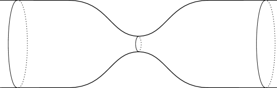
Figure 3.1. An hourglass shaped surface of revolution.

Suppose $V=h^{2}V_{W}$, with $V_{W}=V_{W}(r)\in C_{c}^{\infty}((-R,R))$. Then the part of the trapped set away from the cylindrical ends is normally hyperbolic and we have (3.10) (see [DyZw, (6.3.10)], and see also [ChWu, Ch3] for the case of a degenerate minumum where incidentally we also have (3.3)). Consequently, by Theorem 3.1, there is $z_{0}>0$ such that for all $s_{1},\ s_{2}>1/2$ such that $s_{1}+s_{2}>2$, there is $C>0$ such that

$$\|(1+|r|)^{-s_{1}}(-\Delta+V_{W}-z)^{-1}(1+|r|)^{-s_{2}}\|_{L^{2}(X)\to L^{2}(X)}\leq C,$$

for all $z\in\mathbb{C}$ with $\operatorname{Re}z\geq z_{0}$ and $\operatorname{Im}z\neq 0$. In particular the spectrum of $-\Delta+V_{W}$ is absolutely continuous on $(z_{0},\infty)$.

But if $f$ and $V_{W}$ are suitably chosen, then $\Delta+V_{W}$ has an eigenvalue embedded in the spectrum in $[0,z_{0}]$. Indeed, we have

$$\Delta=f(r)^{-1}\left(\sum_{j=0}^{\infty}\left(\partial_{r}^{2}-f^{\prime\prime}(r)f(r)^{-1}-\sigma^{2}_{j}f(r)^{-4/(d-1)}\right)\phi\otimes\phi\right)f(r),$$

where $\{\phi_{j}\}_{j=0}^{\infty}$ is a complete set of real-valued orthonormal eigenfunctions of the Laplacian on $Y$ and $-\Delta_{Y}\phi_{j}=\sigma_{j}^{2}\phi_{j}$. For $J\in\mathbb{N}_{0}$, consider the effective potential

$$V_{J}(r):=f^{\prime\prime}(r)f(r)^{-1}+\sigma^{2}_{J}(f(r)^{-4/(d-1)}-1)+V_{W}(r).$$

Then $D_{r}^{2}+V_{J}$ has an eigenvalue as long as $\int V_{J}(r)dr\leq 0$ by [ReSi, Theorem XIII.110], and this corresponds to an embedded eigenvalue for $-\Delta+V_{W}$ as long as it is positive, for which it suffices to have $\min V_{J}(r)>-\sigma^{2}_{J}$. For example, we may take $f$ such that $\int(f(r)^{-4/(d-1)}-1)\leq 1/4$ and $V_{W}\in C_{c}^{\infty}((-R,R);[-\sigma_{J}^{2}/2,0])$ such that $V_{W}(r)=-\sigma_{J}^{2}/2$ on $[-R/2,R/2]$, and then $J$ sufficiently large.

By elaborating the above constuction one can also find examples with any finite number of embedded eigenvalues.

It is not clear whether there are examples of manifolds with cylindrical ends such that $-\Delta$ has a finite but nonzero number of eigenvalues. For all known examples where eigenvalues occur, the existence of infinitely many eigenvalues is either also established [ChZw, Pa2] or at the least it is not ruled out [KrKř]. On the other hand $0$ is always a resonance of $-\Delta$ on a manifold with cylindrical ends, with the constant functions as resonant states, unless there is a boundary condition somewhere that eliminates them.

4. Proof of Theorems 3.1 and 3.2

4.1. Outline of proof

The idea of the proofs is to define a parametrix for $P-z$ by

$$G:=\chi_{K}(r-1)(P-iW_{K}(r)-z)^{-1}\chi_{K}(r)+\chi_{e}(r+1)(P_{e}-z)^{-1}\chi_{e}(r),$$ (4.1)

where $\chi_{e},\chi_{K}\in C^{\infty}(\mathbb{R})$ obey $\chi_{e}+\chi_{K}=1$, $\operatorname{supp}\chi_{e}\subset(3,\infty)$, and $\operatorname{supp}\chi_{K}\subset(-\infty,4)$, and $P_{e}$ is a suitably chosen differential operator such that $P_{e}=P$ on the part of $X$ where $r>2$. Then

$$(P-z)G=I+[h^{2}D_{r}^{2},\chi_{K}(r-1)](P-iW_{K}(r)-z)^{-1}\chi_{K}(r)+[h^{2}D_{r}^{2},\chi_{e}(r+1)](P_{e}-z)^{-1}\chi_{e}(r),$$

and we will construct an inverse for $(P-z)$ by removing this remainder using a Neumann series; although the remainder above need not be small, we will see that powers of it are. We call the part of $X$ where $r\in(2,5)$ the resolvent gluing region, because the functions in the range of the remainder are supported in that region. To prove that powers of the remainder are small, we will need to know that:

1. The resolvents of $P-iW_{K}(r)$ and $P_{e}$ obey estimates analogous to (3.4) and (3.6). This is the case for $P-iW_{K}(r)$ thanks to the assumption (3.3), and we will prove it for a suitable choice of $P_{e}$ in §4.3 and §4.4.

2. The resolvents of $P-iW_{K}(r)$ and $P_{e}$ obey improved estimates when multiplied by cutoffs with suitable support properties in the resolvent gluing region, corresponding to a (special case of a) semiclassically outgoing condition so that we are able to remove the remainders. The needed estimates are proved in [DaVa1] for $P-iW_{K}(r)$ and in §4.3 and §4.4 for $P_{e}$.

We combine these estimates to prove Theorems 3.1 and 3.2 in §4.5. There we follow a procedure analogous to that in [DaVa1], but with some finer analysis of remainders to remove the losses due to trapping in the cylindrical end (see also [Da2, §3] for another, in some ways related, variation on this resolvent gluing procedure).

4.2. Model operators for $X_{e}$

On $X_{e}$, $\Delta$ can be written as a direct sum of one-dimensional Schrödinger operators:

$$\Delta|_{X_{e}}=f(r)^{-1}\left(\sum_{j=0}^{\infty}\left(\partial_{r}^{2}-f^{\prime\prime}(r)f(r)^{-1}-\sigma^{2}_{j}f(r)^{-4/(d-1)}\right)\phi\otimes\phi\right)f(r),$$

where $\{\phi_{j}\}_{j=0}^{\infty}$ is a complete set of real-valued orthonormal eigenfunctions of the Laplacian on $Y$ and $-\Delta_{Y}\phi_{j}=\sigma_{j}^{2}\phi_{j}$. We will introduce model operators $P_{j}$ obeying

$$P_{j}|_{[2,\infty)}=-h^{2}\partial_{r}^{2}+V_{j}(r),\qquad V_{j}(r):=V(r)+h^{2}f^{\prime\prime}(r)f(r)^{-1}+h^{2}\sigma_{j}^{2}(f(r)^{-4/(d-1)}-1),$$ (4.2)

and we will be studying them near the energy levels

$$E_{j}:=E_{0}-h^{2}\sigma_{j}^{2}.$$

We will study two ranges of $j$ separately, and the model operators $P_{j}$ will act on different spaces depending on $j$. These two ranges correspond to different behavior in the resolvent gluing region, which is the part of $X$ where $r\in(2,5)$ (see §4.1). To define the ranges, fix $E_{*}\in\mathbb{R}$, independent of $h$, such that

$$0<E_{*}\leq c_{\mathcal{J}},$$

where $c_{\mathcal{J}}$ is as in the statement of Theorem 3.2, and

$$E_{j}\leq E_{*}\Longrightarrow h^{2}\sigma_{j}^{2}f(5)^{-4/(d-1)}\geq E_{0};$$ (4.3)

note that the conditions are compatible because $E_{j}=0$ when $E_{0}=h^{2}\sigma_{j}^{2}$ and $f(5)<1$.

The first range we consider is $E_{j}\leq E_{*}$; in this range the set where $r<5$ is classically forbidden because $V_{j}>E_{j}$, and we control remainders in the gluing region using Agmon estimates, taking care to prove that our estimates are uniform as $j\to\infty$ (although the effective potentials $V_{j}$ become unbounded as $j\to\infty$, they are nonnegative, so the relevant estimates actually get better in this limit). The second range is $E_{j}\geq E_{*}$; in this range the set where $r<5$ is not classically forbidden, but the energy levels $E_{j}$ are bounded below by a positive constant and the effective potentials $V_{j}$ are repulsive, so nontrapping propagation of singularities estimates hold, which we can use to control the remainders in the gluing region (once again we take care to prove that the estimates are uniform in $j$).

For the first range of $j$ we define the operators $P_{j}$ to act on $L^{2}(\mathbb{R}_{+})$, with a Dirichlet boundary condition at $0$, in order to be able to use Theorem 1.3 (the Dirichlet boundary condition makes it easier to analyze the behavior of the resolvent when $|E_{j}|$ is small). For the second range of $j$ it is more convenient to work over $\mathbb{R}$ than $\mathbb{R}_{+}$, in order to avoid reflection phenomena when studying propagation of singularities.

4.3. Analysis when $E_{j}\leq E_{*}$

In §4.3 all function norms and inner products are in $L^{2}(\mathbb{R}_{+})$, and operator norms are $L^{2}(\mathbb{R}_{+})\to L^{2}(\mathbb{R}_{+})$, unless otherwise specified.

For this range of $j$, we put

$$P_{j}:=h^{2}D_{r}^{2}+V_{j}(r),$$ (4.4)

regarded as a self-adjoint operator on $L^{2}(\mathbb{R}_{+})$ with a Dirichlet boundary condition at $r=0$.

We first prove resolvent estimates for $P_{j}$ analogous to (3.4) and (3.6).

Proposition 4.1.

Fix $s_{1},\ s_{2},\ s>1/2$ such that $s_{1}+s_{2}>2$. Then

$$\|(1+r)^{-s_{1}}(P_{j}-E_{j}-i\varepsilon)^{-1}(1+r)^{-s_{2}}\|\leq Ch^{-2},$$ (4.5)

and

$$\|(1+r)^{-s}\chi(r)(P_{j}-E_{j}-i\varepsilon)^{-1}(1+r)^{-s}\|+\|(1+r)^{-s}(P_{j}-E_{j}-i\varepsilon)^{-1}\chi(r)(1+r)^{-s}\|\leq Ch^{-1},$$ (4.6)

for all $\varepsilon\in\mathbb{R}\setminus 0$, $j\in\mathbb{N}$ such that $E_{j}\leq E_{*}$, where

$$\chi(r)=\sqrt{V_{L}(r)+f(r)^{-4/(d-1)}-1}.$$

Proof.

The idea of the proof is to apply Theorem 1.3; more precisely (4.5) corresponds to (1.8) (see also (1.5)), and (4.6) corresponds to (1.9) (see also (1.6)).

Before beginning the proof proper, by way of outline let us briefly discuss the terms in $V_{j}$, and explain how they each do or do not satisfy (1.3). The term $h^{2}\sigma_{j}^{2}(f(r)^{-4/(d-1)}-1)$ does satisfy it thanks to (3.2) and (4.3), and moreover those bounds and $f(r)<1$ for $r<6$ imply that the term is nontrivial when $r<6$. The term $V_{L}$ satisfies it, and we think of it as being harmless. The terms $V_{S}$ does not satisfy it, but we will show that its effect is compensated by that of the $h^{2}\sigma_{j}^{2}(f(r)^{-4/(d-1)}-1)$ term. The most difficult term to treat is the $h^{2}f^{\prime\prime}(r)f(r)^{-1}$ term. This term may prevent $h^{-2}V_{j}$ from satisfying (1.3), but we will show that thanks to (4.3) we can treat it as a small perturbation.

More precisely, let

$$V_{M}(r):=V_{j}(r)-h^{2}f^{\prime\prime}(r)f(r)^{-1},$$

and observe that for $h$ sufficiently small $V_{M}$ obeys (1.3) for some $\delta_{V}>0$, since $V_{L}$ and $f^{-4/(d-1)}-1$ obey it and $|V_{S}|+|V_{S}^{\prime}|\leq C(f^{-4/(d-1)}-1)$ thanks to (4.3). Indeed, to see that $f^{-4/(d-1)}-1$ obeys it we write, using $\alpha:=4/(d-1)$ and (3.2),

$$-(f(r)^{-\alpha}-1)^{\prime}=\alpha f^{\prime}(r)f(r)^{-\alpha-1}\geq\alpha\delta_{0}\frac{f(r)^{-\alpha-1}-f(r)^{-\alpha}}{1+r}\geq\frac{f(r)^{-\alpha}-1}{C(1+r)},$$

where we also used the fact that if $a<b$ then

$$C^{-1}(1-f)\leq f^{a}-f^{b}\leq C(1-f).$$ (4.7)

Hence by (1.8) with $V_{D}=h^{-2}V_{M}$, we have

$$\|(1+r)^{-s_{1}}(h^{2}D_{r}^{2}+V_{M}-E_{j}-i\varepsilon)^{-1}(1+r)^{-s_{2}}\|\leq Ch^{-2}.$$ (4.8)

Note that by the resolvent identity

$$\begin{split}(1+r)^{-s_{1}}(P_{j}-E_{j}&-i\varepsilon)^{-1}(1+r)^{-s_{2}}=(1+r)^{-s_{1}}(h^{2}D_{r}^{2}+V_{M}-E_{j}-i\varepsilon)^{-1}(1+r)^{-s_{2}}\\ &\times\sum_{k=0}^{\infty}\left[-(1+r)^{s_{2}}h^{2}f^{\prime\prime}(r)f(r)^{-1}(h^{2}D_{r}^{2}+V_{M}-E_{j}-i\varepsilon)^{-1}(1+r)^{-s_{2}}\right]^{k},\end{split}$$ (4.9)

the proof of (4.5) is reduced to the proof of

$$\|(1+r)^{s_{2}}h^{2}f^{\prime\prime}(r)f(r)^{-1}(h^{2}D_{r}^{2}+V_{M}-E_{j}-i\varepsilon)^{-1}(1+r)^{-s_{2}}\|\leq 1/2.$$ (4.10)

But by (1.9), with $\theta=1$ and $V_{D}=h^{-2}V_{M}\geq h^{-2}(f^{-4/(d-1)}-1)/C$ (again using (4.3)), we have

$$\|(f(r)^{-4/(d-1)}-1)^{\frac{1}{2}}(1+r)^{-\frac{1}{2}}(h^{2}D_{r}^{2}+V_{M}-E_{j}-i\varepsilon)^{-1}(1+r)^{-s_{2}}\|\leq Ch^{-1},$$

and interpolating this with (4.8) gives

$$\|(f(r)^{-4/(d-1)}-1)^{\frac{1}{4}}(1+r)^{-\frac{s_{1}}{2}-\frac{1}{4}}(h^{2}D_{r}^{2}+V_{M}-E_{j}-i\varepsilon)^{-1}(1+r)^{-s_{2}}\|\leq Ch^{-3/2}.$$

Hence to prove (4.10), and consequently also (4.5), it is enough to show that

$$(1+r)^{s_{2}}|f^{\prime\prime}(r)|\leq C(f(r)^{-4/(d-1)}-1)^{\frac{1}{4}}(1+r)^{-\frac{s_{1}}{2}-\frac{1}{4}}.$$ (4.11)

To prove (4.11) we will use the fact that any bounded $\varphi\in C^{2}([r,\infty);[0,\infty))$ satisfies

$$|\varphi^{\prime}(r)|^{2}\leq 2\sup\varphi\sup|\varphi^{\prime\prime}|,$$ (4.12)

where the suprema are taken over $[r,\infty)$. Indeed, by Taylor’s theorem, for every $t\geq 0$ there is $t_{0}\in[r,r+t]$ such that

$$t|\varphi^{\prime}(r)|=|\varphi(r+t)-\varphi(r)-t^{2}\varphi^{\prime\prime}(t_{0})/2|\leq\sup\varphi+t^{2}\sup|\varphi^{\prime\prime}|/2,$$

and taking $t=|\varphi^{\prime}(r)|/\sup|\varphi^{\prime\prime}|$ gives (4.12). Applying (4.12) once with $\varphi=f^{\prime}$ and once with $\varphi=1-f$ gives

$$|f^{\prime\prime}(r)|^{4}\leq 4\sup|f^{\prime}|^{2}\sup|f^{\prime\prime\prime}|^{2}\leq 8\sup(1-f)\sup|f^{\prime\prime}|\sup|f^{\prime\prime\prime}|^{2}=8(1-f(r))\sup|f^{\prime\prime}|\sup|f^{\prime\prime\prime}|^{2},$$

where the suprema are still all taken over $[r,\infty)$. Applying (3.1) gives

$$|f^{\prime\prime}(r)|\leq C(1-f(r))^{\frac{1}{4}}(1+r)^{-2-\frac{3\delta_{0}}{4}}.$$

By (4.7) this implies (4.11) as long as $s_{1}+2s_{2}\leq(7+3\delta_{0})/2$, which we may suppose without loss of generality. This completes the proof of (4.5).

The proof of (4.6) proceeds along similar lines. Applying (4.9) with $s_{1}=s_{2}=s$ allows us to reduce the proof of the bound on the first term in (4.6) to the proof of

$$\|(1+r)^{-s}\chi(r)(h^{2}D_{r}^{2}+V_{M}-E_{j}-i\varepsilon)^{-1}(1+r)^{-s}\|\leq Ch^{-1}.$$ (4.13)

But (4.13) follows from (1.9) with $\theta=1$ and $V_{D}=h^{-2}V_{M}\geq h^{-2}(V_{L}+f^{-4/(d-1)}-1)/C=h^{-2}\chi^{2}/C$. The bound on the second term of (4.6) follows from the bound on the first term after taking the adjoint. ∎

We will also need the following Agmon estimates:

Proposition 4.2.

Let $R\in(0,5]$, $\chi_{-}\in C_{c}^{\infty}((0,R)),\ \chi_{+}\in C_{c}^{\infty}((R,\infty)),$ and $s>1/2$. Then

$$\|\chi_{-}(P_{j}-E_{j}-i\varepsilon)^{-1}(1+r)^{-s}\|_{L^{2}(\mathbb{R}_{+})\to H^{1}_{h}(\mathbb{R}_{+})}+\|(1+r)^{-s}(P_{j}-E_{j}-i\varepsilon)^{-1}\chi_{-}\|\leq C,$$ (4.14)

$$\|\chi_{-}(P_{j}-E_{j}-i\varepsilon)^{-1}\chi_{+}\|\leq e^{-1/(Ch)},$$ (4.15)

for all $\varepsilon\in\mathbb{R}\setminus 0$, and $j\in\mathbb{N}$ such that $E_{j}\leq E_{*}$.

Recall that the norms without subscripts are $L^{2}(\mathbb{R}_{+})\to L^{2}(\mathbb{R}_{+})$ here, and that $\chi_{-}$ is supported in the classically forbidden region for $P_{j}-E_{j}$.

Proof.

These are similar to the usual Agmon estimates as in [Zw1, §7.1] but we keep track of the $j$ dependence.

Let $v\in L^{2}(\mathbb{R}_{+})$, and let $u:=(P_{j}-E_{j}-i\varepsilon)^{-1}(1+r)^{-s}v$. Fix $\varphi_{0}\in C_{c}^{\infty}((0,R);[0,1])$ which is identically 1 on a neighborhood $I$ of $\operatorname{supp}\chi_{-}$, and let $\varphi(r):=m\varphi_{0}(r)$, for a constant $m$ to be chosen later. Then define

$$\begin{split}P_{\varphi}:&=e^{\varphi/h}(P_{j}-E_{j}-i\varepsilon)e^{-\varphi/h}\\ &=h^{2}D_{r}^{2}+2i\varphi^{\prime}hD_{r}+V_{j}-\varphi^{\prime 2}+h\varphi^{\prime\prime}-E_{j}-i\varepsilon.\end{split}$$

Put $w:=\chi_{0}e^{\varphi/h}u$, where $\chi_{0}\in C_{c}^{\infty}((0,R))$ is 1 near $\operatorname{supp}\varphi$. Using $\operatorname{Re}\langle 2h\varphi^{\prime}w^{\prime},w\rangle=-h\langle\varphi^{\prime\prime}w,w\rangle$, write

$$\operatorname{Re}\langle P_{\varphi}w,w\rangle=\|hw^{\prime}\|^{2}+\langle(V_{j}-\varphi^{\prime 2}-E_{j})w,w\rangle.$$

We now observe that, using (4.3) and the fact that $1-f(r)^{-4/(d-1)}>1-f(5)^{-4/(d-1)}>0$ for $r\in(0,5)$, we can choose $m>0$ small enough, independent of $h$ and $j$, such that there is $c_{0}>0$ independent of $h$ and $j$ for which $V_{j}-\varphi^{\prime 2}-E_{j}>c_{0}$ on $\operatorname{supp}w$ for $h$ small enough. This implies

$$\|w\|\leq C\|P_{\varphi}w\|\leq C\|e^{\varphi/h}\chi_{0}v\|+C\|[P,\chi_{0}]u\|,$$

where we used $\varphi\chi_{0}^{\prime}=0$ to deduce $[P_{\varphi},\chi_{0}]e^{\varphi/h}u=[P,\chi_{0}]u$. We use an elliptic estimate to bound the commutator term: for $\chi_{1}\in C_{c}^{\infty}((0,R))$ we have, using $V_{j}-E_{j}\geq V_{0}-E_{0}\geq-C$,

$$\begin{split}C\|\chi_{1}v\|\|\chi_{1}u\|&\geq\operatorname{Re}\langle(1+r)^{-s}v,\chi_{1}^{2}u\rangle=\operatorname{Re}\langle(P_{j}-E_{j})u,\chi_{1}^{2}u\rangle\\ &\geq\|\chi_{1}hu^{\prime}\|^{2}-Ch\|\chi_{1}hu^{\prime}u\|_{L^{1}(\mathbb{R}_{+})}-C\|\chi_{1}u\|^{2},\end{split}$$ (4.16)

from which it follows that, provided $\chi_{2}=1$ near $\operatorname{supp}\chi_{0}$,

$$\|[P,\chi_{0}]u\|\leq Ch\|\chi_{2}u\|+Ch\|\chi_{2}v\|\leq Ch^{-1}\|v\|,$$

where we used (4.5). Consequently

$$\int_{I}|u|^{2}=e^{-2m/h}\int_{I}|w|^{2}\leq Ce^{-2m/h}\left(\|e^{\varphi/h}\chi_{0}v\|^{2}+h^{-2}\|v\|^{2}\right)\leq C\|v\|^{2},$$ (4.17)

where we used $\varphi\leq m$.

To estimate $u^{\prime}$ we apply (4.16) with $\chi_{1}\in C_{c}^{\infty}(I)$, giving

$$\|\chi_{1}hu^{\prime}\|^{2}\leq C\left(\int_{I}|u|^{2}dr+\|\chi_{1}hv\|^{2}\right),$$

which implies the bound on the first term of (4.14). The bound on the second term follows from taking the adjoint, and (4.15) follows from the fact that if $\operatorname{supp}v\subset(R,\infty)$, then $\chi_{0}v=0$ and we can improve (4.17) to

$$\int_{I}|u|^{2}=e^{-2m/h}\int_{I}|w|^{2}\leq Ce^{-2m/h}h^{-2}\|v\|^{2}.$$

∎

4.4. Analysis when $E_{j}>E_{*}$

In §4.4 all function norms and inner products are in $L^{2}(\mathbb{R})$, and operator norms are $L^{2}(\mathbb{R})\to L^{2}(\mathbb{R})$, unless otherwise specified.

For this range of $j$ the Agmon estimate (4.15) must be replaced by a propagation of singularities estimate. It is convenient to introduce a complex absorbing barrier and to work over $\mathbb{R}$: let $W_{e}\in C^{\infty}(\mathbb{R};[0,1])$ be $1$ near $(-\infty,1]$ and $0$ near $[2,\infty)$, and let

$$V_{j,0}:=\chi_{0}V_{j},$$

where $\chi_{0}\in C^{\infty}(\mathbb{R};[0,1])$ is $0$ near $(-\infty,0]$ and $1$ near $[1,\infty)$. We now put

$$P_{j}:=h^{2}D_{r}^{2}+V_{j,0}(r)-iW_{e}(r),$$

regarded as an unbounded operator on $L^{2}(\mathbb{R})$ with domain $H^{2}(\mathbb{R})$. We will prove

Proposition 4.3.

For any $s>1/2$ we have

$$\|(1+r_{+})^{-s}(P_{j}-E_{j}-i\varepsilon)^{-1}(1+r_{+})^{-s}\|\leq Ch^{-1},$$ (4.18)

where $r_{+}:=\max\{0,r\}$. For any $\chi_{-}\in C_{c}^{\infty}((0,3)),\ \chi_{+}\in C_{c}^{\infty}((3,\infty)),\ \psi\in C_{c}^{\infty}((0,\infty))$, we have

$$\|\chi_{-}(r)(P_{j}-E_{j}-i\varepsilon)^{-1}\chi_{+}(r)\psi(hD_{r})\|=O(h^{\infty}).$$ (4.19)

Both (4.18) and (4.19) hold uniformly for all $\varepsilon>0$, and for all $j\in\mathbb{N}_{0}$ such that $E_{j}>E_{*}$.

Note that since $E_{j}$ is bounded from below away from 0, we can think of (4.18) as the analogue of (1.7) in this setting; we do not need a weight for $r<0$ because the $-iW_{e}$ term makes the operator $P_{j}-E_{j}-i\varepsilon$ semiclassically elliptic there. It is also similar to the usual nontrapping resolvent estimate as in [VaZw] and in other papers cited therein, but we need an estimate which is uniform in $j$.

The propagation of singularities estimate (4.19) is a microlocalized version of (4.18). The improved bound is due to the fact that solutions to the classical equations of motion $\dot{r}=2\rho$, $\dot{\rho}=-V^{\prime}_{j}(r)$ with $r(0)>3$ and $\rho(0)>0$ cannot have $r(t)<3$ for any $t>0$.

Proof of (4.18).

We prove (4.18) using a microlocal positive commutator argument, rather than (as is probably possible) integration by parts arguments as in the proof of (1.7). We do this because the proof of (4.19) follows along very similar lines, and the latter estimate does not seem to be provable by integration by parts arguments. The idea is to construct a microlocal commutant, based on the $w(r)\partial_{r}$ of the proof of (1.7), but which is nonnegative. This will be obtained as the quantization of an escape function, defined in (4.26) below.

As in [VaZw] we will use the semiclassical scattering calculus, and we begin by recalling its relevant properties. We use $(r,\rho)$ to denote points in $T^{*}\mathbb{R}$, and for $l,\ m\in\mathbb{R}$ we define the symbol class $S^{m}_{l}$ to be the set of $a\in C^{\infty}(T^{*}\mathbb{R})$ such that, for any $n_{1},\ n_{2}\in\mathbb{N}_{0}$ there is $C_{n_{1},n_{2}}$ such that

$$|\partial^{n_{1}}_{r}\partial^{n_{2}}_{\rho}a(r,\rho)|\leq C_{n_{1},n_{2}}(1+|r|)^{l-n_{1}}(1+|\rho|)^{m-n_{2}},$$ (4.20)

for all $(r,\rho)\in T^{*}\mathbb{R}$. We also write $S^{\infty}_{l}:=\bigcup_{m}S^{m}_{l}$, $S^{-\infty}_{l}:=\bigcap_{m}S^{m}_{l}$, and similarly for $S^{m}_{\infty}$ and $S^{m}_{-\infty}$. Below we will consider symbols depending on $h$ and $j$, and the constants $C_{n_{1},n_{2}}$ in (4.20) will always be uniform with respect to those parameters. For such $a$, we denote the semiclassical quantization by $\operatorname{Op}_{h}(a)$, which we define by

$$\operatorname{Op}_{h}(a)u:=\frac{1}{2\pi h}\int\!\!\!\int e^{i(r-r^{\prime})\rho/h}a(r,\rho)u(r^{\prime})dr^{\prime}d\rho.$$ (4.21)

When a symbol is denoted by a lowercase letter (with possible subscripts and superscripts), we will denote its quantization by the corresponding uppercase letter (with the same subscripts and superscripts, if any).

We recall the composition and adjoint formulas. If $a\in S^{m_{1}}_{l_{1}}$ and $b\in S^{m_{2}}_{l_{2}}$, then there is $a\#b\in S^{m_{1}+m_{2}}_{l_{1}+l_{2}}$ such that

$$AB=\operatorname{Op}_{h}(a\#b),$$

and, for any $N\in\mathbb{N}$,

$$\begin{split}a\#b(r,\rho)&=e^{-ih\partial_{r^{\prime}}\partial_{\rho^{\prime}}}\left(a(r,\rho^{\prime})b(r^{\prime},\rho)\right)\Big{|}_{(r,\rho)=(r^{\prime},\rho^{\prime})}\\ &=\sum_{k=0}^{N-1}\frac{(-ih)^{k}}{k!}\partial_{\rho}^{k}a(r,\rho)\partial_{r}^{k}b(r,\rho)+h^{N}z_{N}(r,\rho),\end{split}$$ (4.22)

where $z_{N}\in S^{m_{1}+m_{2}-N}_{l_{1}+l_{2}-N}$ is given by

$$\begin{split}z_{N}(r,\rho):=\frac{(-i)^{N}}{(N-1)!}\int_{0}^{1}(1-t)^{N-1}e^{-ith\partial_{r^{\prime}}\partial_{\rho^{\prime}}}\left(\partial_{\rho^{\prime}}^{N}a(r,\rho^{\prime})\partial_{r^{\prime}}^{N}b(r^{\prime},\rho)\right)\Big{|}_{(r,\rho)=(r^{\prime},\rho^{\prime})}dt.\end{split}$$ (4.23)

Indeed, [Zw1, Theorem 4.14] gives the formula for Schwartz symbols, and [Zw1, Theorems 4.13 and 4.18] give it for a larger class of symbols than the ones we consider, but with weaker bounds on $z_{N}$. The statement that $z_{N}\in S^{m_{1}+m_{2}-N}_{l_{1}+l_{2}-N}$ follows from applying [Zw1, Theorem 4.17] to (4.23). See also [DyZw, Proposition E.8], [Pa1, (3) and (9)], [Sh], and [Hö, §18.5] for similar expansions, and [HeSj] for a much more general version.

Similarly, if $a\in S^{m}_{l}$ there is $a^{*}\in S^{m}_{l}$ such that the formal adjoint of $A$ is given by

$$A^{*}=\operatorname{Op}_{h}(a^{*}),$$

and, for any $N\in\mathbb{N}$,

$$a^{*}(r,\rho)=e^{-ih\partial_{r}\partial_{\rho}}\bar{a}(r,\rho)=\sum_{k=0}^{N-1}\frac{(-ih)^{k}}{k!}\partial_{r}^{k}\partial_{\rho}^{k}\bar{a}(r,\rho)+h^{N}z_{N}(r,\rho),$$ (4.24)

where this time $z_{N}\in S^{m-N}_{l-N}$ is given by

$$z_{N}(r,\rho):=\frac{(-i)^{N}}{(N-1)!}\int_{0}^{1}(1-t)^{N-1}e^{-ith\partial_{r}\partial_{\rho}}\partial_{r}^{N}\partial_{\rho}^{N}\bar{a}(r,\rho)dt.$$

Let

$$p_{j}:=\rho^{2}+V_{j,0}(r)-iW_{e}(r)$$

be the semiclassical symbol of $P_{j}$ (in the sense that $p_{j}\in S^{2}_{0}$ and $P_{j}=\operatorname{Op}_{h}(p_{j})$), let

$$R_{j}:=\inf\{r>0\mid\textrm{both }V_{j}(r)=V_{j,0}(r)\textrm{ and }V_{j,0}(r)\leq E_{*}/2\},$$

so that $R_{0}\leq R_{1}\leq\cdots$, and let

$$F_{j}:=\{(r,\rho)\mid r\geq 1\textrm{ and }\rho^{2}\leq 2E_{0}\}\setminus\{(r,\rho)\mid R_{j}<r\textrm{ and }\rho^{2}<E_{*}/3\}.$$

Note that each $F_{j}$ is a closed neighborhood of the energy surface $p_{j}=E_{j}$, and they have been chosen such that they form a nested sequence $F_{0}\subset F_{1}\subset\cdots$. Moreover, since we only consider $j$ such that $E_{j}>E_{*}$, all of the $F_{j}$ agree outside of a compact set: see Figure 4.1.

$r$ [l] at 239 87 $r$ [l] at 596 87 $\rho$ [l] at 17 195 $\rho$ [l] at 374 195 $R_{j}$ [l] at 96 87 $1$ [l] at 24 87 $\sqrt{E_{*}/3}$ [l] at -50 120 $\sqrt{2E_{0}}$ [l] at -35 180 $\textrm{the case }R_{j}>1$ [l] at 74 -15 $\textrm{the case }R_{j}<1$ [l] at 431 -15                    

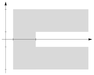
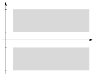
Figure 4.1. The shaded regions are the sets $F_{j}$. They are closed nested neighborhoods of the energy surfaces $p_{j}=E_{j}$ which agree outside of a compact set.

Observe that we have $|p_{j}-E_{j}-i\varepsilon|\geq c(1+\rho^{2})$ on $T^{*}\mathbb{R}\setminus F_{j}$, for some $c>0$, which implies the following elliptic estimate: for any $a\in S^{m}_{l},\ a^{\prime}\in S^{m-2}_{l}$ satisfying $\operatorname{supp}a\cap F_{j}=\varnothing$ and $|a^{\prime}(r,\rho)|\geq(1+|r|)^{l}(1+|\rho|)^{m-2}$ for $(r,\rho)\in\operatorname{supp}a$, and for any $N\in\mathbb{R}$, we have

$$\|Au\|\leq C\|A^{\prime}(P_{j}-E_{j}-i\varepsilon)u\|+h^{N}\|Z_{N}u\|,$$ (4.25)

for some $z_{N}\in S^{m-N}_{l-N}$. This follows from (4.22) by the usual iterative elliptic parametrix construction as in [DyZw, Theorem E.32].

To handle $F_{j}$, we define an escape function (based on the usual $-r\rho$ but modified to be nonnegative near $F_{j}$ and more slowly growing) as follows. For $\delta\in(0,1/4)$, take $\tilde{q}_{\delta}\in C^{\infty}(\mathbb{R})$ with $\tilde{q}_{\delta}(x)=x^{\delta}$ for $x\geq 2$, $\tilde{q}_{\delta}(x)=|x|^{-\delta}$ for $x\leq-2$, and $\tilde{q}_{\delta}^{\prime}(x)>0$ for $|x|<2$, and put

$$q(r,\rho):=\tilde{q}_{\delta}(-r\rho)\chi_{q}(r,\rho),$$ (4.26)

where $\chi_{q}\in S^{-\infty}_{0}$ is real valued, is $1$ near all of the $F_{j}$, and vanishes in a neighborhood of

$$\{(r,\rho)\mid r\not\in(-1,1+\max_{j}R_{j})\textrm{ and }\rho=0\}$$

whose boundary consists of two line segments and four half lines as in Figure 4.2.

$r$ [l] at 239 25 $\rho$ [l] at 43 70 $-1$ [l] at 10 25 $1+\max_{j}\!R_{j}$ [l] at 100 23

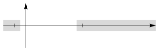
Figure 4.2. The kind of neighborhood where $\chi_{q}$ must vanish.

Then $q\in S^{-\infty}_{\delta}$, and near $F_{j}$ we have

$$\{\operatorname{Re}p_{j},q^{2}\}=2(-2\rho^{2}+rV^{\prime}_{j}(r))\tilde{q}_{\delta}^{\prime}(-r\rho)\tilde{q}_{\delta}(-r\rho)\leq-cr^{-1-2\delta},$$ (4.27)

for some $c>0$ (here we used $V_{j}\geq E_{*}/2\Longrightarrow rV^{\prime}_{j}\leq-1/C$).

Consequently, there are real valued symbols $b\in S^{-\infty}_{-\frac{1}{2}+\delta}$ and $a_{0}\in S^{-\infty}_{-1+2\delta}$ such that

$$b^{2}=\{q^{2},\operatorname{Re}p_{j}\}+a_{0},$$ (4.28)

and such that $\operatorname{supp}a_{0}\cap F_{j}=\varnothing$ and $b\geq cr^{-\frac{1}{2}-\delta}>0$ near $F_{j}$; for example we can take $b:=\{q^{2},\operatorname{Re}p_{j}\}^{1/2}\chi_{b}$ for some $\chi_{b}\in S^{-\infty}_{0}$ with $\chi_{b}=1$ near $F_{j}$ and supported in the set where (4.27) holds. Note that $q$ depends on $\delta$, and $b$ and $a_{0}$ depend on $\delta$ and $j$, although our notation does not reflect this.

Using (4.28), (4.22), and (4.24), we can write

$$B^{*}B=\frac{i}{h}[Q^{*}Q,\operatorname{Re}P_{j}]+A_{0}+hA_{1},$$

for some $a_{1}\in S^{-\infty}_{-2+2\delta}$, giving

$$\|Bu\|^{2}=\frac{i}{h}\langle[Q^{*}Q,\operatorname{Re}P_{j}]u,u\rangle+\langle A_{0}u,u\rangle+h\langle A_{1}u,u\rangle,$$

Combining this with (4.25) and the similar elliptic estimate

$$\|B^{\prime}u\|\leq C\|Bu\|+h^{N}\|Z_{N}u\|,$$ (4.29)

which holds for all $b^{\prime}\in S^{-\infty}_{-\frac{1}{2}-\delta}$ which is supported in a small enough neighborhood of $F_{j}$ and for suitable $z_{N}\in S^{-\infty}_{-\frac{1}{2}-\delta-N}$, we have (since $\delta<1/4$),

$$\|(1+r_{+})^{-\frac{1}{2}-\delta}u\|^{2}\leq C\frac{i}{h}\langle[Q^{*}Q,\operatorname{Re}P_{j}]u,u\rangle+C\|(P_{j}-E_{j}-i\varepsilon)u\|^{2}.$$

Next

$$i\langle[Q^{*}Q,\operatorname{Re}P_{j}]u,u\rangle=-2\operatorname{Im}\langle Q(P_{j}-E_{j}-i\varepsilon)u,Qu\rangle-2\operatorname{Re}\langle Q(W_{e}(r)+\varepsilon)u,Qu\rangle,$$

giving

$$\|(1+r_{+})^{-\frac{1}{2}-\delta}u\|^{2}\leq\frac{C}{h^{2}}\|(1+r_{+})^{\frac{1}{2}+3\delta}(P_{j}-E_{j}-i\varepsilon)u\|^{2}-\frac{C}{h}\operatorname{Re}\langle Q(W_{e}(r)+\varepsilon)u,Qu\rangle.$$

But

$$-\operatorname{Re}\langle Q(W_{e}(r)+\varepsilon)u,Qu\rangle\leq|\operatorname{Re}\langle Q^{*}[Q,W_{e}(r)]u,u\rangle|,$$

thanks to $W_{e}+\varepsilon\geq 0$, and by (4.22) and (4.24) we have $\operatorname{Re}Q^{*}[Q,W_{e}(r)]=h^{2}a_{2}$ for some $a_{2}\in S^{-\infty}_{-\infty}$, giving

$$|\operatorname{Re}\langle Q^{*}[Q,W_{e}(r)]u,u\rangle|=h^{2}\langle A_{2}u,u\rangle.$$

This proves (4.18) with $s=\frac{1}{2}+3\delta$, and taking $\delta>0$ small enough proves it for all $s>1/2$. ∎

Proof of (4.19).

Let

$$u:=(P_{j}-E_{j}-i\varepsilon)^{-1}\chi_{+}(r)\psi(hD_{r})v,$$

with $\|v\|=1$, and fix $\delta\in(0,1/4)$. We will use the following argument by induction to prove (4.19).

The inductive hypothesis is that for a given $k\in\mathbb{R}$ there is a neighborhood $U$ of $F_{j}\setminus(3,\infty)\times(0,\infty)$ such that $\|Au\|\leq Ch^{k}$ for any $a\in S^{-\infty}_{k+\frac{1}{2}-\delta}$ which is supported in $U$.

The inductive step is that there is a (smaller) neighborhood $U^{\prime}$ of $F_{j}\setminus(3,\infty)\times(0,\infty)$ such that

$$\|A^{\prime}u\|\leq Ch^{k+1/2},$$ (4.30)

for any $a^{\prime}\in S^{-\infty}_{k+1+\delta}$ which is supported in $U^{\prime}$.

Let us see first that (4.30) for arbitrary $k$ implies (4.19). Indeed, by the elliptic estimate (4.25), the composition formula (4.22), and the resolvent estimate (4.18), we see that

$$\|A^{\prime\prime}u\|\leq C_{N}h^{N}$$ (4.31)

for any $N\in\mathbb{R}$ and $a^{\prime\prime}\in S^{\infty}_{-\infty}$ such that $\operatorname{supp}a^{\prime\prime}\subset(0,3)\times\mathbb{R}$ and $\operatorname{supp}a^{\prime\prime}\cap F_{j}=\varnothing$. Then we can write

$$\chi_{-}(r)u=\chi_{-}(r)\varphi_{F}(hD_{r})u+\chi_{-}(r)(1-\varphi_{F}(hD_{r}))u$$

for $\varphi_{F}\in C_{c}^{\infty}(\mathbb{R})$ chosen such that (4.30) applies to the first term on the right and (4.31) applies to the second.

We remark in passing that elaborating this argument we can actually show that $u$ is semiclassically trivial everywhere away from the union of two sets (including uniformly as $|r|\to\infty$ and $|\rho|\to\infty$): the first is $\operatorname{supp}\chi_{+}\times\operatorname{supp}\psi$, and the second is $F_{j}\cap(3,\infty)\times(0,\infty)$ which we can think of as a neighborhood of the forward bicharacteristic flowout of the first. Here we are focusing on a more concrete and narrower version of this conclusion which is sufficient for our purposes.

Next observe that the base case (the inductive hypothesis with $k=-1$ and $U=T^{*}\mathbb{R}$) follows from the resolvent estimate (4.18).

It remains to prove (4.30) under the inductive hypothesis. Roughly speaking, we use an escape function which on $F_{j}\setminus(3,\infty)\times(0,\infty)$ agrees with the one used in the proof of (4.18) above, but is adapted to vanish near $\operatorname{supp}\chi_{+}\times\operatorname{supp}\psi$ and $F_{j}\setminus U$. (Note that $F_{j}\setminus U=\varnothing$ when $k=-1$ but that for $k>-1$ we expect $F_{j}\setminus U\neq\varnothing$ in general).

More specifically, to define the escape function, fix $\chi_{k},\psi_{k}\in C^{\infty}(\mathbb{R})$ nondecreasing, and satisfying $\chi_{k}=0$ near $(-\infty,3]$, $\psi_{k}=0$ near $(-\infty,0]$, $\psi_{k}=1$ near $[\sqrt{E_{*}/3},\infty)$, and $\chi_{k}(r)\psi_{k}(\rho)=1$ near $F_{j}\setminus U$. Then let

$$q_{k}(r,\rho):=\tilde{q}_{k+\frac{3}{2}-\delta}(-r\rho)\chi_{q}(r,\rho)(1-\chi_{k}(r)\psi_{k}(\rho)),$$

where $\tilde{q}_{k+\frac{3}{2}-\delta}$ and $\chi_{q}$ are as in (4.26), so that $q_{k}\in S^{-\infty}_{k+\frac{3}{2}-\delta}$. Calculating as in (4.27), we see that near $F_{j}$ we have

$$\{\operatorname{Re}p_{j},q_{k}^{2}\}\leq 0,$$

and near $F_{j}\setminus(3,\infty)\times(0,\infty)$ we have $\chi_{k}(r)\psi_{k}(\rho)=0$ and hence $\{\operatorname{Re}p_{j},q_{k}^{2}\}\leq-cr^{2k+2-2\delta}<0$ (this is slightly better than (4.27) because outside of a compact set we have $\rho<0$ on $F_{j}\setminus(3,\infty)\times(0,\infty)$ and in particular we are staying away from the outgoing part of the energy surface).

Consequently, as before, we can write

$$b_{k}^{2}=\{q_{k}^{2},\operatorname{Re}p_{j}\}+a_{0,k},$$

where $b_{k}\in S^{-\infty}_{k+1-\delta},\ a_{0,k}\in S^{-\infty}_{2k+2-2\delta}$, $\operatorname{supp}b_{k}\ \subset\operatorname{supp}q_{k}$, $\operatorname{supp}a_{0,k}\cap(F_{j}\cup\operatorname{supp}\chi_{+}\times\operatorname{supp}\psi)=\varnothing$, and $b_{k}\geq cr^{k+1-\delta}>0$ near $F_{j}\setminus(3,\infty)\times(0,\infty)$. Hence

$$B_{k}^{*}B_{k}=\frac{i}{h}[Q_{k}^{*}Q_{k},\operatorname{Re}P_{j}]+A_{0,k}+hA_{1,k},$$

for some $a_{1,k}\in S^{-\infty}_{2k+1-2\delta}$. We refine this by using (4.22) and (4.24) to expand $a_{1,k}$ in powers of $h$ up to $h^{N}$ in terms of $b_{k}$, $q_{k}$, $p_{j}$, $a_{0,k}$, and their derivatives, which gives

$$B_{k}^{*}B_{k}=\frac{i}{h}[Q_{k}^{*}Q_{k},\operatorname{Re}P_{j}]+A_{0,k}+hA^{\prime}_{1,k}+h^{N}Z_{N},$$

where $a^{\prime}_{1,k}\in S^{-\infty}_{2k+1-2\delta}$ has $\operatorname{supp}a^{\prime}_{1,k}\subset\operatorname{supp}q_{k}$ and $z_{N}\in S^{-\infty}_{2k+2-2\delta-N}$. Consequently

$$\|B_{k}u\|^{2}=\frac{i}{h}\langle[Q_{k}^{*}Q_{k},\operatorname{Re}P_{j}]u,u\rangle+\langle A_{0,k}u,u\rangle+h\langle A_{1,k}^{\prime}u,u\rangle+h^{N}\langle Z_{N}u,u\rangle.$$

By the elliptic estimate (4.29) with $b_{k}$ in place of $b$ we see that to deduce (4.30) it is enough to show

$$\|B_{k}u\|^{2}\leq Ch^{2k+1}.$$ (4.32)

Now $\langle A_{0,k}u,u\rangle=O(h^{\infty})$ by (4.25). Also, since $q_{k}$ vanishes near $F_{j}\setminus U$, it follows that $a_{1,k}^{\prime}$ vanishes near $F_{j}\setminus U$, so by (4.25), (4.22), and the inductive hypothesis, we have

$$|\langle A_{1,k}^{\prime}u,u\rangle|\leq Ch^{2k}.$$

Hence to show (4.32) it suffices to show that

$$i\langle[Q_{k}^{*}Q_{k},\operatorname{Re}P_{j}]u,u\rangle\leq Ch^{2k+2}.$$ (4.33)

As before we write, for any $N\in\mathbb{R}$,

$$\begin{split}i\langle[Q_{k}^{*}Q_{k},\operatorname{Re}P_{j}]u,u\rangle&=-2\operatorname{Im}\langle Q_{k}(P_{j}-E_{j}-i\varepsilon)u,Q_{k}u\rangle-2\operatorname{Re}\langle Q_{k}(W_{e}(r)+\varepsilon)u,Q_{k}u\rangle\\ &\leq 2|\operatorname{Re}\langle Q_{k}^{*}[Q_{k},W_{e}(r)]u,u\rangle|+O(h^{\infty}),\end{split}$$

where we used $\operatorname{supp}q_{k}\cap\operatorname{supp}\chi_{+}\times\operatorname{supp}\psi=\varnothing$. Now (4.33) follows from the inductive hypothesis together with the fact that (arguing as in the construction of $a_{1,k}^{\prime}$ above) $\operatorname{Re}Q_{k}^{*}[Q_{k},W_{e}(r)]=h^{2}A_{2.k}+h^{N}Z_{N}$, with $a_{2,k},\ z_{N}\in S^{-\infty}_{-\infty}$, and $\operatorname{supp}a_{2,k}\cap F_{j}\subset U$. ∎

4.5. Proof of Theorems 3.1 and 3.2

In this section all operator norms are $L^{2}(X)\to L^{2}(X)$. We implement the outline discussed in §4.1. We assume without loss of generality that $\varepsilon\in(0,1]$, as the statements with $\varepsilon>1$ follow from self-adjointness and the statements with $\varepsilon<0$ then follow by taking the adjoint.

We first explain the key dynamical property of the bicharacteristic flow in $X_{e}$ which allows us to remove the remainders in the parametrix construction.

Let us denote points in $T^{*}X_{e}$ by $(r,y,\rho,\eta)$, where $y\in Y$, $\rho$ is dual to $r$, and $\eta$ is dual to $y$. The energy surface for $P$ in $T^{*}X_{e}$ at energy $E_{0}$ is the subset of $T^{*}X_{e}$ defined by

$$p(r,y,\rho,\eta):=\rho^{2}+|\eta|^{2}f(r)^{-4/(d-1)}+V_{L}(r)=E_{0},$$

and bicharacteristics in $T^{*}X_{e}$ of this energy surface are solutions $\gamma(t):=((r(t),y(t),\rho(t),\eta(t))$ to the Hamiltonian equation of motion $\dot{\gamma}(t):=\frac{d}{dt}\gamma(t)=\{p,\gamma(t)\}$. The backward bicharacteristic flowout in $T^{*}X_{e}$ of a point $\gamma_{0}\in T^{*}X_{e}$ is the set of points $\gamma^{\prime}\in T^{*}X_{e}$ such that if $\gamma(t)$ is the bicharacteristic in $T^{*}X_{e}$ with $\gamma(0)=\gamma_{0}$, then $\gamma(t)=\gamma^{\prime}$ for some $t\leq 0$; note that some bicharacteristics enter $T^{*}(X\setminus X_{e})$ in finite time, and our definition only counts them while they stay in $T^{*}X_{e}$.

If $\gamma(t):=((r(t),y(t),\rho(t),\eta(t))$ is a bicharacteristic, then

$$\dot{r}(t)=2\rho(t),\qquad\dot{\rho}(t)=\frac{4}{d-1}|\eta|^{2}f^{\prime}(r(t))f(r(t))^{-(d+3)/(d-1)}-V_{L}^{\prime}(r(t))\geq 0,$$ (4.34)

and hence $\ddot{r}=2\dot{\rho}\geq 0$. Consequently no bicharacteristic can visit the sets $T^{*}((0,4))$, $T^{*}((4,5))$, and $T^{*}((2,3))$ in that order (here and below $T^{*}((a,b))$ denotes the subset of $T^{*}X_{e}$ on which $a<r<b$), and this fact is exploited to prove the crucial remainder estimate in (4.38) below.

Fix $\chi_{e},\chi_{K}\in C^{\infty}(\mathbb{R})$ such that $\chi_{e}+\chi_{K}=1$, $\operatorname{supp}\chi_{e}\subset(3,\infty)$, and $\operatorname{supp}\chi_{K}\subset(-\infty,4)$. Define a parametrix for $P-E-i\varepsilon$ by

$$G:=\chi_{K}(r-1)R_{K}\chi_{K}(r)+\chi_{e}(r+1)R_{e}\chi_{e}(r).$$

Here

$$R_{K}=R_{K}(E_{0}+i\varepsilon):=(-h^{2}\Delta-iW_{K}(r)-E_{0}-i\varepsilon)^{-1},$$

and

$$R_{e}=R_{e}(E_{0}+i\varepsilon):=f(r)\sum_{j=0}^{\infty}\left((P_{j}-i\varepsilon)^{-1}\phi_{j}\otimes\phi_{j}\right)f(r)^{-1},$$

and

$$\|R_{K}\|\leq Ca(h)h^{-1},\qquad\|(1+r)^{-s_{1}}\chi_{e}(r+1)R_{e}\chi_{e}(r)(1+r)^{-s_{2}}\|\leq Ch^{-2}.$$ (4.35)

Indeed, $R_{K}$ is well defined and obeys (4.35) thanks to (3.3); this follows from the resolvent identity for $\varepsilon>0$ small enough and then from the bound $\operatorname{Im}(-h^{2}\Delta-iW_{K}(r)-E_{0}-i\varepsilon)\leq-\varepsilon$ for all $\varepsilon>0$. Meanwhile $\chi_{e}(r+1)R_{e}\chi_{e}(r)$ acts on $L^{2}(X)$ thanks to (4.2) and the support property of $\chi_{e}$, even though $R_{e}$ acts on a funny space due to the way we defined the operators $P_{j}$ differently depending on $j$; moreover $R_{e}$ obeys (4.35) by (4.5) and (4.18).

Define operators $A_{K}$ and $A_{e}$ by

$$(P-E_{0}-i\varepsilon)G=I+[h^{2}D_{r}^{2},\chi_{K}(r-1)]R_{K}\chi_{K}(r)+[h^{2}D_{r}^{2},\chi_{e}(r+1)]R_{e}\chi_{e}(r)=:I+A_{K}+A_{e}.$$

Our next step is to remove the remainders $A_{K}$ and $A_{e}$. The idea of [DaVa1] is to do this using a semiclassically outgiong property of the resolvents $R_{K}$ and $R_{e}$.

To explain this property, we use the following notation: if $U\subset T^{*}X_{e}$, then $\Gamma_{+}U$ is the set of points in $T^{*}X_{e}$ whose backward bicharacteristic flowout intersects $U$. Now in the case of $R_{K}$, the needed semiclassically outgoing property says (in the notation of (4.20) and (4.21)) that if $\tilde{\chi}\in C_{c}^{\infty}((0,\infty))$ and $a\in S^{0}_{l}$, then

$$\|\tilde{\chi}(r)\operatorname{Op}_{h}(a)A_{K}\|=O(h^{\infty}),$$ (4.36)

provided $|\partial_{r}^{n_{1}}\partial_{\rho}^{n_{2}}a(r,\rho)|=O(h^{\infty})$ for every $n_{1},\ n_{2}\in\mathbb{N}_{0}$ and for every $(r,\rho)\in T^{*}((0,4))\cup\Gamma_{+}T^{*}((0,4))$. This property follows from [DaVa1, Lemma 5.1].

On the other hand, the resolvent $R_{e}$ is only semiclassically outgoing for $j$ such that $E_{j}\geq c>0$ (the relevant statement for us is (4.19)); as $E_{j}\to 0$ this property fails, but then the gluing region (the part of $X$ such that $r\in(2,5)$) becomes classically forbidden, and so we will be able to estimate and remove remainders using the Agmon estimates of §4.3.

More specifically, we observe that

$$\|A_{K}\|\leq C(1+a(h)),\qquad\|A_{e}(1+r)^{-s_{2}}\|\leq C.$$ (4.37)

Indeed, $A_{K}$ obeys the bound thanks to the corresponding bound on $R_{K}$ in (4.35); note that $\|R_{K}\|_{L^{2}\to H^{2}_{h}(X)}\leq C\|R_{K}\|$ since $V$, $W$, and $\varepsilon$ are bounded, and $E_{0}$ is fixed. Meanwhile $A_{e}$ obeys the bound by (4.14) and (4.18).

We refine the parametrix with some correction terms, observing that $A_{K}^{2}=A_{e}^{2}=0$:

$$(P-E_{0}-i\varepsilon)G(I-A_{K}-A_{e}+A_{K}A_{e})=I-A_{e}A_{K}+A_{e}A_{K}A_{e}.$$

We will show that

$$\|A_{e}A_{K}\|=O(h^{\infty}).$$ (4.38)

Assuming (4.38) for the moment, we may write (using $R_{e}\chi_{e}(r)A_{e}=R_{K}\chi_{K}(r)A_{K}=0$)

$$\begin{split}(P-E_{0}-&i\varepsilon)^{-1}=G(I-A_{K}-A_{e}+A_{K}A_{e})(I-A_{e}A_{K}+A_{e}A_{K}A_{e})^{-1}\\ =&\chi_{e}(r+1)R_{e}\chi_{e}(r)+\chi_{K}(r-1)R_{K}\chi_{K}(r)-\chi_{e}(r+1)R_{e}A_{K}\\ &-\chi_{K}(r-1)R_{K}A_{e}+\chi_{e}(r+1)R_{e}A_{K}A_{e}+O(h^{\infty}).\end{split}$$ (4.39)

Note that by by (4.14), (4.18), and the bound on $\|R_{K}\|$ in (4.35), we have

$$\|(1+r)^{-s_{1}}\chi_{e}(r+1)R_{e}A_{K}\|\leq Ca(h)h^{-1}.$$ (4.40)

Now multiplying (4.39) on the left by $(1+r)^{-s_{1}}$ and on the right by $(1+r)^{-s_{2}}$ and estimating the norm on the right term by term, we see that by (4.35) the first term on the right has norm bounded by $Ch^{-2}$, while by (4.35), (4.37), and (4.40), the next four terms have norm bounded by $Ca(h)h^{-1}$. This implies (3.4).

We similarly deduce (3.6) from (4.39), but rather than using the bound on $R_{e}$ in (4.35), we use

$$\|(1+r)^{-s}\chi_{e}(r+1)\chi_{\mathcal{J}}R_{e}\chi_{e}(r)(1+r)^{-s}\|\leq Ch^{-1}.$$ (4.41)

To prove (4.41), we use (4.6) when $E_{j}\in[-c_{\mathcal{J}}h,c_{\mathcal{J}}]$, we use (4.18) when $E_{j}\geq c_{\mathcal{J}}$, and we use the fact that $P_{j}$ is almost nonnegative (more precisely, $P_{j}\geq-Ch^{2}$ by (4.2) and (4.4)) when $E_{j}\leq-c_{\mathcal{J}}h$.

To complete the proofs of Theorems 3.1 and 3.2, it remains to show (4.38). We have

$$A_{e}A_{K}=[\chi_{e}(r+1),h^{2}D_{r}^{2}]R_{e}[\chi_{K}(r-1),h^{2}D_{r}^{2}]R_{K}\chi_{K}(r).$$

Fix $\tilde{\chi}\in C_{c}^{\infty}((3,6))$ which is $1$ on $[4,5]$, so that

$$A_{e}A_{K}=[\chi_{e}(r+1),h^{2}D_{r}^{2}]R_{e}\tilde{\chi}(r)[\chi_{K}(r-1),h^{2}D_{r}^{2}]R_{K}\chi_{K}(r).$$

For any $\psi\in C_{c}^{\infty}((0,\infty))$ we have

$$\|[\chi_{e}(r+1),h^{2}D_{r}^{2}]R_{e}\tilde{\chi}(r)\psi(hD_{r})[\chi_{K}(r-1),h^{2}D_{r}^{2}]\|=O(h^{\infty}),$$

by (4.15) and (4.19), so it remains to show that there is $\psi\in C_{c}^{\infty}((0,\infty))$ such that

$$\|\tilde{\chi}(r)(I-\psi(hD_{r}))[\chi_{K}(r-1),h^{2}D_{r}^{2}]R_{K}\chi_{K}(r)\|=O(h^{\infty}).$$

We will deduce this from (4.36). Indeed, it is enough to check that there is $\rho_{0}>0$ such that if $\gamma(t)$ is a bicharacteristic at energy $E_{0}$ with $\gamma(0)\in T^{*}\operatorname{supp}\chi_{K}(r)$ and with $\gamma(T)\in T^{*}\operatorname{supp}\chi_{K}^{\prime}(r-1)$ for some $T>0$, then $\rho(T)\geq\rho_{0}$ (we already know that $\rho(T)^{2}\leq E_{0}$, so we may then take $\psi$ to be $1$ near $[\rho_{0},\sqrt{E_{0}}]$).

Thanks to (4.34) we know that $\rho(t)$ is nondecreasing, so we may assume that $\max\operatorname{supp}\chi_{K}(r)<r(t)<\min\operatorname{supp}\chi^{\prime}_{K}(r-1)$ when $t\in(0,T)$, which implies in particular $\rho(0)\geq 0$. Then, for $t\in(0,T)$, we have $f(r(t))\leq Cf^{\prime}(r(t))$ and $V_{L}(r(t))\leq-CV^{\prime}_{L}(r(t))$, so that

$$\dot{\rho}(t)\geq(|\eta|^{2}f(r)^{-4/(d-1)}+V_{L}(r))/C_{0}=(E_{0}-\rho(t)^{2})/C_{0}.$$

If $\rho(0)=\sqrt{E_{0}}$, then $\rho(T)=\sqrt{E_{0}}$ and we are done; otherwise we can integrate and use $\rho(0)\geq 0$ to obtain

$$\frac{C_{0}}{\sqrt{E_{0}}}\tanh^{-1}\left(\frac{\rho(T)}{\sqrt{E_{0}}}\right)\geq T=\frac{r(T)-r(0)}{2\bar{\rho}}\geq\frac{r(T)-r(0)}{2\rho(T)},$$

where we used $\bar{\rho}:=T^{-1}\int_{0}^{T}\rho(t)dt\leq\rho(T)$. This implies $\rho(T)\geq\rho_{0}$, for some $\rho_{0}>0$ depending on $C_{0},\ E_{0},$ and $\chi_{K}$.

5. Continuation of the resolvent

In this section we keep all of the assumptions of §3.1, and add the assumption that

$$r\geq 6\Longrightarrow V_{L}(r)=f(r)-1=0.$$

In §5.1 we briefly review how meromorphic continuation works in this setting, following [Gu] and [Me, §6.7], and introduce the relevant notation. In §5.2 we prove some useful estimates for a model problem on the cylindrical end. In §5.3 we use an identity of Vodev from [Vo] to deduce the existence of a resonance free region.

Roughly speaking, writing $R(z)$ for the resolvent $(P-z)^{-1}$ and for its meromorphic continuation, we deduce from (3.4) that

$$\|\chi R(E_{0}\pm i0)\chi\|\lesssim 1/\mu(h),$$

where $\chi\in C_{c}^{\infty}(X)$ and $0<\mu(h)\leq h^{2}$. Then we use Vodev’s identity to show that this implies

$$\|\chi R(z)\chi\|\lesssim 1/\mu(h),$$

as long as the distance from $z$ to $E_{0}\pm i0$ is small compared to $\mu(h)$. However some care is needed due to the complicated nature of the Riemann surface to which $R(z)$ continues (see §5.1), and due to the fact that our model resolvent obeys somewhat weaker bounds than the one used in [Vo] (see §5.2). The precise statement and proof are in §5.3.

Although we keep all of the assumptions of §3.1 in this section, strictly speaking they are not all needed once we have (3.4). Instead, as long as we had (3.4), we could allow $X$ to be a more general manifold with cylindrical ends, or allow $P$ to be a black-box perturbation of the Laplacian e.g. in the sense of [ChDa1, §2]. The proof could also be adapted to include the case of waveguides. We omit these generalizations here, to simplify the presentation and because all of our interesting examples satisfy the assumptions of §3.1.

5.1. Meromorphic continuation of the resolvent

In §5.1 we think of $h>0$ as being fixed, until Lemma 5.2, in which we prove an estimate which is uniform as $h\to 0$.

The spectrum of $P$ is given by $[0,\infty)$ together with a finite (possibly empty) set of negative eigenvalues. For $z$ not in the spectrum we define the resolvent

$$R(z):=(P-z)^{-1}\colon L^{2}(X)\to L^{2}(X).$$

To define the Riemann surface onto which $R(z)$ meromorphically continues, for each $j\in\mathbb{N}_{0}$, and $z\in\mathbb{C}\setminus[h^{2}\sigma_{j}^{2},\infty)$, we introduce the notation

$$\rho_{j}(z):=\sqrt{z-h^{2}\sigma_{j}^{2}},$$

with the branch of the square root chosen such that $\operatorname{Im}\rho_{j}(z)>0$ for this range of $z$ (recall that $0=\sigma_{0}\leq\sigma_{1}\leq\cdots$ are the square roots of the eigenvalues of the nonnegative Laplacian on $(Y,g_{Y})$ included according to multiplicity).

For each $j\in\mathbb{N}_{0}$, there is a minimal Riemann surface $\hat{Z}_{h,j}$ onto which $\rho_{j}$ continues analytically from $\mathbb{C}\setminus[h^{2}\sigma_{j}^{2},\infty)$; this is a double cover of $\mathbb{C}$ ramified at the singular point $z=h^{2}\sigma_{j}^{2}$. By elaborating the construction of $\hat{Z}_{h,j}$, we see that there is a minimal Riemann surface $\hat{Z}_{h}$ onto which all the $\rho_{j}$ extend simultaneously from $\mathbb{C}\setminus[0,\infty)$. This is a countable cover of $\mathbb{C}$, ramified at $z=h^{2}\sigma_{j}^{2}$ for each $j$, and for each $z\in\hat{Z}_{h}$ we have $\operatorname{Im}\rho_{j}(z)>0$ for all but finitely many $j$. For more details, see [Gu] and [Me, §6.7].

We use $\mathpzc{p}$ to denote the projection $\hat{Z}_{h}\to\mathbb{C}$, we use the term physical region to refer to the sheet over $\mathbb{C}\setminus[0,\infty)$ on which $\operatorname{Im}\rho_{j}>0$ for all $j$, and for notational convenience we identify the physical region with $\mathbb{C}\setminus[0,\infty)$. Then $R(z)$ continues meromorphically from the resolvent set in $\mathbb{C}\setminus[0,\infty)$ to all of $\hat{Z}_{h}$, as an operator from compactly supported $L^{2}$ functions to locally $L^{2}$ functions, and we have $(P-\mathpzc{p}(z))R(z)=I$. We refer to the poles of $R(z)$ as resonances.

For $E\geq 0$, we denote by $E\pm i0$ the points in $\hat{Z}_{h}$ on the boundary of the physical region which are obtained as limits $\lim_{\pm\delta\downarrow 0}E+i\delta$. Note that $\rho_{j}(E\pm i0)\in i{\mathbb{R}}_{+}$ if $E<h^{2}\sigma_{j}^{2}$, and $\pm\rho_{j}(E\pm i0)>0$ if $h^{2}\sigma^{2}_{j}<E$. Below we will only be concerned with points on $\hat{Z}_{h}$ which are quite close to the boundary of the physical region. To measure how far apart two points on $\hat{Z}_{h}$ are we use the following

Lemma 5.1.

The function $d_{h}:\hat{Z}_{h}\times\hat{Z}_{h}\rightarrow[0,\infty]$ given by

$$d_{h}(z,z^{\prime}):=\sup_{j}|\rho_{j}(z)-\rho_{j}(z^{\prime})|$$ (5.1)

takes only finite values and is a metric on $\hat{Z}_{h}$.

Proof.

To see that $|\rho_{j}(z)-\rho_{j}(z^{\prime})|$ is bounded in $j$, note that

$$\mathpzc{p}(z)-\mathpzc{p}(z^{\prime})=\rho^{2}_{j}(z)-\rho^{2}_{j}(z^{\prime})=(\rho_{j}(z)-\rho_{j}(z^{\prime}))(\rho_{j}(z)+\rho_{j}(z^{\prime})).$$ (5.2)

Using that $\rho_{j}^{2}(z)=\mathpzc{p}(z)-h^{2}\sigma_{j}^{2}$, we find $\operatorname{Re}\rho_{j}^{2}(z)\rightarrow-\infty$ as $j\rightarrow\infty$. Since $\operatorname{Im}\rho_{j}(z)>0$ if $j$ is sufficiently large, $\operatorname{Im}\rho_{j}(z)\rightarrow\infty$ as $j\rightarrow\infty$ and we find, since the same is true for $z^{\prime}$, that for $j$ large enough $|\rho_{j}(z)-\rho_{j}(z^{\prime})|<|\rho_{j}(z)+\rho_{j}(z^{\prime})|$. Since by (5.2), we have

$$\min\{|\rho_{j}(z)-\rho_{j}(z^{\prime})|,|\rho_{j}(z)+\rho_{j}(z^{\prime})|\}\leq|\mathpzc{p}(z)-\mathpzc{p}(z^{\prime})|^{1/2},$$

we have for $j$ sufficiently large, $|\rho_{j}(z)-\rho_{j}(z^{\prime})|\leq|\mathpzc{p}(z)-\mathpzc{p}(z^{\prime})|^{1/2}$.

That $d_{h}$ is a metric is fairly straightforward; for completeness we check the triangle inequality. Let $z,\;z^{\prime},w\in\hat{Z}_{h}$. Then

$$|\rho_{j}(z)-\rho_{j}(z^{\prime})|\leq|\rho_{j}(z)-\rho_{j}(w)|+|\rho_{j}(w)-\rho_{j}(z^{\prime})|.$$

But then

$$d_{h}(z,z^{\prime}) =\sup_{j}|\rho_{j}(z)-\rho_{j}(z^{\prime})|\leq\sup_{j}(|\rho_{j}(z)-\rho_{j}(w)|+|\rho_{j}(w)-\rho_{j}(z^{\prime})|)$$

$$\leq\sup_{j}|\rho_{j}(z)-\rho_{j}(w)|+\sup_{j}|\rho_{j}(w)-\rho_{j}(z^{\prime})|=d_{h}(z,w)+d_{h}(w,z^{\prime}).$$

∎

Later we will want to use $d_{h}(z,z^{\prime})$ in a resolvent identity, and now we show that $d_{h}(z,z^{\prime})$ controls $|\mathpzc{p}(z)-\mathpzc{p}(z^{\prime})|$, at least when $z^{\prime}$ is on the boundary of the physical region:

Lemma 5.2.

Let $E>0$, and let $E\pm i0$ denote one of the points on the boundary of the physical space in $\hat{Z}_{h}$ as described above. Then for any $\delta>0$, if $h>0$ is sufficiently small,

$$|\mathpzc{p}(z)-E|\leq d_{h}(z,E\pm i0)[d_{h}(z,E\pm i0)+O(h^{1/2-\delta})]$$

for $z\in\hat{Z}_{h}$.

Proof.

We have, for any $j\in{\mathbb{N}}$,

$$|\mathpzc{p}(z)-E| =|\rho_{j}^{2}(z)-\rho_{j}^{2}(E\pm i0)|$$

$$=|\rho_{j}(z)-\rho_{j}(E\pm i0))||\rho_{j}(z)-\rho_{j}(E\pm i0)+2\rho_{j}(E\pm i0)|$$

$$\leq|\rho_{j}(z)-\rho_{j}(E\pm i0)|\left(|\rho_{j}(z)-\rho_{j}(E\pm i0)|+2|\rho_{j}(E\pm i0)|\right).$$ (5.3)

By the Weyl law, for any $\delta^{\prime}>0$ there is an $h_{0}=h_{0}(\delta^{\prime})>0$ so that if $0<h<h_{0}$, the interval $[Eh^{-2}-h^{-1-\delta^{\prime}},Eh^{-2}+h^{-1-\delta^{\prime}}]$ contains an element of the spectrum of $-\Delta_{Y}$; call this $\sigma_{j_{0}}^{2}$. We note that $j_{0}$ depends on $E$ and on $h$, but our notation does not reflect that dependence. Then

$$|\rho_{j_{0}}(E\pm i0)|^{2}=|E-h^{2}\sigma_{j_{0}}^{2}|\leq h^{1-\delta^{\prime}}.$$

Using this in (5.1) with $j=j_{0}$ proves the lemma, since $|\rho_{j_{0}}(z)-\rho_{j_{0}}(E\pm i0)|\leq d_{h}(z,E\pm i0)$. ∎

5.2. Resolvent estimates for the model problem on the cylindrical end.

Let $X_{0}=[0,\infty)\times Y$, let $\Delta_{0}\leq 0$ be the Laplacian on $(X_{0},dr^{2}+g_{Y})$, and for $h>0$ and $z\in\mathbb{C}\setminus[0,\infty)$, let

$$R_{0}(z):=(-h^{2}\Delta_{0}-z)^{-1}$$

denote the semiclassical Dirichlet resolvent.

For $\operatorname{Im}\xi>0$, let $R_{D}(\xi)$ be the resolvent for the Dirichlet Laplacian on the half-line with spectral parameter $\xi^{2}$ and Schwartz kernel given by

$$R_{D}(\xi,r,r^{\prime})=\frac{i}{2h\xi}(e^{i\xi|r-r^{\prime}|/h}-e^{i\xi(r+r^{\prime})/h}).$$ (5.4)

Then, for $z$ in the physical region of $\hat{Z}_{h}$ (see §5.1), we have

$$R_{0}(z)=\sum_{j=0}^{\infty}R_{D}(\rho_{j}(z))\phi_{j}\otimes\phi_{j},$$ (5.5)

where $\{\phi_{j}\}_{j=0}^{\infty}$ is a complete set of real-valued orthonormal eigenfunctions of the Laplacian on $Y$ and $-\Delta_{Y}\phi_{j}=\sigma_{j}^{2}\phi_{j}$.

Moreover, $R_{0}(z)$ continues holomorphically to $\hat{Z}_{h}$ as an operator from compactly supported $L^{2}$ functions to locally $L^{2}$ functions. In this section we prove some estimates for $R_{0}(z)$ which will be needed when we use a resolvent identity to find a neighborhood of the boundary of the physical region in which $R(z)$ has no poles.

Proposition 5.3.

Let $\chi\in C^{\infty}_{c}([0,\infty))$ and fix $N>0$. If $\operatorname{Im}\xi,\ \operatorname{Im}\xi^{\prime}>-Nh$, then

$$\|\chi R_{D}(\xi)\chi-\chi R_{D}(\xi^{\prime})\chi\|\leq Ch^{-3}|\xi-\xi^{\prime}|.$$ (5.6)

If $\operatorname{Im}\xi,\ \operatorname{Im}\xi^{\prime}>-Nh$ and $\alpha_{1}+\alpha_{2}=1,2$, then

$$\|\chi h^{\alpha_{1}}D_{r}^{\alpha_{1}}R_{D}(\xi)h^{\alpha_{2}}D_{r}^{\alpha_{2}}\chi-\chi h^{\alpha_{1}}D_{r}^{\alpha_{1}}R_{D}(\xi^{\prime})h^{\alpha_{2}}D_{r}^{\alpha_{2}}\chi\|\leq Ch^{-2}|\xi-\xi^{\prime}|(|\xi|+|\xi^{\prime}|+1)^{\alpha_{1}+\alpha_{2}-1}.$$ (5.7)

Fix $\delta>0$ and suppose $\delta<\arg\xi,\arg\xi^{\prime}<\pi-\delta$ and $|\xi|,|\xi^{\prime}|\geq 1$. Then if $\alpha_{1}+\alpha_{2}\leq 2$,

$$\|h^{\alpha_{1}}D_{r}^{\alpha_{1}}R_{D}(\xi)h^{\alpha_{2}}D_{r}^{\alpha_{2}}\chi-\chi h^{\alpha_{1}}D_{r}^{\alpha_{1}}R_{D}(\xi^{\prime})h^{\alpha_{2}}D_{r}^{\alpha_{2}}\|\leq C|\xi-\xi^{\prime}|.$$ (5.8)

All the norms above are $L^{2}(\mathbb{R}_{+})\to L^{2}(\mathbb{R}_{+})$, and the constants depend on $\chi$, $N$, and $\delta$.

Proof.

We begin with (5.6). Note that $\chi\frac{d}{d\xi}R_{D}(\xi)\chi$ has Schwartz kernel

$$\frac{i\chi(r)}{2h^{3}(\xi/h)^{2}}\left((-1+i|r-r^{\prime}|\frac{\xi}{h})e^{i\xi|r-r^{\prime}|/h}-(-1+i(r+r^{\prime})\frac{\xi}{h})e^{i\xi(r+r^{\prime})/h}\right)\chi(r^{\prime}).$$

With $\operatorname{Im}\xi>-Nh$, this can be pointwise bounded by $C/h^{3}$, even when $\xi\rightarrow 0$, and hence since $\chi$ is compactly supported we have $\|\chi\frac{d}{d\tau}R_{D}(\tau)\chi\|\leq\frac{C}{h^{3}}$. Integrating from $\xi$ to $\xi^{\prime}$ gives (5.6). We note for future reference that if $|\xi|\geq h$, then we can improve the estimate to

$$\begin{split}\left|\frac{i\chi(r)}{2h^{3}(\xi/h)^{2}}\left(\left(-1+i|r-r^{\prime}|\frac{\xi}{h}\right)e^{i\xi|r-r^{\prime}|/h}-\left(-1+i(r+r^{\prime})\frac{\xi}{h}\right)e^{i\xi(r+r^{\prime})/h}\right)\chi(r^{\prime})\right|&\\ \leq C/(h^{2}|\xi|),\text{ when }|\xi|&\geq h.\end{split}$$ (5.9)

Next consider the operator $h\frac{\partial}{\partial r}R_{D}(\xi)$. It has Schwartz kernel

$$\frac{-1}{2h}\left(\operatorname{sgn}(r-r^{\prime})e^{i\xi|r-r^{\prime}|/h}-e^{i\xi(r+r^{\prime})/h}\right).$$

Differentiating this with respect to $\xi$ and proceeding as above gives $\left\|\chi\frac{d}{d\tau}h\frac{\partial}{\partial r}R_{D}(\tau)\chi\right\|\leq\frac{C}{h^{2}}.$ Integrating in $\tau$ from $\xi$ to $\xi^{\prime}$ gives (5.7) for $\alpha_{1}=1$, $\alpha_{2}=0$. To prove (5.7) for $\alpha_{1}=2$, $\alpha_{2}=0,$ we can argue as before using the Schwartz kernel. Alternately, we can note that $h^{2}\frac{\partial^{2}}{\partial r^{2}}R_{D}(\xi)=I+\xi^{2}R_{D}(\xi)$ and proceed as in the proof of the first inequality, using the improvement (5.9). Similar techniques give (5.7) when $\alpha_{2}\neq 0$, if we consider the Schwartz kernel of $R_{D}(\xi)\frac{\partial}{\partial_{r}}$.

When $\xi,\;\xi^{\prime}$ satisfy $\delta<\arg\xi,\arg\xi^{\prime}<\pi-\delta$ they are both in the physical region and we can use the resolvent equation $R_{D}(\xi)-R_{D}(\xi^{\prime})=(\xi^{2}-\xi^{\prime 2})R_{D}(\xi)R_{D}(\xi^{\prime})$. If $|\xi|\geq 1$, using the bound on $\arg\xi$ we have $\|h^{\alpha_{1}}D_{r}^{\alpha_{1}}R_{D}(\xi)h^{\alpha_{2}}D_{r}^{\alpha_{2}}\|\leq C|\xi|^{\alpha_{1}+\alpha_{2}-2}$, where the constant depends on $\delta$. The same inequality holds if $\xi$ is replaced by $\xi^{\prime}$ everywhere. Using this in the resolvent equation proves (5.8). ∎

Proposition 5.4.

Let $E>0$ and consider one of the points $E\pm i0\in\hat{Z}_{h}$ which lies on the boundary of the physical region. Fix $N>0$ and $\chi\in C_{c}^{\infty}(X_{0})$. Then

$$\|\chi R_{0}(z)\chi-\chi R_{0}(E\pm i0)\chi\|\leq Ch^{-3}d_{h}(z,E\pm i0),$$ (5.10)

for all $z\in\hat{Z}_{h}$ such that $d_{h}(z,E\pm i0)<Nh$. If $\alpha_{1}+\alpha_{2}=1,2$, then instead

$$\|\chi h^{\alpha_{1}}D_{r}^{\alpha_{1}}R_{0}(z)h^{\alpha_{2}}D_{r}^{\alpha_{2}}\chi-\chi h^{\alpha_{1}}D_{r}^{\alpha_{1}}R_{0}(E\pm i0)h^{\alpha_{2}}D_{r}^{\alpha_{2}}\chi\|\leq Ch^{-2}d_{h}(z,E\pm i0),$$ (5.11)

for all $z\in\hat{Z}_{h}$ such that $d_{h}(z,E\pm i0)<Nh$.

Proof.

We begin by noting that for any $j\in{\mathbb{N}}$, $\operatorname{Im}\rho_{j}(E\pm i0)\geq 0$, and for $h^{2}\sigma_{j}^{2}>E$ we have $\rho_{j}(E\pm i0)\in i{\mathbb{R}}_{+}$. Hence if $d_{h}(z,E\pm i0)<Nh$, then $\operatorname{Im}\rho_{j}(z)\geq-Nh$ and $\operatorname{Im}\rho_{j}(z)\rightarrow\infty$ as $j\rightarrow\infty$.

Without loss of generality, we may assume $\chi$ is a function of $r$ only, so that we may consider $\chi$ as a function defined on $[0,\infty)$. Using the expression (5.5), we find that

$$\|\chi R_{0}(z)\chi-\chi R_{0}(E\pm i0)\chi\|_{L^{2}(X_{0})\rightarrow L^{2}(X_{0})}=\sup_{j}\|\chi R_{D}(\rho_{j}(z))\chi-\chi R_{D}(\rho_{j}(E\pm i0))\chi\|_{L^{2}({\mathbb{R}}_{+})\rightarrow L^{2}({\mathbb{R}}_{+})}.$$

Now (5.10) follows directly from (5.6) and the definition (5.1) of $d_{h}(z,E\pm i0)$.

To prove (5.11), we note that for $j$ sufficiently large we have $h^{2}\sigma^{2}_{j}>E+5$, and $\pi/4<\arg\rho_{j}(z),\arg\rho_{j}(E\pm i0)<3\pi/4$. Using (5.7) when $h^{2}\sigma^{2}_{j}\leq E+5$ and (5.8) when $h^{2}\sigma^{2}_{j}>E+5$, along with the definition of $d_{h}(z,E\pm i0)$ proves (5.11). ∎

5.3. The resonance free region

Throughout §5.3, we keep all of the assumptions of §3.1, as well as the assumption that

$$r\geq 6\Longrightarrow V_{L}(r)=f(r)-1=0.$$

To show the existence of a resonance free region, we use an identity due to Vodev [Vo, (5.4)]. In [Vo] the identity is stated only for operators which are potential perturbations of the Laplacian on ${\mathbb{R}}^{d}$. However, it in fact holds in far greater generality for operators which are, in an appropriate sense, compactly supported perturbations of each other. Here we state a version adapted to our circumstance.

Lemma 5.5.

([Vo, (5.4)]) Let $\chi_{1}\in C_{c}^{\infty}(X;[0,1])$ be such that $r\geq 6$ near $\operatorname{supp}1-\chi_{1}$. Choose $\chi\in C_{c}^{\infty}(X;[0,1])$ so that $\chi\chi_{1}=\chi_{1}$. Then for $z,z_{0}\in\hat{Z}_{h}$,

$$\begin{split}\chi R(z)\chi&-\chi R(z_{0})\chi=(\mathpzc{p}(z)-\mathpzc{p}(z_{0}))\chi R(z)\chi\chi_{1}(2-\chi_{1})\chi R(z_{0})\chi\\ &+(1-\chi_{1}-\chi R(z)\chi[h^{2}\Delta,\chi_{1}])\left(\chi R_{0}(z)\chi-\chi R_{0}(z_{0})\chi\right)(1-\chi_{1}+[h^{2}\Delta,\chi_{1}]\chi R(z_{0})\chi).\end{split}$$

It is important to note in the identity above that $\chi R_{0}\chi$ only appears where it is multiplied both on the left and right by an operator (either $1-\chi_{1}$ or $[h^{2}\Delta,\chi_{1}]$) supported in the set where $r\geq 6$. If we think of this set as a subset of $X_{0}=[0,\infty)\times Y$, then the appearance of $\chi R_{0}\chi$ makes sense.

We omit the proof of Lemma 5.5 because it is essentially the same as that of [Vo, (5.4)] (see also [DyZw, Lemma 6.26] and, for another version in the setting of cylindrical ends, [ChDa1, Lemma 2.1]).

The proof we give of the following theorem follows the proof of [Vo, Theorem 1.5], but we write it out in detail because it is short and to highlight the role of the estimates we proved in §5.2.

Theorem 5.6.

With $\chi$ as in Lemma 5.5, using (3.4) take constants $C$ and $\mu(h)$ such that

$$\|\chi R(E\pm i0)\chi\|_{L^{2}(X)\rightarrow L^{2}(X)}\leq\frac{C}{\mu(h)},$$

where $E=E_{0}$ and $0<\mu(h)\leq h^{2}$. Then there are constants $C^{\prime}$, $\tilde{C}$ so that for $h>0$ sufficiently small, $\chi R(z)\chi$ is analytic in $\{z\in\hat{Z}_{h}:d_{h}(z,E\pm i0)<C^{\prime}\mu(h)\}$. Moreover, in this region the cutoff resolvent satisfies the estimate

$$\|\chi R(z)\chi\|_{L^{2}(X)\to L^{2}(X)}\leq\frac{\tilde{C}}{\mu(h)},$$

with $\tilde{C}$ depending on $\chi$.

Proof.

We use the identity from Lemma 5.5, with $z_{0}=E\pm i0$. Rearranging, we find (all norms here are $L^{2}(X)\rightarrow L^{2}(X)$)

$$\|\chi R(z)\chi\| \leq\|\chi R(E\pm i0)\chi\|+2|\mathpzc{p}(z)-E|\|\chi R(z)\chi\|\|\chi R(E\pm i0)\chi\|$$

$$+\|(1-\chi_{1})(\chi R_{0}(z)\chi-\chi R_{0}(E\pm i0)\chi)(1-\chi_{1})\|$$

$$+\|\chi R(z)\chi\|\|[h^{2}\Delta,\chi_{1}])(\chi R_{0}(z)\chi-\chi R_{0}(E\pm i0)\chi)(1-\chi_{1})\|$$

$$+\|(1-\chi_{1})\left(\chi(R_{0}(z)\chi-\chi R_{0}(E\pm i0)\chi\right)[h^{2}\Delta,\chi_{1}\|\|\chi R(E\pm i0)\chi\|$$

$$+\|\chi R(z)\chi\|\|\chi R(E\pm i0)\chi\|\|[h^{2}\Delta,\chi_{1}]\left(\chi R_{0}(z)\chi-\chi R_{0}(E\pm i0)\chi\right)[h^{2}\Delta,\chi_{1}]\|.$$

By writing this bound in this detailed fashion we hope to indicate the importance of the improved estimate (5.11) as compared to (5.10), so that, for example,

$$\|[h^{2}\Delta,\chi_{1}](\chi R_{0}(z)\chi-\chi R_{0}(E\pm i0)\chi)(1-\chi_{1})\|\\ =\|[h^{2}\Delta,\chi_{1}](R_{0}(z)\chi-R_{0}(E\pm i0)\chi)(1-\chi_{1})\|\leq Cd_{h}(z,E\pm i0)/h.$$ (5.12)

Using the bound on $\|\chi R(E\pm i0)\chi\|$ from the assumptions along with bounds of Proposition 5.4, we find

$$\|\chi R(z)\chi\| \leq\frac{C}{\mu(h)}+\frac{Cd_{h}(z,E\pm i0)}{\mu(h)}\|\chi R(z)\chi\|+\frac{Cd_{h}(z,E\pm i0)}{h\mu(h)}$$

$$+Cd_{h}(z,E\pm i0)\left(\frac{1}{h}+\frac{1}{\mu(h)}\right)\|\chi R(z)\chi\|.$$

Here we have also bounded $|\mathpzc{p}(z)-E|\leq d_{h}(z,E\pm i0)$, which is weaker than the estimate from Lemma 5.2 since we will have $d_{h}(z,E\pm i0)=O(\mu(h))$. If we choose $C^{\prime}$ sufficiently small, the coefficients of $\|\chi R(z)\chi\|$ on the right hand side above will be small enough that the terms with $\|\chi R(z)\chi\|$ can be absorbed in the left hand side, proving the result. ∎

Acknowledgements. The authors are grateful to Semyon Dyatlov, Plamen Stefanov, and Maciej Zworski for helpful discussions, and to the anonymous referees for many helpful comments, corrections, and suggestions. Thanks also to the Simons Foundation for support through the Collaboration Grants for Mathematicians program. KD was partially supported by the National Science Foundation grant DMS-1708511.

References

- [AmBoGe] Werner O. Amrein, Anne Boutet de Monvel, and Vladimir Georgescu, -Groups, Commutator Methods and Spectral Theory of -Body Hamiltonians. Progress in Mathematics 135. Birkhäuser Basel 1996.
- [BoGaWo] Liliana Borcea, Josselin Garnier, and Derek Wood, Transport of power in random waveguides with turning points. Commun. Math. Sci., 15:8 (2017), pp. 2327–2371.
- [BoDy] Jean Bourgain and Semyon Dyatlov, Spectral gaps without the pressure condition. Ann. of Math., 187:3 (2018), pp. 825–867.
- [Bu1] Nicolas Burq, Lower bounds for shape resonances widths of long range Schrödinger operators. Amer. J. Math., 124:4 (2002), pp. 677–735.
- [Bu2] Nicolas Burq, Smoothing effect for Schrödinger boundary value problems. Duke Math. J., 123:2 (2004), pp. 403–427.
- [BuZw] Nicolas Burq and Maciej Zworski, Geometric control in the presence of a black box. J. Amer. Math. Soc., 17:2 (2004), pp. 443–471.
- [CaVo] F. Cardoso and G. Vodev, Uniform Estimates of the Resolvent of the Laplace-Beltrami Operator on Infinite Volume Riemannian Manifolds. II. Ann. Henri Poincaré, 4:3 (2002), pp. 673–691.
- [Ch1] T. Christiansen, Some Upper Bounds on the Number of Resonances for Manifolds with Infinite Cylindrical Ends. Ann. Henri Poincaré, 3:5 (2002), pp. 895–920.
- [ChDa1] T. J. Christiansen and K. Datchev, Wave asymptotics for waveguides and manifolds with infinite cylindrical ends. Preprint available at arXiv:1705.08972.
- [ChDa2] T. J. Christiansen and K. Datchev, Resolvent estimates, wave decay, and resonance-free regions for star-shaped waveguides. To appear in Math. Res. Lett. Preprint available at arXiv:1910.01038.
- [ChZw] T. Christiansen and M. Zworski, Spectral asymptotics for manifolds with cylindrical ends. Ann. Inst. Fourier, Grenoble., 45:1 (1995), pp. 251–263.
- [Ch2] Hans Christianson, Semiclassical non-concentration near hyperbolic orbits. J. Func. Anal., 246:2 (2007), pp. 145–195. Corrigendum 258:3 (2010), pp. 1060–1065.
- [Ch3] Hans Christianson, High-frequency resolvent estimates on asymptotically Euclidean warped products. Comm. Partial Differential Equations, 43:9 (2018), pp. 1306–1362.
- [ChWu] Hans Christianson and Jared Wunsch, Local smoothing for the Schrödinger equation with a prescribed loss. Amer. J. Math., 135:6 (2013), pp. 1601–1632.
- [Da1] Kiril Datchev, Quantitative limiting absorption principle in the semiclassical limit. Geom. Func. Anal., 24:3 (2014), pp. 740–747.
- [Da2] Kiril Datchev, Resonance free regions for nontrapping manifolds with cusps. Anal. PDE, 9:4 (2016), pp. 907–953.
- [DaDyZw] Kiril Datchev, Semyon Dyatlov, and Maciej Zworski, Resonances and lower resolvent bounds. J. Spectr. Theory. 5:3 (2015), pp. 599–615.
- [DaVa1] Kiril Datchev and András Vasy, Gluing Semiclassical Resolvent Estimates via Propagation of Singularities. Int. Math. Res. Not. IMRN, 2102:23 (2012), pp. 5409–5443.
- [DaVa2] Kiril Datchev and András Vasy, Semiclassical resolvent estimates at trapped sets. Ann. Inst. Fourier (Grenoble), 62:6 (2012), pp. 2379–2384.
- [DaPa] E. B. Davies and L. Parnovski, Trapped modes in acoustic waveguides. Quart. J. Mech. Appl. Math. 51:3 (1998), pp. 477–492.
- [DeGé] J. Dereziński and C. Gérard, Scattering Theory of Classical and Quantum -Particle Systems. Texts and Monographs in Physics. Springer-Verlag, Berlin, 1997.
- [Dy] Semyon Dyatlov, Spectral gaps for normally hyperbolic trapping. Ann. Inst. Fourier, Grenoble, 66:1 (2016), pp. 55–82.
- [DyZw] Semyon Dyatlov and Maciej Zworski, Mathematical Theory of Scattering Resonances. Graduate Studies in Mathematics, 200. American Mathematical Society, Providence, RI, 2019.
- [Ed] Julian Edward, On the resonances of the Laplacian on waveguides. J. Math. Anal. Appl. 272:1 (2002), pp. 89–116.
- [ExKo] Pavel Exner and Hynek Kovařík, Quantum Waveguides. Springer International Publishing, 2015.
- [Go] Charles I. Goldstein, Meromorphic continuation of the -matrix for the operator acting in a cylinder. Proc. Amer. Math. Soc. 42:2 (1974), pp. 555-562.
- [GrLe] C. Robin Graham and John M. Lee, Einstein Metrics with Prescribed Conformal Infinity on the Ball. Adv. Math., 87:2 (1991), pp. 186–225.
- [Gu] Laurent Guillopé, Théorie spectrale de quelques variétés à bouts. Ann. Sci. Éc. Norm. Supér. (4), 22:1 (1989), pp. 137–160.
- [HeSj] B. Helffer and J. Sjöstrand, Résonances en limite semi-classique. Mém. Soc. Math. Fr. (N.S.), 24–25 (1986) pp. 1–228.
- [Hö] Lars Hörmander, The Analysis of Linear Partial Differential Operators III: Pseudo-Differential Operators. Springer-Verlag, 1994.
- [IsKuLa] Hiroshi Isozaki, Yaroslav Kurylev, and Matti Lassas, Forward and inverse scattering on manifolds with asymptotically cylindrical ends. J. Funct. Anal., 258:6 (2010), pp. 2060–2118.
- [KoTr] H. Kovařík and F. Truc, Schrödinger Operators on a Half-Line with Inverse Square Potentials. Math. Model. Nat. Phenom., 9:5 (2014) pp. 170–176.
- [KrKř] David Krejčiřík and Jan Kříž, On the Spectrum of Curved Planar Waveguides. Publ. Res. Inst. Math. Sci., Kyoto Univ., 41:3 (2005), pp. 757–791.
- [LoCaMu] J. Timothy Londergan, John P. Carini, and David P. Murdock, Binding and Scattering in Two-Dimensional Systems: Applications to Quantum Wires, Waveguides, and Photonic Crystals. Springer-Verlag, 1999.
- [MaMe] Rafe R. Mazzeo and Richard B. Melrose, Meromorphic Extension of the Resolvent on Complete Spaces with Asymptotically Constant Negative Curvature. J. Func. Anal., 75:2 (1987), pp. 260–310.
- [Me] Richard B. Melrose, The Atiyah-Patodi-Singer Index Theorem. Research Notes in Mathematics, 4. A K Peters, Ltd., Wellesley, MA, 1993.
- [Mo] E. Mourre, Absence of Singular Continuous Spectrum for Certain Self-Adjoint Operators. Commun. Math. Phys., 78:3, (1981), pp. 391–408.
- [MüSt] Werner Müller and Alexander Strohmaier, Scattering at Low Energies on Manifolds with Cylindrical Ends and Stable Systoles. Geom. Func. Anal., 20:3, (2010), pp. 741–778.
- [Na] Shu Nakamura, Low Energy Asymptotics for Schrödinger Operators with Slowly Decreasing Potentials. Commun. Math. Phys., 161:1, (1994), pp. 63–76.
- [Ni] Francis Nier, The dynamics of some quantum open systems with short-range nonlinearities. Nonlinearity, 11:4 (1998), pp. 1127–1172.
- [No] Stéphane Nonnenmacher, Spectral problems in open quantum chaos. Nonlinearity, 24:12, (2011), pp. R123–R167.
- [NoZw1] Stéphane Nonnenmacher and Maciej Zworski, Quantum decay rates in chaotic scattering. Acta Math., 203:2 (2009), pp. 149–233.
- [NoZw2] Stéphane Nonnenmacher and Maciej Zworski, Decay of correlations for normally hyperbolic trapping. Inv. Math., 200:2 (2015), pp. 345–438.
- [Pa1] Cesare Parenti, Operatori pseudo-differenziali in e applicazioni. Ann. Mat. Pura Appl., 93:1 (1972), pp. 359–389.
- [Pa2] L. B. Parnovski, Spectral asymptotics of the Laplace operator on manifolds with cylindrical ends. Internat. J. Math., 6:6 (1995), pp. 911–920.
- [Ra] Daniel R. Raichel, The Science and Applications of Acoustics. Springer-Verlag, 2000.
- [RaBaBaHu] J. G. G. S. Ramos, A. L. R. Barbosa, D. Bazeia, and M. S. Hussein, Spin accumulation encoded in electronic noise for mesoscopic billiards with finite tunneling rates. Phys. Rev. B., 85 (2012), 115123.
- [ReSi] Michael Reed and Barry Simon, Methods of Modern Mathematical Physics IV: Analysis of Operators. Academic Press, Inc., 1978.
- [RiTi] S. Richard and R. Tiedra de Aldecoa, Spectral analysis and time-dependent scattering theory on manifolds with asymptotically cylindrical ends. Rev. Math. Phys., 25:2, (2013) 1350003, 40 pages.
- [Sh] M. A. Shubin, Pseudodifferential operators in . Dolk. Akad. Nauk. SSSR., 196 (1971), pp. 316–319.
- [Va] András Vasy, Microlocal analysis of asymptotically hyperbolic and Kerr-de Sitter spaces (with an appendix by Semyon Dyatlov). Invent. Math., 194:2 (2013), pp. 381–513.
- [VaZw] András Vasy and Maciej Zworski, Semiclassical Estimates in Asymptotically Euclidean Scattering. Commun. Math. Phys., 212:1 (2000), pp. 205–217.
- [Vo] Georgi Vodev, Semi-classical resolvent estimates and regions free of resonances. Math. Nachr., 287:7 (2014), pp. 825–835.
- [WuZw] Jared Wunsch and Maciej Zworski, Resolvent Estimates for Normally Hyperbolic Trapped Sets. Ann. Henri Poincaré, 12:7 (2011), pp. 1349–1385.
- [Ya] D. R. Yafaev, Mathematical Scattering Theory: Analytic Theory. Mathematical Surveys and Monographs, 158. American Mathematical Society, Providence, RI, 2010.
- [Zw1] Maciej Zworski, Semiclassical Analysis. Graduate Studies in Mathematics, 138. American Mathematical Society, Providence, RI, 2012.
- [Zw2] Maciej Zworski, Mathematical study of scattering resonances. Bull. Math. Sci., 7:1 (2017), pp. 1–85.